Improving Graph-based Sentence Ordering with
Iteratively Predicted Pairwise Orderings

The SE-GRN takes $I$ sentences $\boldsymbol{s}=\left[s_{o_{1}},\dots,s_{o_{I}}\right]$ as input and tries to predict their correct order $\boldsymbol{o}^{*}=\left[o_{1}^{*},\dots,o_{I}^{*}\right]$. At first, each sentence $s_{o_{i}}$ is fed into a Bi-LSTM sentence encoder, where the concatenation of the last hidden states in two directions is used as the context-aware sentence representation $\boldsymbol{\kappa}^{\text{(0)}}_{o_{i}}$. As illustrated in the middle of Figure 1, each input sentence set is represented as an undirected sentence-entity graph $G=(\boldsymbol{V},\boldsymbol{E})$, where $\boldsymbol{V}$$=$$\{v_{i}\}_{i=1}^{I}$$\cup$$\{\hat{v}_{j}\}_{j=1}^{J}$ and $\boldsymbol{E}=$$\{e_{i,i^{\prime}}\}_{i=1,i^{\prime}=1}^{I,I}\cup\{\bar{e}_{i,j}\}_{i=1,j=1}^{I,J}\cup\{\hat{e}_{j,j^{\prime}}\}_{j=1,j^{\prime}=1}^{J,J}$ represent the nodes and edges respectively. Here, nodes include sentence nodes (such as $v_{i}$) and entity nodes (such as $\hat{v}_{j}$), and each edge is 1) sentence-sentence edge (ss-edge, such as $e_{i,i^{\prime}}$) linking two sentences having the same entity; or 2) sentence-entity edge (se-edge, such as $\bar{e}_{i,j}$) connecting an entity to a sentence that contains it. Each se-edge is assigned with a label including subject, object or other, based on the syntactic role of its involved entity; or 3) entity-entity edge (ee-edge, such as $\hat{e}_{j,j^{\prime}}$) connecting two semantic related entities. Besides, a virtual global node connecting to all nodes is introduced to capture global information effectively.

Node representations of each sentence and each entity are first initialized with the concatenation of bidirectional last states of the Bi-LSTM sentence encoder and the corresponding GloVe word embedding, respectively. Then, a GRN is adapted to encode the above sentence-entity graph, where node states are updated iteratively. During the process of updating hidden states, the messages for each node are aggregated from its adjacent nodes. Specifically, the sentence-level message $\boldsymbol{m}_{i}^{\text{($l$)}}$ and entity-level message $\boldsymbol{\tilde{m}}_{i}^{\text{($l$)}}$ for a sentence $s_{i}$ are defined as follows:

where $\boldsymbol{\kappa}_{i^{\prime}}^{\text{($l$-1)}}$ and $\boldsymbol{\epsilon}_{j}^{\text{($l$-1)}}$ stand for the neighboring sentence and entity representations of the $i$-th sentence node $v_{i}$ at the $(l-1)$-th layer, $N_{i}$ and $\hat{N}_{i}$ denote the sets of neighboring sentences and entities of $v_{i}$, and both $w(*)$ and $\bar{w}(*)$ are gating functions with single-layer networks, involving associated node states and edge label $r_{ij}$ (if any).

Afterwards, $\boldsymbol{\kappa}_{i}^{\text{($l$-1)}}$ is updated by concatenating its original representation $\boldsymbol{\kappa}_{i}^{\text{(0)}}$, the messages from neighbours ($\boldsymbol{m}_{i}^{\text{($l$)}}$ and$\ \boldsymbol{\hat{m}}_{i}^{\text{($l$)}}$) and the global state $\boldsymbol{g}^{\text{($l$-1)}}$ via GRU:

Similar to updating sentence nodes, each entity state $\boldsymbol{\epsilon}_{j}^{\text{($l$-1)}}$ is updated based on its word embedding $\boldsymbol{emb}_{j}$, hidden states of its connected sentence nodes (such as $\boldsymbol{\kappa}_{i}^{\text{($l$-1)}}$), and $\boldsymbol{g}^{\text{($l$-1)}}$:

Finally, the messages from both sentence and entity states are used to update global state $\boldsymbol{g}^{\text{($l$-1)}}$ via

The above updating process is iterated for $L$ times. Usually, the top hidden states are considered as fine-grained graph representations, which will provide dynamical context for the decoder via attention mechanism.

Given the learned hidden states $\{\boldsymbol{\kappa}^{\text{($L$)}}_{i}\}$ and $\boldsymbol{g}^{\text{($L$)}}$, the prediction procedure for order $\boldsymbol{o}^{\prime}$ can be formalized as follows:

Here, $\boldsymbol{q}$, $\boldsymbol{W}$ and $\boldsymbol{U}$ are learnable parameters, $\boldsymbol{K}^{\text{($L$)}}_{o^{\prime}_{t-1}}$ and $\boldsymbol{h}_{t}^{d}$ denote the sentence representations with predicted order $\left[\boldsymbol{\kappa}^{\text{($L$)}}_{o_{1}^{\prime}},\dots,\boldsymbol{\kappa}^{\text{($L$)}}_{o_{t-1}^{\prime}}\right]$ and the decoder hidden state at the $t$-th time step, which is initialized by $\boldsymbol{g}^{\text{($L$)}}$ as $t$$=$$0$, respectively.

As an extension of SE-Graph, IRSE-Graph can be denoted as $G$$=$$(\boldsymbol{V}$,$\boldsymbol{E}$,$\boldsymbol{W})$, where $\boldsymbol{V}$ and $\boldsymbol{E}$ share the same definitions with those of SE-Graph. Particularly, in IRSE-Graph, each ss-edge $e_{i,i^{\prime}}$ is a directed one with a weight $w_{i,i^{\prime}}$$\in$$\boldsymbol{W}$ indicating the probability of sentence $s_{i}$ occurring before sentence $s_{i^{\prime}}$. Meanwhile, there must exist a corresponding ss-edge $e_{i^{\prime},i}$ with the weight $w_{i^{\prime},i}$$=$$1$$-$$w_{i,i^{\prime}}$ denoting the probability of $s_{i}$ appearing after $s_{i^{\prime}}$. For example, in Figure 2, for two linked sentence nodes $v_{1}$ and $v_{2}$, there exist two ss-edges $e_{1,2}$ and $e_{2,1}$ with weights $w_{1,2}$ and $w_{2,1}$ respectively, both of which are iteratively updated during constructing IRSE-Graph.

Inspired by Gui et al. 2020, we successively introduce two classifiers — initial classifier and iterative classifier to construct IRSE-Graph. Both classifiers are constructed using slightly adapted GRN and utilized to deal with different scenarios, respectively. In this way, we can fully exploit the potential of iterative classifier to predict better pairwise orderings. We will give a detail introduction to the slightly adapted GRN in Section §4.3.

To better understand the procedure of constructing IRSE-Graph, we provide the details in Algorithm 1. During this procedure, pairwise orderings are iteratively predicted and gradually incorporated to refine IRSE-Graph. Here we introduce a set VP^(k) to collect sentence node pairs with uncertain pairwise orderings at the $k$-th iteration.

First, we bulid an initial classifier based on the initial IRSE-Graph, where the learned sentence representations are used to predict pairwise orderings between any two linked sentences only once (Lines 2-6). Note that in the initial IRSE-Graph, all weights of ss-edges are set to 0.5. In this case, IRSE-Graph degrades to the conventional SE-Graph. Concretely, for any two linked sentence nodes $v_{i}$ and $v_{i^{\prime}}$, we concatenate their vector representations $\boldsymbol{\kappa}_{i}$ and $\boldsymbol{\kappa}_{i^{\prime}}$ as $\left[\boldsymbol{\kappa}_{i};\boldsymbol{\kappa}_{i^{\prime}}\right]$ and $\left[\boldsymbol{\kappa}_{i^{\prime}};\boldsymbol{\kappa}_{i}\right]$, which are fed into an MLP classifier to obtain two probabilities. Then, we normalize and convert these two probabilities into ss-edge weights $w_{i,i^{\prime}}$ and $w_{i^{\prime},i}$. If both $w_{i,i^{\prime}}$ and $w_{i^{\prime},i}$ are within a prefixed interval $\left[\delta_{min},\delta_{max}\right]$, we consider $(v_{i},v_{i^{\prime}})$ as a sentence node pair with uncertain pairwise ordering and add it into VP⁽⁰⁾. Moreover, we replace both $w_{i,i^{\prime}}$ and $w_{i^{\prime},i}$ with 0.5, indicating that they will be repredicted in the next iteration.

In the following, we also construct an iterative classifier based on IRSE-Graph. However, in an easy-to-hard manner, we use iterative classifier to perform pairwise ordering predictions, where the ss-edge weights of IRSE-Graph are continously updated with previously-predicted pairwise orderings with high confidence (Lines 13-26). By doing so, graph representations can be continously refined for better subsequent predictions. More specifically, the $k$-th iteration of this classifier mainly involve three steps:

In Step 1, based on the current IRSE-Graph, we employ the adapted GRN to conduct graph encoding to learn sentence representations (Line 15).

In Step 2, on the top of learned sentence representations, we stack an MLP classifier to predict pairwise orderings for sentence node pairs in VP^(k) (Lines 16-19). Likewise, we collect sentence node pairs with uncertain pairwise orderings to form VP^(k+1), and reassign their corresponding ss-edge weights as 0.5, so as to avoid the negative effect of these uncertain ss-edge weights during the next iteration (Lines 20-23).

In Step 3, if VP^(k+1) is equal to VP^(k) or empty, we believe the learning of IRSE-Graph $G$ has converged and thus return it (Lines 26-27).

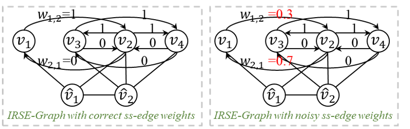
Although both of our classifiers are constructed using IRSE-Graph, their training procedures are slightly different. As for initial classifier, we directly train it on the initial IRSE-Graph without any pairwise ordering information (all ss-edge weights are set to 0.5). By contrast, we train iterative classifier on IRSE-Graph with partial pairwise orderings. To enable iterative classifier generalizable to any IRSE-Graph with partial predicted pairwise orderings, we first set all ss-edge weights to 1 or 0 according to their ground-truth pairwise orderings, and then train the classifier to correctly predict pariwise orderings for other pairs. Concretely, if $\boldsymbol{s}_{i}$ appears before $\boldsymbol{s}_{i^{\prime}}$, we set $w_{i,i^{\prime}}$$=$$1$ and $w_{i^{\prime},i}$$=$$0$, vice versa. For example, in the left part of Figure 3, the ground-truth sentence sequence is $s_{1}$,$s_{2}$,$s_{3}$,$s_{4}$, and thus we assign the ss-edge weights of linked sentence node pairs $(v_{1},v_{2})$, $(v_{3},v_{2})$, $(v_{3},v_{4})$, $(v_{2},v_{4})$ as follows: $w_{1,2}$$=$$1$, $w_{2,3}$$=$$1$, $w_{2,4}$$=$$1$, $w_{3,4}$$=$$1$, and $w_{2,1}$$=$$0$, $w_{3,2}$$=$$0$, $w_{4,2}$$=$$0$, $w_{4,3}$$=$$0$.

Moreover, to enhance the robustness of the iterative classifier, we randomly select a certain ratio $\eta$ of sentence pairs and assign their ss-edges with incorrect weights. Let us revisit Figure 3, for the randomly selected sentence node pair $(v_{1},v_{2})$, we assign ss-edges weights $w_{1,2}$ and $w_{2,1}$ with randomly generated noisy values 0.3 and 0.7 respectively. In this way, we expect that iterative classifier can conduct correct predictions even given incorrect previously-predicted pairwise orderings.

Finally, following the conventional SE-GRN Yin et al. 2019; Yin et al. 2021, we construct a graph-based sentence ordering model. Note that the above two classifiers and our sentence ordering model are all based on IRSE-Graph rather than the conventional SE-Graph, which makes the standard GRN unable to be applied directly. To deal with this issue, we slightly adapt GRN to utilize pairwise ordering information for graph encoding. Specifically, we adapt Equation 1 to incorporate ss-edge weights into the message aggregation of sentence-level nodes:

Here $\sigma$ denotes sigmoid function and $W_{g}$ is learnable parameter matrix. Equation 6 expresses that the sentence-level aggregation should consider not only the semantic representations of the two involved sentences, but also the relative ordering between them. In addition, other Equations are the same as those of conventional GRN, which have been described in Section §3.2.

Since pairwise ordering plays a crucial role in our proposed framework, we first compare the performance of different classifiers on various datasets. Table 2 shows the experimental results. Obviously, the utilization of iterative classifier further benefits the predictions of pairwise orderings.

Table 1 reports the overall experimental results of sentence ordering. When incorporating BERT and FHDecoder into IRSE-GRN, our model achieves SOTA performance on most of datasets. Besides, we arrive at the following conclusions:

First, IRSE-GRN significantly surpasses SE-GRN on all datasets (bootstrapping test, $p$$<$$0.01$), indicating that iteratively refining graph representations indeed benefit the ordering of input sentences.

Second, IRSE-GRN+FHDecoder exhibits better performance than IRSE-GRN and all non-BERT baselines, which are shown above the upper dotted line of Table 1, across datasets in different domains. Therefore, we confirm that our framework is orthogonal to the current approach exploiting pairwise ordering information for decoder.

Third, when constructing our model based on BERT, IRSE-GRN+BERT+FHDecoder also outperforms all BERT-based baselines, such as ConsGraph, BERSON, achieving SOTA performance. It can be known that our proposed framework is also effective when combining with pretrained language model.

Finally, we note that IRSE-GRN+BERT+FH-
Decoder gains relatively marginal improvement on SIND and ROCStory, and performs worse than BERSON in PMR on SIND. We speculate that there exist less ss-edges on these two datasets, resulting in that our proposed framework can not achieve its full potential. Specifically, average edge numbers of SIND and ROCStory are 2.85 and 5.66 respectively, far fewer than 16.60, 10.86 and 16.73 on NIPS Abstract, ANN Abstract and arXiv Abstract.

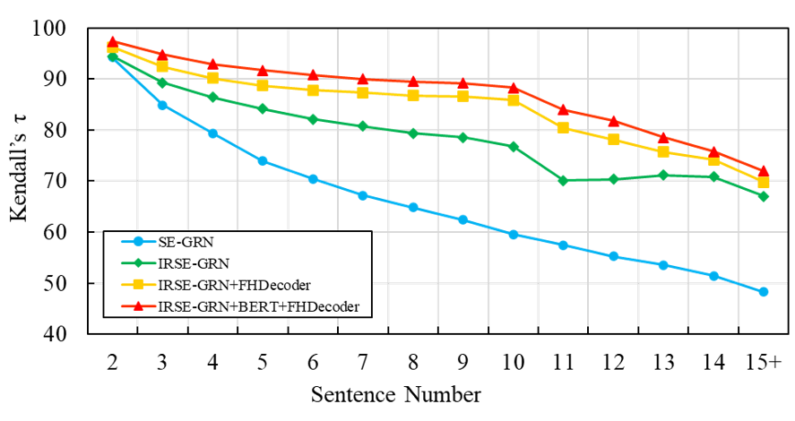
Besides, since it is a challenge to order longer paragraphs, we investigate the Kendall’s $\tau$ of our models and SE-GRN with respect to different sentence numbers, as shown in Figure 4. Overall, all models degrade with the increase of sentence number. However, our model and its two enhanced versions always exhibit better performance than SE-GRN.

As mentioned in previous studies Gong et al. 2016; Chen et al. 2016; Cui et al. 2018; Oh et al. 2019, the first and last sentences are very important in a paragraph. Following these studies, we compare models by conducting experiments to predict the first and last sentences.

As displayed in Table 3, IRSE-GRN surpasses all non-BERT baselines, and IRSE-GRN+BERT+ FHDecoder wins against BERTSON. These results are consistent with those reported in Table 1, further demonstrating the effectiveness of our model.

We conduct several experiments to investigate the impacts of our proposed components on ROCstory dataset and arXiv dataset which are the two largest datasets. All results are provided in Table 4, where we draw the following conclusions:

First, using only iterative classifier, IRSE-GRN(w/o initial classifier) performs worse than IRSE-GRN. This result proves that iterative classifier fails to predict well from scratch and the pairwise ordering predicted by initial classifier is beneficial to construct a well-formed graph representation for iterative classifier.

Second, when the iteration number k is set as 1, the performance of IRSE-GRN decreases. Moreover, if we remove iterative classifier, the performance of IRSE-GRN becomes even worse. Therefore, we confirm that the iterative predictions of pairwise ordering indeed benefit the learning of graph representations.

Finally, the result in the last line indicates that removing noisy weights leads to a significant performance drop. It suggests that the utilization of noisy weights is useful for the training of iterative classifier, which makes our model more robust.

Following previous studies Barzilay and Lapata 2005; Nayeem and Chali 2017, we further inspect the validity of our proposed framework via multi-document summarization. Concretely, we train different neural sentence ordering models on a large-scale summarization corpus Fabbri et al. 2019, and then individually use them to reorder the small-scale summarization data of DUC2004 (Task2). Finally, we use coherence probability proposed by Nayeem and Chali 2017 to evaluate the coherence of summaries. In this group of experiments, we conduct experiments using different weights: 0.5 and 0.8, as implemented in Nayeem and Chali 2017 and Yin et al. 2020 respectively.

The results are reported in Table 5. We can observe that the summaries reordered by IRSE-GRN and its variants achieve higher coherence probabilities than baseline, verifying the effectiveness of our proposed framework in the downstream task.

To provide more experimental results, we summarize the runtime on the validation sets and the numbers of parameters for our enhanced models and baseline SE-GRN in Table 6.

References

- Agrawal et al. (2016) Harsh Agrawal, Arjun Chandrasekaran, Dhruv Batra, Devi Parikh, and Mohit Bansal. 2016. Sort story: Sorting jumbled images and captions into stories. In EMNLP, pages 925–931.
- Barzilay et al. (2002) Regina Barzilay, Noemie Elhadad, and Kathleen R. McKeown. 2002. Inferring strategies for sentence ordering in multidocument news summarization. Journal of Artificial Intelligence Research, 17:35–55.
- Barzilay and Lapata (2005) Regina Barzilay and Mirella Lapata. 2005. Modeling local coherence: An entity-based approach. In ACL, pages 141–148.
- Barzilay and Lapata (2008) Regina Barzilay and Mirella Lapata. 2008. Modeling local coherence: An entity-based approach. Computational Linguistics, 34(1):1–34.
- Barzilay and Lee (2004) Regina Barzilay and Lillian Lee. 2004. Catching the drift: Probabilistic content models, with applications to generation and summarization. In NAACL, pages 113–120.
- Chen et al. (2016) Xinchi Chen, Xipeng Qiu, and Xuanjing Huang. 2016. Neural sentence ordering. arXiv:1607.06952.
- Chowdhury et al. (2021) Somnath Basu Roy Chowdhury, Faeze Brahman, and Snigdha Chaturvedi. 2021. Reformulating sentence ordering as conditional text generation. arXiv:2104.07064.
- Cui et al. (2018) Baiyun Cui, Yingming Li, Ming Chen, and Zhongfei Zhang. 2018. Deep attentive sentence ordering network. In EMNLP, pages 4340–4349.
- Cui et al. (2020) Baiyun Cui, Yingming Li, and Zhongfei Zhang. 2020. Bert-enhanced relational sentence ordering network. In EMNLP, pages 6310–6320.
- Deng et al. (2020) Chaorui Deng, Ning Ding, Mingkui Tan, and Qi Wu. 2020. Length-controllable image captioning. In ECCV, pages 712–729.
- Devlin et al. (2019) J. Devlin, Ming-Wei Chang, Kenton Lee, and Kristina Toutanova. 2019. Bert: Pre-training of deep bidirectional transformers for language understanding. In NAACL-HLT, pages 4171–4186.
- Elsner and Charniak (2011) Micha Elsner and Eugene Charniak. 2011. Extending the entity grid with entity-specific features. In ACL, pages 125–129.
- Fabbri et al. (2019) Alexander R. Fabbri, Irene Li, Tianwei She, Suyi Li, and Dragomir R. Radev. 2019. Multi-news: A large-scale multi-document summarization dataset and abstractive hierarchical model. In ACL, pages 1074–1084.
- Ghazvininejad et al. (2019) Marjan Ghazvininejad, Omer Levy, Yinhan Liu, and Luke Zettlemoyer. 2019. Mask-predict: Parallel decoding of conditional masked language models. In EMNLP-IJCNLP, pages 6111–6120.
- Gong et al. (2016) Jingjing Gong, Xinchi Chen, Xipeng Qiu, and Xuanjing Huang. 2016. End-to-end neural sentence ordering using pointer network. arXiv:1611.04953.
- Gu et al. (2018) Jiatao Gu, James Bradbury, Caiming Xiong, Victor O. K. Li, and Richard Socher. 2018. Non-autoregressive neural machine translation. In ICLR.
- Gui et al. (2020) Tao Gui, Jiacheng Ye, Qi Zhang, Zhengyan Li, Zichu Fei, Yeyun Gong, and Xuanjing Huang. 2020. Uncertainty-aware label refinement for sequence labeling. In EMNLP, pages 2316–2326.
- Guinaudeau and Strube (2013) Camille Guinaudeau and Michael Strube. 2013. Graph-based local coherence modeling. In ACL, pages 93–103.
- Holtzman et al. (2018) Ari Holtzman, Jan Buys, Maxwell Forbes, Antoine Bosselut, David Golub, and Yejin Choi. 2018. Learning to write with cooperative discriminators. In ACL, pages 1638–1649.
- Huang et al. (2016) Ting-Hao Huang, Francis Ferraro, Nasrin Mostafazadeh, Ishan Misra, Aishwarya Agrawal, Jacob Devlin, Ross Girshick, Xiaodong He, Pushmeet Kohli, Dhruv Batra, C. Lawrence Zitnick, Devi Parikh, Lucy Vanderwende, Michel Galley, and Margaret Mitchell. 2016. Visual storytelling. In NAACL, pages 1233–1239.
- Konstas and Lapata (2012) Ioannis Konstas and Mirella Lapata. 2012. Unsupervised concept-to-text generation with hypergraphs. In NAACL, pages 752–761.
- Kumar et al. (2020) Pawan Kumar, Dhanajit Brahma, Harish Karnick, and Piyush Rai. 2020. Deep attentive ranking networks for learning to order sentences. In AAAI, pages 8115–8122.
- Lapata (2003) Mirella Lapata. 2003. Probabilistic text structuring: Experiments with sentence ordering. In ACL, pages 545–552.
- Lewis et al. (2020) Mike Lewis, Yinhan Liu, Naman Goyal, Marjan Ghazvininejad, Abdelrahman Mohamed, Omer Levy, Veselin Stoyanov, and Luke Zettlemoyer. 2020. BART: denoising sequence-to-sequence pre-training for natural language generation, translation, and comprehension. In ACL, pages 7871–7880.
- Li and Jurafsky (2017) Jiwei Li and Dan Jurafsky. 2017. Neural net models of open-domain discourse coherence. In EMNLP, pages 198–209.
- Logeswaran et al. (2018) Lajanugen Logeswaran, Honglak Lee, and Dragomir R. Radev. 2018. Sentence ordering and coherence modeling using recurrent neural networks. In AAAI, pages 5285–5292.
- Mohiuddin et al. (2018) Muhammad Tasnim Mohiuddin, Shafiq R. Joty, and Dat Tien Nguyen. 2018. Coherence modeling of asynchronous conversations: A neural entity grid approach. In ACL, pages 558–568.
- Moon et al. (2019) Han Cheol Moon, Tasnim Mohiuddin, Shafiq R. Joty, and Xu Chi. 2019. A unified neural coherence model. In EMNLP-IJCNLP, pages 2262–2272.
- Mostafazadeh et al. (2016) Nasrin Mostafazadeh, Nathanael Chambers, Xiaodong He, Devi Parikh, Dhruv Batra, Lucy Vanderwende, Pushmeet Kohli, and James Allen. 2016. A corpus and cloze evaluation for deeper understanding of commonsense stories. In NAACL, pages 839–849.
- Nallapati et al. (2012) Ramesh Nallapati, Feifei Zhai, and Bowen Zhou. 2012. Summarunner: A recurrent neural network based sequence model for extractive summarization of documents. In AAAI, pages 3075–3081.
- Nayeem and Chali (2017) Mir Tafseer Nayeem and Yllias Chali. 2017. Extract with order for coherent multi-document summarization. In ACL TextGraphs Workshop, pages 51–56.
- Nguyen and Joty (2017) Dat Tien Nguyen and Shafiq Rayhan Joty. 2017. A neural local coherence model. In ACL, pages 1320–1330.
- Oh et al. (2019) Byungkook Oh, Seungmin Seo, Cheolheon Shin, Eunju Jo, and Kyong-Ho Lee. 2019. Topic-guided coherence modeling for sentence ordering by preserving global and local information. In EMNLP-IJCNLP, pages 2273–2283.
- Prabhumoye et al. (2020) Shrimai Prabhumoye, Ruslan Salakhutdinov, and Alan W. Black. 2020. Topological sort for sentence ordering. In ACL, pages 2783–2792.
- Radev et al. (2016) Dragomir R. Radev, Mark Thomas Joseph, Bryan R. Gibson, and Pradeep Muthukrishnan. 2016. A bibliometric and network analysis of the field of computational linguistics. Journal of the Association for Information Science and Technology, 67(3):683–706.
- Song et al. (2019) Linfeng Song, Daniel Gildea, Yue Zhang, Zhiguo Wang, and Jinsong Su. 2019. Semantic neural machine translation using AMR. Transactions of the Association for Computational Linguistics, 7:19–31.
- Song et al. (2020) Linfeng Song, Ante Wang, Jinsong Su, Yue Zhang, Kun Xu, Yubin Ge, and Dong Yu. 2020. Structural information preserving for graph-to-text generation. In ACL, pages 7987–7998.
- Song et al. (2018) Linfeng Song, Zhiguo Wang, Mo Yu, Yue Zhang, Radu Florian, and Daniel Gildea. 2018. Exploring graph-structured passage representation for multi-hop reading comprehension with graph neural networks. arXiv:1809.02040.
- Vinyals et al. (2015a) Oriol Vinyals, Meire Fortunato, and Navdeep Jaitly. 2015a. Pointer networks. In NIPS, page 3104–3112.
- Vinyals et al. (2015b) Oriol Vinyals, Meire Fortunato, and Navdeep Jaitly. 2015b. Pointer networks. In NIPS, pages 2692–2700.
- Wang and Wan (2019) Tianming Wang and Xiaojun Wan. 2019. Hierarchical attention networks for sentence ordering. In AAAI, pages 7184–7191.
- Xue et al. (2019) Mengge Xue, Weiming Cai, Jinsong Su, Linfeng Song, Yubin Ge, Yubao Liu, and Bin Wang. 2019. Neural collective entity linking based on recurrent random walk network learning. In IJCAI, pages 5327–5333.
- Yin et al. (2021) Yongjing Yin, Shaopeng Lai, Linfeng Song, Chulun Zhou, Xianpei Han, Junfeng Yao, and Jinsong Su. 2021. An external knowledge enhanced graph-based neural network for sentence ordering. Journal of Artificial Intelligence Research, 70:545–566.
- Yin et al. (2020) Yongjing Yin, Fandong Meng, Jinsong Su, Yubin Ge, Linfeng Song, Jie Zhou, and Jiebo Luo. 2020. Enhancing pointer network for sentence ordering with pairwise ordering predictions. In AAAI, pages 9482–9489.
- Yin et al. (2019) Yongjing Yin, Linfeng Song, Jinsong Su, Jiali Zeng, Chulun Zhou, and Jiebo Luo. 2019. Graph-based neural sentence ordering. In IJCAI, pages 5387–5393.
- Zeiler (2012) Matthew D. Zeiler. 2012. ADADELTA: an adaptive learning rate method. arXiv:1212.5701.
- Zhang et al. (2018) Yue Zhang, Qi Liu, and Linfeng Song. 2018. Sentence-state lstm for text representation. In ACL, pages 317–327.
- Zhu et al. (2021) Yutao Zhu, Kun Zhou, Jian-Yun Nie, Shengchao Liu, and Zhicheng Dou. 2021. Neural sentence ordering based on constraint graphs. In AAAI, pages 14656–14664.