Generating MCMC proposals by randomly rotating the regular simplexJournal: Journal of Multivariate Analysis
Abstract
We present the simplicial sampler, a class of parallel MCMC methods that generate and choose from multiple proposals at each iteration. The algorithm’s multiproposal randomly rotates a simplex connected to the current Markov chain state in a way that inherently preserves symmetry between proposals. As a result, the simplicial sampler leads to a simplified acceptance step: it simply chooses from among the simplex nodes with probability proportional to their target density values. We also investigate a multivariate Gaussian-based symmetric multiproposal mechanism and prove that it also enjoys the same simplified acceptance step. This insight leads to significant theoretical and practical speedups. While both algorithms enjoy natural parallelizability, we show that conventional implementations are sufficient to confer efficiency gains across an array of dimensions and a number of target distributions.
Keywords:
Haar measure , Markov chain Monte Carlo , Orthogonal group , Parallel MCMC.2020 MSC
Primary 65C05 , Secondary 65C601 Introduction
Generating random samples from probability distributions is a crucial task in many of the quantitative sciences. Markov chain Monte Carlo (MCMC) algorithms sample from target distributions by constructing Markov chains that maintain their targets as equilibrium distributions. The classic Metropolis-Hastings (MH) algorithm [21, 13] builds such a Markov chain by iteratively generating a single proposal state conditioned on the current state and randomly accepting or rejecting that proposal based on a ratio involving the target and proposal densities evaluated at the current and proposed states. The majority of MCMC techniques share this general structure, randomly proposing and accepting a single proposal at each iteration, but some relatively recent methods make use of multiple proposals (or, multiproposals) at each step with the goals of, e.g., reducing autocorrelation between Markov chain states or making better use of parallel computing resources.
Liu et al. 2000 develops the first such multiproposal technique, the multiple-try Metropolis algorithm (MTM). Each iteration of MTM starts by proposing multiple states , from a proposal distribution and choosing a candidate from among them with probability proportional to their respective target density values . After this, the MTM algorithm generates an additional states from the distribution . In the case that is symmetric, the MTM algorithm then accepts with probability
| (1) |
Whereas MTM is the most widely used multiproposal MCMC algorithm, it has certain drawbacks. First, to use proposals, one must generate states and evaluate the target density times. Second, after randomly selecting a potentially good candidate state , one might nonetheless reject it based on the target density values of the other proposed states within the Metropolis step that uses (1). Third, Yang and Liu 2021 rigorously prove superior mixing of MH over MTM albeit in the simplified setting of independence proposals. Perhaps most importantly, Tjelmeland 2004 shows that MTM’s additional Metropolis step and its extra noise are simply not necessary.
Next, Tjelmeland 2004 and Frenkel 2004 develop multiproposal MCMC algorithms that do not require the same binary accept-reject step as MTM. Tjelmeland 2004 posits a collection of random variables and a probability distribution with density that describes the probability of proposing the entire set given . Tjelmeland 2004 augments the state space with a random variable indicating as the current state of the Markov chain and iterates between generating proposals conditioned on the current state and randomly selecting a new value for with probabilities
| (2) |
In addition to these probabilities, Tjelmeland 2004 advances two further transition strategies and two structured proposal strategies, which we discuss below. Finally, he proposes building estimators using a weighted average with weights equal to the probabilities (2) and proves that this estimator is consistent assuming the chain converges to equilibrium. Frenkel 2004 also uses the probabilities (2) as weights to build the same estimator but in the context of statistical physics. Frenkel 2004 provides an informal physics argument for the correctness of his approach, stating that it fails to maintain detailed balance but does maintain ‘superdetailed’ balance. More recently, Calderhead 2014 adds an additional subroutine to the algorithm of Tjelmeland 2004 so that, at each MCMC iteration, one simulates a random walk on the finite state space composed of the states using transition probabilities closely related to (2). Ultimately, however, Yang et al. 2018 and Schwedes and Calderhead 2021 show that the weighted estimators of Tjelmeland 2004 and Frenkel 2004 constitute Rao-Blackwellizations over the index variable within the framework of Calderhead 2014 and thus enjoy reduced variance.
Despite theoretical results favoring the use of weighted estimators that feature all proposals at each step, there are practical downsides to this approach. Here, one must: either (1) save a massive tensor to memory, where is the total number of MCMC iterations; or (2) know what the estimand of interest is beforehand and maintain a running average of each MCMC iteration’s contribution to the weighted estimator. Importantly, Schwedes and Calderhead 2021 empirically demonstrate that the non-Rao-Blackwellized estimators of Calderhead 2014 can perform poorly when a small number of jumps occur between the states of the proposal set. On the one hand, this result is disconcerting because their experimental baseline of jumps for proposals performs much worse than jumps for the same number of proposals. Time spent iterating between proposed states is time not spent exploring the target distribution. On the other hand, these empirical results rely on a specific multiproposal scheme in which
| (3) |
and do not necessarily extend to other multiproposal strategies.
With this in mind, we consider it worthwhile to further develop structured multiproposal methods that maintain scalability while not requiring many jumps within the proposal set. As mentioned above, Tjelmeland 2004 proposes two strategies. Proposal alternative 1, or ‘P1’ , first generates a Gaussian random variable centered at the current state and next generates proposals centered at :
| (4) |
Here, the two -dimensional covariance matrices take the same form so that all share the same expected distance from the center . In some ways, the recent work of Luo and Tjelmeland 2019 builds on this proposal strategy. They extend this multiproposal’s simple star-shaped structure, where is the center and are the flairs, to general acyclic graphs and tailor their proposals to models with certain discrete structures. Unlike his first proposal alternative, Tjelmeland 2004’s Proposal alternative 2, or ‘P2’, only applies to the scenario when and constructs proposal sets that are equidistant from a center and ‘maximally spread’. Setting to equal , the current state of the Markov chain, this scheme satisfies the following relations:
| (5) | |||
In words, one first generates two independent random variables that are each uniformly distributed on the sphere and forces them to be orthogonal to each other. Next, one generates the normally distributed and obtains followed by and . Straightforward calculations show that the proposals , and are indeed the same distance from the center . Similar calculations show that the proposals , and are all equidistant from each other and together constitute an equilateral triangle with random edge lengths.
Tjelmeland 2004 does not specify how one might extend his second proposal alternative to accommodate multiproposals when . In the following, we accomplish this multivariate generalization by first noting that the equilateral triangle is a regular 2-simplex. Generally, a -dimensional space can hold as a many as points that are pairwise equidistant. If , the points that satisfy
identify a regular polytope called a -simplex. Fig. 1 shows the regular simplices that fit in 3-dimensional space. Fig. 2 shows Petrie polygon projections [7] that are helpful for visualizing higher dimensional regular simplices. While we use the regular simplex as our starting point, the multistep nature of (5) makes it unclear how one might actually generate proposals when , an endeavor that doubtless involves more random variables with more complicated relationships. To preserve simplicity in this multivariate setting, in Section 3 we generate proposals using a matrix distribution over the orthogonal group , which consists of matrices satisfying . Because is a compact topological group, it admits a unique normalized, left-invariant measure called the Haar measure [8]. In symbols,
for and a Borel set on . The Haar measure on is not only useful for constructing simple multivariate proposals: its uniformity helps maintain a simplified acceptance step as well (Theorem 2).
Bearing in mind the poor performance of simple multiproposal strategies when the number of jumps between proposals is small [26], we are motivated to develop structured multiproposal strategies that do not require Rao-Blackwellization, or many inter-proposal jumps, and thus spend more time exploring the entire target distribution. We therefore develop a multivariate multiproposal framework that maintains the principles of Tjelmeland 2004’s second proposal strategy while also achieving greater simplicity. In the following, we develop the simplicial sampler and its extensions, prove algorithmic correctness and demonstrate usefulness of our approach on a range of target distributions. We start by deriving sufficient conditions for simplifying the acceptance probabilities (2).
2 Simplified acceptance probabilities
We wish to sample from the target distribution with density for . Given the current Markov chain state , we use the following steps to advance the Markov chain.
- 1.
Propose states according to the distribution ;
- 2.
Calculate densities for ;
- 3.
Randomly select a single state from the set according to the simplified selection probabilities
(6) - 4.
Set .
This transition rule uses a modified acceptance probability (2) that does not include the proposal density terms. As such, it rarely leaves the target distribution invariant. We require a further sufficient condition to guarantee that is a stationary distribution for our Markov chain.
Proposition 1 (Tjelmeland 2004).
The Markov chain with the above transition rule maintains detailed balance with respect to the target distribution if satisfies
| (7) |
and so is a stationary distribution of the chain.
Proof.
Let be the transition kernel associated with the transition from an arbitrary state according to the above steps 1-4. Then
For any two states , , the following holds:
where we use assumption (7) in the third line. ∎
Although the proof of Proposition 1 is new, the result itself is a special case of a result from Tjelmeland 2004, who argues that his method constitutes a Gibbs sampler that leaves the joint and marginal distributions of invariant. Proposition 1 underlines what one may readily gather from the acceptance probabilities (2). Namely, it may sometimes prove useful to design multiproposals that maintain criterion (7) insofar as such proposals obviate the need for computing proposal densities. In the following, we show that the Gaussian centered multiproposal (4) provides just such a multiproposal mechanism. Under this scheme, consider the -vector obtained by removing the state , or the th column, from the proposal set and applying the vectorization operator. Integrating over all possible gives the conditional distribution of given :
If one does not adapt the proposal covariance , then one may precompute the covariance matrix inverse in time and store it using memory. In high-dimensional settings where such storage is not possible, one may store only the inverse covariance and fill the inverse covariance at each step with complexity using the formula . Once one has this inverse, the inner product term in each
requires floating point operations. The upshot is an cost to compute all proposal densities . But if one adapts following Haario et al. 2001, then this acceptance mechanism requires: an matrix inversion for the updated at each step; an Kronecker product to construct the covariance matrix; and the floating point operations to compute the proposal densities . Thankfully, it turns out, none of these computations are necessary.
Lemma 1.
Proof.
Let denote the generic probability density function evaluated at the right and conditioned on the left, and let an analogous multivariate Gaussian density with dependence on the covariance suppressed. For two arbitrary indices ,
In the third line, we use the Gaussianity and conditional independence structure of the multiproposal. In the fourth line, we use the symmetry of the Gaussian density function. ∎
This simple result fills in a gap in Tjelmeland 2004: namely, it relates the symmetry in a proposal strategy to a simplified acceptance mechanism (6). Moreover, subsequent work [11] builds on this result by examining cases in which structured proposals lead to simplified acceptance probabilities. In the following, we develop a multivariate extension of the multiproposal (5) and show that it also satisfies symmetry relation (7) and thus also qualifies for the simplified acceptance mechanism (6).
3 Simplicial sampling
We develop a proposal mechanism and a few variations that satisfy symmetry relation (7) and help our basic algorithm preserve reversibility with respect to the target . This method uses certain mathematical objects introduced in Section 1: namely, the regular -simplex, the orthogonal group and the uniform Haar measure over the orthogonal group . Start with a regular simplex identified by a set of fixed vertices that satisfies . Equating the number of new proposals with the state space dimension , the simplicial sampler generates and chooses from proposals as follows.
- 1.
Sample .
- 2.
Rotate and translate the simplicial vertices .
- 3.
Draw a single sample from with probability proportional to .
- 4.
Set .
In short, the simplicial sampler advances its Markov chain by randomly rotating a set of equidistant vertices about the current state (Fig. 3) and randomly selecting the next state from among all vertices of the resulting simplex.
A modified simplicial sampler that only generates a single proposal reduces to Barker’s acceptance criterion [3]
with a symmetric proposal distribution. Just as Barker’s criterion is suboptimal with respect to the Peskun ordering [23], our criterion is also suboptimal. With this in mind, Tjelmeland 2004 provides an algorithm that manipulates the acceptance probabilities (2), of which our simplified acceptance probabilities are a special case.
Importantly, the random rotation step satisfies symmetry relation (7).
Lemma 2.
Proof.
Start by translating coordinates so that . We want to show that for an arbitrary . We focus on the case , since the alternative case is trivial. Since the Haar measure is uniform on , we only need to show the existence of a rotation that maps
The key is recognizing that the unique reflection that exchanges and leaves all other vertices unchanged because they are equidistant from and and inhabit the hyperplane that splits them evenly. In symbols, for . Thus
and
It follows that is the desired rotation matrix .
∎
Fig. 4 provides a stylized visualization of this argument in the setting when represents a 60∘ rotation clockwise about . Taken together, Lemma 2 and Proposition 1 assert that the simplicial sampler maintains detailed balance with respect to the target distribution.
Theorem 1.
If the simplicial sampler’s multiproposal is -irreducible and absolutely continuous with respect to , then is the unique stationary and limiting distribution of the Markov chain, and the strong law of large numbers holds.
Proof.
The result is a simple combination of the sampler’s reversibility with respect to and the aperiodicity that arises from its self-loop, i.e., the ability to set to [28]. ∎
While -irreducibility is a major hypothesis of Theorem 1, we do not formally prove that the simplicial sampler exhibits generally irreducible behavior. That said, there are two intuitive reasons for thinking that the sampler produces generally irreducible Markov chains. First, the simplicial sampler can return to an arbitrarily small ball around a given state within just two steps with positive probability: the first iteration accepts a state away from the current state, and the second iteration accepts a state in the neighborhood of the preceding state. Second, the simplicial sampler can amble arbitrarily far away from a given state in the manner that a distracted geometry student can walk a compass clear off their desk. The need for a formally justified sampler leads us to randomly scale the proposal simplex in Section 3.1.1.
3.1 Variations
3.1.1 Gaussian simplicial sampling
If we scale the simplex edge lengths by the square root of a chi-square random variable, the proposals will have multivariate Gaussian marginal distributions. The orthogonal group acts transitively on the sphere , i.e., it takes any point on to any other [17]. For this reason, left multiplying a single point on by a Haar distributed rotation matrix is one method for drawing a sample from the sphere’s uniform distribution. On the other hand, it is a well known fact that one may obtain a standard -dimensional Gaussian vector by uniformly sampling a single point on the sphere and scaling that point by the square root of an independently sampled random variable with degrees of freedom. Randomly scaling the simplicial edge length in a similar manner provides the following variation that we call the Gaussian simplicial sampler.
- 1.
Independently sample and .
- 2.
Rotate, scale and translate the vertices .
- 3.
Draw a single sample from with probability proportional to .
- 4.
Set .
By the above discussion, each of the proposals for has a Gaussian marginal distribution with mean and covariance matrix , where is still the simplicial edge length. Because of its random scaling, a stronger result than Theorem 1 applies to the Gaussian simplicial sampler.
Corollary 1.
Any distribution with support is the unique stationary and limiting distribution of the Gaussian simplicial sampler that targets it, and the strong law of large numbers holds.
Proof.
All that needs to be established is -irreducibility and absolute continuity. The latter condition is accomplished by hypothesis. The former condition is accomplished by the sufficient condition [28] that
This condition is itself accomplished by the unbounded nature of the multiproposal’s scaling. All edges are scaled by the same random variable, and the symmetry of the proposal simplex is therefore maintained. Because the random scaling is independent of the random rotation, the conditions within the proof of Lemma 2 remain exactly the same. ∎
In Section 5, we show that its random scaling gives the Gaussian simplicial sampler improved performance for a multimodal target distribution.
3.1.2 Preconditioned simplicial sampling
For , a and real-valued matrix, the preconditioned simplicial sampler takes the following steps.
- 1.
Sample .
- 2.
Rotate, precondition and translate the vertices .
- 3.
Draw a single sample from with probability proportional to .
- 4.
Set .
The matrix is itself a rotation in the Euclidean space equipped with inner product (Fig. 5).
Corollary 2.
The guarantees of Theorem 1 apply to the preconditioned simplicial sampler as well.
Proof.
Corollaries 1 and 2 combine to guarantee a unique stationary distribution and strong law of large numbers for a preconditioned Gaussian simplicial sampler, and we explore this algorithm in Section 5.
3.1.3 Adaptive simplicial sampling
As has been established for other MCMC algorithms, it is often useful to adapt the simplicial sampler multiproposal. We employ two distinct methods of adaptation in Section 5. Both methods use the diminishing adaptation strategy [24], which sacrifices guarantees of a strong law of large numbers but maintains a weak law. The first adapts all simplex edge lengths while keeping them equal so as to achieve a desired ‘acceptance’ rate. Although the simplicial sampler does not use a classical accept-reject step, we can check whether state equals and call this an acceptance or rejection accordingly. The second adapts the preconditioning matrix following the proposal covariance adaptation outlined in Haario et al. 2001. In practice, we find it useful to combine these two adaptation schemes when implementing the preconditioned simplicial sampler.
3.1.4 Extra-dimensional simplicial sampling
The final variation for the simplicial sampler uses a number of proposals that is larger than the dimensionality of the target distribution, i.e., . Let be the wide matrix for which multiplication selects the first elements of any -vector. Letting each , , be a -dimensional vector, the extra-dimensional simplicial sampler works as follows.
- 1.
Sample .
- 2.
Rotate, precondition and translate the vertices .
- 3.
Draw a single sample from with probability proportional to .
- 4.
Set .
One may interpret the application of as a form of preconditioning with preconditioner . In Section 3.1.2, we argue that the guarantees of Lemma 2 apply to the preconditioned simplicial sampler because is a random rotation in Euclidean space with inner product . Following this analogy, we have
for the Moore-Penrose inverse [14]. Due to the degeneracy of , the resulting form is no longer an inner product, and we cannot assert that the extra-dimensional algorithm inherits the promises of Lemma 2. Nonetheless, limited empirical experiments do show the algorithm providing accurate results, and we find it helpful to visualize the sampler in Section 5.3.
4 Computational considerations
The real-world performance of an algorithm depends on its computational complexity, the language it is written in and the hardware it is implemented on. It also depends on how well one codes it up, e.g., efficient use of random access memory and parallelization when available. We separate these considerations into multiproposal and acceptance mechanisms, and the exact weight one assigns to the two steps will depend on the computational complexity of the target distribution.
4.1 Multiproposal mechanisms
4.1.1 The simplicial sampler multiproposal
The simplicial sampler requires the generation of a random rotation . The most common way to perform this step is to generate a matrix of standard normals and then perform the QR factorization. Once one has the orthogonal ‘Q’ matrix, one right multiplies it by a diagonal matrix consisting of the signs of the diagonal of the ‘R’ matrix, guaranteeing that the obtained matrix is the unique orthogonal matrix corresponding to the with positive diagonal elements. Thus, one obtains using the QR factorization. There are additional algorithms for sampling from the Haar distribution over that provide speedups while still maintaining cubic complexity [27, 2]. In particular, Stewart 1980 achieves a 50% speedup over the QR factorization based algorithm by iteratively pre-multiplying random Householder matrices of increasing dimensions. We are interested in the fact that, when one only requires the random rotation and not the matrix itself, Stewart 1980’s algorithm only requires floating point operations to randomly rotate a -vector. On the one hand, the simplicial sampler multiproposal still requires floating point operations because it must apply this random rotation to the -vectors that identify the regular simplex. On the other hand, one could apply this algorithm in an embarrassingly parallel manner to the non-zero -vectors that contribute to the regular simplex. Furthermore, the entirety of the algorithm relies on matrix-matrix multiplications and should be extremely fast and scalable on a modern GPU: Li et al. 2013 use a (now outdated) Tesla C1060 GPU to score 10,000-fold speedups over a single-core -algorithm implementation written in C++. Such a fast GPU implementation of Stewart 1980’s algorithm requires significant engineering that is a contribution in its own right, so we focus on conventional implementations in the following.
Finally, even for serial implementations, the language of implementation can eclipse theoretical computational complexity. We find that an R based implementation of Stewart 1980’s algorithm is much slower than the QR factorization based method implemented in the PRACMA [5] R package. The QR decomposition in R calls the Fortran library LAPACK to perform the numerical linear algebra for the QR decomposition, and its precompiled and memory efficient implementation outperform interpreted R.
4.1.2 Other multiproposals
If one precomputes , the multiproposals (3) and (4) are of complexity , with the majority of time spent multiplying the square-root covariance by a matrix of standard normals. If one adopts the preconditioning strategy of Haario et al. 2001, the complexity changes to accounting for a Cholesky decomposition. If one specifies , then the complexity drops to , and the new bottleneck becomes generation of i.i.d. standard normals.
Just as for the simplicial sampler’s random rotations, one may parallelize the matrix multiplications for these multiproposals. One may also parallelize the standard normal generations using the parallel pseudo random number generators of Salmon et al. 2011 that TensorFlow uses Abadi et al. 2016 to great success.
4.2 Acceptance mechanisms
The simplified acceptance mechanism (6) requires target density evaluations. These density evaluations are embarrassingly parallel, but there are some target distributions for which this kind of parallelization is not necessary. When one jointly infers a multivariate Gaussian random variable and its covariance matrix using Metropolis-within-Gibbs, one must invert the updated covariance every time one updates the Gaussian variable. Once one has inverted the covariance matrix, evaluating the multivariate Gaussian density over proposals is almost as fast as evaluating the density over a single proposal. That said, this intuition also applies to Metropolis-within-Gibbs with a simple random walk Metropolis update: having updated and inverted the covariance matrix, one may perform many Metropolis updates of the Gaussian random variable at relatively little additional cost. In general, however, careful parallelization should help accelerate the acceptance step for multiproposal methods in a way unavailable to single-proposal methods. For example, Holbrook 2021 uses a quantum computer to achieve quadratic speedups that reduce the number of target evaluations from to .
The simplified acceptance mechanism also avoids potentially costly computations of the proposal densities required for the general acceptance mechanism (2). For example, the i.i.d. multiproposal (3) requires an additional computational cost to obtain the terms
On the other hand, Lemma 1 shows that the centered Gaussian multiproposal (4) leads to a simplified acceptance mechanism that results in prodigious theoretical speedups thoroughly discussed in Section 3.
5 Results
In the following, we use (PC-)Simpl, (PC-)RWM and (PC-)MTM to indicate the (preconditioned) simplicial sampler, random walk and multiple-try Metropolis algorithms, respectively. Although PC-RWM is better known as the adaptive Metropolis algorithm of Haario et al. 2001, we use this notation to clarify comparisons. ESS and ESSs denote effective sample size and effective sample size per second, respectively. All experiments use the R language [16] and the R package pracma [5] to produce random rotations, which itself uses the QR decomposition of a matrix with Gaussian entries (Section 4.1.1). All MTM simulations use proposals for comparison. Finally, all results herein rely on a conventional single-core implementation.
5.1 Empirically optimal scaling
5.1.1 Acceptance rates and edge lengths
We first investigate Simpl and PC-Simple performance for Gaussian targets of varying dimensions (4 through 500) as a function of acceptance rate and simplex edge length. For each dimension, we employ 20 independent MCMC runs of 10,000 iterations targeting one of 20 acceptance rates uniformly spaced between 0.2 and 0.95 (Section 3.1.3). The ‘ill-conditioned’ Gaussian target has diagonal covariance with elements 1 through . The left two panels of Fig. 6 plot the acceptance rates or edge lengths that maximize minimum and mean ESS out of the 20 targeted. For both Simpl and PC-Simpl, optimal acceptance rates increase with dimensionality until flattening out at around 0.675. For Simpl, optimal edge lengths quickly flatten out at around 3. For PC-Simpl, optimal edge lengths grow with target dimension.
5.1.2 Number of proposals
In general, Simpl uses a simplex with nodes, the maximal number available in dimensions. The right panel of Fig. 6 shows ESS results when lower dimensional simplices (with fewer nodes) are used to generate fewer proposals (). In practice, one may implement such a variation by replacing the initial set of pre-rotated vectors with , again letting . Algorithmic details otherwise remain the same. We use 100 independent MCMC runs of 10,000 iterations each to generate minimum and mean ESS across target dimensions. Both measures improve with greater numbers of proposals. We do not compare ESSs because the additional cost of a simplex node arises from a mere matrix-vector multiplication, compared to the generation of a random rotation.
5.2 Performance comparisons
5.2.1 Accelerated centered Gaussian multiproposal
Fig. 7 compares the simplicial sampler performance to that of the centered Gaussian sampler (4) using and proposals. The ‘slow’ Gaussian centered multiproposal calculates all proposal probabilities , whereas the ‘fast’ sampler uses the simplified acceptance probabilities (6) following Lemma 1. Samplers target a standard spherical normal distribution and a 50% acceptance rate for 10,000 iterations. In terms of ESS, doubling the number of proposals appears to benefit the centered Gaussian sampler, especially in lower dimensions. The fast implementation of the centered Gaussian sampler already starts to outperform the slow implementations in lower dimensions, and this relative performance gain only increase with dimensions. Across all dimensions, the ESSs trajectory of the simplicial sampler remains firmly in between those of the fast and slow centered Gaussian samplers.
5.2.2 Gaussian targets
We compare vanilla algorithms on spherical targets of dimensions 4, 8, 16, 32, 64, 128, 256 and 512, all with identity for covariance matrix, and preconditioned algorithms on targets with ill-conditioned diagonal and full covariance matrices. Ill-conditioned matrices all have spectra ranging uniformly from 1 to . RWM and MTM both use optimal scaling of [10]. For the latter, this results in an asymptotic 30% acceptance rate as gets large [4]. Simpl adapts to empirically optimal acceptance rates of Fig. 6. Fig. 8 shows relative ESS and ESSs results from 10 independent MCMC runs of 10,000 iterations each per algorithm. Since ESS is a univariate measure, we report means and minima with respect to target dimensions.
5.2.3 Bimodal target
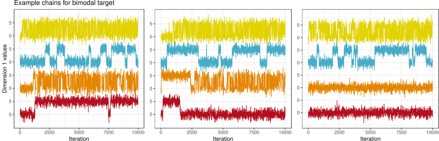
In general, Gaussian simplicial sampling (G-Simpl) (Section 3.1.1) and its preconditioned form (PCG-Simpl) perform slightly worse ( less ESS) than Simpl and PC-Simpl on unimodal targets, but G-Simpl and PCG-Simpl perform better on multimodal targets. We compare G-Simpl and PCG-Simpl to RWM and PC-RWM on mixture of Gaussian targets of dimensions 2, 3 and 4. Mixture probabilities are - and covariances are identity, but modal means are and . Thus, modes become farther apart with increasing dimension. Fig. 9 shows stacked traceplots and boxplots for the number of intermodal jumps recorded from 100 independent MCMC runs of 100,000 iterations each.
5.2.4 Gaussian process classification
| Algorithm | Mean ESS | Min ESS | Its to | ESS | ESS | ESS | ESS |
|---|---|---|---|---|---|---|---|
| Simpl | 1571.50 (15.6) | 256.27 (6.4) | 73.05 (1.8) | 671.39 (10.2) | 2463.76 (76.6) | 3703.05 (50.0) | 452.30 (6.7) |
| RWM | 436.34 (2.3) | 68.36 (2.3) | 276.60 (8.3) | 258.63 (5.7) | 1407.88 (61.8) | 1837.47 (31.3) | 134.91 (2.3) |
| MTM | 1195.22 (12.8) | 252.13 (7.3) | 1928.75 (20.5) | 676.75 (12.8) | 2332.81 (84.9) | 3490.12 (58.41) | 366.86 (6.3) |
| PC-Simpl | 1865.18 (14.4) | 1200.50 (20.4) | 76.39 (2.2) | 1312.98 (18.0) | 4583.21 (95.5) | 4222.10 (50.7) | 532.49 (6.5) |
| PC-RWM | 362.99 (4.5) | 205.16 (5.3) | 284.27 (10.5) | 418.99 (10.9) | 1381.00 (37.6) | 1654.35 (29.8) | 125.12 (3.0) |
| PC-MTM | 1256.07 (15.9) | 755.42 (16.4) | 1873.89 (21.1) | 951.97 (15.3) | 3840.86 (88.3) | 3736.27 (48.0) | 272.08 (6.3) |
| Mean ESSs | Min ESSs | Time to | ESSs | ESSs | ESSs | ESSs | |
| Simpl | 5.62 (0.06) | 0.92 (0.02) | 15.87 (0.98) | 2.40 (0.04) | 8.81 (0.28) | 13.24 (0.18) | 1.62 (0.02) |
| RWM | 2.50 (0.02) | 0.39 (0.01) | 145.41 (9.69) | 1.48 (0.03) | 8.09 (0.36) | 10.55 (0.19) | 0.77 (0.01) |
| MTM | 3.85 (0.04) | 0.81 (0.02) | 11674.88 (252.45) | 2.18 (0.04) | 7.52 (0.27) | 11.25 (0.19) | 1.18 (0.02) |
| PC-Simpl | 5.09 (0.13) | 3.30 (0.10) | 23.99 (1.46) | 3.58 (0.10) | 12.59 (0.43) | 11.53 (0.32) | 1.45 (0.04) |
| PC-RWM | 1.44 (0.04) | 0.81 (0.03) | 268.77 (39.96) | 1.65 (0.06) | 5.48 (0.22) | 6.54 (0.21) | 0.49 (0.02) |
| PC-MTM | 3.87 (0.05) | 2.33 (0.05) | 11540.43 (269.22) | 2.93 (0.05) | 11.85 (0.28) | 11.53 (0.15) | 0.84 (0.02) |
48 states use a winner-take-all rule when assigning electoral college votes during the U.S. presidential election. We use a Gaussian process (GP) with logit link [30] to regress binary outcomes (Trump or Clinton) over state center (latitude and longitude) and population data for the 2016 presidential election. For latent variables , the prior covariance of and is
where and are their respective predictor vectors. We infer latent variables using (PC-)Simple, (PC-)RWM and (PC-)MTM. We let Simpl algorithms target an acceptance rate of 0.5 following the results of Fig. 6, while we let RWM, MTM and PC-MTM target 0.234, 0.3 and 0.4. The former value is optimal for RWM [24].The last two values appear advantageous in preliminary tests. We infer other parameters using univariate slice samplers [22]. Table 1 shows results from 100 independent runs of 100,000 iterations each. We initialize all chains to misclassify all states and use a total misclassification of 10 as rough convergence threshold. While Simple and MTM require multiple target evaluations at each step, they only must compute the GP inverse covariance once for all such evaluations. These results only establish effectiveness of the simplicial sampler relative to a few basic samplers and do not establish superiority relative to all samplers. Gradient-based MCMC methods could likely outperform the simiplicial sampler, but we abstain from such comparisons in order to focus on ‘apples-to-apples’ comparisons among non-gradient methods.
5.3 Visualizing the extra-dimensional simplicial sampler
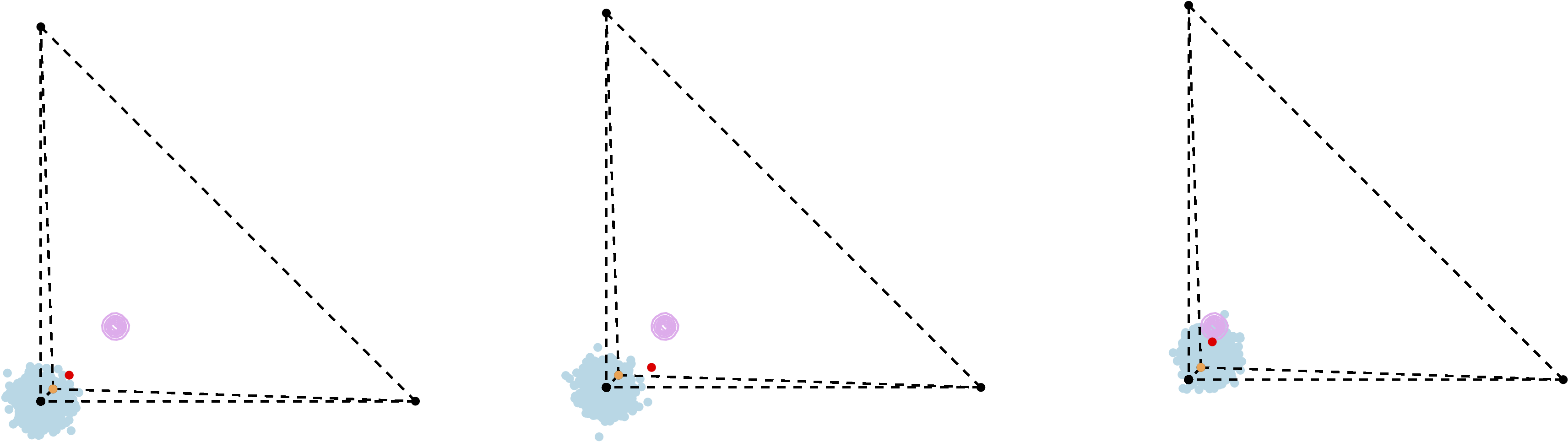
Because of the diminishing returns (Fig. 6, right) and computational cost associated with increasing the number of simplex vertices, the extra-dimensional simplicial sampler is not practical in the absence of advanced parallelization techniques. Moreover, the rotated vertices no longer maintain equal distances from each other in the low-dimensional space over which the target is defined. Fig. 10 shows three successive iterations of the extra-dimensional simplicial sampler with 1000 proposals targeting a 2D Gaussian distribution. The sampler successfully moves to the high-density region of the space in these three steps. We observe that rotating and projection the simplex vertices results in proposal point clouds that look plausibly Gaussian distributed, apparently lacking any geometric structure.
6 Discussion
We have developed the simplicial sampler, a multivariate extension of the multiproposal mechanism (5) from Tjelmeland 2004, and proven that this extension maintains detailed balance using simplified acceptance probabilities. We have shown that a variation on this algorithm, the Gaussian simplicial sampler, maintains a unique stationary distribution and an appropriate law of large numbers. Furthermore, we have proven that the centered Gaussian proposal mechanism (4) from Tjelmeland 2004 enables the same simplified acceptance probability that leads to significant speedups. We have thoroughly discussed the computational issues that one must consider when implementing these algorithms. Among others, these considerations include: theoretical computational complexity, hardware, programming language, efficient use of memory and parallelization. Finally, we have thoroughly compared performance of sequential implementations on a collection of target distributions. That said, we note that these algorithms are well suited for parallelization enabled by, e.g., a GPU or a quantum computer [15].
We are interested in two lines of further investigation. First, we have shown that two structurally distinct multiproposal mechanisms have symmetries that enable simplified acceptance probabilities. Are these the only such mechanisms or are there others? Can one combine these in ways that preserve the simplified acceptance probabilities? Finally, do analogues for these methods exist in discrete settings, e.g., for lattice models? Second, we are interested in the quality of convergence for the broader class of multiproposal MCMC algorithms. Based on simulations, it would not be surprising for geometric ergodicity to hold for these algorithms. Moreover, one might expect for mixing speeds to improve as the number of proposals increases.
Acknowledgments
This work was supported by NIH grant K25 AI153816 and NSF grant DMS 2152774. We thank Nathan Glatt-Holtz, Cecilia Mondaini and Justin Krometis for helpful discussions and advice.
Appendix A Empirical validation

Fig. 11 shows quantile-quantile (QQ) plots for the vanilla simplicial sampler for two different 3D Gaussian target distributions, one of which is spherical and the other of which has diagonal covariance with standard deviations 1, 2 and 3. The QQ plots demonstrate that the empirical quantiles of the simplicial sampler adhere closely to the quantiles of respective target distributions.
References
- Abadi et al. [2016] M. Abadi, A. Agarwal, P. Barham, E. Brevdo, Z. Chen, C. Citro, G. S. Corrado, A. Davis, J. Dean, M. Devin, et al., Tensorflow: Large-scale machine learning on heterogeneous distributed systems, arXiv preprint arXiv:1603.04467 (2016).
- Anderson et al. [1987] T. W. Anderson, I. Olkin, L. G. Underhill, Generation of random orthogonal matrices, SIAM Journal on Scientific and Statistical Computing 8 (1987) 625–629.
- Barker [1965] A. A. Barker, Monte carlo calculations of the radial distribution functions for a proton? electron plasma, Australian Journal of Physics 18 (1965) 119–134.
- Bédard et al. [2012] M. Bédard, R. Douc, E. Moulines, Scaling analysis of multiple-try mcmc methods, Stochastic Processes and their Applications 122 (2012) 758–786.
- Borchers [2021] H. W. Borchers, pracma: Practical Numerical Math Functions, 2021. R package version 2.3.3.
- Calderhead [2014] B. Calderhead, A general construction for parallelizing metropolis- hastings algorithms, Proceedings of the National Academy of Sciences 111 (2014) 17408–17413.
- Coxeter [1973] H. S. M. Coxeter, Regular Polytopes, Courier Corporation, New York, 1973.
- Folland [2016] G. B. Folland, A Course in Abstract Harmonic Analysis, volume 29, CRC press, Boca Raton, Florida, 2016.
- Frenkel [2004] D. Frenkel, Speed-up of monte carlo simulations by sampling of rejected states, Proceedings of the National Academy of Sciences 101 (2004) 17571–17575.
- Gelman et al. [1997] A. Gelman, W. R. Gilks, G. O. Roberts, Weak convergence and optimal scaling of random walk Metropolis algorithms, The Annals of Applied Probability 7 (1997) 110–120.
- Glatt-Holtz et al. [2022] N. E. Glatt-Holtz, A. J. Holbrook, J. A. Krometis, C. F. Mondaini, Parallel mcmc algorithms: Theoretical foundations, algorithm design, case studies, 2022.
- Haario et al. [2001] H. Haario, E. Saksman, J. Tamminen, An adaptive Metropolis algorithm, Bernoulli 7 (2001) 223–242.
- Hastings [1970] W. K. Hastings, Monte Carlo sampling methods using Markov chains and their applications, Biometrika 57 (1970) 97–109.
- Holbrook [2018] A. Holbrook, Differentiating the pseudo determinant, Linear Algebra and its Applications 548 (2018) 293–304.
- Holbrook [2021] A. J. Holbrook, A quantum parallel markov chain monte carlo, arXiv preprint arXiv:2112.00212 (2021).
- Ihaka and Gentleman [1996] R. Ihaka, R. Gentleman, R: a language for data analysis and graphics, Journal of Computational and Graphical Statistics 5 (1996) 299–314.
- Lee [2012] J. M. Lee, Quotient Manifolds, Springer New York, New York, NY, 2012, pp. 540–563.
- Li et al. [2013] J. Li, S. Ranka, S. Sahni, Gpu matrix multiplication, Multicore Computing: Algorithms, Architectures, and Applications 345 (2013).
- Liu et al. [2000] J. S. Liu, F. Liang, W. H. Wong, The multiple-try method and local optimization in metropolis sampling, Journal of the American Statistical Association 95 (2000) 121–134.
- Luo and Tjelmeland [2019] X. Luo, H. Tjelmeland, A multiple-try metropolis–hastings algorithm with tailored proposals, Computational Statistics 34 (2019) 1109–1133.
- Metropolis et al. [1953] N. Metropolis, A. W. Rosenbluth, M. N. Rosenbluth, A. H. Teller, E. Teller, Equation of state calculations by fast computing machines, The Journal of Chemical Physics 21 (1953) 1087–1092.
- Neal [2003] R. M. Neal, Slice sampling, The Annals of Statistics 31 (2003) 705 – 767.
- Peskun [1973] P. H. Peskun, Optimum monte-carlo sampling using markov chains, Biometrika 60 (1973) 607–612.
- Rosenthal [2011] J. S. Rosenthal, Optimal proposal distributions and adaptive mcmc, Handbook of Markov Chain Monte Carlo (2011) 119–138.
- Salmon et al. [2011] J. K. Salmon, M. A. Moraes, R. O. Dror, D. E. Shaw, Parallel random numbers: As easy as 1, 2, 3, in: Proceedings of 2011 International Conference for High Performance Computing, Networking, Storage and Analysis, SC ’11, Association for Computing Machinery, New York, NY, USA, 2011.
- Schwedes and Calderhead [2021] T. Schwedes, B. Calderhead, Rao-Blackwellised parallel MCMC, in: A. Banerjee, K. Fukumizu (Eds.), Proceedings of The 24th International Conference on Artificial Intelligence and Statistics, volume 130 of Proceedings of Machine Learning Research, PMLR, 2021, pp. 3448–3456.
- Stewart [1980] G. W. Stewart, The efficient generation of random orthogonal matrices with an application to condition estimators, SIAM Journal on Numerical Analysis 17 (1980) 403–409.
- Tierney [1994] L. Tierney, Markov chains for exploring posterior distributions, The Annals of Statistics 22 (1994) 1701–1728.
- Tjelmeland [2004] H. Tjelmeland, Using All Metropolis-Hastings Proposals to Estimate Mean Values (Norwegian University of Science and Technology, Trondheim, Norway), Technical Report, Tech Rep 4, 2004.
- Williams and Barber [1998] C. K. Williams, D. Barber, Bayesian classification with Gaussian processes, IEEE Transactions on Pattern Analysis and Machine Intelligence 20 (1998) 1342–1351.
- Yang et al. [2018] S. Yang, Y. Chen, E. Bernton, J. S. Liu, On parallelizable Markov chain Monte Carlo algorithms with waste-recycling, Statistics and Computing 28 (2018) 1073–1081.
- Yang and Liu [2021] X. Yang, J. S. Liu, Convergence rate of multiple-try metropolis independent sampler, arXiv preprint arXiv:2111.15084 (2021).