跳到论文正文
W Papers独立论文阅读器 arXiv:2110.06216 论文正文 计算阅读时间 · 0%
引用这篇论文根据当前论文元数据生成,正式投稿前建议核对。


License: arXiv.org perpetual non-exclusive license
arXiv:2110.06216v3 [cond-mat.str-el] 18 Apr 2022

Mechanism for particle fractionalization and universal edge physics
in quantum Hall fluids

A. Bochniak1,2, Z. Nussinov3, A. Seidel3, and G. Ortiz4, Email: ortizg@iu.edu Affiliation: 1 Institute of Theoretical Physics, Jagiellonian University, Łojasiewicza 11, 30-348 Kraków, Poland
2 Department of Mathematics, Indiana University, Bloomington, IN 47405, USA
3 Department of Physics, Washington University in St. Louis, MO 63160, USA
4 Department of Physics, Indiana University, Bloomington, IN 47405, USA
Abstract

Advancing a microscopic framework that rigorously unveils the underlying topological hallmarks of fractional quantum Hall (FQH) fluids is a prerequisite for making progress in the classification of strongly-coupled topological matter. Here we advance a second-quantization framework that helps reveal an exact fusion mechanism for particle fractionalization in FQH fluids, and uncover the fundamental structure behind the condensation of non-local operators characterizing topological order in the lowest-Landau-level (LLL). We show the first exact analytic computation of the quasielectron Berry connections leading to its fractional charge and exchange statistics, and perform Monte Carlo simulations that numerically confirm the fusion mechanism for quasiparticles. Thus, for instance, two quasiholes plus one electron of charge ee lead to an exact quasielectron of fractional charge e/3e/3, and exchange statistics 1/31/3, in a ν=1/3\nu=1/3 Laughlin fluid. We express, in a compact manner, the sequence of (both bosonic and fermionic) Laughlin second-quantized states highlighting the lack of local condensation. Furthermore, we present a rigorous constructive subspace bosonization dictionary for the bulk fluid and establish universal long-distance behavior of edge excitations by formulating a conjecture based on the DNA, or root state, of the FQH fluid.

Keywords: 
Topological Matter || Fractional Excitations || Universal Edge Physics ||

I Introduction

Fractional quantum Hall (FQH) fluids have long constituted the best known paradigm of strongly-correlated topological systems Jain 2007. Nonetheless, several fundamental issues remain unresolved. These include the exact mechanism leading to the quasiparticle (or fractional electron) excitations and viable universal signatures in edge transport that are rooted in the topological characteristics of the bulk FQH fluid. This state of affairs is partially due to a dearth of rigorous microscopic approaches capable of dealing with these highly entangled systems. A case in point is a first-principles computation of the quasielectron exchange statistics. In Bandyopadhyay et al. 2018, the Entangled Pauli Principle (EPP) was advanced as an organizing principle for FQH ground states. The EPP provides information about the pattern of entanglement of the complete subspace of zero-energy modes, i.e., ground states, of quantum Hall parent Hamiltonians for both Abelian and non-Abelian fluids. Those states are generated from the so-called “DNA” Bandyopadhyay et al. 2018, or root patterns Bernevig and Haldane 2008; Ortiz et al. 2013, which encode the elementary topological characteristics of the fluid.

In this work we advance second-quantization many-body techniques that allow for new fundamental insights into the nature of quasiparticle excitations of FQH liquids. In particular, we present an exact fractionalization procedure that allows for a very natural fusion mechanism of quasiparticle generation. We determine the quasihole and quasiparticle operators that explicitly flesh out Laughlin’s flux insertion/removal mechanism and provide the associated quasielectron wave function. The quasielectron that we find differs from Laughlin’s original proposal Laughlin 1983. We determine the Berry connection of this quasielectron wave function, considered as an Ehresmann connection on a principal fiber bundle, and as a result a natural fusion mechanism gets unfolded. This, in turn, leads to the exact determination of the quasielectron fractional charge. We perform Monte Carlo simulations to numerically confirm this fusion mechanism of fractionalization. In addition, we introduce an unequivocal diagnostic for characterizing and detecting the topological order of the FQH fluid in terms of a condensation of a non-local operator and present a constructive subspace bosonization (fermionization) dictionary for the bulk fluid that highlights the topological nature of the underlying theory. Our organizing EPP and the corresponding fluid’s DNA encode universal features of the bulk FQH state and its edge excitations. Here we formulate a conjecture that enables a demonstration of the universal long-distance behavior of edge excitations in weak confining potentials. This is based on the exact computation of the edge Green’s function over the DNA or root state of the topological fluid.

Although our main results are derived in a field-theoretical manner, we will reformulate some of our conclusions in a first quantization language, where states become wave functions. For clarity, we will occasionally use a mixed representation.

II States and Operator Algebra
in the LLL

The LLL is spanned by single-particle orbitals ϕr​(x,y)\phi_{r}(x,y) whose functional form depends on geometry Ortiz et al. 2013. We consider genus zero manifolds such as those of the disk and the cylinder. Lengths are measured in units of the magnetic length ℓ=ℏ​c|e|​B\ell=\sqrt{\frac{\hbar c}{|e|B}}, where BB is the magnetic field strength, ℏ\hbar the reduced Planck constant, cc the speed of light, and |e||e| the magnitude of the elementary charge. For ease of presentation, we will primarily focus on the disk geometry 11 1 One can always apply a similarity transformation to map to the cylinder Ortiz et al. 2013.. Then, ϕr​(z=x+𝗂​y)=zr/𝒩r\phi_{r}(z=x+{\sf i}y)=z^{r}/\mathcal{N}_{r}, 𝒩r=2​π​2r​r!\mathcal{N}_{r}=\sqrt{2\pi 2^{r}r!}, with r≥0r\geq 0 a non-negative integer labeling the angular momentum and z∈ℂz\in\mathbb{C} 22 2 Normalization is defined as ∫𝒟⁡[z]​(z∗)r​zr′=𝒩r2​δr,r′\int{\cal D}[z](z^{*})^{r}z^{r^{\prime}}={\cal N}_{r}^{2}\delta_{r,r^{\prime}} with 𝒟⁡[z]=d2​z​e−12​|z|2{\cal D}[z]=d^{2}z\,e^{-\frac{1}{2}|z|^{2}}, z∗=x−𝗂​yz^{*}=x-{\sf i}y, and magnetic unit length ℓ=1\ell=1.. NN-particle states (elements of the Hilbert space ℋLLL\mathcal{H}_{\mathrm{LLL}}) belong to either the totally symmetric (bosons) or anti-symmetric (fermions) representations of the permutation group SNS_{N}. Whenever results apply to either representation, we use second-quantized creation (annihilation) ar†a_{r}^{\dagger} (ara_{r}^{\;}) operators instead of the usual cr†c_{r}^{\dagger} (crc_{r}^{\;}), br†b_{r}^{\dagger} (brb_{r}^{\;}), for fermions and bosons, respectively. The field operator

Λ​(z)=∑r≥0ϕr​(z)​ar,\displaystyle\Lambda^{\;}(z)=\sum_{r\geq 0}\phi_{r}(z)a_{r}^{\;}, (1)

and its adjoint Λ†​(z)\Lambda^{\dagger}(z) satisfy canonical (anti-)commutation relations: [Λ​(z),Λ​(z′)]±=0[\Lambda^{\;}(z),\Lambda^{\;}(z^{\prime})]_{\pm}=0, [Λ​(z),Λ†​(z′)]±={z′|z}[\Lambda^{\;}(z),\Lambda^{\dagger}(z^{\prime})]_{\pm}=\{z^{\prime}|z\}, where {z′|z}=12​π​ez​z′⁣∗2\{z^{\prime}|z\}=\frac{1}{2\pi}e^{\frac{zz^{\prime\ast}}{2}} is a bilocal kernel satisfying ∫𝒟⁡[z]​Λ​(z)​{z|z′}=Λ⁡(z′)\int\mathcal{D}[z]\,\Lambda(z)\{z|z^{\prime}\}=\Lambda(z^{\prime}) Stone 1992. Many-particle states |ψ⟩∈ℋLLL|\psi\rangle\in\mathcal{H}_{\mathrm{LLL}} are characterized by the number of particles NN and the maximal occupied orbital rmaxr_{\mathrm{max}}, defining a filling factor ν=(N−1)/rmax\nu=(N-1)/r_{\mathrm{max}}. Given an antisymmetric holomorphic function ψ\psi, one can construct the states

|ψ⟩=∫(∏i=1N𝒟⁡[zi])​ψ​(z1,…,zN)​Ψ†​(z1)​…​Ψ†​(zN)​|0⟩,\displaystyle|\psi\rangle=\int\big(\prod\limits_{i=1}^{N}\mathcal{D}[z_{i}]\big)\psi(z_{1},...,z_{N})\Psi^{\dagger}(z_{1})\dots\Psi^{\dagger}(z_{N})|0\rangle,

in terms of the fermionic field operators Ψ⁡(z)\Psi(z). Similarly, one can construct states for bosons in terms of permanents and field operators Φ⁡(z)\Phi(z).

We now introduce the operator algebra necessary for the LLL operator fractionalization and constructive bosonization. We first review the operator equivalents of the multivariate power-sum, pd​(z)p_{d}(z), and elementary, sd​(z)s_{d}(z), symmetric polynomials (d≥0d\geq 0). As shown in Mazaheri et al. 2015, these are, respectively, given by

𝒪d\displaystyle\mathcal{O}_{d} =\displaystyle= ∑r≥0a¯r+d†​a¯r,and\displaystyle\sum_{r\geq 0}\bar{a}_{r+d}^{\dagger}\bar{a}^{\;}_{r}\ ,\ \ \mbox{and }
ed\displaystyle e_{d} =\displaystyle= 1d!​∑r1,…,rd≥0a¯r1+1†​…​a¯rd+1†​a¯rd​…​a¯r1\displaystyle\frac{1}{d!}\!\!\sum_{r_{1},\dots,r_{d}\geq 0}\!\!\!\!\bar{a}_{r_{1}+1}^{\dagger}\dots\bar{a}_{r_{d}+1}^{\dagger}\bar{a}^{\;}_{r_{d}}\dots\bar{a}^{\;}_{r_{1}} (2)

(with a¯r†=𝒩r​ar†\bar{a}_{r}^{\dagger}=\mathcal{N}_{r}a_{r}^{\dagger}, a¯r=𝒩r−1​ar\bar{a}_{r}^{\;}=\mathcal{N}_{r}^{-1}a_{r}^{\;}). The operator Newton-Girard relations d​ed+∑k=1d(−1)k​𝒪k​ed−k=0de_{d}+\sum_{k=1}^{d}(-1)^{k}\mathcal{O}_{k}e_{d-k}=0 (with e0=𝟙e_{0}=\mathds{1}) link these operators with each other. The second-quantized extensions of the Newton-Girard relations are similar to dualities Cobanera et al. 2010; Cobanera et al. 2011; Nussinov et al. 2015 in that applying them twice in a row yields back the original operators. Interestingly, the operators 𝒪d\mathcal{O}_{d} can be expressed in terms of Bell polynomials in ede_{d}’s (Appendix A). Consequently, any quantity expressible in terms of 𝒪d\mathcal{O}_{d}’s can be also written in terms of ede_{d}’s and vice versa. Both the 𝒪d\mathcal{O}_{d} and ede_{d} operators generate the same commutative algebra 𝖠\mathsf{A}. Furthermore, they satisfy the commutation relations [𝒪d,a¯r]−=−a¯r−d[\mathcal{O}_{d},\bar{a}_{r}]_{-}=-\bar{a}_{r-d}, [𝒪d,a¯r†]−=a¯r+d†[\mathcal{O}_{d},\bar{a}_{r}^{\dagger}]_{-}=\bar{a}^{\dagger}_{r+d} and [ed,a¯r†]−=a¯r+1†​ed−1[e_{d},\bar{a}^{\dagger}_{r}]_{-}=\bar{a}_{r+1}^{\dagger}e_{d-1}, [ed,a¯r]−=−ed−1​a¯r−1[e_{d},\bar{a}_{r}]_{-}=-e_{d-1}\bar{a}_{r-1}.

A set of first-quantized symmetric operators, of relevance to Laughlin’s quasielectron and conformal algebras, involves derivatives in zz. Similar to the operators defined above, we introduce symmetric polynomials pd(∂z)p_{d}(\partial_{z}) and sd(∂z)s_{d}(\partial_{z}) whose second-quantized representations are

𝒬d\displaystyle\mathcal{Q}_{d} =\displaystyle= ∑r>dr⁡(r−1)​…​(r−d)​a¯r−d†​a¯r, and\displaystyle\sum_{r>d}r(r-1)\dots(r-d)\bar{a}_{r-d}^{\dagger}\bar{a}^{\;}_{r}\ ,\ \mbox{ and}
fd\displaystyle f_{d} =\displaystyle= 1d!​∑r1,…,rd>0r1​…​rd​a¯r1−1†​…​a¯rd−1†​a¯rd​…​a¯r1,\displaystyle\frac{1}{d!}\sum_{r_{1},\dots,r_{d}>0}r_{1}\dots r_{d}\,\bar{a}_{r_{1}-1}^{\dagger}\dots\bar{a}_{r_{d}-1}^{\dagger}\bar{a}^{\;}_{r_{d}}\dots\bar{a}^{\;}_{r_{1}},

and are Newton-Girard-related, d​fd+∑k=1d(−1)k​𝒬k​fd−k=0df_{d}+\sum_{k=1}^{d}(-1)^{k}\mathcal{Q}_{k}f_{d-k}=0, with f0=𝟙f_{0}=\mathds{1}. One can, analogously, define operators mixing polynomials and derivatives as in the positive (d,d′≥0d,d^{\prime}\geq 0) Witt algebra [ℓd,ℓd′]−=(d−d′)​ℓd+d′[\ell_{d},\ell_{d^{\prime}}]_{-}=(d-d^{\prime})\ell_{d+d^{\prime}}. These Witt algebra generators are ℓd=−∑i=1Nzid+1∂zi\ell_{d}=-\sum_{i=1}^{N}z_{i}^{d+1}\partial_{z_{i}}. Their second-quantized version is ℓ^d=−∑r≥0ra¯r+d†a¯r\hat{\ell}_{d}=-\sum_{r\geq 0}r\,\bar{a}_{r+d}^{\dagger}\bar{a}^{\;}_{r}. Physically, the operators 𝒪d,ed,ℓ^d{\cal O}_{d},e_{d},\hat{\ell}_{d} (𝒬d,fd{\cal Q}_{d},f_{d}) increase (decrease) the total angular momentum or “add (subtract) fluxes”. Rigorous mathematical proofs appear in Appendix A.

Symmetric operators stabilizing incompressible FQH fluids as their eigenvector with lowest eigenvalue are known as “parent FQH Hamiltonians”. The EPP Bandyopadhyay et al. 2018; Bandyopadhyay et al. 2020 is an organizing principle for generating both Abelian and non-Abelian FQH states as zero modes (ground states) of frustration-free positive-semidefinite microscopic Hamiltonians. The Hamiltonian stabilizing Laughlin states of filling factor ν=1/M\nu=1/M, with MM a positive integer, is HM=∑mHmH_{M}=\sum_{m}H_{m}. Here HmH_{m} are the Haldane pseudopotentials and the sum is performed over all 0≤m<M0\leq m<M sharing the (even/odd) parity of MM. As demonstrated in Ortiz et al. 2013, Hm=∑0<j<rmaxTj,m+​Tj,m−H_{m}=\sum_{0<j<r_{\rm max}}T_{j,m}^{+}T_{j,m}^{-}, where Tj,m−=∑kηk​(j,m)​aj−k​aj+k=(Tj,m+)†T_{j,m}^{-}=\sum_{k}\eta_{k}(j,m)a_{j-k}a_{j+k}=(T_{j,m}^{+})^{\dagger} with j=12,1,32,…,rmax−12j=\frac{1}{2},1,\frac{3}{2},\dots,r_{\rm max}-\frac{1}{2} (2​k2k shares the parity of 2​j2j), and ηk​(j,m)\eta_{k}(j,m) are geometry-dependent form factors. For odd (even) mm, the operator ar=cra_{r}=c_{r} (brb_{r}).

The space 𝒵M\mathcal{Z}_{M} of all zero modes of HMH_{M} is generated by the states |ψ⟩∈ℋLLL|\psi\rangle\in\mathcal{H}_{\mathrm{LLL}} satisfying Tj,m−​|ψ⟩=0T_{j,m}^{-}|\psi\rangle=0. This space contains the Laughlin state |ψMN⟩|\psi_{M}^{N}\rangle as its minimal total angular momentum, J=M​N​(N−1)/2J=MN(N-1)/2, state. All other zero modes are obtained by the action of some linear combination of products of 𝒪d\mathcal{O}_{d}, equivalently ede_{d}, operators onto |ψMN⟩|\psi_{M}^{N}\rangle Ortiz et al. 2013; Mazaheri et al. 2015. Inward squeezing is an angular-momentum preserving operation generated by

Ar,r′d=a¯r†​a¯r′†​a¯r′+d​a¯r−d,r≤r′, and ​d>0,\displaystyle A^{d}_{r,r^{\prime}}=\bar{a}_{r}^{\dagger}\bar{a}_{r^{\prime}}^{\dagger}\bar{a}^{\;}_{r^{\prime}+d}\bar{a}^{\;}_{r-d},\ r\leq r^{\prime},\mbox{ and }d>0, (3)

whose multiple actions on the root partition |ψ~MN⟩=∏i=1Na¯M⁡(N−i)†​|0⟩|\widetilde{\psi}_{M}^{N}\rangle=\prod_{i=1}^{N}\bar{a}_{M(N-i)}^{\dagger}|0\rangle generate all occupation number eigenstates |λ⟩|\lambda\rangle in the expansion of Laughlin state |ψMN⟩=|ψ~MN⟩+∑λCλ​|λ⟩|\psi_{M}^{N}\rangle=|\widetilde{\psi}_{M}^{N}\rangle+\sum_{\lambda}C_{\lambda}|\lambda\rangle, with integers CλC_{\lambda} Ortiz et al. 2013; Mazaheri et al. 2015. By angular momentum conservation, ⟨ψMN|a¯r†​a¯s|ψMN⟩=α⁡(r)​δr,s​‖ψMN‖2\langle\psi_{M}^{N}|\bar{a}_{r}^{\dagger}\bar{a}^{\;}_{s}|\psi_{M}^{N}\rangle=\alpha(r)\delta_{r,s}\|\psi_{M}^{N}\|^{2}. In the thermodynamic limit (N,rmax→∞N,r_{\rm max}\rightarrow\infty such that ν\nu remains constant) α=N/(rmax+1)→ν\alpha=N/(r_{\max}+1)\rightarrow\nu.

III Operator Fractionalization and Topological Order

Our next goal is to construct second-quantized quasihole and quasiparticle operators. Following Laughlin’s insertion/removal of magnetic fluxes, fractionalization is the notion behind that construction. Repeating this procedure MM times should yield an object with quantum numbers corresponding to a hole or a particle. Surprisingly, as we will show, the case of quasielectron excitations does not coincide with Laughlin’s proposal (nor other proposals). As a byproduct, we will obtain a compact representation of Laughlin states (bosonic and fermionic) that emphasizes a sort of condensation of a non-local quantity relating to the topological nature of the FQH fluid.

As shown in Mazaheri et al. 2015, the second-quantized version of the quasihole operator UN​(η)=∏i=1N(zi−η)U_{N}(\eta)=\prod_{i=1}^{N}(z_{i}-\eta), η∈ℂ\eta\in\mathbb{C}, is U^N​(η)=∑d=0N(−η)N−d​ed\widehat{U}_{N}(\eta)=\sum_{d=0}^{N}(-\eta)^{N-d}e_{d}, and satisfies [𝒪d,U^N​(η)]−=0[\mathcal{O}_{d},\widehat{U}_{N}(\eta)]_{-}=0. Moreover Mazaheri et al. 2015, U^N​(η)​a¯r†=−η​a¯r†​U^N​(η)+a¯r+1†​U^N​(η)\widehat{U}_{N}(\eta)\bar{a}_{r}^{\dagger}=-\eta\bar{a}_{r}^{\dagger}\widehat{U}_{N}(\eta)+\bar{a}_{r+1}^{\dagger}\widehat{U}_{N}(\eta) and a¯r​U^N​(η)=−η​U^N​(η)​a¯r+U^N​(η)​a¯r−1\bar{a}_{r}\widehat{U}_{N}(\eta)=-\eta\widehat{U}_{N}(\eta)\bar{a}_{r}+\widehat{U}_{N}(\eta)\bar{a}_{r-1} (see Appendix B). The action of the quasihole operator on the field operator is given by 33 3 We remark that in Stone 1992 orbitals ϕr​(z)\phi_{r}(z) include Gaussian factors in contrast to our convention. That implies a change in the differential operator to D(z)=2∂z∗+12zD^{(z)}=2\partial_{z^{\ast}}+\frac{1}{2}z.

U^N​(η)​Λ†​(z)\displaystyle\widehat{U}_{N}(\eta)\Lambda^{\dagger}(z)\! =\displaystyle= −η​Λ†​(z)​U^N​(η)+∑r≥1𝒩r−1−1​ϕr−1∗​(z)​a¯r†​U^N​(η)\displaystyle\!-\eta\Lambda^{\dagger}(z)\widehat{U}_{N}(\eta)+\!\sum_{r\geq 1}\mathcal{N}_{r-1}^{-1}\phi_{r-1}^{\ast}(z)\bar{a}_{r}^{\dagger}\widehat{U}_{N}(\eta) (4)
=\displaystyle= (D(z)−η)​Λ†​(z)​U^N​(η),\displaystyle(D^{(z)}-\eta)\Lambda^{\dagger}(z)\widehat{U}_{N}(\eta),

where D(z)=2∂z∗.D^{(z)}=2\partial_{z^{\ast}}. The latter operator identity can be replaced by U^N​(η)​Λ†​(z)​=∫​(z−η)​Λ†​(z)​U^N​(η)\widehat{U}_{N}(\eta)\Lambda^{\dagger}(z)\overset{\int}{=}\left(z-\eta\right)\Lambda^{\dagger}(z)\widehat{U}_{N}(\eta), where the symbol =∫\overset{\int}{=} stresses validity following a zz integration Stone 1992.

Having established the properties of U^N\widehat{U}_{N}, we introduce the operator K^ℳ​(η)=Λ†​(η)​U^N​(η)ℳ\widehat{K}_{\mathcal{M}}(\eta)=\Lambda^{\dagger}(\eta)\widehat{U}_{N}(\eta)^{\mathcal{M}}, for any positive integer ℳ\mathcal{M}. For odd ℳ=M\mathcal{M}=M and Λ⁡(η)=Ψ⁡(η)\Lambda(\eta)=\Psi(\eta), it agrees with Read’s non-local operator for the LLL Read 1989. One can show that for odd (even) ℳ\mathcal{M}, the commutator (anticommutator) [K^ℳ​(η),K^ℳ​(η′)]−=0[\widehat{K}_{\mathcal{M}}(\eta),\widehat{K}_{\mathcal{M}}(\eta^{\prime})]_{-}=0 ([K^ℳ​(η),K^ℳ​(η′)]+=0[\widehat{K}_{\mathcal{M}}(\eta),\widehat{K}_{\mathcal{M}}(\eta^{\prime})]_{+}=0), in the fermionic case, while opposite commutation relations hold for bosons. This is a consequence of the composite particle nature induced by the flux insertion mechanism Jain 2007.

One can prove (Appendix C) that Laughlin state can be expressed as

|ψMN⟩=1N!​KM,N−1​KM,N−2​…​KM,0​|0⟩,\displaystyle|\psi_{M}^{N}\rangle=\frac{1}{N!}{K}_{M,N-1}{K}_{M,N-2}\ldots{K}_{M,0}|0\rangle, (5)

where KM,N=∫𝒟⁡[z]​K^M​(z){K}_{M,N}=\int\mathcal{D}[z]\,\widehat{{K}}_{M}(z). This indicates that the Laughlin state does not feature a local particle condensate of KM,N{K}_{M,N}. This impossibility is made evident by a counting argument. Each operator KM,N{K}_{M,N} adds a maximum of M​NMN units of angular momentum. Thus, a condensation of these objects would lead to a state with maximum total angular momentum M​N2MN^{2}. On the other hand, a state such as (5) has angular momentum ∑i=0N−1M​i=J\sum_{i=0}^{N-1}Mi=J, as it should. This illustrates the above noted impossibility.

The Laughlin state, however, can be understood as a condensate of non-local objects. Consider 𝒦M=∫𝒟⁡[z]​𝒦^M​(z){\mathcal{K}}_{M}=\int\mathcal{D}[z]\,\widehat{\mathcal{K}}_{M}(z) with 𝒦^M​(z)=Λ†​(z)​𝒰^M​(z)\widehat{\mathcal{K}}_{M}(z)=\Lambda^{\dagger}(z)\widehat{\mathcal{U}}_{M}(z), and 𝒰^M​(z)=∑N≥0U^N​(z)M​|ψMN⟩​⟨ψMN|\widehat{\mathcal{U}}_{M}(z)=\sum_{N\geq 0}\widehat{U}_{N}(z)^{M}|\psi_{M}^{N}\rangle\langle\psi_{M}^{N}| the flux-number non-conserving quasihole operator. Then, for both bosons and fermions,

|ψMN⟩=1N!​𝒦MN​|0⟩.\displaystyle|\psi_{M}^{N}\rangle=\frac{1}{N!}{\mathcal{K}}_{M}^{N}|0\rangle. (6)

Although illuminating, this representation depends on |ψMN⟩|\psi_{M}^{N}\rangle itself through 𝒰^M​(z)\widehat{\mathcal{U}}_{M}(z) (Appendix C). This condensation of non-local objects is behind the intrinsic topological order of Laughlin fluids. One can show this by studying the long-range order behavior of Read’s operator Read 1989. Before doing so, we need a result (Appendix D) that justifies calling U^N​(η)\widehat{U}_{N}(\eta) the quasihole operator. Had one created MM quasiholes at position η\eta one should generate an object with the quantum numbers of a hole 44 4 In first-quantization language this first appeared in Girvin 1984 and an early discussion in Anderson 1983. For a rigorous and general proof of Eq. (7) see Appendix D.. That is,

Λ⁡(η)​|ψMN+1⟩=U^N​(η)M​|ψMN⟩.\displaystyle\Lambda(\eta)|\psi_{M}^{N+1}\rangle=\widehat{U}_{N}(\eta)^{M}|\psi_{M}^{N}\rangle. (7)

Studying the long-range order of Read’s operator Girvin and MacDonald 1987 amounts to establishing that ⟨𝒦^M​(z)†​𝒦^M​(0)⟩\langle\widehat{\mathcal{K}}_{M}(z)^{\dagger}\widehat{\mathcal{K}}_{M}(0)\rangle approaches a non-zero constant at large |z||z| Chen et al. 2019, or alternatively, the condensation of 𝒦^M​(0)\widehat{\mathcal{K}}_{M}(0) in the U(1) coherent state |θ⟩=∑N≥0σM,N​e−𝗂​N​θ​|ψMN⟩|\theta\rangle=\sum_{N\geq 0}\sigma_{M,N}e^{-{\sf i}N\theta}|\psi^{N}_{M}\rangle, where σM,N=αN​‖ψMN‖−1\sigma_{M,N}=\alpha_{N}\|\psi_{M}^{N}\|^{-1} with αN∈ℂ\alpha_{N}\in\mathbb{C} and θ∈ℝ\theta\in\mathbb{R}. We next expand on Read’s arguments. Let us choose αN\alpha_{N} such that γM,N=σM,N∗​σM,N−1​‖ψMN‖2\gamma_{M,N}=\sigma^{\ast}_{M,N}\sigma^{\;}_{M,N-1}\|\psi_{M}^{N}\|^{2} represents a probability distribution concentrated around (an assumed large) N¯\overline{N}. Using the operator fractionalization relation, ⟨θ|𝒦^M​(0)|θ⟩=e𝗂​θ​∑N≥1γM,N​‖ψMN‖2​⟨ψMN|Λ†​(0)​Λ​(0)|ψMN⟩\langle\theta|\widehat{\mathcal{K}}_{M}(0)|\theta\rangle=e^{{\sf i}\theta}\sum_{N\geq 1}\gamma_{M,N}\|\psi_{M}^{N}\|^{2}\langle\psi_{M}^{N}|\Lambda^{\dagger}(0)\Lambda(0)|\psi_{M}^{N}\rangle. Leading contributions to the sum come from terms with NN close to N¯\overline{N}, in which case ⟨ψMN|Λ†​(0)​Λ​(0)|ψMN⟩≅ν2​π​‖ψMN‖2\langle\psi_{M}^{N}|\Lambda^{\dagger}(0)\Lambda(0)|\psi_{M}^{N}\rangle\cong\frac{\nu}{2\pi}\|\psi_{M}^{N}\|^{2}. Therefore, ⟨θ|𝒦^M​(0)|θ⟩→ν2​π​e𝗂​θ\langle\theta|\widehat{\mathcal{K}}_{M}(0)|\theta\rangle\rightarrow\frac{\nu}{2\pi}e^{{\sf i}\theta} for N¯→∞\overline{N}\rightarrow\infty. Obviously, ⟨θ|𝒦^M​(0)|θ⟩\langle\theta|\widehat{\mathcal{K}}_{M}(0)|\theta\rangle is not a local order parameter Read 1989.

Do we have a similar operator fractionalization relation for the quasiparticle operator V^N​(η)\widehat{V}_{N}(\eta), which reduces to Laughlin’s quasielectron in the case of fermions? Since within the LLL one has Λ(z)U^N†(η)=(2∂z−η∗)U^N†(η)Λ(z)\Lambda(z)\widehat{U}^{\dagger}_{N}(\eta)=(2\partial_{z}-\eta^{\ast})\widehat{U}^{\dagger}_{N}(\eta)\Lambda(z) it seems natural, by analogy to the quasihole, to define quasiparticles as the second-quantized version of WN(η)=∏i=1N(2∂zi−η∗)W_{N}(\eta)=\prod_{i=1}^{N}(2\partial_{z_{i}}-\eta^{\ast}), Laughlin’s original proposal Laughlin 1983. Note, though, that the second-quantized representation of this operator is W^N​(η)=∑d=0N(−η∗)N−d​2d​fd\widehat{W}_{N}(\eta)=\sum_{d=0}^{N}(-\eta^{\ast})^{N-d}2^{d}f_{d}, and not U^N†​(η)\widehat{U}^{\dagger}_{N}(\eta). This proposal does not satisfy the operator fractionalization relation Λ†​(η)​|ψMN−1⟩=W^N​(η)M​|ψMN⟩\Lambda^{\dagger}(\eta)|\psi_{M}^{N-1}\rangle=\widehat{W}_{N}(\eta)^{M}|\psi_{M}^{N}\rangle since total angular momenta do not match. A simple modification Λ†​(η)​|ψMN−1⟩=W^N−1​(η)M​|ψMN⟩\Lambda^{\dagger}(\eta)|\psi_{M}^{N-1}\rangle=\widehat{W}_{N-1}(\eta)^{M}|\psi_{M}^{N}\rangle, can be made to match total angular momenta as can be easily verified by localizing the quasiparticle at η=0\eta=0. A close inspection of the case N=5N=5 shows that such a modification cannot work since, albeit conserving the total angular momenta, individual component states display different angular momenta distributions (Appendix E). A proper embodiment of the quasiparticle should satisfy

Λ†​(η)​|ψMN−1⟩\displaystyle\Lambda^{\dagger}(\eta)|\psi_{M}^{N-1}\rangle\!\! =\displaystyle= V^N−1​(η)M​|ψMN⟩ with\displaystyle\!\!\widehat{V}_{N-1}(\eta)^{M}|\psi_{M}^{N}\rangle\ \ \mbox{ with}
V^N−1​(η)M\displaystyle\widehat{V}_{N-1}(\eta)^{M}\!\! =\displaystyle= Λ†​(η)​U^N−1​(η)−M​Λ​(η),\displaystyle\!\!\Lambda^{\dagger}(\eta)\widehat{U}_{N-1}(\eta)^{-M}\Lambda(\eta), (8)

as can be derived from the quasihole (i.e., hole fractionalization) relation. Indeed, this operator is well-defined when acting on the NN-particle Laughlin state. Can V^N−1​(η)M\widehat{V}_{N-1}(\eta)^{M} be written as the MM-th power of another operator? Suppose that one wants to localize a quasiparticle at η=0\eta=0, then U^N−1​(0)M=eN−1M\widehat{U}_{N-1}(0)^{M}=e_{N-1}^{M} and the problem reduces to proving that a¯0†​eN−1−M​a¯0=(a¯0†​eN−1−1​a¯0)M\bar{a}_{0}^{\dagger}e^{-M}_{N-1}\bar{a}^{\;}_{0}=(\bar{a}_{0}^{\dagger}e_{N-1}^{-1}\bar{a}^{\;}_{0})^{M}. Recall that any Laughlin state can be obtained by an inward squeezing process of a root partition. Even in the bosonic case, any term in such an expansion has the zeroth angular momentum orbital either empty or singly occupied. In the first (empty) case, the action of a¯0\bar{a}^{\;}_{0} annihilates such a term while in the second (singly occupied) case we are left with an (N−1)(N-1)-particle state. The action of eN−1−1e_{N-1}^{-1} on such a state reduces each remaining orbital component by a unit of flux. Since any such state has the smallest occupied orbital with r≥Mr\geq M, the consecutive actions of a¯0†\bar{a}_{0}^{\dagger} and a¯0\bar{a}^{\;}_{0} are well defined. It follows from the above that we can replace a¯0†​eN−1−1​a¯0\bar{a}_{0}^{\dagger}e_{N-1}^{-1}\bar{a}^{\;}_{0} by a¯0†​eN−1†​a¯0\bar{a}_{0}^{\dagger}e_{N-1}^{\dagger}\bar{a}^{\;}_{0}. Therefore,

Λ†​(0)​|ψMN−1⟩=(Λ†​(0)​U^N−1†​(0)​Λ​(0))M​|ψMN⟩.\Lambda^{\dagger}(0)|\psi_{M}^{N-1}\rangle=(\Lambda^{\dagger}(0)\widehat{U}^{\dagger}_{N-1}(0)\Lambda(0))^{M}|\psi_{M}^{N}\rangle. (9)

Analogous considerations apply to η≠0\eta\neq 0, as long as one can argue that the action of V^N−1​(η)k\widehat{V}_{N-1}(\eta)^{k} is well-defined on the Laughlin state |ψMN⟩|\psi_{M}^{N}\rangle, for k=1,…,Mk=1,\dotsc,M. Indeed, if T⁡(η)T(\eta) is the magnetic translation operator by η\eta, the translated state T⁡(−η)​|ψMN⟩T(-\eta)|\psi_{M}^{N}\rangle is still a zero mode of the Laughlin state parent Hamiltonian. Thus by the same squeezing argument, V^N−1​(0)k​T​(−η)​|ψMN⟩\widehat{V}_{N-1}(0)^{k}T(-\eta)|\psi_{M}^{N}\rangle is well-defined. Since (up to phases) T⁡(η)​U^N−1​(0)​T​(−η)T(\eta)\widehat{U}_{N-1}(0)T(-\eta) equals U^N−1​(η)\widehat{U}_{N-1}(\eta), this behavior under translation carries over to U^N−1​(η)−k\widehat{U}_{N-1}(\eta)^{-k}, (U^N−1​(η)†)k(\widehat{U}_{N-1}(\eta)^{\dagger})^{k}, and V^N−1​(η)k\widehat{V}_{N-1}(\eta)^{k}. Thus, the stated relations for the actions of these operators on the Laughlin state extend to finite η\eta. We would like to stress that our quasiparticle (quasielectron) operator V^N−1​(η)\widehat{V}_{N-1}(\eta) does not constitute an arbitrary Ansatz. It has been rigorously derived from the exact kinematic constraint that MM quasiparticles located at η\eta in an NN-particle vacuum should be equivalent to the addition of one particle at the same location in an (N−1)(N-1)-particle vacuum, i.e., the “exact inverse” process advocated for a quasihole. From a physics standpoint, this constraint represents Laughlin’s flux removal/insertion mechanism and is a universal property of the ground state independent of the Hamiltonian.

IV Quasiparticles Wave Functions

The field-theoretic approach provides an elegant formalism to prove the exact mechanism behind particle fractionalization. We next illustrate how this mechanism is translated in a first-quantized language. To this end, we start using a mixed representation of the quasiparticle wave function. In this representation the corresponding quasiparticle (quasielectron) wave function, localized at η∈ℂ\eta\in\mathbb{C}, is given by

Ψηqp​(ZN)=Λ†​(η)​Ψη(M−1)​qh​(ZN−1),\Psi^{\mathrm{qp}}_{\eta}(Z_{N})=\Lambda^{\dagger}(\eta)\Psi_{\eta}^{(M-1)\mathrm{qh}}(Z_{N-1}), (10)

where ZN={z1,z2,…,zN}Z_{N}=\{z_{1},z_{2},\ldots,z_{N}\}, Λ†​(η)\Lambda^{\dagger}(\eta) creates a particle in the state ψη0​(z)=𝒩0​e−14​|z−η|2\psi_{\eta}^{0}(z)={\cal N}_{0}\,e^{-\frac{1}{4}|z-\eta|^{2}} 55 5 In first quantization the Gaussian factor is typically not included in the integration measure. and

Ψη(M−1)​qh​(ZN−1)=𝒩η,N−1(M−1)​qh​∏k=1N−1(zk−η)M−1​ΨM​(ZN−1)\displaystyle\Psi_{\eta}^{(M-1)\mathrm{qh}}(Z_{N-1})\!=\!\mathcal{N}_{\eta,N-1}^{(M-1)\mathrm{qh}}\!\prod\limits_{k=1}^{N-1}\!(z_{k}-\eta)^{M-1}\Psi_{M}(Z_{N-1})

is the M−1M-1-quasiholes, located at η\eta, wave function for N−1N-1 particles, and Laughlin’s (un-normalized) state

ΨM(ZN−1)=∏1≤i<j≤N−1(zi−zj)Me−14∑k=1N−1|zk|2.\displaystyle\Psi_{M}(Z_{N-1})=\prod\limits_{1\leq i<j\leq N-1}(z_{i}-z_{j})^{M}e^{-\frac{1}{4}\sum_{k=1}^{N-1}|z_{k}|^{2}}.

By the definition of the operator Λ†​(η)\Lambda^{\dagger}(\eta), then,

Ψηqp​(ZN)=N​𝒜^​[ψη0​(zN)​Ψη(M−1)​qh​(ZN−1)],\Psi^{\mathrm{qp}}_{\eta}(Z_{N})=\sqrt{N}\hat{\mathcal{A}}\left[\psi_{\eta}^{0}(z_{N})\Psi_{\eta}^{(M-1)\mathrm{qh}}(Z_{N-1})\right], (11)

where, for fermions for instance,

𝒜^​Φ​(ZN)=1N!​∑σ∈SNsgn⁡(σ)​Φ​(zσ⁡(1),…,zσ⁡(N)).\hat{\mathcal{A}}\Phi(Z_{N})=\frac{1}{N!}\sum\limits_{\sigma\in S_{N}}\mathrm{sgn}(\sigma)\Phi(z_{\sigma(1)},\ldots,z_{\sigma(N)}). (12)

This straightforwardly gives the first quantized quasiparticle wave function

Ψqpη(ZN)=N𝒩η,N−1(M−1)​qh𝒩0e−|η|24e−14∑k=1N|zk|2×𝒜^​[ezN​η∗2​∏k=1N−1(zk−η)M−1​∏1≤i<j≤N−1(zi−zj)M],\begin{split}\Psi^{\mathrm{qp}}_{\eta}(Z_{N})=\sqrt{N}\mathcal{N}_{\eta,N-1}^{(M-1)\mathrm{qh}}{\cal N}_{0}\,e^{-\frac{|\eta|^{2}}{4}}e^{-\frac{1}{4}\sum_{k=1}^{N}|z_{k}|^{2}}&\\ \times\hat{\mathcal{A}}\left[e^{\frac{z_{N}\eta^{\ast}}{2}}\prod\limits_{k=1}^{N-1}(z_{k}-\eta)^{M-1}\prod\limits_{1\leq i<j\leq N-1}(z_{i}-z_{j})^{M}\right]&,\end{split} (13)

with all normalization factors included. We claim that this wave function is properly normalized. Indeed, we have

⟨Ψηqp|Ψηqp⟩=⟨Ψη(M−1)​qh|Λ⁡(η)​Λ†​(η)|Ψη(M−1)​qh⟩.\langle\Psi^{\mathrm{qp}}_{\eta}|\Psi^{\mathrm{qp}}_{\eta}\rangle=\langle\Psi^{(M-1)\mathrm{qh}}_{\eta}|\Lambda(\eta)\Lambda^{\dagger}(\eta)|\Psi^{(M-1)\mathrm{qh}}_{\eta}\rangle. (14)

Since the orbital ψη0\psi_{\eta}^{0} is unoccupied in Ψη(M−1)​qh\Psi_{\eta}^{(M-1)\mathrm{qh}}, |Ψη(M−1)​qh⟩|\Psi_{\eta}^{(M-1)\mathrm{qh}}\rangle is an eigenstate of Λ⁡(η)​Λ†​(η)\Lambda(\eta)\Lambda^{\dagger}(\eta) with eigenvalue 11. Therefore,

⟨Ψηqp|Ψηqp⟩=⟨Ψη(M−1)​qh|Ψη(M−1)​qh⟩\langle\Psi^{\mathrm{qp}}_{\eta}|\Psi^{\mathrm{qp}}_{\eta}\rangle=\langle\Psi_{\eta}^{(M-1)\mathrm{qh}}|\Psi_{\eta}^{(M-1)\mathrm{qh}}\rangle (15)

and Ψηqp\Psi_{\eta}^{\mathrm{qp}} is normalized if Ψη(M−1)​qh\Psi_{\eta}^{(M-1)\mathrm{qh}} is normalized.

One can re-write the (un-normalized) quasiparticle (quasielectron) wave function Ψ¯ηqp\bar{\Psi}_{\eta}^{\mathrm{qp}} in an enlightening manner

Ψ¯ηqp​(ZN)=Γη†​(ZN)​ΨM​(ZN),\bar{\Psi}^{\mathrm{qp}}_{\eta}(Z_{N})=\Gamma_{\eta}^{\dagger}(Z_{N})\Psi_{M}(Z_{N}), (16)

with the quasiparticle (quasielectron) operator

Γη†​(ZN)=∑i=1Nezi​η∗2​∏j≠i(zj−η)M−1(zj−zi)M,\Gamma_{\eta}^{\dagger}(Z_{N})=\sum\limits_{i=1}^{N}e^{\frac{z_{i}\eta^{\ast}}{2}}\prod\limits_{j\neq i}\frac{(z_{j}-\eta)^{M-1}}{(z_{j}-z_{i})^{M}}, (17)

which clearly shows how it differs significantly from prior proposals Laughlin 1983; Hansson et al. 2017; Jeon and Jain 2003; Kjäll et al. 2018; Nielsen et al. 2018; MacDonald and Girvin 1986 (see Appendix E). But this is not the whole story. It is even more illuminating to understand the precise mechanism leading to this remarkable quasiparticle, that we emphasize once more is not an Ansatz. Before doing so, we will first compute the charge of this excitation using the Berry connection idea proposed in Arovas et al. 1984 and further elaborated in Section 2.4 of Stone 1992 for the quasihole, that is the Aharonov-Bohm effective charge coupled to magnetic flux. We will then show a remarkable exact property of the charge density that will shed light on the underlying fractionalization mechanism.

IV.1 Berry connection for one quasiparticle

For pedagogical reasons, we next focus on the fermionic (electron) case. Consider an adiabatic process (in time tt) where the position of the quasiparticle, η=η⁡(t)\eta=\eta(t), is encircling an area enclosing a magnetic flux ϕ\phi. We will next show that the Berry connection decomposes into

⟨Ψηqp|dd​t​Ψηqp⟩=𝗂​𝒜1+𝗂​𝒜~M−1.\left\langle\Psi^{\mathrm{qp}}_{\eta}\biggr|\frac{d}{dt}\Psi^{\mathrm{qp}}_{\eta}\right\rangle={\sf i}\,{\cal A}_{1}+{\sf i}\,\tilde{\cal A}_{M-1}. (18)

As we will explain, 𝒜1{\cal A}_{1} describes the Berry phase contribution from a single particle (electron) and 𝒜~M−1\tilde{\cal A}_{M-1} is the contribution from M−1M-1 quasiholes. It is convenient to demonstrate this relation in second quantization, where only in the end, 𝒜~M−1\tilde{\cal A}_{M-1} is computed from first quantization methods Arovas et al. 1984; Rigolin et al. 2008; Rigolin and Ortiz 2010. So let |Ψη(M−1)​qh⟩=ψ^η†​|0⟩|\Psi_{\eta}^{(M-1)\mathrm{qh}}\rangle=\widehat{\psi}_{\eta}^{\dagger}|0\rangle, where ψ^η†\widehat{\psi}_{\eta}^{\dagger} is an element in the algebra generated by cj†c_{j}^{\dagger}s, where cj†c_{j}^{\dagger} creates a particle in the orbital ψ0j​(z)\psi_{0}^{j}(z). Thus,

ψ^η†=∑j1,…,jN−1Fj1,…,jN−1​cj1†​…​cjN−1†\widehat{\psi}_{\eta}^{\dagger}=\sum\limits_{j_{1},\ldots,j_{N-1}}F_{j_{1},\ldots,j_{N-1}}c_{j_{1}}^{\dagger}\ldots c_{j_{N-1}}^{\dagger} (19)

with some coefficients F∙F_{\bullet} dependent on η\eta.

The statement made earlier that ψη0​(z)\psi_{\eta}^{0}(z) is not occupied in |Ψη(M−1)​qh⟩|\Psi^{(M-1)\mathrm{qh}}_{\eta}\rangle is equivalent to saying that

Λ⁡(η)​ψ^η†=(−1)N−1​ψ^η†​Λ​(η),Λ†​(η)​ψ^η=(−1)N−1​ψ^η​Λ†​(η).\!\!\!\Lambda(\eta)\widehat{\psi}_{\eta}^{\dagger}=(-1)^{N-1}\widehat{\psi}_{\eta}^{\dagger}\Lambda(\eta),\ \ \Lambda^{\dagger}(\eta)\widehat{\psi}_{\eta}=(-1)^{N-1}\widehat{\psi}_{\eta}\Lambda^{\dagger}(\eta).

Trivially, also, Λ⁡(η)\Lambda(\eta) has the same relation with ψ^η\widehat{\psi}_{\eta}, and Λ†​(η)\Lambda^{\dagger}(\eta) (or dd​t​Λ†​(η)\frac{d}{dt}\Lambda^{\dagger}(\eta)) with ψ^η†\widehat{\psi}_{\eta}^{\dagger}. From normalization,

Λ⁡(η)​Λ†​(η)​|0⟩=|0⟩=ψ^η​ψ^η†​|0⟩.\Lambda(\eta)\Lambda^{\dagger}(\eta)|0\rangle=|0\rangle=\widehat{\psi}_{\eta}\widehat{\psi}_{\eta}^{\dagger}|0\rangle. (20)

Thus,

⟨Ψηqp|dd​t​Ψηqp⟩\displaystyle\hskip-22.76228pt\left\langle\Psi^{\mathrm{qp}}_{\eta}\biggr|\frac{d}{dt}\Psi^{\mathrm{qp}}_{\eta}\right\rangle =\displaystyle= ⟨0|ψ^η​Λ​(η)​(dd​t​Λ†​(η))​ψ^η†|0⟩\displaystyle\left\langle 0\biggr|\widehat{\psi}_{\eta}\Lambda(\eta)\left(\frac{d}{dt}\Lambda^{\dagger}(\eta)\right)\widehat{\psi}_{\eta}^{\dagger}\biggr|0\right\rangle (21)
+⟨0|ψ^η​Λ​(η)​Λ†​(η)​(dd​t​ψ^η†)|0⟩≡𝗂​𝒜1+𝗂​𝒜~M−1,\displaystyle\hskip-56.9055pt+\left\langle 0\biggr|\widehat{\psi}_{\eta}\Lambda(\eta)\Lambda^{\dagger}(\eta)\left(\frac{d}{dt}\widehat{\psi}_{\eta}^{\dagger}\right)\biggr|0\right\rangle\equiv{\sf i}\,{\cal A}_{1}+{\sf i}\,\tilde{\cal A}_{M-1},

where

𝗂​𝒜1=⟨0|ψ^η​Λ​(η)​(dd​t​Λ†​(η))​ψ^η†|0⟩=⟨0|ψ^η​ψ^η†​Λ​(η)​(dd​t​Λ†​(η))|0⟩=⟨0|Λ⁡(η)​(dd​t​Λ†​(η))|0⟩=⟨ψη0|dd​t​ψη0⟩,\begin{split}{\sf i}\,{\cal A}_{1}&=\left\langle 0\biggr|\widehat{\psi}_{\eta}\Lambda(\eta)\left(\frac{d}{dt}\Lambda^{\dagger}(\eta)\right)\widehat{\psi}_{\eta}^{\dagger}\biggr|0\right\rangle\\ &=\left\langle 0\biggr|\widehat{\psi}_{\eta}\widehat{\psi}_{\eta}^{\dagger}\Lambda(\eta)\left(\frac{d}{dt}\Lambda^{\dagger}(\eta)\right)\biggr|0\right\rangle\\ &=\left\langle 0\biggr|\Lambda(\eta)\left(\frac{d}{dt}\Lambda^{\dagger}(\eta)\right)\biggr|0\right\rangle=\left\langle\psi_{\eta}^{0}\biggr|\frac{d}{dt}\psi_{\eta}^{0}\right\rangle,\end{split} (22)

and

𝗂​𝒜~M−1\displaystyle\hskip-2.84544pt{\sf i}\,\tilde{\cal A}_{M-1}\hskip-1.42271pt =\displaystyle= ⟨0|ψ^η​Λ​(η)​Λ†​(η)​(dd​t​ψ^η†)|0⟩\displaystyle\hskip-1.42271pt\left\langle 0\biggr|\widehat{\psi}_{\eta}\Lambda(\eta)\Lambda^{\dagger}(\eta)\left(\frac{d}{dt}\widehat{\psi}_{\eta}^{\dagger}\right)\biggr|0\right\rangle (23)
=\displaystyle= ⟨0|Λ⁡(η)​Λ†​(η)​ψ^η​(dd​t​ψ^η†)|0⟩\displaystyle\hskip-1.42271pt\left\langle 0\biggr|\Lambda(\eta)\Lambda^{\dagger}(\eta)\widehat{\psi}_{\eta}\left(\frac{d}{dt}\widehat{\psi}_{\eta}^{\dagger}\right)\biggr|0\right\rangle
=\displaystyle= ⟨0|ψ^η​(dd​t​ψ^η†)|0⟩=⟨Ψη(M−1)​qh|dd​t​Ψη(M−1)​qh⟩.\displaystyle\hskip-1.42271pt\left\langle 0\biggr|\widehat{\psi}_{\eta}\left(\frac{d}{dt}\widehat{\psi}_{\eta}^{\dagger}\right)\biggr|0\right\rangle\!=\!\left\langle\Psi_{\eta}^{(M-1)\mathrm{qh}}\biggr|\frac{d}{dt}\Psi_{\eta}^{(M-1)\mathrm{qh}}\right\rangle.

This finishes the proof.

Therefore, the quasiparticle charge e∗e^{*} has a contribution from a particle of charge ee and M−1M-1 quasiholes of charge −e/M-e/M, i.e., e∗=e−e⁡(M−1)/M=e/Me^{*}=e-e(M-1)/M=e/M, as expected. In simple terms, the channel fusing two quasiholes with one electron leads to a quasielectron of charge e/3e/3 in an ν=1/3\nu=1/3 Laughlin fluid. This is a very intuitive (and exact) mechanism that has been overlooked until now. Notice that we proved that the evaluation of the quasiparticle Berry connection is exact for any NN, while the quasihole charge −e/M-e/M is only exact asymptotically in the limit N→∞N\rightarrow\infty (see Section 2.4 of Stone 1992).

Refer to caption
Figure 1: (Color online.) Density profiles (in units of ρ0=ν2​π\rho_{0}=\frac{\nu}{2\pi}) for 1 quasielectron located at the position η\eta of an incompressible ν=13\nu=\frac{1}{3} Laughlin fluid with N=7N=7 particles (left and middle panels). The right panel depicts 2 quasiholes in an otherwise ν=13\nu=\frac{1}{3} Laughlin fluid with N=6N=6 particles (adding the electron charge density 12​π​e−14​|z−η|2\frac{1}{2\pi}e^{-\frac{1}{4}|z-\eta|^{2}} leads to the exact same middle panel). Lower panels are contour plots of their 3D plots above. Monte Carlo simulations averaged over more than 2×10¹⁰\times 10^{10} equilibrated configurations.

IV.2 Charge density

A consequence of this effective fusion mechanism manifests in the calculation of the quasiparticle charge density ρqp​(z)\rho_{\mathrm{qp}}(z). We appeal once more to the fact that

Λ⁡(η)​|Ψη(M−1)​qh⟩=0.\Lambda(\eta)|\Psi^{(M-1)\mathrm{qh}}_{\eta}\rangle=0. (24)

This can be expressed as

∫d2​rj​ψη0​(zj)∗​Ψη(M−1)​qh​(ZN−1)=0,\int d^{2}r_{j}\psi_{\eta}^{0}(z_{j})^{\ast}\Psi^{(M-1)\mathrm{qh}}_{\eta}(Z_{N-1})=0, (25)

for j=1,…,N−1j=1,\ldots,N-1. Here d2​rj=12​𝗂​d​zj∗∧d​zjd^{2}r_{j}=\frac{1}{2{\sf i}}dz_{j}^{\ast}\wedge dz_{j} is the usual two dimensional measure on the complex plane.

We can write the quasielectron wave function as

Ψηqp​(ZN)=1N​∑j=1N(−1)j​ψη0​(zj)​Ψη(M−1)​qh​(ZN−1,zj^),\Psi^{\mathrm{qp}}_{\eta}(Z_{N})=\frac{1}{\sqrt{N}}\sum\limits_{j=1}^{N}(-1)^{j}\psi_{\eta}^{0}(z_{j})\Psi^{(M-1)\mathrm{qh}}_{\eta}(Z_{N-1},\widehat{z_{j}}), (26)

where zj^\widehat{z_{j}} means that coordinate zjz_{j} is absent.

We want to evaluate

ρqp​(z)\displaystyle\ \rho_{\mathrm{qp}}(z) =\displaystyle= ∑j=1N∫d2​r1​…​d2​rj^​…​d2​rN​|Ψηqp​(ZN)|2\displaystyle\!\sum\limits_{j=1}^{N}\int d^{2}r_{1}\ldots d^{2}\widehat{r_{j}}\ldots d^{2}r_{N}\,|\Psi^{\mathrm{qp}}_{\eta}(Z_{N})|^{2} (27)
=\displaystyle= N​∫d2​r1​…​d2​rN−1​|Ψηqp​(ZN−1,zN=z)|2\displaystyle\hskip-11.38092ptN\int d^{2}r_{1}\ldots d^{2}r_{N-1}\,|\Psi_{\eta}^{\mathrm{qp}}(Z_{N-1},z_{N}=z)|^{2}
=\displaystyle= [∑j,j′=1N(−1)j+j′∫d2r1…d2rN−1ψη0(zj)∗ψη0(zj′)\displaystyle\hskip-11.38092pt\Big[\sum\limits_{j,j^{\prime}=1}^{N}(-1)^{j+j^{\prime}}\int d^{2}r_{1}\ldots d^{2}r_{N-1}\psi_{\eta}^{0}(z_{j})^{\ast}\psi_{\eta}^{0}(z_{j^{\prime}})
×\displaystyle\times Ψη(M−1)​qh(ZN−1,zj^)∗Ψη(M−1)​qh(ZN−1,zj′^)]zN=z.\displaystyle\hskip-11.38092pt\Psi_{\eta}^{(M-1)\mathrm{qh}}(Z_{N-1},\widehat{z_{j}})^{\ast}\Psi^{(M-1)\mathrm{qh}}_{\eta}(Z_{N-1},\widehat{z_{j^{\prime}}})\Big]_{z_{N}=z}.

We now see that terms with j≠j′j\neq j^{\prime} do not contribute. This is so since in such a case, at least one of them is not equal to NN, say j≠Nj\neq N, and then (25) gives zero. In the j=j′=Nj=j^{\prime}=N term, the integrals give a value of unity for reasons of normalization and we get

ψη0​(z)∗​ψη0​(z)=⟨ψη0|ρ^​(z)|ψη0⟩,\psi_{\eta}^{0}(z)^{\ast}\psi_{\eta}^{0}(z)=\langle\psi_{\eta}^{0}|\widehat{\rho}(z)|\psi_{\eta}^{0}\rangle, (28)

where ρ^​(z)\widehat{\rho}(z) is the density operator. For j=j′≠Nj=j^{\prime}\neq N, the integral over the jjth variable gives 11, and the rest precisely gives ⟨Ψη(M−1)​qh|ρ^​(z)|Ψη(M−1)​qh⟩\langle\Psi^{(M-1)\mathrm{qh}}_{\eta}|\widehat{\rho}(z)|\Psi^{(M-1)\mathrm{qh}}_{\eta}\rangle. We have just shown that

ρqp​(z)=⟨ψη0|ρ^​(z)|ψη0⟩+⟨Ψη(M−1)​qh|ρ^​(z)|Ψη(M−1)​qh⟩.\rho_{\mathrm{qp}}(z)=\left\langle\psi_{\eta}^{0}|\widehat{\rho}(z)|\psi_{\eta}^{0}\right\rangle+\left\langle\Psi^{(M-1)\mathrm{qh}}_{\eta}\bigr|\widehat{\rho}(z)\bigr|\Psi^{(M-1)\mathrm{qh}}_{\eta}\right\rangle. (29)

Here, the first term is just 12​π​e−12​|z−η|2\frac{1}{2\pi}e^{-\frac{1}{2}|z-\eta|^{2}}, while the second one is the local particle density at zz of Ψη(M−1)​qh​(ZN−1)\Psi_{\eta}^{(M-1)\mathrm{qh}}(Z_{N-1}), which is governed by a plasma analogy.

This picture is physically appealing. On one hand, there is no (local) plasma analogy for a state such as Ψηqp​(ZN)\Psi^{\mathrm{qp}}_{\eta}(Z_{N}), but certain properties such as the Berry connection or the quasiparticle charge density simplify because of the fusion mechanism of fractionalization for any finite NN. On the other hand, this same mechanism facilitate numerical computations, such as Monte Carlo Ortiz et al. 1993, of certain physical properties. For example, in Fig. 1 we have checked numerically that the fusion mechanism works for the charge density of an N=7N=7 electron system and ν=1/3\nu=1/3. In this way, we can simulate an arbitrary large system of electrons because there is an ”effective plasma analogy” and the Monte Carlo updates become quite efficient. Figure 2 shows Monte Carlo simulations of the radial density for a system of N=50N=50 electrons. We can measure the charge of the quasiparticle by using the expression δ​ρqp=2​π​∫0rcut−off[ρqp​(r)−ρL​(r)]​r​𝑑r\delta\rho_{\mathrm{qp}}=2\pi\int_{0}^{r_{\mathrm{cut-off}}}\left[\rho_{\mathrm{qp}}(r)-\rho_{L}(r)\right]r\,dr where, in a finite system, the cut-off radius rcut−offr_{\mathrm{cut-off}} must at least enclose completely the quasiparticle and, at the same time, be sufficiently far from the boundary to avoid boundary effects Kivelson and Schrieffer 1982. Using the Monte Carlo data for N=400N=400 particles (see Fig. 4 in Appendix F) and choosing rcut−off≤30​ℓr_{\mathrm{cut-off}}\leq 30\ell, we get a saturation of the fractional charge at the value δ​ρqp=0.3330​(30)​e\delta\rho_{\mathrm{qp}}=0.3330(30)e. Similarly, for two quasiholes we get δ​ρ2​q​h=−0.6634​(30)​e\delta\rho_{\mathrm{2qh}}=-0.6634(30)e.

Refer to caption
Figure 2: (Color online.) Left panel: Radial charge density ρ⁡(r)\rho(r) (in units of ρ0=ν2​π\rho_{0}=\frac{\nu}{2\pi}) of a ν=1/3\nu=1/3 Laughlin fluid (ρL​(r)\rho_{L}(r) with N=50N=50 electrons), 2 quasiholes (N=49N=49 electrons), 1 electron (of density 12​π​e−14​|z|2\frac{1}{2\pi}e^{-\frac{1}{4}|z|^{2}}), and 1 quasielectron (N=50N=50 electrons) localized at η=0\eta=0. The fusion mechanism dictates that the sum of 2 quasiholes and 1 electron is identical to 1 quasielectron. Right panel: Quasiparticle localized at η=4+3​𝗂\eta=4+3{\sf i}.

IV.3 Berry connection for two quasiparticles:
The problem of statistics

Our mechanism for particle fractionalization suggests the following form of the wave function for a system of Nqp≪NN_{\mathrm{qp}}\ll N well-separated quasiparticles

Ψη1,…,ηNqpNqp​qp​(ZN)=𝒩η1​…​ηNqpeΛ†​(η1)​…​Λ†​(ηNqp)×Ψη1,…,ηNqpNqp​(M−1)​qp​(ZN−Nqp),\begin{split}\Psi^{N_{\mathrm{qp}}\mathrm{qp}}_{\eta_{1},\ldots,\eta_{N_{\mathrm{qp}}}}(Z_{N})={\cal N}^{e}_{\eta_{1}\dotsc\eta_{N_{\mathrm{qp}}}}&\Lambda^{\dagger}(\eta_{1})\ldots\Lambda^{\dagger}(\eta_{N_{\mathrm{qp}}})\\ &\times\Psi^{N_{\mathrm{qp}}(M-1)\mathrm{qp}}_{\eta_{1},\ldots,\eta_{N_{\mathrm{qp}}}}(Z_{N-N_{\mathrm{qp}}}),\end{split} (30)

where Ψη1,…,ηNqpNqp​(M−1)​qp​(ZN)\Psi^{N_{\mathrm{qp}}(M-1)\mathrm{qp}}_{\eta_{1},\ldots,\eta_{N_{\mathrm{qp}}}}(Z_{N}) denotes the state with M−1M-1 quasiholes at η1\eta_{1}, M−1M-1 quasiholes at η2\eta_{2} and so on, up to M−1M-1 quasiholes at ηNqp\eta_{N_{\mathrm{qp}}}. 𝒩η1​…​ηNqpe{\cal N}^{e}_{\eta_{1}\dotsc\eta_{N_{\mathrm{qp}}}} is a normalization factor associated with the electron creation operators, as shown below.

To address the quasiparticle (a composite of one electron and M−1M-1 quasiholes) exchange statistics, we next focus on Nqp=2N_{\mathrm{qp}}=2, in which case we get

Ψη1,η22​q​p​(ZN)=N⁡(N−1)​𝒩η1,η2,N−22​(M−1)​qh​𝒩η1,η2e×e−14∑k=1N|zk|2𝒜^(eη1∗​zN+η2∗​zN−12∏k=1N−2(zk−η1)M−1×∏l=1N−2(zl−η2)M−1∏1≤i<j≤N−2(zi−zj)M).\begin{split}&\Psi^{2\mathrm{qp}}_{\eta_{1},\eta_{2}}(Z_{N})=\sqrt{N(N-1)}\;\mathcal{N}^{2(M-1)\mathrm{qh}}_{\eta_{1},\eta_{2},N-2}\;{\cal N}^{e}_{\eta_{1},\eta_{2}}\\ &\times e^{-\frac{1}{4}\sum\limits_{k=1}^{N}|z_{k}|^{2}}\hat{\mathcal{A}}\left(e^{\frac{\eta_{1}^{\ast}z_{N}+\eta_{2}^{\ast}z_{N-1}}{2}}\prod\limits_{k=1}^{N-2}(z_{k}-\eta_{1})^{M-1}\right.\\ &\left.\times\prod\limits_{l=1}^{N-2}(z_{l}-\eta_{2})^{M-1}\prod\limits_{1\leq i<j\leq N-2}(z_{i}-z_{j})^{M}\right).\end{split} (31)

Similar to the one-particle case, Ψη1,η22​(M−1)​qh​(ZN−2)\Psi^{2(M-1)\mathrm{qh}}_{\eta_{1},\eta_{2}}(Z_{N-2}) has orbitals ψηi0\psi_{\eta_{i}}^{0}, i=1,2i=1,2, unoccupied, owing to the presence of factors ∏k(zk−ηi)\prod_{k}(z_{k}-\eta_{i}), so that

Λ(ηi)Λ†(ηi)|Ψη1,η22​(M−1)​qh⟩=|Ψη1,η22​(M−1)​qh⟩,i=1,2.\Lambda(\eta_{i})\Lambda^{\dagger}(\eta_{i})|\Psi^{2(M-1)\mathrm{qh}}_{\eta_{1},\eta_{2}}\rangle=|\Psi^{2(M-1)\mathrm{qh}}_{\eta_{1},\eta_{2}}\rangle,\quad i=1,2. (32)

By a straightforward computation, in the mixed representation, we get

⟨Ψη1,η22​q​p|Ψη1,η22​q​p⟩=⟨Ψη1,η22​(M−1)​qh|Ψη1,η22​(M−1)​qh⟩​(𝒩η1,η2e)2×(1−{Λ⁡(η1),Λ†​(η2)}​{Λ⁡(η2),Λ†​(η1)})=⟨Ψη1,η22​(M−1)​qh|Ψη1,η22​(M−1)​qh⟩=1,\begin{split}&\langle\Psi^{2\mathrm{qp}}_{\eta_{1},\eta_{2}}|\Psi^{2\mathrm{qp}}_{\eta_{1},\eta_{2}}\rangle=\langle\Psi^{2(M-1)\mathrm{qh}}_{\eta_{1},\eta_{2}}|\Psi^{2(M-1)\mathrm{qh}}_{\eta_{1},\eta_{2}}\rangle({\cal N}^{e}_{\eta_{1},\eta_{2}})^{2}\\ &\hskip 70.0pt\times\left(1-\{\Lambda(\eta_{1}),\Lambda^{\dagger}(\eta_{2})\}\{\Lambda(\eta_{2}),\Lambda^{\dagger}(\eta_{1})\}\right)\\ &=\langle\Psi^{2(M-1)\mathrm{qh}}_{\eta_{1},\eta_{2}}|\Psi^{2(M-1)\mathrm{qh}}_{\eta_{1},\eta_{2}}\rangle=1,\end{split} (33)

where we choose real normalization factors such that 𝒩η1,η2,N−22​(M−1)​qh\mathcal{N}^{2(M-1)\mathrm{qh}}_{\eta_{1},\eta_{2},N-2} normalizes the quasihole cluster state |Ψη1,η22​(M−1)​qh⟩|\Psi^{2(M-1)\mathrm{qh}}_{\eta_{1},\eta_{2}}\rangle and (𝒩η1,η2e)2({\cal N}^{e}_{\eta_{1},\eta_{2}})^{2} cancels the second line. The latter is just the normalization of the 2-fermion state Λ​(η1)†​Λ​(η2)†​|0⟩\Lambda(\eta_{1})^{\dagger}\Lambda(\eta_{2})^{\dagger}|0\rangle, so this choice of 𝒩η1,η2e{\cal N}^{e}_{\eta_{1},\eta_{2}} can also be expressed as

(𝒩η1,η2e)2​Λ​(η2)​Λ​(η1)​Λ​(η1)†​Λ​(η2)†​|0⟩=|0⟩({\cal N}^{e}_{\eta_{1},\eta_{2}})^{2}\Lambda(\eta_{2})\Lambda(\eta_{1})\Lambda(\eta_{1})^{\dagger}\Lambda(\eta_{2})^{\dagger}|0\rangle=|0\rangle (34)

and/or its Hermitian adjoint, which will be useful in the following.

For the computation of the Berry connection, just as in the one quasiparticle case, one can write |Ψη1,η22​(M−1)​qh⟩=ψ^η1,η2†​|0⟩|\Psi^{2(M-1)\mathrm{qh}}_{\eta_{1},\eta_{2}}\rangle=\hat{\psi}^{\dagger}_{\eta_{1},\eta_{2}}|0\rangle for some N−2N-2 particle operator ψ^η1,η2†\hat{\psi}^{\dagger}_{\eta_{1},\eta_{2}} in the algebra generated by the Λ​(η)†\Lambda(\eta)^{\dagger}, in terms of which (30) can be equivalently stated as

Λ(ηi)ψ^η1,η2†=(−1)N−2ψ^η1,η2†Λ(ηi),i=1,2.\Lambda(\eta_{i})\hat{\psi}^{\dagger}_{\eta_{1},\eta_{2}}=(-1)^{N-2}\hat{\psi}^{\dagger}_{\eta_{1},\eta_{2}}\Lambda(\eta_{i}),\quad i=1,2. (35)

Then, utilizing the last two equation, the calculation of the Berry connection proceeds analogous to the single-particle case. In particular, one obtains two contributions

⟨Ψη1,η22​q​p|dd​t​Ψη1,η22​q​p⟩=𝗂​𝒜2+𝗂​𝒜~2​(M−2),\left\langle\Psi^{2\mathrm{qp}}_{\eta_{1},\eta_{2}}\biggr|\frac{d}{dt}\Psi^{2\mathrm{qp}}_{\eta_{1},\eta_{2}}\right\rangle={\sf i}\mathcal{A}_{2}+{\sf i}\tilde{\mathcal{A}}_{2(M-2)}, (36)

where

𝗂​𝒜2=⟨η1,η2​|dd​t|​η1,η2⟩{\sf i}\mathcal{A}_{2}=\langle\eta_{1},\eta_{2}|\frac{d}{dt}|\eta_{1},\eta_{2}\rangle (37)

is the Berry connection of a normalized 2-electron state |η1,η2⟩=𝒩η1,η2eΛ†(η1)Λ†(η2)|0⟩|\eta_{1},\eta_{2}\rangle=\mathcal{N}^{e}_{\eta_{1},\eta_{2}}\Lambda^{\dagger}(\eta_{1})\Lambda^{\dagger}(\eta_{2})|0\rangle, and

𝗂​𝒜~2​(M−2)=⟨Ψη1,η22​(M−1)​qh|dd​t​Ψη1,η22​(M−1)​qh⟩{\sf i}\tilde{\mathcal{A}}_{2(M-2)}=\langle\Psi^{2(M-1)\mathrm{qh}}_{\eta_{1},\eta_{2}}|\frac{d}{dt}\Psi^{2(M-1)\mathrm{qh}}_{\eta_{1},\eta_{2}}\rangle (38)

is that of a state of two clusters of M−1M-1 quasiholes.

For large |η1−η2||\eta_{1}-\eta_{2}|, both contributions are analytically under control, the 2-electron one 𝗂​𝒜2{\sf i}\mathcal{A}_{2} trivially so, and the one from the quasihole cluster state, 𝗂​𝒜~2​(M−2){\sf i}\tilde{\mathcal{A}}_{2(M-2)}, via methods along the lines of Arovas-Schrieffer-Wilczek Stone 1992; Arovas et al. 1984. Dropping Aharonov-Bohm contributions, and defining the statistical phase as e𝗂​π​γe^{{\sf i}\pi\gamma}, the contribution to γ\gamma from the 2-electron state is 11 (assuming, for the time being, that the underlying particles are fermions with MM odd), and that of the quasihole-cluster is (M−1)2/M(M-1)^{2}/M Su 1986. Thus,

π​γ≡π+(M−1)2⋅πM(mod2​π)≡πM(mod2​π),\pi\gamma\equiv\pi+(M-1)^{2}\cdot\frac{\pi}{M}\!\!\!\!\pmod{2\pi}\equiv\frac{\pi}{M}\!\!\!\!\pmod{2\pi}, (39)

as expected for a quasielectron. The same final result π/M\pi/M would be obtained for bosonic states and even MM.

V Constructive subspace bosonization

A bosonization map is an example of a duality Cobanera et al. 2011. Typically, dualities are dictionaries constructed as isometries of bond algebras acting on the whole Hilbert space Cobanera et al. 2011. A weaker notion may involve subspaces defined from a prescribed vacuum and, thus, are Hamiltonian-dependent. This is the case of Luttinger’s bosonization Delft and Schoeller 1998 that describes, in the thermodynamic limit, collective low energy excitations about a gapless fermion ground state. Our bosonization is performed with respect to a radically different vacuum- that of the gapped Laughlin state. Unlike most treatments, we will not bosonize the one-dimensional FQH edge (by assuming it to be a Luttinger system) but rather bosonize the entire two-dimensional FQH system. Contrary to gapless collective excitations about the one-dimensional Fermi gas ground state associated with the Luttinger bosonization scheme, our bosonization does not describe modes of arbitrarily low finite energy but rather only the zero-energy (topological) excitations Mazaheri et al. 2015 that are present in the gapped Laughlin fluid. As illustrated in Ortiz et al. 2013; Mazaheri et al. 2015, the zero-mode subspace 𝒵=⨁N=0∞𝒵N\mathcal{Z}=\bigoplus_{N=0}^{\infty}\mathcal{Z}_{N} is generated by the action of the commutative algebra 𝖠\mathsf{A} on the Laughlin state |ψMN⟩|\psi_{M}^{N}\rangle for different particle numbers NN. Yet another notable difference with the conventional Luttinger bosonization (and conjectured extensions to 2+1 dimensions Seiberg et al. 2016) is, somewhat similar to earlier continuum renditions (as opposed to our discrete case), e.g., Fuentes et al. 1995, that the indices parameterizing our bosonic excitations, d≥0d\geq 0, are taken from the discrete positive half-line (angular momentum values) instead of the continuous full real line of the Luttinger system (or plane of Seiberg et al. 2016). Each zero-energy state in our original (fermionic/bosonic) Hilbert space has an image in the mapped bosonized Hilbert space. Consider the following bosonic creation (annihilation) operators 𝔟d†=𝒪d/d​ν\mathfrak{b}^{\dagger}_{d}=\mathcal{O}_{d}/\sqrt{d\nu} (𝔟d=𝒪d†/d​ν\mathfrak{b}^{\;}_{d}=\mathcal{O}^{\dagger}_{d}/\sqrt{d\nu}). Then, d​ν​[𝔟d,𝔟d†]−=∑r=0d−1a¯r†​a¯rd\nu[\mathfrak{b}^{\;}_{d},\mathfrak{b}^{\dagger}_{d}]_{-}=\sum_{r=0}^{d-1}\bar{a}_{r}^{\dagger}\bar{a}^{\;}_{r} and, in the thermodynamic limit,

⟨ψMN|[𝔟d,𝔟d†]−|ψMN⟩​‖ψMN‖−2→1.\langle\psi_{M}^{N}|[\mathfrak{b}^{\;}_{d},\mathfrak{b}^{\dagger}_{d}]_{-}|\psi_{M}^{N}\rangle\|\psi_{M}^{N}\|^{-2}\rightarrow 1. (40)

The commutator [𝔟d,𝔟d′†]−[\mathfrak{b}^{\;}_{d},\mathfrak{b}^{\dagger}_{d^{\prime}}]_{-} does not preserve total angular momentum when d≠d′d\neq d^{\prime}. It follows that, in the thermodynamic limit, within the Laughlin state subspace, [𝔟d,𝔟d′†]−=δd,d′[\mathfrak{b}^{\;}_{d},\mathfrak{b}^{\dagger}_{d^{\prime}}]_{-}=\delta_{d,d^{\prime}}. The field operator φ⁡(z)=∑d≥0ϕd​(z)​𝔟d\varphi(z)=\sum_{d\geq 0}\phi_{d}(z)\mathfrak{b}_{d} and its adjoint φ†​(z)\varphi^{\dagger}(z) satisfy [φ⁡(z),φ⁡(z′)]−=0[\varphi(z),\varphi(z^{\prime})]_{-}=0 and [φ⁡(z),φ†​(z′)]−={z′|z}[\varphi(z),\varphi^{\dagger}(z^{\prime})]_{-}=\{z^{\prime}|z\}.

We next construct the operators connecting different particle sectors, that is, the Klein factors that commute with the bosonic degrees of freedom 𝔟d,𝔟d†\mathfrak{b}^{\;}_{d},\mathfrak{b}^{\dagger}_{d} and are NN-independent. Since |ψMN+1⟩=1N+1​KM,N​|ψMN⟩|\psi_{M}^{N+1}\rangle=\frac{1}{N+1}{K}_{M,N}|\psi_{M}^{N}\rangle we define FM,N†=1N+1​KM,N{F}_{M,N}^{\dagger}=\frac{1}{N+1}{K}_{M,N} and ℱM†=∑N≥0FM,N†​|ψMN⟩​⟨ψMN|\mathcal{F}^{\dagger}_{M}=\sum_{N\geq 0}{F}^{\dagger}_{M,N}|\psi_{M}^{N}\rangle\langle\psi^{N}_{M}|. This illustrates the relation between the Klein factors of bosonization with the (non-local) Read operator. We then get ⟨ψMN+1|[𝒪d,FM,N†]−|ψMN⟩=0\langle\psi_{M}^{N+1}|[\mathcal{O}_{d},{F}^{\dagger}_{M,N}]_{-}|\psi_{M}^{N}\rangle=0 and ⟨ψMN+1|[𝔟d†,ℱM†]−|ψMN⟩=0\langle\psi_{M}^{N+1}|[\mathfrak{b}^{\dagger}_{d},\mathcal{F}^{\dagger}_{M}]_{-}|\psi_{M}^{N}\rangle=0. One can prove a similar relation for ℱM:=(ℱM†)†\mathcal{F}^{\;}_{M}:=(\mathcal{F}_{M}^{\dagger})^{\dagger} and, analogously, for 𝔟d†\mathfrak{b}^{\dagger}_{d} replaced by 𝔟d\mathfrak{b}^{\;}_{d} (see Appendix G). Since the U^N​(η)\widehat{U}_{N}(\eta) operators can be expressed in terms of 𝔟d†\mathfrak{b}_{d}^{\dagger}’s, the fractionalization equations (both for quasiparticle as well as quasihole) can be thought of as the dictionary, at the field operator level, for our bosonization. We reiterate that this bosonization within the zero-mode subspace reflects its purely topological character. Indeed, the only Hamiltonian that commutes with the generators of 𝖠\mathsf{A} is the null operator.

VI Universal Edge Behavior

An understanding of the bulk-boundary correspondence in interacting topological matter is a long standing challenge. For FQH fluids, Wen’s hypothesis Wen 1992 for using Luttinger physics for the edge compounded by further effective edge Hamiltonian descriptions Fern et al. 2018; Mandal and Jain 2001 constitutes our best guide for the edge physics. We now advance a conjecture enabling direct analytical calculations. We posit that the asymptotic long-distance behavior of the single-particle edge Green’s function may be calculated by evaluating it for the root partition (the DNA) of the corresponding FQH state. As we next illustrate, our computed long-distance behavior shows remarkable agreement with Wen’s hypothesis. Our (root pattern) angular momentum basis calculations do not include the effects of boundary confining potentials (if any exist). Most notably, we do not, at all, assume that the FQH edge is a Luttinger liquid or another effective one-dimensional system.

Consider the fermionic Green’s function

−𝗂​G​(z,z′)=ρ⁡(z,z′)\displaystyle-{\sf i}G(z,z^{\prime})=\rho(z,z^{\prime}) =\displaystyle= ⟨ψMN|Ψ†​(z)​Ψ​(z′)|ψMN⟩​‖ψMN‖−2\displaystyle\langle\psi_{M}^{N}|\Psi^{\dagger}(z)\Psi(z^{\prime})|\psi_{M}^{N}\rangle\|\psi_{M}^{N}\|^{-2} (41)
×e−14​(|z|2+|z′|2),\displaystyle\times e^{-\frac{1}{4}(|z|^{2}+|z^{\prime}|^{2})},

and coordinates z=R​e𝗂​θz={R}e^{{\sf i}\theta}, z′=R​e𝗂​θ′z^{\prime}={R}e^{{\sf i}\theta^{\prime}}, where R=2​(rmax+1){R}=\sqrt{2(r_{\rm max}+1)} is the radius of the last occupied orbital and it can be identified with the classical radius of the droplet, i.e. it satisfies π​R2⋅α=N\pi R^{2}\cdot\alpha=N with α=N/(rmax+1)\alpha=N/(r_{\mathrm{max}}+1) being the average density of the (homogeneous) droplet. Then,

ρ⁡(z,z′)=e−12​R22​π​∑r=0rmax(R22)r​e𝗂⁡(θ′−θ)​rr!​⟨ψMN|c¯r†​c¯r|ψMN⟩‖ψMN‖2.\rho(z,z^{\prime})=\frac{e^{-\frac{1}{2}{R}^{2}}}{2\pi}\sum_{r=0}^{r_{\mathrm{max}}}\left(\frac{R^{2}}{2}\right)^{r}\frac{e^{{\sf i}(\theta^{\prime}-\theta)r}}{r!}\\ \frac{\langle\psi_{M}^{N}|\bar{c}_{r}^{\dagger}\bar{c}^{\;}_{r}|\psi_{M}^{N}\rangle}{\|\psi_{M}^{N}\|^{2}}. (42)

Similarly, the edge Green’s function associated with the root partition |ψ~MN⟩|\widetilde{\psi}_{M}^{N}\rangle is

ρ~​(z,z′)=e−12​R2​e𝗂​N​M​(θ′−θ)2​π​∑k=1N(R22)(N−k)​M​e𝗂​k​M​(θ−θ′)[(N−k)​M]!,\tilde{\rho}(z,z^{\prime})\!=\!\frac{e^{-\frac{1}{2}{R}^{2}}e^{{\sf i}NM(\theta^{\prime}-\theta)}}{2\pi}\!\sum_{k=1}^{N}\!\left(\frac{{R}^{2}}{2}\right)^{(N-k)M}\!\!\!\frac{e^{{\sf i}kM(\theta-\theta^{\prime})}}{[(N-k)M]!}, (43)

where we used ⟨ψ~MN|c¯r†​c¯r|ψ~MN⟩​‖ψ~MN‖−2=1\langle\widetilde{\psi}_{M}^{N}|\bar{c}_{r}^{\dagger}\bar{c}^{\;}_{r}|\widetilde{\psi}_{M}^{N}\rangle\|\widetilde{\psi}_{M}^{N}\|^{-2}=1 for r=0,M,…,(N−1)​Mr=0,M,\ldots,(N-1)M, and 00 otherwise. Thus far, our root partition calculation is exact. We next perform asymptotic analysis. For large kk, the largest phase oscillations appear when cos⁡(M​k​(θ−θ′))=(−1)k\cos(Mk(\theta-\theta^{\prime}))=(-1)^{k}, i.e., for |θ−θ′|=θ~|\theta-\theta^{\prime}|=\tilde{\theta} near π​1+2​lM\pi\frac{1+2l}{M} with l=0,…,ml=0,\ldots,m and M=2​m+1M=2m+1. This implies that the dominant contributions to the sum originate from small kk values. We can then apply Stirling’s approximation [(N−k)M]!≅πR(R2/2)(N−k)​Me−R2/2\left[(N-k)M\right]!\cong\sqrt{\pi}R\left(R^{2}/2\right)^{(N-k)M}e^{-R^{2}/2}, where we used R2​ν≈2​NR^{2}\nu\approx 2N (valid since 1−ν≪R21-\nu\ll R^{2}) leading to

|ρ~​(z,z′)|≅14​π3/2​R​|sin⁡M​θ~2|.|\tilde{\rho}(z,z^{\prime})|\cong\frac{1}{4\pi^{3/2}R\left|\sin\frac{M\tilde{\theta}}{2}\right|}. (44)

Long distances correspond to θ~\tilde{\theta} near π\pi. As

|sin⁡(M​θ~2)|\displaystyle\left|\sin\left(\frac{M\tilde{\theta}}{2}\right)\right| =\displaystyle= |sin⁡(θ~2)|M\displaystyle\left|\sin\left(\frac{\tilde{\theta}}{2}\right)\right|^{M} (45)
−18​M​(M−1)​(θ~−π)2+𝒪⁡((θ~−π)4),\displaystyle-\frac{1}{8}M(M-1)(\tilde{\theta}-\pi)^{2}+\mathcal{O}((\tilde{\theta}-\pi)^{4}),

the edge Green function

|ρ~​(θ~)|=14​π3/2​R​|sin⁡(θ~2)|M​(1+𝒪⁡((θ~−π)2)),|\tilde{\rho}(\tilde{\theta})|=\frac{1}{4\pi^{3/2}R\left|\sin\left(\frac{\tilde{\theta}}{2}\right)\right|^{M}}\left(1+\mathcal{O}((\tilde{\theta}-\pi)^{2})\right), (46)

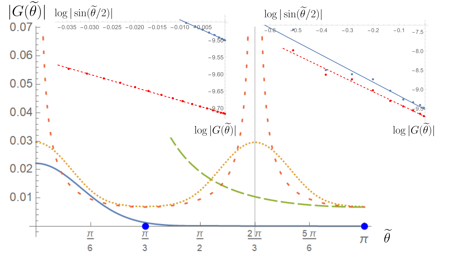
or, equivalently, |ρ~​(θ~)|∝|z−z′|−M|\widetilde{\rho}(\widetilde{\theta})|\propto|z-z^{\prime}|^{-M}. This is only valid in the vicinity of θ~=π\widetilde{\theta}=\pi (e.g., demanding the corrections to be ≤1%\leq 1\%, for M=3M=3, restricts us to [0.96​π,π][0.96\pi,\pi]), while Eq. (44) spans a broader range – see Fig. 3. The Green’s function was computed by using the tables of characters for permutation groups SN⁡(N−1)S_{N(N-1)} for M=3M=3 (up to N=8N=8 and then extrapolating the results), adjusting the method in Dunne 1993. The difference between |ρ||\rho| and |ρ~||\widetilde{\rho}| vanishes at π\pi as N−1/2N^{-1/2}.

Refer to caption
Figure 3: (Color online.) Edge Green’s function corresponding to the Laughlin’s (blue line) and the root (orange dotted line) state, for 8 particles. Both (sin⁡(θ~2))−3(\sin(\frac{\tilde{\theta}}{2}))^{-3} (green dashed line) and sin⁡(3​θ~2)\sin(\frac{3\tilde{\theta}}{2}) (red dashed line) laws are also shown. The latter is a better approximation of |ρ~||\widetilde{\rho}| in a broader range around π\pi. In the vicinity of blue points Stirling’s approximation is valid. Insets: log⁡|G⁡(θ~)|\log|G(\widetilde{\theta})| as a function of log⁡|sin⁡(θ~/2)|\log|\sin(\widetilde{\theta}/2)| in the range (Right): [0.6,1][0.6,1] for sin⁡(θ~/2)\sin(\widetilde{\theta}/2), for both N=8N=8 (red dashed line) and N=7N=7 (blue line); (Left): [0.967,1][0.967,1] for N=8N=8 (red dashed line) and [0.991,1][0.991,1] for N=7N=7 (blue line).

Nevertheless, the long-distance (θ~∼π\widetilde{\theta}\sim\pi) behavior of the Green’s function, in the thermodynamic limit, cannot be reliably determined from small NN calculations Wan et al. 2005. For instance, by examining the slope μ\mu of log⁡|G⁡(θ~)|\log|G(\widetilde{\theta})| when plotted as a function of log⁡|sin⁡(θ~/2)|\log|\sin(\widetilde{\theta}/2)| for N=8N=8 (Fig. 3), we get μ=−3.88\mu=-3.88 when using the range [0.967,1][0.967,1] for sin⁡(θ~/2)\sin(\widetilde{\theta}/2), while the value for N=7N=7 in the range [0.991,1][0.991,1] is μ=−6\mu=-6. The deduced numerical value is highly dependent on the range used in the fitting procedure, e.g. for N=8N=8 and the range [0.6,1][0.6,1] we obtain μ=−3.23\mu=-3.23 (for linear scale of θ~\widetilde{\theta}). We established that the asymptotic long-distance behavior of the edge Green’s function corresponding to the root state coincides with Wen’s conjecture Wen 1992.

VI.1 Beyond the LLL

The aforementioned behaviour remains true also beyond the LLL that forms the focus of our work. Indeed, repeating the above calculation when using the DNA Chen et al. 2017; Bandyopadhyay et al. 2018 of the Jain’s 2/52/5 state, we found μ=−3\mu=-3, in agreement with Wen’s hypothesis Wen 1992. In this Jain’s state example, our computation captures the (EPP) entanglement structure of the root partition Bandyopadhyay et al. 2018 not present in Laughlin states.

In this case we need the exact form of the following orbitals:

ψ0,r​(z)=zr𝒩0,r,ψ1,r​(z)=z∗​zr+1−2​(r+1)​zr𝒩1,r,\psi_{0,r}(z)=\frac{z^{r}}{\mathcal{N}_{0,r}},\qquad\psi_{1,r}(z)=\frac{{z}^{*}z^{r+1}-2(r+1)z^{r}}{\mathcal{N}_{1,r}}, (47)

with 𝒩0,r=2​π​2r​r!\mathcal{N}_{0,r}=\sqrt{2\pi 2^{r}r!} and 𝒩1,r=2​π​2r+2​(r+1)!\mathcal{N}_{1,r}=\sqrt{2\pi 2^{r+2}(r+1)!}. The fermionic field operator is now Ψ⁡(z)=∑n,rψn,r​(z)​c¯n,r\Psi(z)=\sum\limits_{n,r}\psi_{n,r}(z)\overline{c}_{n,r} which leads to the Green’s function of the following form:

ρ(z,z′)=∑n,n′∑r,r′ψn,r∗​(z)​ψn′,r′​(z′)​⟨ψ|c¯n,r†​c¯n′,r′|ψ⟩‖ψ‖2×e−14​(|z|2+|z′|2),\begin{split}\rho(z,z^{\prime})=\sum\limits_{n,n^{\prime}}\sum\limits_{r,r^{\prime}}&\psi_{n,r}^{\ast}(z)\psi_{n^{\prime},r^{\prime}}(z^{\prime})\frac{\langle\psi|\overline{c}^{\dagger}_{n,r}\overline{c}_{n^{\prime},r^{\prime}}|\psi\rangle}{\|\psi\|^{2}}\\ &\times e^{-\frac{1}{4}(|z|^{2}+|z^{\prime}|^{2})},\end{split} (48)

where |ψ⟩|\psi\rangle is the corresponding ground state. By the angular momentum conservation, r=r′r=r^{\prime} under the above summation, so that

ρ(z,z′)=∑n,n′∑rψn,r∗​(z)​ψn′,r​(z′)​⟨ψ|c¯n,r†​c¯n′,r|ψ⟩‖ψ‖2×e−14​(|z|2+|z′|2),\begin{split}\rho(z,z^{\prime})=\sum\limits_{n,n^{\prime}}\sum\limits_{r}&\psi_{n,r}^{\ast}(z)\psi_{n^{\prime},r}(z^{\prime})\frac{\langle\psi|\overline{c}^{\dagger}_{n,r}\overline{c}_{n^{\prime},r}|\psi\rangle}{\|\psi\|^{2}}\\ &\times e^{-\frac{1}{4}(|z|^{2}+|z^{\prime}|^{2})},\end{split} (49)

For the “DNA” of the ground state |ψ⟩|\psi\rangle we get

ρ~(z,z′)=∑n,n′∑rψn,r∗​(z)​ψn′,r​(z′)​⟨DNA|c¯n,r†​c¯n′,r|DNA⟩‖DNA‖2×e−14​(|z|2+|z′|2).\begin{split}\widetilde{\rho}(z,z^{\prime})=\sum\limits_{n,n^{\prime}}\sum\limits_{r}&\psi_{n,r}^{\ast}(z)\psi_{n^{\prime},r}(z^{\prime})\frac{\langle\mathrm{DNA}|\overline{c}^{\dagger}_{n,r}\overline{c}_{n^{\prime},r}|\mathrm{DNA}\rangle}{\|\mathrm{DNA}\|^{2}}\\ &\times e^{-\frac{1}{4}(|z|^{2}+|z^{\prime}|^{2})}.\end{split} (50)

The “DNA” of the ground state of the Jain’s 2/52/5 state Bandyopadhyay et al. 2018; Chen et al. 2017 is of the form |DNA⟩=∏k≥0φ5​k+3^​|0⟩|\mathrm{DNA}\rangle=\prod\limits_{k\geq 0}\widehat{\varphi_{5k+3}}|0\rangle with

φr^=α0,0​(r)(c¯0,r−1†​c¯0,r+1†+r+22​c¯0,r−1†​c¯1,r+1†CLOSEOPEN−r2​c¯1,r−1†​c¯0,r+1†),\begin{split}\widehat{\varphi_{r}}=\alpha_{0,0}(r)&\left(\overline{c}_{0,r-1}^{\dagger}\overline{c}_{0,r+1}^{\dagger}+\frac{\sqrt{r+2}}{2}\overline{c}_{0,r-1}^{\dagger}\overline{c}_{1,r+1}^{\dagger}\right.\\ &\left.-\frac{\sqrt{r}}{2}\overline{c}_{1,r-1}^{\dagger}\overline{c}_{0,r+1}^{\dagger}\right),\end{split} (51)

where α0,0\alpha_{0,0} is an rr-dependent factor.

As a result,

ρ~​(z,z′)=e−14​(|z|2+|z′|2)2​π×{∑0≤5​l+2≤rmax(z∗​z′)5​l+225​l+2​hl​(5​l+2)![1+(5l+5)2+2​(5​l+3)−|z′|24+(2(5l+3)−|z|2)(5l+3)]+∑0≤5​l+4≤rmax(z∗​z′)5​l+425​l+4​hl​(5​l+4)![1+(5l+3)2+|z′|2−2​(5​l+5)4+(|z|2−2(5l+5))(5l+5)]},\begin{split}&\widetilde{\rho}(z,z^{\prime})=\frac{e^{-\frac{1}{4}(|z|^{2}+|z^{\prime}|^{2})}}{2\pi}\\ &\times\left\{\sum\limits_{0\leq 5l+2\leq r_{\mathrm{max}}}\frac{({z}^{*}z^{\prime})^{5l+2}}{2^{5l+2}h_{l}(5l+2)!}\left[1+(5l+5)^{2}\right.\right.\\ &\left.\left.+\frac{2(5l+3)-|z^{\prime}|^{2}}{4}+(2(5l+3)-|z|^{2})(5l+3)\right]\right.\\ &\left.+\sum\limits_{0\leq 5l+4\leq r_{\mathrm{max}}}\frac{({z}^{*}z^{\prime})^{5l+4}}{2^{5l+4}h_{l}(5l+4)!}\left[1+(5l+3)^{2}\right.\right.\\ &\left.\left.+\frac{|z^{\prime}|^{2}-2(5l+5)}{4}+(|z|^{2}-2(5l+5))(5l+5)\right]\right\},\end{split} (52)

where hl=1+(5​l+3)2+(5​l+5)2h_{l}=1+(5l+3)^{2}+(5l+5)^{2}.

Henceforth, we will focus on points z=R​e𝗂​θz=Re^{{\sf i}\theta} and z′=R​e𝗂​θ′z^{\prime}=Re^{{\sf i}\theta^{\prime}} that lie on the edge. We next discuss the two contributions to ρ~​(z,z′)\widetilde{\rho}(z,z^{\prime}) in Eq. (52).

We start by discussing the contribution to ρ~​(z,z′)\widetilde{\rho}(z,z^{\prime}) of exponent 5​l+25l+2. With the above polar substitution for the boundary points zz and z′z^{\prime}, this becomes

e−12​R22​π​∑k=1𝒩(R22)5​(𝒩−k)+2​e−𝗂⁡(5​(𝒩−k)+2)​(θ−θ′)h𝒩−k​(5​(𝒩−k)+2)!×[1+(5(𝒩−k)+5)2+2​(5​(𝒩−k)+3)−R24⋅(20(𝒩−k)+13)],\begin{split}&\frac{e^{-\frac{1}{2}R^{2}}}{2\pi}\sum\limits_{k=1}^{\mathcal{N}}\left(\frac{R^{2}}{2}\right)^{5(\mathcal{N}-k)+2}\frac{e^{-{\sf i}(5(\mathcal{N}-k)+2)(\theta-\theta^{\prime})}}{h_{\mathcal{N}-k}\left(5(\mathcal{N}-k)+2\right)!}\\ &\times\left[1+\left(5(\mathcal{N}-k)+5\right)^{2}\right.\\ &\left.+\frac{2\left(5(\mathcal{N}-k)+3\right)-R^{2}}{4}\cdot(20(\mathcal{N}-k)+13)\right],\end{split} (53)

where 𝒩=⌊15​(N−1ν−2)⌋+1\mathcal{N}=\lfloor\frac{1}{5}\left(\frac{N-1}{\nu}-2\right)\rfloor+1 with ν=25\nu=\frac{2}{5}, and we have used the same change of summation index as in the case of the LLL.

Assume now that only small integer kk are of relevance in the above summation - we will check validity of this assumption later on. Then using the Stirling approximation, the fact that N≅R2​ν2≫1N\cong\frac{R^{2}\nu}{2}\gg 1 and 𝒩−k≅𝒩\mathcal{N}-k\cong\mathcal{N}, we get

[5​(𝒩−k)]!≅π​R​(R22)5​(𝒩−k)+2​e−R22,\left[5(\mathcal{N}-k)\right]!\cong\sqrt{\pi}R\left(\frac{R^{2}}{2}\right)^{5(\mathcal{N}-k)+2}e^{-\frac{R^{2}}{2}}, (54)

and, as a result, for the part with the exponent 5​l+25l+2, we end up with

e−𝗂​5​𝒩​(θ−θ′)2​R​π3/2​κ2​(𝒩,R)​∑k=1𝒩e𝗂⁡(5​k−2)​(θ−θ′),\frac{e^{-{\sf i}5\mathcal{N}(\theta-\theta^{\prime})}}{2R\pi^{3/2}}\kappa_{2}(\mathcal{N},R)\sum\limits_{k=1}^{\mathcal{N}}e^{{\sf i}(5k-2)(\theta-\theta^{\prime})}, (55)

where κ2​(𝒩,R)\kappa_{2}(\mathcal{N},R) is a certain rational function in 𝒩\mathcal{N}.

Similar to the above, for the part having 5​l+45l+4 as an exponent, we get

e−𝗂​5​𝒩^​(θ−θ′)2​R​π3/2​κ4​(𝒩^,R)​∑k=1𝒩^e𝗂⁡(5​k−4)​(θ−θ′)\frac{e^{-{\sf i}5\widehat{\mathcal{N}}(\theta-\theta^{\prime})}}{2R\pi^{3/2}}\kappa_{4}(\widehat{\mathcal{N}},R)\sum\limits_{k=1}^{\widehat{\mathcal{N}}}e^{{\sf i}(5k-4)(\theta-\theta^{\prime})} (56)

with a rational, in 𝒩^=⌊15​(N−1ν−4)⌋+1\widehat{\mathcal{N}}=\lfloor\frac{1}{5}\left(\frac{N-1}{\nu}-4\right)\rfloor+1, function κ4​(𝒩^,R)\kappa_{4}(\widehat{\mathcal{N}},R).

Next, we observe that for large radius RR we can without the loss of generality assume that 𝒩^=𝒩\widehat{\mathcal{N}}=\mathcal{N}, so that e−𝗂​5​𝒩^​(θ−θ′)e^{-{\sf i}5\widehat{\mathcal{N}}(\theta-\theta^{\prime})}’s lead to an irrelevant global factor since at the very end we will be interested in the absolute value of the Green’s function. We now argue that in the thermodynamic limit, κ2κ4→1\frac{\kappa_{2}}{\kappa_{4}}\rightarrow 1. Indeed, since R2∼2​NνR^{2}\sim\frac{2N}{\nu} and ν=25\nu=\frac{2}{5} we have R2∼5​NR^{2}\sim 5N. Moreover, we know that 𝒩∼N5​ν∼N2\mathcal{N}\sim\frac{N}{5\nu}\sim\frac{N}{2}. Hence R2∼10​𝒩R^{2}\sim 10\mathcal{N}. This shows that κ2κ4→1\frac{\kappa_{2}}{\kappa_{4}}\rightarrow 1. Furthermore, this also shows that, in the limit 𝒩→∞\mathcal{N}\rightarrow\infty, we have for ρ~\widetilde{\rho}:

e−𝗂​5​𝒩​(θ−θ′)4​R​π3/2​(∑k=1∞e𝗂⁡(5​k−2)​(θ−θ′)+∑k=1∞e𝗂⁡(5​k−4)​(θ−θ′)),\frac{e^{-{\sf i}5\mathcal{N}(\theta-\theta^{\prime})}}{4R\pi^{3/2}}\left(\sum\limits_{k=1}^{\infty}e^{{\sf i}(5k-2)(\theta-\theta^{\prime})}+\sum\limits_{k=1}^{\infty}e^{{\sf i}(5k-4)(\theta-\theta^{\prime})}\right), (57)

since both κ2\kappa_{2} and κ4\kappa_{4} tends to 12\frac{1}{2} in this limit.

We next explain why the assumption 𝒩−k≅𝒩\mathcal{N}-k\cong\mathcal{N} is valid. Towards this end, one needs to verify that the only kk values that matter are the small ones, i.e., that cos⁡((5​k−2)​(θ−θ′))≅(−1)k\cos((5k-2)(\theta-\theta^{\prime}))\cong(-1)^{k}. This is indeed true (in particular around θ−θ′=π\theta-\theta^{\prime}=\pi, which is exactly our point of interest). Analogous considerations work also for the term of exponent 5​l+45l+4. Therefore, the problem reduces to the evaluation of

14​R​π3/2​|∑k=1∞e𝗂⁡(5​k−2)​(θ−θ′)+e𝗂⁡(5​k−4)​(θ−θ′)|=14​R​π3/2​|𝗂​e𝗂​32​(θ−θ′)​cos⁡(θ−θ′)sin⁡(5​(θ−θ′)2)|.\begin{split}&\frac{1}{4R\pi^{3/2}}\left|\sum\limits_{k=1}^{\infty}e^{{\sf i}(5k-2)(\theta-\theta^{\prime})}+e^{{\sf i}(5k-4)(\theta-\theta^{\prime})}\right|\\ &=\frac{1}{4R\pi^{3/2}}\left|\frac{{\sf i}e^{{\sf i}\frac{3}{2}(\theta-\theta^{\prime})}\cos(\theta-\theta^{\prime})}{\sin\left(\frac{5(\theta-\theta^{\prime})}{2}\right)}\right|.\end{split} (58)

To ascertain the long distance behavior, we examine angular differences |θ−θ′|=θ~|\theta-\theta^{\prime}|=\tilde{\theta} close to π\pi, where this asymptotically becomes

14​R​π3/2​|1−2​sin2⁡(θ~2)sin⁡(5​θ~2)|≅12​R​π3/2​1|sin⁡(θ~2)|3.\begin{split}\frac{1}{4R\pi^{3/2}}\left|\frac{1-2\sin^{2}\left(\frac{\widetilde{\theta}}{2}\right)}{\sin\left(\frac{5\widetilde{\theta}}{2}\right)}\right|\cong\frac{1}{2R\pi^{3/2}}\frac{1}{\left|\sin\left(\frac{\widetilde{\theta}}{2}\right)\right|^{3}}.\end{split} (59)

The above derived result is in agreement with Wen’s conjecture Wen 1992 for the FQH Jain’s 2/52/5 liquid.

VII Conclusions

Our approach sheds light on the elusive exact mechanism underlying fractionalized quasielectron excitations in FQH fluids (and formalizes the fractionalization of quasihole excitations Girvin 1984). By solving an outstanding open problem Kjäll et al. 2018; Nielsen et al. 2018, our construct underscores the importance of a systematic operator based microscopic approach complementing Laughlin’s original quasiparticle wave function Ansatz. The algebraic structure of the LLL is deeply tied to the Newton-Girard relations. We have shown that there are numerous pairs of “dual” operators that are linked to each other via these relations (including operators associated with the Witt algebra). The Newton-Girard relations typically convert a local operator into a non-local “dual” operator. A main message of the present work is that “derivative operations” on FQH vacua do not lead to exact quasiparticle excitations. The precise mechanism leading to charge fractionalization consists of the joint process of flux and (original) particle insertions. In other words, an elementary fusion channel of quasiholes and an electron generates a quasielectron excitation. For instance, to generate one quasielectron excitation in a ν=1/M\nu=1/M Laughlin fluid one needs to insert M−1M-1 fluxes, in an (N−1N-1)-electron fluid, and fuse them with an additional electron. A fundamental difference between quasihole and quasiparticle excitations can be traced back to their MM-clustering properties Bandyopadhyay et al. 2018. While quasiholes preserve the MM-clustering property of the incompressible (ground state) fluid, quasiparticle states breaks it down. This is at the origin of the asymmetry between these two kinds of excitations. Equivalently, while quasihole wave functions sustain a (local) plasma analogy this is not the case for quasielectrons.

We explicitly constructed the quasiparticle (quasielectron) wave function. Our found fusion mechanism of quasiparticle generation is not only the mathematically exact (for an arbitrary number of particles) field-theoretic operator procedure but it is also behind the exact analytic computation of other quasiparticle properties, such as its charge density and Berry connections leading to the right fractional charge and exchange statistics. This is a truly unprecedented remarkable result that we have numerically confirmed via detailed Monte Carlo simulations.

Intriguingly, within our field-theoretic framework, we find that the Laughlin state is a condensate of a non-local Read type operator. Our approach allows for a constructive (zero-energy) subspace bosonization of the full two-dimensional system that further evinces the non-local topological character of the problem and, once again, cements links to Read’s operator. The constructed Klein operator associated with this angular momentum (and flux counting) root state based bosonization scheme is none other than Read’s non-local operator. We suspect that this angular momentum (flux counting) based mapping might relate to real-space flux attachment (and attendant Chern-Simons) type bosonization schemes Fradkin 2013; Seiberg et al. 2016. Lastly, we illustrated how the long-distance behavior of edge excitations associated with the root partition component (DNA) of the bulk FQH ground state may be readily calculated. Strikingly, the asymptotic long-distance edge physics derived in this manner matches Wen’s earlier hypothesis in the cases that we tested. This agreement hints at a possibly general powerful computational recipe for predicting edge physics.

VIII Acknowledgements

We thank J. Jain, H. Hansson, and S. Simon for useful comments. G.O. acknowledges support from the US Department of Energy grant DE-SC0020343. A.B. acknowledges the Polish-US Fulbright Commission for the possibility of visiting Indiana University, Bloomington, during the Fulbright Junior Research Award scholarship. Work by A.S. has been supported by the National Science Foundation Grant No. DMR-2029401.

References

  • Jain (2007) J. K. Jain, Composite Fermions (Cambridge University Press, 2007).
  • Bandyopadhyay et al. (2018) S. Bandyopadhyay, L. Chen, M. T. Ahari, G. Ortiz, Z. Nussinov, and A. Seidel, Entangled pauli principles: The dna of quantum hall fluids, Phys. Rev. B 98, 161118 (2018).
  • Bernevig and Haldane (2008) B. A. Bernevig and F. D. M. Haldane, Model fractional quantum hall states and jack polynomials, Phys. Rev. Lett. 100, 246802 (2008).
  • Ortiz et al. (2013) G. Ortiz, Z. Nussinov, J. Dukelsky, and A. Seidel, Repulsive interactions in quantum hall systems as a pairing problem, Phys. Rev. B 88, 165303 (2013).
  • Laughlin (1983) R. B. Laughlin, Anomalous quantum hall effect: An incompressible quantum fluid with fractionally charged excitations, Phys. Rev. Lett. 50, 1395 (1983).
  • (6) One can always apply a similarity transformation to map to the cylinder Ortiz et al. 2013.
  • (7) Normalization is defined as ∫𝒟⁡[z]​(z∗)r​zr′=𝒩r2​δr,r′\intop\nolimits{\cal D}[z](z^{*})^{r}z^{r^{\prime}}={\cal N}_{r}^{2}\delta_{r,r^{\prime}} with 𝒟⁡[z]=d2​z​e−12​|z|2{\cal D}[z]=d^{2}ze^{-\frac{1}{2}|z|^{2}}, z∗=x−𝗂​yz^{*}=x-{\sf i}y, and magnetic unit length ℓ=1\ell=1.
  • Stone (1992) M. Stone, Quantum Hall Effect (World Scientific, Singapore, 1992) Chap. 4.
  • Mazaheri et al. (2015) T. Mazaheri, G. Ortiz, Z. Nussinov, and A. Seidel, Zero modes, bosonization, and topological quantum order: The laughlin state in second quantization, Phys. Rev. B 91, 085115 (2015).
  • Cobanera et al. (2010) E. Cobanera, G. Ortiz, and Z. Nussinov, Unified approach to quantum and classical dualities, Phys. Rev. Lett. 104, 020402 (2010).
  • Cobanera et al. (2011) E. Cobanera, G. Ortiz, and Z. Nussinov, The bond-algebraic approach to dualities, Advances in Physics 60, 679 (2011).
  • Nussinov et al. (2015) Z. Nussinov, G. Ortiz, and M.-S. Vaezi, Why are all dualities conformal? theory and practical consequences, Nuclear Physics B 892, 132 (2015).
  • Bandyopadhyay et al. (2020) S. Bandyopadhyay, G. Ortiz, Z. Nussinov, and A. Seidel, Local two-body parent hamiltonians for the entire jain sequence, Phys. Rev. Lett. 124, 196803 (2020).
  • (14) We remark that in Stone 1992 orbitals ϕr​(z)\phi_{r}(z) include Gaussian factors in contrast to our convention. That implies a change in the differential operator to D(z)=2∂z∗+12zD^{(z)}=2\partial_{z^{\ast}}+\frac{1}{2}z.
  • Read (1989) N. Read, Order parameter and ginzburg-landau theory for the fractional quantum hall effect, Phys. Rev. Lett. 62, 86 (1989).
  • (16) In first-quantization language this first appeared in Girvin 1984 and an early discussion in Anderson 1983. For a rigorous and general proof of Eq. (7) see Appendix D.
  • Girvin and MacDonald (1987) S. M. Girvin and A. H. MacDonald, Off-diagonal long-range order, oblique confinement, and the fractional quantum hall effect, Phys. Rev. Lett. 58, 1252 (1987).
  • Chen et al. (2019) L. Chen, S. Bandyopadhyay, K. Yang, and A. Seidel, Composite fermions in fock space: Operator algebra, recursion relations, and order parameters, Phys. Rev. B 100, 045136 (2019).
  • (19) In first quantization the Gaussian factor is typically not included in the integration measure.
  • Hansson et al. (2017) T. H. Hansson, M. Hermanns, S. H. Simon, and S. F. Viefers, Quantum hall physics: Hierarchies and conformal field theory techniques, Rev. Mod. Phys. 89, 025005 (2017).
  • Jeon and Jain (2003) G. S. Jeon and J. K. Jain, Nature of quasiparticle excitations in the fractional quantum hall effect, Phys. Rev. B 68, 165346 (2003).
  • Kjäll et al. (2018) J. Kjäll, E. Ardonne, V. Dwivedi, M. Hermanns, and T. H. Hansson, Matrix product state representation of quasielectron wave functions, J. Stat. Mech. 2018, 053101 (2018).
  • Nielsen et al. (2018) A. E. B. Nielsen, I. Glasser, and I. D. Rodríguez, Quasielectrons as inverse quasiholes in lattice fractional quantum hall model, New J. Phys. 20, 033029 (2018).
  • MacDonald and Girvin (1986) A. H. MacDonald and S. M. Girvin, Quasiparticle states in the fractional quantum hall effect, Phys. Rev. B 34, 5639 (1986).
  • Arovas et al. (1984) D. Arovas, J. R. Schrieffer, and F. Wilczek, Fractional statistics and the quantum hall effect, Phys. Rev. Lett. 53, 722 (1984).
  • Rigolin et al. (2008) G. Rigolin, G. Ortiz, and V. H. Ponce, Beyond the quantum adiabatic approximation: Adiabatic perturbation theory, Phys. Rev. A 78, 052508 (2008).
  • Rigolin and Ortiz (2010) G. Rigolin and G. Ortiz, Adiabatic perturbation theory and geometric phases for degenerate systems, Phys. Rev. Lett. 104, 170406 (2010).
  • Ortiz et al. (1993) G. Ortiz, D. M. Ceperley, and R. M. Martin, New stochastic method for systems with broken time-reversal symmetry: 2d fermions in a magnetic field, Phys. Rev. Lett. 71, 2777 (1993).
  • Kivelson and Schrieffer (1982) S. Kivelson and J. R. Schrieffer, Fractional charge, a sharp quantum observable, Phys. Rev. B 25, 6447 (1982).
  • Su (1986) W. P. Su, Statistics of the fractionally charged excitations in the quantum hall effect, Phys. Rev. B 34, 1031 (1986).
  • Delft and Schoeller (1998) J. Delft and H. Schoeller, Bosonization for beginners — refermionization for experts, Annalen der Physik 7, 225 (1998).
  • Seiberg et al. (2016) N. Seiberg, T. Senthil, C. Wang, and E. Witten, A duality web in 2+1 dimensions and condensed matter physics, Annals of Physics 374, 395 (2016).
  • Fuentes et al. (1995) M. Fuentes, A. Lopez, E. Fradkin, and E. Moreno, Bosonization rules in 1/2+1 dimensions, Nuclear Physics B 450, 603 (1995).
  • Wen (1992) X.-G. Wen, Theory of the edge states in fractional quantum hall effects, International Journal of Modern Physics B 06, 1711 (1992), https://doi.org/10.1142/S0217979292000840 .
  • Fern et al. (2018) R. Fern, R. Bondesan, and S. H. Simon, Effective edge state dynamics in the fractional quantum hall effect, Phys. Rev. B 98, 155321 (2018).
  • Mandal and Jain (2001) S. S. Mandal and J. K. Jain, How universal is the fractional-quantum-hall edge luttinger liquid?, Solid State Communications 118, 503 (2001).
  • Dunne (1993) G. V. Dunne, Slater decomposition of Laughlin states, International Journal of Modern Physics B 07, 4783 (1993).
  • Wan et al. (2005) X. Wan, F. Evers, and E. H. Rezayi, Universality of the edge-tunneling exponent of fractional quantum hall liquids, Phys. Rev. Lett. 94, 166804 (2005).
  • Chen et al. (2017) L. Chen, S. Bandyopadhyay, and A. Seidel, Jain-2/5 parent hamiltonian: Structure of zero modes, dominance patterns, and zero mode generators, Phys. Rev. B 95, 195169 (2017).
  • Girvin (1984) S. M. Girvin, Particle-hole symmetry in the anomalous quantum hall effect, Phys. Rev. B 29, 6012 (1984).
  • Fradkin (2013) E. Fradkin, Field Theories of Condensed Matter Physics, 2nd ed. (Cambridge University Press, 2013).
  • Anderson (1983) P. W. Anderson, Remarks on the laughlin theory of the fractionally quantized hall effect, Phys. Rev. B 28, 2264 (1983).
  • MacDonald (1995) I. G. MacDonald, Symmetric Functions and Hall Polynomials, 2nd ed. (Oxford University Press, 1995).
  • Comtet (1970) L. Comtet, Analyse combinatoire, Vol. 1 (Presses Universitaires de France, 1970).
  • Chen and Seidel (2015) L. Chen and A. Seidel, Algebraic approach to the study of zero modes of haldane pseudopotentials, Phys. Rev. B 91, 085103 (2015).
  • (46) The analogous statement is in those cases also true for higher values of MM.

Appendix A Newton-Girard dual pairs

Let d≥0d\geq 0, and consider operators 𝒪d\mathcal{O}_{d} and ede_{d}, defined for both fermions and bosons. Since they are operator analogues of the symmetric polynomials pd​(z)=∑i=1Nzidp_{d}(z)=\sum\limits_{i=1}^{N}z_{i}^{d} and sd​(z)=∑1≤i1≤…≤id≤Nzi1​…​zids_{d}(z)=\sum\limits_{1\leq i_{1}\leq\ldots\leq i_{d}\leq N}z_{i_{1}}\ldots z_{i_{d}}, respectively, one may expect that the operator version of the Netwon-Girard relation, known from the theory of symmetric polynomials, holds also in this case:

d​ed+∑k=1d(−1)k​𝒪k​ed−k=0.de_{d}+\sum\limits_{k=1}^{d}(-1)^{k}\mathcal{O}_{k}e_{d-k}=0. (60)

Indeed, this was already proven in Mazaheri et al. 2015. Then, 𝒪d\mathcal{O}_{d} operators can be expressed recursively in terms of ede_{d}’s:

𝒪d=(−1)d−1​(d​ed+∑k=1d−1(−1)k​𝒪k​ed−k),\mathcal{O}_{d}=(-1)^{d-1}\left(de_{d}+\sum\limits_{k=1}^{d-1}(-1)^{k}\mathcal{O}_{k}e_{d-k}\right), (61)

so that any operator 𝒪d\mathcal{O}_{d} can be represented in terms of ede_{d}’s only, and vice versa. Moreover, this can be achieved by a (many-variable) polynomial relation. In order to write an explicit expression for 𝒪d\mathcal{O}_{d} in terms of ede_{d}’s operators we start with the Newton-Girard relation, (60), and for any positive dd we get

{e1=𝒪1,2​e2=e1​𝒪1−𝒪2,d​ed=ed−1​𝒪1−ed−2​𝒪2+…+(−1)d​e1​𝒪d−1+(−1)d−1​𝒪d.\begin{cases}e_{1}=\mathcal{O}_{1},\\ 2e_{2}=e_{1}\mathcal{O}_{1}-\mathcal{O}_{2},\\ \vdots\\ de_{d}=e_{d-1}\mathcal{O}_{1}-e_{d-2}\mathcal{O}_{2}+\ldots+(-1)^{d}e_{1}\mathcal{O}_{d-1}\\ \hskip 129.74449pt+(-1)^{d-1}\mathcal{O}_{d}.\end{cases} (62)

Since, again by the Newton-Girard relation, every coefficient which is a multiple of eke_{k} is also in the algebra 𝖠\mathsf{A} of 𝒪d\mathcal{O}_{d} operators, this leads to a system of dd linear equations in the commutative algebra 𝖠\mathsf{A}. We would like to solve this linear system for unknowns (𝒪1,−𝒪2,𝒪3,…,(−1)d​𝒪d−1,𝒪d)(\mathcal{O}_{1},-\mathcal{O}_{2},\mathcal{O}_{3},\ldots,(-1)^{d}\mathcal{O}_{d-1},\mathcal{O}_{d}). By Cramer’s theorem applied to the ring 𝖠\mathsf{A}, the necessary and sufficient condition for the existence of the unique solution is the invertibility in 𝖠\mathsf{A} of the determinant of the matrix encoding this system. In our case this is a lower triangular matrix with diagonal (1,…,1⏟d−1,(−1)d−1)(\underbrace{1,\ldots,1}_{d-1},(-1)^{d-1}), so its determinant, equal to (−1)d−1(-1)^{d-1}, is clearly an invertible element in 𝖠\mathsf{A}. Therefore, again by Cramer’s theorem, we get (see also (MacDonald 1995, p. 28)):

𝒪d\displaystyle\mathcal{O}_{d} =\displaystyle= (−1)d−1​det(100…0e1e110…02​e2e2e11…03​e3⋱ed−2ed−3ed−4…1(d−1)​ed−1ed−1ed−2ed−3…e1d​ed)\displaystyle(-1)^{d-1}\det\!\!\begin{pmatrix}1&0&0&\ldots&0&e_{1}\\ e_{1}&1&0&\ldots&0&2e_{2}\\ e_{2}&e_{1}&1&\ldots&0&3e_{3}\\ \vdots&\vdots&\vdots&\ddots&\vdots&\vdots\\ e_{d-2}&e_{d-3}&e_{d-4}&\ldots&1&(d-1)e_{d-1}\\ e_{d-1}&e_{d-2}&e_{d-3}&\ldots&e_{1}&de_{d}\end{pmatrix}
=\displaystyle= det(e1100…02​e2e110…03​e3e2e11…0⋱d​eeed−1ed−2ed−3…e1).\displaystyle\det\begin{pmatrix}e_{1}&1&0&0&\ldots&0\\ 2e_{2}&e_{1}&1&0&\ldots&0\\ 3e_{3}&e_{2}&e_{1}&1&\ldots&0\\ \vdots&\vdots&\vdots&\vdots&\ddots&\vdots\\ de_{e}&e_{d-1}&e_{d-2}&e_{d-3}&\ldots&e_{1}\end{pmatrix}.

Expanding the above determinant one can finally find

𝒪d\displaystyle\mathcal{O}_{d} =\displaystyle= (−1)d​d​∑r1+2​r2+…+d​rd=dr1,…,rd≥0(r1+…+rd−1)!r1!​…​r2!\displaystyle(-1)^{d}d\sum\limits_{\begin{subarray}{c}r_{1}+2r_{2}+\ldots+dr_{d}=d\\ r_{1},\ldots,r_{d}\geq 0\end{subarray}}\frac{(r_{1}+\ldots+r_{d}-1)!}{r_{1}!\ldots r_{2}!} (63)
×(−1)r1+…+rd​e1r1​…​edrd\displaystyle\hskip 85.35826pt\times(-1)^{r_{1}+\ldots+r_{d}}e_{1}^{r_{1}}\ldots e_{d}^{r_{d}}
=\displaystyle= (−1)d​d​∑k=1d1k​B^d,k​(−e1,…,−ed−k−1),\displaystyle(-1)^{d}d\sum\limits_{k=1}^{d}\frac{1}{k}\hat{B}_{d,k}(-e_{1},\ldots,-e_{d-k-1}),

where B^n,k​(x1,…,xn−k+1)=k!n!​Bn,k​(1!​x1,2!​x2,…,(n−k+1)!​xn−k+1)\hat{B}_{n,k}(x_{1},\ldots,x_{n-k+1})=\frac{k!}{n!}B_{n,k}(1!x_{1},2!x_{2},\ldots,(n-k+1)!x_{n-k+1}) and Bn,kB_{n,k} is the (exponential) Bell polynomial Comtet 1970.

Let now fdf_{d} be the operator representing, in the second quantization picture, the elementary symmetric polynomial with the ziz_{i} variables substituted by partial derivatives, sd(∂z)s_{d}(\partial_{z}), and let 𝒬d\mathcal{Q}_{d} be the second-quantized version of the operator pd(∂z)p_{d}(\partial_{z}). Since the Newton-Girard relation holds for sd(∂z)s_{d}(\partial_{z}) and pd(∂z)p_{d}(\partial_{z}), an analogous one is expected for the pair of operators fdf_{d} and 𝒬d\mathcal{Q}_{d}.

First, we claim that the second-quantized version fdf_{d} of the differential operator sd(∂z)s_{d}(\partial_{z}) is

fd=1d!​∑r1,…,rd>0r1​…​rd​a¯r1−1†​…​a¯rd−1†​a¯rd​…​a¯r1.f_{d}=\frac{1}{d!}\sum\limits_{r_{1},\ldots,r_{d}>0}r_{1}\ldots r_{d}\,\overline{a}_{r_{1}-1}^{\dagger}\ldots\overline{a}_{r_{d}-1}^{\dagger}\overline{a}_{r_{d}}\ldots\overline{a}_{r_{1}}. (64)

We start with the fermionic case. For β1>…>βN≥0\beta_{1}>\ldots>\beta_{N}\geq 0 consider the monic monomial rβ​(ZN)=z1β1​…​zNβNr_{\beta}(Z_{N})=z_{1}^{\beta_{1}}\ldots z_{N}^{\beta_{N}}, where β=(β1,…,βN)\beta=(\beta_{1},\ldots,\beta_{N}) and ZN=(z1,…,zN)Z_{N}=(z_{1},\ldots,z_{N}). rβr_{\beta} is a homogeneous polynomial of degree |β|=β1+…+βN|\beta|=\beta_{1}+\ldots+\beta_{N}. Let Rβ​(ZN)=N!​𝒜^​rβ​(ZN)R_{\beta}(Z_{N})=N!\widehat{\mathcal{A}}r_{\beta}(Z_{N}) be defined by the total antisymmetrization 𝒜^\widehat{\mathcal{A}} of rβr_{\beta} in variables forming ZNZ_{N}. This polynomial corresponds, in second quantization, to the operator 𝔠¯β†=c¯β1†​…​c¯βN†\overline{\mathfrak{c}}_{\beta}^{\dagger}=\overline{c}_{\beta_{1}}^{\dagger}\ldots\overline{c}_{\beta_{N}}^{\dagger}, the Slater determinant.

Notice that for d>Nd>N, fd​𝔠¯β=0f_{d}\overline{\mathfrak{c}}_{\beta}=0, and similarly sd(∂z)Rd(ZN)=0s_{d}(\partial_{z})R_{d}(Z_{N})=0. Therefore, below we implicitly assume that dd is at most NN. We notice that

sd(∂z)Rβ(ZN)\displaystyle s_{d}(\partial_{z})R_{\beta}(Z_{N}) =\displaystyle= N!𝒜^sd(∂z)rβ(ZN)\displaystyle N!\widehat{\mathcal{A}}s_{d}(\partial_{z})r_{\beta}(Z_{N}) (65)
=N!​𝒜^​𝒮(i1,…​id)​(∂zi1…​∂zidz1β1​…​zNβN)\displaystyle\hskip-71.13188pt=N!\widehat{\mathcal{A}}\mathcal{S}_{(i_{1},\ldots i_{d})}\left(\partial_{z_{i_{1}}}\ldots\partial_{z_{i_{d}}}z_{1}^{\beta_{1}}\ldots z_{N}^{\beta_{N}}\right)
=N!​𝒜^​𝒮(i1,…​id)​(βi1​…​βid​z1β1​…​zi1βi1−1​…​zidβid−1​…​zNβN)\displaystyle\hskip-71.13188pt=N!\widehat{\mathcal{A}}\mathcal{S}_{(i_{1},\ldots i_{d})}\left(\beta_{i_{1}}\ldots\beta_{i_{d}}z_{1}^{\beta_{1}}\ldots z_{i_{1}}^{\beta_{i_{1}}-1}\ldots z_{i_{d}}^{\beta_{i_{d}}-1}\ldots z_{N}^{\beta_{N}}\right)
=𝒮(i1,…​id)​(βi1​…​βid​R(β1,…,βi1−1,…,βid−1,…,βN)​(z)).\displaystyle\hskip-71.13188pt=\mathcal{S}_{(i_{1},\ldots i_{d})}\left(\beta_{i_{1}}\ldots\beta_{i_{d}}R_{(\beta_{1},\ldots,\beta_{i_{1}}-1,\ldots,\beta_{i_{d}-1},\ldots,\beta_{N})}(z)\right).

Here 𝒮(i1,…,id)\mathcal{S}_{(i_{1},\ldots,i_{d})} denotes the total symmetrization in i1,…,idi_{1},\ldots,i_{d} with ij≠iki_{j}\neq i_{k} for every pair (j,k)(j,k) of indices j,k∈{1,…,d}j,k\in\{1,\ldots,d\} such that j≠kj\neq k.

Observe that when acting by the operator fdf_{d} on the state 𝔠¯β†​|0⟩\overline{\mathfrak{c}}_{\beta}^{\dagger}|0\rangle the symmetrization 𝒮(i1,…​id)\mathcal{S}_{(i_{1},\ldots i_{d})} is explicitly involved. Moreover, each term under the symmetrization produces

βi1​…​βid​c¯βi1−1†​…​c¯βid−1†​c¯βid​…​c¯βi1​c¯β1†​…​c¯βN†​|0⟩.\beta_{i_{1}}\ldots\beta_{i_{d}}\overline{c}_{\beta_{i_{1}}-1}^{\dagger}\ldots\overline{c}_{\beta_{i_{d}}-1}^{\dagger}\overline{c}_{\beta_{i_{d}}}\ldots\overline{c}_{\beta_{i_{1}}}\overline{c}_{\beta_{1}}^{\dagger}\ldots\overline{c}_{\beta_{N}}^{\dagger}|0\rangle. (66)

To finish the proof it is enough to show that when placing the fermionic operators in the canonical order no sign is generated out of the reordering permutation. By counting signs appearing in the reordering, one can easily check that this is indeed the case.

For bosons, in the definition of Rβ​(ZN)R_{\beta}(Z_{N}) we replace the total antisymmetrization by a symmetrization, which corresponds to having a permament instead of a Slater determinant. The reasoning in (65) follows with only minor adjustments. Now 𝒮(i1,…,id)\mathcal{S}_{(i_{1},\ldots,i_{d})} denotes the total symmetrization in i1,…,idi_{1},\ldots,i_{d} without the additional assumption that the indices are pairwise distinct, contrary to the fermionic case. Obviously, no sign counting in the reordering is needed in the bosonic case.

In order to justify that 𝒬d=∑r>0r⁡(r−1)​…​(r−d)​a¯r−d†​a¯r\mathcal{Q}_{d}=\sum\limits_{r>0}r(r-1)\ldots(r-d)\overline{a}_{r-d}^{\dagger}\overline{a}_{r} is the second-quantized version of the pd(∂z)p_{d}(\partial_{z}) polynomial, we will show that this operator satisfies the Newton-Girard equation. First notice that mimicking the computation from Mazaheri et al. 2015 one can easily prove that

[fd,a¯r†]−=r​a¯r−1†​fd−1,[fd,a¯r]−=−(r+1)​fd−1​a¯r−1,[f_{d},\overline{a}_{r}^{\dagger}]_{-}=r\overline{a}_{r-1}^{\dagger}f_{d-1},\qquad[f_{d},\overline{a}_{r}]_{-}=-(r+1)f_{d-1}\overline{a}_{r-1}, (67)

for any d>0d>0 and r≥0r\geq 0. Moreover, we have

fd=1d​∑r≥0r​a¯r−1†​fd−1​a¯r.\begin{split}f_{d}&=\frac{1}{d}\sum\limits_{r\geq 0}r\overline{a}^{\dagger}_{r-1}f_{d-1}\overline{a}_{r}.\end{split} (68)

Next, iterating this equation sufficiently many times we find (f1=𝒬1f_{1}=\mathcal{Q}_{1})

d​fd=∑r≥0r⁡(fd−1​a¯r−1†−(r−1)​a¯r−2†​fd−2)​a¯r=fd−1​𝒬1−∑r≥0r⁡(r−1)​a¯r−2†​fd−2​a¯r=fd−1​𝒬1−∑r≥0r⁡(r−1)​(fd−2​a¯r−2†−(r−2)​a¯r−3†​fd−3)=fd−1​𝒬1+(−1)​fd−2​𝒬2+(−1)2∑r≥0r(r−1)(r−2)a¯r−3†fd−3=…=−∑k=1d(−1)kfd−k𝒬k.\begin{split}df_{d}&=\sum\limits_{r\geq 0}r\left(f_{d-1}\overline{a}_{r-1}^{\dagger}-(r-1)\overline{a}_{r-2}^{\dagger}f_{d-2}\right)\overline{a}_{r}\\ &=f_{d-1}\mathcal{Q}_{1}-\sum\limits_{r\geq 0}r(r-1)\overline{a}_{r-2}^{\dagger}f_{d-2}\overline{a}_{r}\\ &=f_{d-1}\mathcal{Q}_{1}\!-\!\sum\limits_{r\geq 0}r(r-1)\!\!\left(f_{d-2}\overline{a}_{r-2}^{\dagger}-(r-2)\overline{a}_{r-3}^{\dagger}f_{d-3}\right)\\ &=f_{d-1}\mathcal{Q}_{1}+(-1)f_{d-2}\mathcal{Q}_{2}\\ &\hskip 45.52458pt+(-1)^{2}\sum\limits_{r\geq 0}r(r-1)(r-2)\overline{a}_{r-3}^{\dagger}f_{d-3}\\ &=\ldots=-\sum\limits_{k=1}^{d}(-1)^{k}f_{d-k}\mathcal{Q}_{k}.\end{split} (69)

By induction, each fdf_{d} commutes with every 𝒬k\mathcal{Q}_{k}, so that we end up with the Newton-Girard relation for the operators fdf_{d} and 𝒬k\mathcal{Q}_{k}:

d​fd+∑k=1d(−1)k​𝒬k​fd−k=0.df_{d}+\sum\limits_{k=1}^{d}(-1)^{k}\mathcal{Q}_{k}f_{d-k}=0. (70)

A.1 The Witt algebra

For d≥0d\geq 0 we consider also the differential operators ℓd=−∑i=1Nzid+1∂zi\ell_{d}=-\sum\limits_{i=1}^{N}z_{i}^{d+1}\partial_{z_{i}}. They satisfy [ℓd,ℓd′]−=(d−d′)​ℓd+d′[\ell_{d},\ell_{d^{\prime}}]_{-}=(d-d^{\prime})\ell_{d+d^{\prime}}, i.e. form the positive Witt algebra 𝔚+\mathfrak{W}_{+}. Another set of operators satisfying the same algebra is given by ℓ^d=−∑r≥0ra¯r+d†a¯r\widehat{\ell}_{d}=-\sum\limits_{r\geq 0}r\overline{a}_{r+d}^{\dagger}\overline{a}_{r}. We claim that ℓ^d\widehat{\ell}_{d} is the second quantization version of ℓd\ell_{d}. Indeed, we will show it explicitly for fermions and left the adjustments in the bosonic case to the reader as they are exactly the same as we discussed above in the case of the fdf_{d} operator. We have ℓdrβ(ZN)=−∑i=1Nβiz1β1…ziβi+d…zNβN\ell_{d}r_{\beta}(Z_{N})=-\sum\limits_{i=1}^{N}\beta_{i}z_{1}^{\beta_{1}}\ldots z_{i}^{\beta_{i}+d}\ldots z_{N}^{\beta_{N}}. Since ℓd\ell_{d} is symmetric under transpositions (i,j)(i,j) for any two indices i,ji,j under the summation, from the very definition of the totally antisymmetrized polynomial Rβ​(ZN)R_{\beta}(Z_{N}) we have also that ℓd​Rβ​(ZN)=N!​𝒜^​ℓd​rβ​(ZN)\ell_{d}R_{\beta}(Z_{N})=N!\widehat{\mathcal{A}}\ell_{d}r_{\beta}(Z_{N}), and, as a result, we end up with ℓdRβ(ZN)=−∑j=1NβjR(β1,…,βj−1,βj+d,βj+1,…,βN)(ZN)\ell_{d}R_{\beta}(Z_{N})=-\sum\limits_{j=1}^{N}\beta_{j}R_{(\beta_{1},\ldots,\beta_{j-1},\beta_{j}+d,\beta_{j+1},\ldots,\beta_{N})}(Z_{N}). On the other hand, for the Slater determinant corresponding to the polynomial Rβ​(ZN)R_{\beta}(Z_{N}) we have ℓ^d​𝔠¯β†​|0⟩=∑j=1Nβj​c¯β1†​…​c¯βj−1†​c¯βj+d†​c¯βj+1†​…​c¯βN†​|0⟩\widehat{\ell}_{d}\overline{\mathfrak{c}}_{\beta}^{\dagger}|0\rangle=\sum\limits_{j=1}^{N}\beta_{j}\overline{c}_{\beta_{1}}^{\dagger}\ldots\overline{c}_{\beta_{j-1}}^{\dagger}\overline{c}_{\beta_{j}+d}^{\dagger}\overline{c}_{\beta_{j+1}}^{\dagger}\ldots\overline{c}_{\beta_{N}}^{\dagger}|0\rangle, where we have used the fact that the total number of transpositions required to properly order the creation operators is even. It remains to notice that the Slater determinant cβ1†​…​c¯βj−1†​c¯βj+d†​c¯βj+1†​…​c¯βN†c_{\beta_{1}}^{\dagger}\ldots\overline{c}_{\beta_{j-1}}^{\dagger}\overline{c}_{\beta_{j}+d}^{\dagger}\overline{c}_{\beta_{j+1}}^{\dagger}\ldots\overline{c}_{\beta_{N}}^{\dagger} corresponds to the polynomial R(β1,…,βj−1,βj+d,βj+1,…,βN)​(ZN)R_{(\beta_{1},\ldots,\beta_{j-1},\beta_{j}+d,\beta_{j+1},\ldots,\beta_{N})}(Z_{N}).

Appendix B Properties of the quasihole operator

The quasihole operator U^N​(η)=∑d=0N(−η)N−d​ed\widehat{U}_{N}(\eta)=\sum\limits_{d=0}^{N}(-\eta)^{N-d}e_{d} satisfies the following important relations:

U^N​(η)​a¯r†=−η​a¯r†​U^N​(η)+a¯r+1†​U^N​(η),\widehat{U}_{N}(\eta)\overline{a}_{r}^{\dagger}=-\eta\overline{a}_{r}^{\dagger}\widehat{U}_{N}(\eta)+\overline{a}_{r+1}^{\dagger}\widehat{U}_{N}(\eta), (71)
a¯r​U^N​(η)=−η​U^N​(η)​a¯r+U^N​(η)​a¯r−1.\overline{a}_{r}\widehat{U}_{N}(\eta)=-\eta\widehat{U}_{N}(\eta)\overline{a}_{r}+\widehat{U}_{N}(\eta)\overline{a}_{r-1}. (72)

Since the first of those relations was already demonstrated in Mazaheri et al. 2015, we present here, for completeness, the proof of the second one. This follows as a result of a straightforward computation:

U^N​(η)​a¯r=(−η)N^​∑d≥0(−η)−d​ed​a¯r=(−η)N^​∑d≥0(−ed−1​a¯r−1+a¯r​ed)=−(−η)N^(−η)−1∑d≥0(−η)−d−1ed−1a¯r−1+a¯r(−η)−1(η)N^∑d≥0(−η)−ded=1η​U^N​(η)​a¯r−1−1η​a¯r​U^N​(η).\begin{split}\widehat{U}_{N}(\eta)\overline{a}_{r}&=(-\eta)^{\widehat{N}}\sum\limits_{d\geq 0}(-\eta)^{-d}e_{d}\overline{a}_{r}\\ &=(-\eta)^{\widehat{N}}\sum\limits_{d\geq 0}(-e_{d-1}\overline{a}_{r-1}+\overline{a}_{r}e_{d})\\ &=-(-\eta)^{\widehat{N}}(-\eta)^{-1}\sum\limits_{d\geq 0}(-\eta)^{-d-1}e_{d-1}\overline{a}_{r-1}\\ &\hskip 28.45274pt+\overline{a}_{r}(-\eta)^{-1}(\eta)^{\widehat{N}}\sum\limits_{d\geq 0}(-\eta)^{-d}e_{d}\\ &=\frac{1}{\eta}\widehat{U}_{N}(\eta)\overline{a}_{r-1}-\frac{1}{\eta}\overline{a}_{r}\widehat{U}_{N}(\eta).\end{split} (73)

Appendix C Laughlin sequence states

We start with the following

Lemma 1. The MMth power of the quasihole operator is given by

U^N​(z)M=(−1)M​N​∑r≥0zr​S^M​N−r\musSharp,\widehat{U}_{N}(z)^{M}=(-1)^{MN}\sum\limits_{r\geq 0}z^{r}\widehat{S}^{\musSharp{}}_{MN-r}, (74)

where S^l\musSharp=(−1)l​∑n1+⋯+nM=len1​…​enM\widehat{S}^{\musSharp{}}_{l}=(-1)^{l}\sum\limits_{n_{1}+\dots+n_{M}=l}e_{n_{1}}\dots e_{n_{M}} for l>0l>0, and 00 otherwise, as defined in Chen and Seidel 2015; Chen et al. 2019.

Before we proceed with the proof we remark that our MM corresponds to M+1M+1 in Chen and Seidel 2015; Chen et al. 2019, and we are working with the disk geometry as opposed to the infinitely thick cylinder geometry used therein. Moreover, we use the phase (−1)M​N(-1)^{MN} which is appropriate both for fermions and bosons.

Proof.

First, we notice that

U^N​(z)M=(∑d=0N(−z)N−d​ed)M=∑k0+…+kN=M(−z)N​k0+(N−1)​k1+…+1⋅k1+0⋅k0×(Mk0,…,kN)​e0k0​…​eNkN.\begin{split}\widehat{U}_{N}(z)^{M}&=\left(\sum\limits_{d=0}^{N}(-z)^{N-d}e_{d}\right)^{M}\\ &=\sum\limits_{k_{0}+\ldots+k_{N}=M}(-z)^{Nk_{0}+(N-1)k_{1}+\ldots+1\cdot k_{1}+0\cdot k_{0}}\\ &\hskip 42.67912pt\times\binom{M}{k_{0},\ldots,k_{N}}e_{0}^{k_{0}}\ldots e_{N}^{k_{N}}.\end{split} (75)

Next, we observe that

N​k0+(N−1)​k1+…+1⋅kN−1+0⋅kN=N⁡(k0+…+kN)−(0⋅k0+1⋅k1+…+N⋅kN)=M​N−(0⋅k0+1⋅k1+…+N⋅kN),\begin{split}&Nk_{0}+(N-1)k_{1}+\ldots+1\cdot k_{N-1}+0\cdot k_{N}\\ &=N(k_{0}+\ldots+k_{N})-(0\cdot k_{0}+1\cdot k_{1}+\ldots+N\cdot k_{N})\\ &=MN-(0\cdot k_{0}+1\cdot k_{1}+\ldots+N\cdot k_{N}),\end{split} (76)

where we use the constraint k0+…+kN=Mk_{0}+\ldots+k_{N}=M imposed under the summation. Therefore, this leads to

U^N​(z)M=∑k0+…+kN=M(−z)N​M−(0⋅k0+…+N⋅kN)\displaystyle\hskip-28.45274pt\widehat{U}_{N}(z)^{M}=\sum\limits_{k_{0}+\ldots+k_{N}=M}(-z)^{NM-(0\cdot k_{0}+\ldots+N\cdot k_{N})}
×(Mk0,…,kN)​e0k0​…​eNkN\displaystyle\hskip 39.83368pt\times\binom{M}{k_{0},\ldots,k_{N}}e_{0}^{k_{0}}\ldots e_{N}^{k_{N}} (77)

Continuing along these lines we get

U^N​(z)M=∑r≥0∑k0+…+kN=Mδr,M​N−(0⋅k0+…+N⋅kN)​(−z)r×(Mk0,…,kN)​e0k0​…​eNkN=∑r≥0zr​(−1)r​∑k0+…+kN=MδM​N−r,0⋅k0+…+N⋅kN×(Mk0,…,kN)​e0k0​…​eNkN=∑r≥0zr​(−1)r​∑n1+…+nM=M​N−ren1​…​enM=(−1)M​N​∑r≥0zr​S^M​N−r\musSharp.\begin{split}\widehat{U}_{N}(z)^{M}&=\sum\limits_{r\geq 0}\sum\limits_{k_{0}+\ldots+k_{N}=M}\delta_{r,MN-(0\cdot k_{0}+\ldots+N\cdot k_{N})}(-z)^{r}\\ &\hskip 42.67912pt\times\ \binom{M}{k_{0},\ldots,k_{N}}e_{0}^{k_{0}}\ldots e_{N}^{k_{N}}\\ &=\sum\limits_{r\geq 0}z^{r}(-1)^{r}\sum\limits_{k_{0}+\ldots+k_{N}=M}\delta_{MN-r,0\cdot k_{0}+\ldots+N\cdot k_{N}}\\ &\hskip 42.67912pt\times\ \binom{M}{k_{0},\ldots,k_{N}}e_{0}^{k_{0}}\ldots e_{N}^{k_{N}}\\ &=\sum\limits_{r\geq 0}z^{r}(-1)^{r}\sum\limits_{n_{1}+\ldots+n_{M}=MN-r}e_{n_{1}}\ldots e_{n_{M}}\\ &=(-1)^{MN}\sum\limits_{r\geq 0}z^{r}\widehat{S}^{\musSharp{}}_{MN-r}.\end{split} (78)

∎

From the above Lemma,

KM,N=(−1)M​N​∑r≥0a¯r†​S^M​N−r\musSharp,{K}_{M,N}=(-1)^{MN}\sum_{r\geq 0}\bar{a}_{r}^{\dagger}\widehat{S}^{\musSharp{}}_{MN-r}, (79)

after integration over zz, and together with the recurrence relation Chen and Seidel 2015; Chen et al. 2019,

|ψMN⟩=(−1)M⁡(N−1)N​∑r≥0a¯r†​S^M⁡(N−1)−r\musSharp​|ψMN−1⟩,|\psi_{M}^{N}\rangle=\frac{(-1)^{M(N-1)}}{N}\sum_{r\geq 0}\overline{a}_{r}^{\dagger}\widehat{S}^{\musSharp{}}_{M(N-1)-r}|\psi_{M}^{N-1}\rangle, (80)

results in

|ψMN⟩=1N​KM,N−1​|ψMN−1⟩.|\psi_{M}^{N}\rangle=\frac{1}{N}{K}_{M,N-1}|\psi_{M}^{N-1}\rangle. (81)

We now prove by induction that |ψMN⟩=1N!​𝒦MN​|0⟩|\psi_{M}^{N}\rangle=\frac{1}{N!}\mathcal{K}_{M}^{N}|0\rangle. Indeed, we have

1N!​𝒦MN​|0⟩=(1N​𝒦M)​(1(N−1)!​𝒦MN−1​|0⟩)=1N​𝒦M​|ψMN−1⟩=∑N′≥01N​∫𝒟⁡[z]​Λ†​(z)​U^N′​(z)M​|ψMN′⟩​⟨ψMN′|ψMN−1⟩=1N​KM,N−1​|ψMN−1⟩=|ψMN⟩.\begin{split}\frac{1}{N!}\mathcal{K}_{M}^{N}|0\rangle&=\left(\frac{1}{N}\mathcal{K}_{M}\right)\left(\frac{1}{(N-1)!}\mathcal{K}_{M}^{N-1}|0\rangle\right)\\ &\hskip-25.6073pt=\frac{1}{N}\mathcal{K}_{M}|\psi_{M}^{N-1}\rangle\\ &\hskip-25.6073pt=\sum\limits_{N^{\prime}\geq 0}\frac{1}{N}\int\mathcal{D}[z]\Lambda^{\dagger}(z)\widehat{U}_{N^{\prime}}(z)^{M}|\psi_{M}^{N^{\prime}}\rangle\langle\psi_{M}^{N^{\prime}}|\psi_{M}^{N-1}\rangle\\ &\hskip-25.6073pt=\frac{1}{N}K_{M,N-1}|\psi_{M}^{N-1}\rangle=|\psi_{M}^{N}\rangle.\end{split} (82)

Appendix D Quasihole operator fractionalization

One of the consequence of the Lemma 1 is the operator relation satisfied by the quasihole,

Λ⁡(η)​|ψMN+1⟩=U^N​(η)M​|ψMN⟩.\Lambda(\eta)|\psi_{M}^{N+1}\rangle=\widehat{U}_{N}(\eta)^{M}|\psi_{M}^{N}\rangle. (83)

This can be proven with the help of Lemma 1 and the following identity

Λ⁡(z)​|ψMN+1⟩=(−1)M​N​∑r≥0zr​S^M​N−r\musSharp​|ψMN⟩.\Lambda(z)|\psi^{N+1}_{M}\rangle=(-1)^{MN}\sum_{r\geq 0}z^{r}\widehat{S}^{\musSharp{}}_{MN-r}|\psi^{N}_{M}\rangle. (84)

Appendix E The quasiparticle (quasielectron) problem

Here we elaborate on the quasiparticle definition within the framework of second quantization. First, we stress that the operator fdf_{d} differs from ed†e_{d}^{\dagger} exactly by the factors r1​…​rdr_{1}\ldots r_{d} in each term under the summation. This is one of the reasons behind the differences between the various quasiparticle (quasielectron) wave function proposals. Let us concentrate for convenience on the quasielectron case. Interestingly, one can check by an explicit computation that both these operations produce exactly the same (up to a global factor) polynomials out of the ones representing Laughlin 3−3- and 4−4-particle states. Moreover, they also agree (again, up to a global factor) with the action of (c¯0†​e2−1​c¯0)3(\overline{c}_{0}^{\dagger}e_{2}^{-1}\overline{c}_{0})^{3} and (c¯0†​e3−1​c¯0)3(\overline{c}_{0}^{\dagger}e_{3}^{-1}\overline{c}_{0})^{3}, respectively 66 6 The analogous statement is in those cases also true for higher values of MM.. The first difference can be observed for N=5N=5, where in Ψ†​(0)​|ψ34⟩\Psi^{\dagger}(0)|\psi_{3}^{4}\rangle the highest occupied orbital is equal to nine, while the action by f43f_{4}^{3} on |ψ35⟩|\psi_{3}^{5}\rangle produces terms with the twelfth orbital occupied. This issue is caused by the lack of presence of the c¯0\overline{c}_{0} and c¯0†\overline{c}_{0}^{\dagger} operators. Moreover, the numerical coefficients also differ as a result of the presence of additional r1​…​rdr_{1}\ldots r_{d} factors in the second-quantized version of the sd(∂z)s_{d}(\partial_{z}) operator.

E.1 Comparison with other proposals

Our approach is field-theoretic and, therefore, allows an algebraic proof of operator fractionalization. There are, however, other first-quantization approaches proposing corrections to Laughlin’s quasielectron state. It is fair, then, to compare all these proposals. To this end, in the following we’ll consider the case of a quasielectron localized at the center of a disk (η=0\eta=0) in a ν=13\nu=\frac{1}{3} QH fluid.

E.1.1 Laughlin’s quasielectron

The (holomorphic part of the) wave function for Laughlin’s quasielectron is

Ψ0L(ZN)=∏i=1N(2∂zi)∏j<kN(zj−zk)3.\Psi_{0}^{L}(Z_{N})=\prod_{i=1}^{N}(2\partial_{z_{i}})\prod^{N}\limits_{\begin{subarray}{c}j<k\end{subarray}}(z_{j}-z_{k})^{3}. (85)

In particular, for N=3N=3 this leads to the second-quantized form

|Ψ0L​(Z3)⟩=(−288​c¯5†​c¯1†​c¯0†+720​c¯4†​c¯2†​c¯0†−2880​c¯3†​c¯2†​c¯1†)​|0⟩.|\Psi_{0}^{L}(Z_{3})\rangle=(-288\overline{c}_{5}^{\dagger}\overline{c}_{1}^{\dagger}\overline{c}_{0}^{\dagger}+720\overline{c}_{4}^{\dagger}\overline{c}_{2}^{\dagger}\overline{c}_{0}^{\dagger}-2880\overline{c}_{3}^{\dagger}\overline{c}_{2}^{\dagger}\overline{c}_{1}^{\dagger})|0\rangle. (86)

The angular momenta counting leads to the conclusion that Laughlin’s quasielectron operator cannot describe fractionalization. Indeed, we can observe this effect directly here by applying the operator ∏i=13(2∂zi)\prod\limits_{i=1}^{3}(2\partial_{z_{i}}) three times on the 33-particle Laughlin state. In this case we get immediately zero, which is obviously not the required result, Ψ†​(0)​|ψ32⟩\Psi^{\dagger}(0)|\psi_{3}^{2}\rangle. A modification of Laughlin’s original proposal could, in principle (due to the angular momenta match), work, but as already mentioned, the difference can be easily found already in case of N=5N=5.

E.1.2 Approach based on conformal block

The (holomorphic part) of the quasielectron wave function resulting from the CFT approach Hansson et al. 2017 is given by

Ψ0CFT​(ZN)=∑i=1N(−1)i​∏j<kj,k≠iN(zj−zk)3​∂zi∏l≠iN(zl−zi)2,\Psi_{0}^{\mathrm{CFT}}(Z_{N})=\sum\limits_{i=1}^{N}(-1)^{i}\prod^{N}\limits_{\begin{subarray}{c}j<k\\ j,k\neq i\end{subarray}}(z_{j}-z_{k})^{3}\,\partial_{z_{i}}\prod^{N}\limits_{l\neq i}(z_{l}-z_{i})^{2}, (87)

since a single CFT quasielectron localized at zero agrees with Jain’s approach Jeon and Jain 2003 based on composite fermions (Hansson et al. 2017, p. 37 – discussion below Eqn. (70)).

In this case, again for N=3N=3, we get the second-quantized form

|Ψ0CFT​(Z3)⟩=(5​c¯5†​c¯1†​c¯0†−10​c¯4†​c¯2†​c¯0†+40​c¯3†​c¯2†​c¯1†)​|0⟩.|\Psi_{0}^{\mathrm{CFT}}(Z_{3})\rangle=(5\overline{c}_{5}^{\dagger}\overline{c}_{1}^{\dagger}\overline{c}_{0}^{\dagger}-10\overline{c}_{4}^{\dagger}\overline{c}_{2}^{\dagger}\overline{c}_{0}^{\dagger}+40\overline{c}_{3}^{\dagger}\overline{c}_{2}^{\dagger}\overline{c}_{1}^{\dagger})|0\rangle. (88)

One can also try to compare with the wave function proposed in (Kjäll et al. 2018, Eq. (11)) for a quasielectron in a state with angular momentum one, in order to match the angular momenta counting. In such a case we end up with

|Ψ0CFT;(1)​(Z3)⟩=(2​c¯5†​c¯2†​c¯0†−10​c¯4†​c¯3†​c¯0†+10​c¯4†​c¯2†​c¯1†)​|0⟩.|\Psi_{0}^{\mathrm{CFT};\,(1)}(Z_{3})\rangle=(2\overline{c}_{5}^{\dagger}\overline{c}_{2}^{\dagger}\overline{c}_{0}^{\dagger}-10\overline{c}_{4}^{\dagger}\overline{c}_{3}^{\dagger}\overline{c}_{0}^{\dagger}+10\overline{c}_{4}^{\dagger}\overline{c}_{2}^{\dagger}\overline{c}_{1}^{\dagger})|0\rangle. (89)

E.1.3 Our quasielectron

In first quantization (the holomorphic part of) our quasielectron wave function is

Ψ0qe​(ZN)=(−1)N​∑i=1N(−1)i​∏j<kj,k≠iN(zj−zk)3​∏l≠iNzl2.\Psi_{0}^{\rm qe}(Z_{N})=(-1)^{N}\sum\limits_{i=1}^{N}(-1)^{i}\prod^{N}\limits_{\begin{subarray}{c}j<k\\ j,k\neq i\end{subarray}}(z_{j}-z_{k})^{3}\prod^{N}\limits_{l\neq i}z_{l}^{2}. (90)

Indeed, from our second-quantized prescription for the quasielectron we deduce that

Ψ0qe​(ZN)=∑j=1Nψ3N​(z1,…,zj−1,0,zj+1,…,zN)z1​…​zj^​…​zN,\Psi_{0}^{\rm qe}(Z_{N})=\sum\limits_{j=1}^{N}\frac{\psi_{3}^{N}(z_{1},\ldots,z_{j-1},0,z_{j+1},\ldots,z_{N})}{z_{1}\ldots\widehat{z_{j}}\ldots z_{N}}, (91)

where zj^\widehat{z_{j}} means that the variable zjz_{j} is not present in the product. This expression immediately leads to (90).

The action of our quasielectron operator, c¯0†​e2†​c¯0\bar{c}_{0}^{\dagger}e_{2}^{\dagger}\bar{c}_{0}, on the Laughlin’s 33-particle state |ψ33⟩|\psi_{3}^{3}\rangle produces the second-quantized state

|Ψ0qe​(Z3)⟩=(c¯5†​c¯2†​c¯0†−3​c¯4†​c¯3†​c¯0†)​|0⟩,|\Psi_{0}^{\rm qe}(Z_{3})\rangle=(\overline{c}_{5}^{\dagger}\overline{c}_{2}^{\dagger}\overline{c}_{0}^{\dagger}-3\overline{c}_{4}^{\dagger}\overline{c}_{3}^{\dagger}\overline{c}_{0}^{\dagger})|0\rangle, (92)

which differs from all the proposals above. Moreover, we notice that applying the operator c¯0†​e2†​c¯0\overline{c}_{0}^{\dagger}e_{2}^{\dagger}\overline{c}_{0} three times on the state |ψ33⟩|\psi_{3}^{3}\rangle give us −3​c¯2†​c¯1†​c¯0†​|0⟩-3\overline{c}_{2}^{\dagger}\overline{c}_{1}^{\dagger}\overline{c}_{0}^{\dagger}|0\rangle, which is exactly the action of c¯0†=Ψ†​(0)\overline{c}_{0}^{\dagger}=\Psi^{\dagger}(0) on Laughlin state |ψ32⟩|\psi_{3}^{2}\rangle, as required by fractionalization.

Moreover, at general quasielectron location η\eta, we can present the quasielectron wavefunction in the following mixed first/second quantization form:

Ψηqe​(ZN)=Λ​(η)†​1∏i=1N−1(zi−η)​Λ​(η)​ψMN​(ZN).\Psi_{\eta}^{\rm qe}(Z_{N})=\Lambda(\eta)^{\dagger}\,\cfrac{1}{\prod\limits_{i=1}^{N-1}(z_{i}-\eta)}\,\Lambda(\eta)\,\psi_{M}^{N}(Z_{N}). (93)

In particular, the squeezing arguments of the main text imply that despite the rational factors, the resulting wave function is still analytic up to Gaussian factors, i.e., is in the LLL.

E.1.4 MacDonald-Girvin’s quasielectron

Let us start with the observation that the action of the operator eN†e_{N}^{\dagger} on an NN-particle state |ψ⟩|\psi\rangle that does not have the zeroth orbital occupied is equivalent to the action of 𝖣=∏r≥1d^r\mathsf{D}=\prod_{r\geq 1}\hat{d}_{r} with d^r=1−c¯r†​c¯r+c¯r−1†​c¯r\hat{d}_{r}=1-\bar{c}_{r}^{\dagger}\bar{c}^{\;}_{r}+\bar{c}_{r-1}^{\dagger}\bar{c}^{\;}_{r}, and the operators d^r\hat{d}_{r} are ordered according to their index rr, with d^1\hat{d}_{1} acting first. Since |ψ⟩|\psi\rangle has always well-defined maximal occupied orbital rmaxr_{\mathrm{max}}, this product is always finite, with the upper limit rmaxr_{\mathrm{max}}, since d^r>rmax\hat{d}_{r>r_{\mathrm{max}}} acts as an identity operator on |ψ⟩|\psi\rangle. In order to prove that these two actions coincide take any term c¯β1†​…​c¯βN†​|0⟩\bar{c}_{\beta_{1}}^{\dagger}\ldots\bar{c}_{\beta_{N}}^{\dagger}|0\rangle in the decomposition (into Slater determinants) of |ψ⟩|\psi\rangle. Notice that by our assumption βj>0\beta_{j}>0 for any j=1,…,Nj=1,\ldots,N. Then, N!​eN†​c¯β1†​…​c¯βN†​|0⟩=c¯β1−1†​…​c¯βN−1†​|0⟩N!e^{\dagger}_{N}\bar{c}_{\beta_{1}}^{\dagger}\ldots\bar{c}_{\beta_{N}}^{\dagger}|0\rangle=\bar{c}_{\beta_{1}-1}^{\dagger}\ldots\bar{c}_{\beta_{N}-1}^{\dagger}|0\rangle. On the other hand, consider consecutive actions of d^1,…,d^rmax\hat{d}_{1},\ldots,\hat{d}_{r_{\mathrm{max}}} on |ψ⟩|\psi\rangle. By induction, d^r\hat{d}_{r} acting on c¯β1†​…​c¯βN†​|0⟩\bar{c}_{\beta_{1}}^{\dagger}\ldots\bar{c}_{\beta_{N}}^{\dagger}|0\rangle leaves it unchanged if for all j=1,…,N,βj≠rj=1,\ldots,N,\ \beta_{j}\neq r, or reduces βj\beta_{j} by 11 otherwise (since, by induction, βj−1\beta_{j}-1 was unoccupied before this action). Therefore, consecutive actions of d^1,…,d^rmax\hat{d}_{1},\ldots,\hat{d}_{r_{\mathrm{max}}} on |ψ⟩|\psi\rangle is equivalent to eN†​|ψ⟩e_{N}^{\dagger}|\psi\rangle (up to an irrelevant N!N! factor).

Our quasielectron state localized at η=0\eta=0 is c¯0†​eN−1†​c¯0​|ψMN⟩\bar{c}_{0}^{\dagger}e_{N-1}^{\dagger}\bar{c}^{\;}_{0}|\psi_{M}^{N}\rangle, and notice that c¯0​|ψMN⟩\bar{c}^{\;}_{0}|\psi_{M}^{N}\rangle is an N−1N-1-particle state which does not have occupied the zeroth orbital. Therefore, the discussion from the previous paragraph applies and we have

c¯0†​eN−1†​c¯0​|ψMN⟩=c¯0†​𝖣​c¯0​|ψMN⟩.\bar{c}_{0}^{\dagger}e_{N-1}^{\dagger}\bar{c}^{\;}_{0}|\psi_{M}^{N}\rangle=\bar{c}_{0}^{\dagger}\mathsf{D}\bar{c}^{\;}_{0}|\psi_{M}^{N}\rangle. (94)

Since c¯0†\bar{c}_{0}^{\dagger} commutes with d^r,r≥1\hat{d}_{r},\ r\geq 1, we can write the above state in the form 𝖣​c¯0†​c¯0​|ψMN⟩\mathsf{D}\bar{c}_{0}^{\dagger}\bar{c}^{\;}_{0}|\psi_{M}^{N}\rangle.

In MacDonald and Girvin 1986 a quasielectron state was proposed to be of the form 𝖣⁡(1−c¯0†​c¯0)​|ψMN⟩\mathsf{D}(1-\bar{c}_{0}^{\dagger}\bar{c}^{\;}_{0})|\psi_{M}^{N}\rangle, which differs from the one we derived in the current work. These authors have only provided an Ansatz for a quasiparticle located at η=0\eta=0.

Appendix F Numerical computation of fractional charge

Using the method presented in Kivelson and Schrieffer 1982 we can calculate the fractional charge of the quasielectron:

δ​ρqp=2​π​∫0rcut−off[ρqp​(r)−ρL​(r)]​r​𝑑r,\delta\rho_{\mathrm{qp}}=2\pi\int_{0}^{r_{\mathrm{cut-off}}}\left[\rho_{\mathrm{qp}}(r)-\rho_{L}(r)\right]r\,dr, (95)

with the cut-off radius rcut−offr_{\mathrm{cut-off}} chosen as discussed in the main text. The results for N=400N=400 particles (obtained using Monte Carlo data, with 400400 grid points) are shown in Fig. 4. Numerical integration is performed with the help of the trapezoidal method using the raw Monte Carlo data.

Figure 4: (Color online.) The charge δ​ρqp\delta\rho_{\mathrm{qp}} of the quasielectron (located at η=0\eta=0) as a function of the cut-off radius rcut−offr_{\mathrm{cut-off}} (blue points), with the range of rcut−offr_{\mathrm{cut-off}} chosen so that boundary effects do not affect the result. Saturation of δ​ρqp\delta\rho_{\mathrm{qp}} is clearly visible for rcut−off≥12​ℓr_{\mathrm{cut-off}}\geq 12\ell. The mean value for the charge in the range rcut−off∈[12​ℓ,30​ℓ]r_{\mathrm{cut-off}}\in[12\ell,30\ell] is then computed: δ​ρqp=0.3330​(30)​e\delta\rho_{\mathrm{qp}}=0.3330(30)e (solid line). Monte Carlo simulations averaged over more than 2×10102\times 10^{10} equilibrated configurations.

Appendix G Klein factors for the subspace bosonization

We have defined FM,N†=1N+1​KM,NF_{M,N}^{\dagger}=\frac{1}{N+1}K_{M,N} and ℱM†=∑N≥0FM,N†=∑N≥0FM,N†​|ψMN⟩​⟨ψMN|\mathcal{F}_{M}^{\dagger}=\sum\limits_{N\geq 0}F^{\dagger}_{M,N}=\sum\limits_{N\geq 0}F_{M,N}^{\dagger}|\psi_{M}^{N}\rangle\langle\psi_{M}^{N}|. Since [𝒪d,a¯r†]−=a¯r+d†[\mathcal{O}_{d},\overline{a}_{r}^{\dagger}]_{-}=\overline{a}^{\dagger}_{r+d} we immediately get

[𝒪d,FM,N†]−=(−1)M​NN+1​∑r≥0a¯r+d†​S^M​N−r\musSharp.[\mathcal{O}_{d},F_{M,N}^{\dagger}]_{-}=\frac{(-1)^{MN}}{N+1}\sum\limits_{r\geq 0}\overline{a}_{r+d}^{\dagger}\widehat{S}^{\musSharp{}}_{MN-r}. (96)

The operator a¯r+d†​S^M​N−r\musSharp\overline{a}_{r+d}^{\dagger}\widehat{S}^{\musSharp{}}_{MN-r}, for any d>0d>0, annihilates given state or changes its angular momentum by M​N+dMN+d, so as a result, ⟨ψMN+1|[𝒪d,FM,N†]−|ψMN⟩\langle\psi_{M}^{N+1}|[\mathcal{O}_{d},F_{M,N}^{\dagger}]_{-}|\psi_{M}^{N}\rangle=0, since the NN-particle 1M\frac{1}{M}-Laughlin state has an angular momentum equal to J=M​N​(N−1)2J=\frac{MN(N-1)}{2}. Next, we also have

⟨ψMN+1|[𝒪d,ℱM†]−|ψMN⟩=∑N′≥0⟨ψMN+1|FM,N†​[𝒪d,|ψMN′⟩​⟨ψMN′|]−|ψMN⟩=∑N′≥0⟨ψMN+1|FM,N†​𝒪d|ψMN′⟩​⟨ψMN′|ψMN⟩−∑N′≥0⟨ψMN+1|F†M,N′|ψMN′⟩⟨ψMN′|𝒪d|ψMN⟩=⟨ψMN+1|𝒪d​FM,N†|ψMN⟩​‖ψM,N‖2−∑N′≥0⟨ψMN+1|ψMN′+1⟩⟨ψMN′|𝒪d|ψMN⟩=⟨ψMN+1|𝒪d|ψMN+1⟩​‖ψMN‖2−⟨ψMN|𝒪d|ψMN⟩​‖ψMN+1‖2=0,\begin{split}\langle\psi^{N+1}_{M}|[\mathcal{O}_{d},\mathcal{F}_{M}^{\dagger}]_{-}|\psi_{M}^{N}\rangle&\\ &\hskip-85.35826pt=\sum\limits_{N^{\prime}\geq 0}\langle\psi_{M}^{N+1}|F^{\dagger}_{M,N}\left[\mathcal{O}_{d},|\psi_{M}^{N^{\prime}}\rangle\langle\psi_{M}^{N^{\prime}}|\right]_{-}|\psi_{M}^{N}\rangle\\ &\hskip-85.35826pt=\sum\limits_{N^{\prime}\geq 0}\langle\psi_{M}^{N+1}|F_{M,N}^{\dagger}\mathcal{O}_{d}|\psi_{M}^{N^{\prime}}\rangle\langle\psi_{M}^{N^{\prime}}|\psi_{M}^{N}\rangle\\ &\hskip-85.35826pt-\sum\limits_{N^{\prime}\geq 0}\langle\psi_{M}^{N+1}|F^{\dagger}_{M,N^{\prime}}|\psi_{M}^{N^{\prime}}\rangle\langle\psi_{M}^{N^{\prime}}|\mathcal{O}_{d}|\psi_{M}^{N}\rangle\\ &\hskip-85.35826pt=\langle\psi_{M}^{N+1}|\mathcal{O}_{d}F^{\dagger}_{M,N}|\psi_{M}^{N}\rangle\|\psi_{M,N}\|^{2}\\ &\hskip-28.45274pt-\sum\limits_{N^{\prime}\geq 0}\langle\psi_{M}^{N+1}|\psi_{M}^{N^{\prime}+1}\rangle\langle\psi_{M}^{N^{\prime}}|\mathcal{O}_{d}|\psi_{M}^{N}\rangle\\ &\hskip-85.35826pt=\langle\psi_{M}^{N+1}|\mathcal{O}_{d}|\psi_{M}^{N+1}\rangle\|\psi_{M}^{N}\|^{2}-\langle\psi_{M}^{N}|\mathcal{O}_{d}|\psi_{M}^{N}\rangle\|\psi_{M}^{N+1}\|^{2}\\ &\hskip-85.35826pt=0,\end{split} (97)

for any N≥0N\geq 0 and any d>0d>0. Similar computations can be performed also for the commutators with 𝒪d†\mathcal{O}_{d}^{\dagger} as well as for the operator ℱM=(ℱM†)†\mathcal{F}_{M}=(\mathcal{F}_{M}^{\dagger})^{\dagger}.