Embracing Structure in Data for Billion-Scale
Semantic Product SearchCCS: Information systems Retrieval models and rankingCCS: Information systems Applied computingCCS: Information systems Electronic commerce
Abstract.
We present principled approaches to train and deploy dyadic neural embedding models at the billion scale, focusing our investigation on the application of semantic product search. When training a dyadic model, one seeks to embed two different types of entities (e.g., queries and documents or users and movies) in a common vector space such that pairs with high relevance are positioned nearby. During inference, given an embedding of one type (e.g., a query or a user), one seeks to retrieve the entities of the other type (e.g., documents or movies, respectively) that are highly relevant. In this work, we show that exploiting the natural structure of real-world datasets helps address both challenges efficiently. Specifically, we model dyadic data as a bipartite graph with edges between pairs with positive associations. We then propose to partition this network into semantically coherent clusters and thus reduce our search space by focusing on a small subset of these partitions for a given input. During training, this technique enables us to efficiently mine hard negative examples while, at inference, we can quickly find the nearest neighbors for a given embedding. We provide offline experimental results that demonstrate the efficacy of our techniques for both training and inference on a billion-scale Amazon.com product search dataset.
Keywords:
neural information retrieval, product search, graph partitioning1. Introduction
Many real-world problems can be modeled with the following general paradigm: there are two different types of entities, say and , and one observes positive interactions between pairs, say where and . In some cases, negative interactions or contextual information about the interactions are also observed. Given this, so-called, dyadic data, the goal is to generalize, that is, to either a) predict new positive interaction pairs for existing entities or b) predict the interactions for unseen entities. By carefully selecting the sets and and determining which interactions are considered positive11 1 In some cases, positive and/or negative interactions may be only observed implicitly., a variety of problems can be cast in this framework. For instance, let be the set of queries that users type into a search engine, and be the set of all documents on the Internet. Furthermore, define an interaction as positive if the user types a query and clicks on a document . The generalization problem is to find matching documents for a query . In product search, is the set of queries and is the set of products; if a query was used to purchase a product , then that interaction is defined as positive. Similarly can be a set of users and a set of movies, with being positive if the user watched the movie and rated it highly. The generalization problem in this case is to recommend relevant movies to a user .
One popular approach to dealing with dyadic data is to use dyadic neural embedding models; one embeds entities and into a common vector space (say the -dimensional Euclidean space ) such that is high for pairs with positive interactions. Here, we used the notation (respectively ) to denote the -dimensional embedding of (respectively ), and to denote the usual Euclidean dot product. As the name implies, neural models use a deep neural network to represent the embedding function which maps and .
As web-scale data is becoming ubiquitous, there is a growing desire to train and deploy such models at massive scale involving hundreds of millions or even billions of entities and interactions. Many applications also require real-time inference with latencies on the order of tens or hundreds of milliseconds. We find that the same underlying technique happens to address both these problems by leveraging the structure inherent in real-world data. In this paper, we study the problems of training and deploying neural embedding models operating on dyadic data with over a billion of entities, focusing our investigation on product search where the underlying task is to retrieve relevant items from a large catalog for a given search query.
To understand the challenge in training dyadic neural embedding models, note that the models require supervision with both positive and negative examples. As noted above, positive pairs, such as clicked query-document pairs, are determined by the underlying task and typically only form a miniscule fraction of all possible pairs. Negative examples, on the other hand, constitute a much larger set since most pairs in the universe of possibilities are dissimilar. On large datasets, selecting random pairs as negatives proves to be too easy as the probability of randomly chosen items exhibiting high dot-product values in the embedding space becomes minuscule. Instead, we desire tuples of related, but ultimately dissimilar entities. Such hard negative examples induce a larger loss and thereby produce more effective parameter updates. These hard negative examples can improve model generalization and accelerate convergence, both in terms of wall clock time and in sample complexity. However, efficiently identifying such informative negative examples emerges as a challenge for larger datasets since it becomes computationally infeasible to examine all possible pairs.
Moreover, given a query embedding , finding document embeddings with large dot product value remains the essence of deploying dyadic embedding models where the problem is to identify the -nearest neighbors of from the set of embedded documents.
As can be seen, both training and inference boil down to the problem of finding nearby points in the embedding space. If one had access to an efficient oracle to solve this problem, then both training and inference of dyadic neural models could be scaled up. In this paper, we present a technique for approximating such an oracle by leveraging the fact that real-world dyadic data is highly structured, often exhibiting a fine-grained separability. For instance, in product search, the set of queries that lead to the purchase of diapers do not overlap with queries used to buy shoes.
In a nutshell, we model dyadic data as a bipartite graph with edges between positively associated pairs. We partition the nodes of this graph into balanced clusters by approximately minimizing edge-cuts (the number of edges that cross cluster boundaries). Given this partitioned graph, we can speed up training and inference as follows:
- Training: :
-
Given a positive example , we sample items in from graph clusters adjacent to the one containing to find hard negative examples of the form to add to a mini-batch during training.
- Inference: :
-
Given an input embedding , we seek to find points in the set whose embeddings are closest to in the embedding space. For large datasets, an exact search examining all pairs becomes infeasible under the strict latency constraints of industrial production systems. Moreover, approximate nearest neighbors algorithms, while dramatically reducing the latency at the expense of diminished recall, typically require a time overhead in building an index to search over. This index build time presents a deployment challenge in real-world search systems where indexes are often rebuilt with updated data on a daily basis. Instead, we train a classifier that predicts the clusters most likely to contain the nearest neighbors to and then perform a search only within those clusters using any popular nearest neighbor search algorithm as a subroutine within the partitioning. For some approximate algorithms, we can reduce the index build time considerably since the indexes for the partitions can be constructed in parallel. Furthermore, for other classes of approximate algorithms, we can also reduce the search latency. Moreover, we can use our classifier to assign new documents to clusters and thereby also avoid re-running our graph partitioning step from scratch. These improvements enable us to deploy approximate well-known nearest neighbor algorithms in a production setting.
Our contributions can be summarized as follows:
- •
We propose a data-dependent algorithm that exploits the natural structure inherent in real-world datasets to model dyadic data as a bipartite graph, which in turn is partitioned to approximately minimize edge-cut. When applied to the product search task, the partitioned graph is used to find hard negative examples on the fly during training. This considerably speeds up training and improves the generalization capability of the final model.
- •
We propose to learn a classifier which learns to predict the clusters which are likely to contain the nearest neighbors of an embedded query. This allows us to limit the search for nearest neighbors to a small subset of the documents, speeding up inference and index build times by orders of magnitude.
- •
Our work benchmarks nearest neighbor algorithms at the billion scale under constraints representative of a real production product search system. In particular, we search over queries one-by-one as opposed to batching which adds unnecessary delay in the response to queries in a real-time system. Secondly, we retrieve 100 items for each query as opposed to 1 since product search systems often involve retrieving a larger set of results to produce a more satisfying shopping experience. Finally, we report and analyze the index build time of approximate nearest neighbor algorithms as another key metric to influence tradeoff decisions.
- •
We demonstrate the scaling behavior of our algorithms on a billion-scale product search dataset, providing offline experiments demonstrating the feasibility of embedding-based retrieval for semantic product search at this scale. In particular we show that our methods lead to a faster time to convergence during training and improved generalizability. For inference, we provide a general algorithmic primitive to scale both exact and approximate -nearest neighbor (KNN) algorithms such as HNSW, NGT, and inverse file index (IVF) methods along the dimensions of latency and index build time. Additionally, we perform our KNN search on a CPU machine and avoid the need for GPUs or other types of specialized hardware for inference.
Our contributions also add to the growing body of work showing that data-dependent algorithms, which take advantage of the specific structure in a given dataset, can dramatically outperform data-independent algorithms that guard against the worst case.
The rest of the paper is structured as follows: in Section 2 we provide a brief background about factorized dyadic embedding models, which are used to illustrate our ideas on scaling up training and inference. Our algorithms are described in Section 3. We place our contributions in the context of related work in Section 4. Experimental results can be found in Section 5, and we conclude with a brief discussion of future work in Section 6.
2. Background
As in (Hofmann et al. 1999) we define dyadic data as a domain with two finite sets of entities and , where the set of positive observations comes from the Cartesian product of and , namely where . We may also be given, implicitly or explicitly, a set of negative observations , which also comes from the Cartesian product of and . Typically and . We will use or to denote elements of , and correspondingly represent elements of as or .
A dyadic embedding model, in turn, is a function that maps elements from or into an -dimensional Euclidean space endowed with the usual Euclidean dot product . Broadly speaking, there are two types of dyadic embedding models:
- Factorized Models:
-
where the embeddings and of and respectively are computed independently, via a function . The training objective is chosen to ensure that for any pair of positive and negative documents and . As can be seen, these models remain agnostic to the interrelation between the inputs. Examples of such models include the influential Deep Structured Semantic Model (DSSM) of Huang et al. 2013 as well as many others (Mitra and Craswell 2017; Shen et al. 2014; Palangi et al. 2016; Nigam et al. 2019).
- Interaction Models:
-
where we compute joint embeddings of the form where is an embedding function. Clearly, such models take the relationship between and into account when determining vector representations (Guo et al. 2016; Pang et al. 2016; Hu et al. 2014; Hui et al. 2017a; Hui et al. 2017b; Hui et al. 2018; Wan et al. 2016; Mitra et al. 2017).
In this paper we focus exclusively on factorized models, simply because they can be deployed at scale; we precompute the embeddings for all elements of , and given a query we simply need to compute , and search for its nearest neighors in the set in the Euclidean space .

In Figure 1, we present a high-level schematic of a factorized model architecture, which takes the form of a Siamese network that computes embeddings for two inputs using a deep neural network, before calculating a dot product and loss. Although other variants are possible (e.g., by replacing the dot product with a different similarity function), we will work with this prototypical model in this paper. Moreover, we will assume that the loss is computed in a pointwise manner. Again, one can work with a variety of loss functions, but, for simplicity, we will only focus on the squared hinge loss:
| (1) |
where if a pair is positive and 0 otherwise and and denote the thresholds for positive and negative examples, respectively.
3. Scaling up Training and Inference
3.1. Preprocessing and Graph Clustering
We use the METIS library (Karypis and Kumar 1998) to cluster the bipartite graph derived from the dyadic data. As shown in Figure 2, our real-world product search dataset is highly structured, with the partitioning identifying a clear block-diagonal structure in the co-occurence matrix of queries and items. Moreover, Figure 3 depicts that these clusters also contain a semantic coherence that is distinct from other partitions by plotting the frequent terms in the queries and product titles within two sample clusters. In the product search dataset used in our experiments, the graph edges represent purchased products in response to a query, weighted by the number of purchases. METIS also enforces a balance between clusters, stipulating that each cluster has roughly the same number of nodes (either queries or products). The balance property is especially important for our inference algorithm since we would like to build the indexes and perform the nearest neighbor search within a given partition quickly and therefore avoid degenerate clusters containing a large fraction of items. Due to the importance of balance, we favor algorithms like METIS over other types of clustering approaches such as -means clustering over the embeddings directly. However, we note that METIS, as applied to our bipartite graph, enforces a balance only between the union of queries and documents; we may still observe some variance in the number of documents per partition as shown in Figure 7.


3.2. Training
In this section, we discuss our proposed negative sampling technique in further detail. Let be a bipartite graph derived from our training set where an edge if and only if and has a positive association. Let denote a partition of the vertices of into clusters such that each vertex in belongs to one and only one partition22 2 We chose to uniquely assign each node to a single partition to reduce memory, but, in principle, one could replicate entities across clusters. We leave this exploration for future work..
Given access to such a partitioning, we propose Algorithm 1 to sample negative examples for a minibatch during training.
Input: Partitions , window size , sample size , and
queries
In Algorithm 1 we can utilize various definitions of cluster affinity. In our work, we rely on the number of edges that cross between two clusters as a measure of their affinity. Intuitively, these edge cuts measure affinity as we expect to see more overlap between clusters pertaining to men’s and women’s shoes than, say, men’s shoes and dog food. In our experiments, we found that uniformly sampling from a fixed number of top clusters as opposed to selecting clusters with probability proportional to their affinity provided better model performance. We hypothesize that this phenomenon is due to the importance of diversity in our samples. In particular, uniform sampling allows us to include negative samples from a variety of clusters whereas a probability distribution based on cluster affinity tends to favor only the top clusters. We note that one might also be able to extend this algorithm into a natural curriculum learning scheme where we progressively tighten the window parameter over the course of training. We defer this investigation for future work.
3.3. Inference
Let be a bipartite graph constructed from a set of positively associated query-document pairs as defined in the previous section and let denote a partition of into clusters . We propose to use this partitioned graph for a more scalable approximate -nearest neighbors algorithm as follows: we will train a classifier that, given a query embedding , predicts the clusters with the highest affinity to . We then perform a nearest neighbor search inside these clusters to return our final result using a backend KNN algorithm of our choice. As an additional optimization, we introduce a cumulative probability cutoff where we will stop probing for additional clusters if the cumulative probability of the clusters we have visited thus far, as predicted by our classifier model, exceeds a provided threshold of .
Input: Partitions , query embedding , classifier ,
number of probes , number of neighbors , probability cutoff ,
and a backend KNN algorithm
, and
In our experiments, we perform the nearest neighbor search over our candidate clusters serially. One could also perform the search over in each cluster in parallel and reduce the search latency further. We defer this optimization for future work.
3.4. Cluster Prediction Models
Our cluster prediction model takes a query embedding vector as input and outputs a probability distribution over all of partitions, representing the likelihood of a given cluster containing relevant documents to the query. In our experiments, we use a two-layer feed forward neural network followed by a softmax layer with 256 hidden nodes in each hidden layer and a crossentropy loss. We train the model on a set of query vectors computed by an embedding model and supervise over the labeled cluster containing the query.
We note that our partitioned nearest neighbors algorithm introduces two distinct sources of error: 1) the cluster prediction model could make an incorrect prediction and lead us to search in the wrong partitions and 2) the graph partitioning itself might fail to group certain relevant documents together. In Figure 4 we plot the accuracy of our cluster prediction models in selecting the correct cluster for our test set of queries across different numbers of clusters and different numbers of probes. We define the “reduction factor" as the ratio of the number of clusters to the number of probes to examine the tradeoff between searching in fewer clusters and the prediction accuracy. From these plots, we see that our prediction model suffers in performance with a larger reduction factor, which introduces a tradeoff between search latency which naturally decreases when we examine a smaller fraction of clusters.

4. Related Work
4.1. -Nearest Neighbors
Exact and approximate KNN remains a fundamental algorithmic task that has seen an increased interest with the advent of neural embedding models. In the 1970s, Bentley 1975 introduced the KD-tree, a data structure for dividing the Euclidean space to enable efficient exact searching (Bentley 1975). However, KD-trees scale poorly with respect to the dimension, and are therefore not suitable for most modern applications.
As opposed to KD-trees, which divide the Euclidean space by using a data-structure, Locality-sensitive hashing (LSH) is an alternate technique for approximate KNN, which uses randomization to quantize the space (Indyk and Motwani 1998; Gionis et al. 1999; Andoni and Indyk 2006). More recently, additional powerful approximate KNN algorithms have emerged including the Hierarchical Navigable Small World (HNSW) (Malkov and Yashunin 2018), product quantization (Jegou et al. 2010), cell probe methods such as the inverted file index (Sivic and Zisserman 2003), Navigating Spread-out Graph (NSG) (Fu et al. 2019), and Neighborhood Graph and Tree (NGT) (Iwasaki 2015) along with libraries implementing these approaches such as NMSLIB (Boytsov and Naidan 2013), FAISS (Johnson et al. 2017), and Annoy (Bernhardsson 2017).
The above techniques work in a data-independent manner. In contrast, there is an exciting line of work recently that focuses on learned indices (Kraska et al. 2018). Dong et al. 2020 proposed a data-dependent algorithm for approximate KNN, which they call Neural-LSH (also see (Sablayrolles et al. 2018)). Applied to our context, the algorithm works as follows: given the document embeddings construct a KNN graph, that is, link with if is a -nearest neighbor of . Given the KNN graph, find a balanced partition of this graph by minimizing edge-cut. Finally, train a neural network classifier to map document embeddings to the corresponding graph partition. At inference time, use the classifier to map the query embedding to a partition and perform exact nearest neighbor search within that partition. While this approach also leverages learning and graph partitioning to improve upon classical techniques, the key difference between this algorithm and our proposed solution lies in the former technique having to build a KNN graph, which requires performing a KNN search for each point in the space. This operation proves to be prohibitively expensive on large datasets with hundreds of millions or billions of points. In contrast, our method relies upon a graph that has already been constructed from our dyadic dataset, which eliminates the need to build the network ourselves, saving hours, if not days, of compute time.
4.2. Partitioning
We note in the passing that the problem of graph partitioning is NP-Hard (Andreev and Racke 2006). However, several approximation algorithms such as METIS (Karypis and Kumar 1998), KaHIP (Sanders and Schulz 2013), SCOTCH (Pellegrini and Roman 1996), and PuLP (Slota et al. 2014) have been developed. We evaluated these methods on our product search dataset and settled on METIS for our experiments since it offered the best tradeoff between quality (recalling the relevant products for a given query) and speed (partitioning our graph in roughly 6 hours).
4.3. Negative Sampling
A number of papers have explored principled approaches for identifying informative training examples to decrease time to convergence for training neural networks. A common theme in this body of work centers on importance sampling, constructing a distribution over training examples with greater weight given to samples more likely to produce large parameter updates (Gao et al. 2015; Johnson and Guestrin 2018; Guo et al. 2018). These approaches, however, require maintaining a distribution over all training examples, which becomes infeasible at larger scales. In contrast, by clustering the data, we can maintain a coarse-grained distribution over the clusters instead of each training data point. A graph based approach for negative sampling, but very different from ours, was proposed by Ying et al. 2018 in the context of the Pinsage algorithm.
5. Experiments
In this section, we present experimental results demonstrating the scalability properties of our proposed partitioning scheme on a large-scale product search dataset. In particular, we focus on using graph partitioning for improving the training of embedding models through hard negative sampling and for efficiently deploying popular approximate KNN algorithms. We do not focus on presenting end-to-end retrieval results and instead focus on the improvements to training and deployment separately as the improvements to these sub-components can be applied independent of each other and can be extended to other dyadic data applications. In addition, we measure recall in comparison to the baseline of an exact KNN search, which is a relative measure and thus independent of any improvements to the underlying embedding model.
5.1. Data & Algorithms
We evaluate our proposed negative sampling approach using a product search dataset sampled from Amazon.com search logs. Our training set consists of tens of millions of unique search queries and products and hundreds of millions of training examples. We use the semantic product search model architecture proposed in (Nigam et al. 2019) to learn query and product embeddings.
To evaluate our inference algorithm, we construct a dataset of product embeddings at the billion scale and use METIS to partition our data into 64 clusters. We benchmark the performance of KNN algorithms on a CPU machine against a set of 1000 query embeddings. In our experiments, we measure 1) the algorithm’s ability to recall the 100 closest vectors for each query, 2) the average latency of a single query search, and 3) the time required to construct the approximate KNN index. We investigate scaling 3 popular algorithms with PNNS: HNSW (HNSWLIB implementation33 3 https://github.com/nmslib/hnswlib), NGT44 4 https://github.com/yahoojapan/NGT, and the Inverted File Index (IVF) method (Faiss implementation55 5 https://github.com/facebookresearch/faiss). For all algorithms, we use cosine similarity as our metric of choice to match with the similarity measure used to train these embeddings.
5.2. Hardware
We trained our embedding models on a single AWS p3.16xlarge machine with 8 NVIDIA Tesla V100 GPUs (16GB), Intel Xeon E5-2686v4 processors, and 488GB of RAM.
We performed the METIS graph clustering as well as all KNN benchmarking experiments on an AWS x1e.32xlarge machine with 128 vCPUS, 4TB of memory, and quad socket Intel Xeon E7 8880 processors.
5.3. Negative Sampling Experiments
In this section, we present experimental results with our proposed negative sampling algorithm. As mentioned, we conduct all of our experiments with an embedding model tuned for product search. We construct a vocabulary consisting of 125,000 of the most frequent word unigrams, 25,000 word bigrams, and 50,000 character trigrams along with 500,000 additional tokens reserved for out-of-vocabulary terms, which we randomly hash into these bins. The inputs to our model are query keywords and product title text, which we tokenize into 32 and 128-length arrays from our vocabulary, respectively. We set our embedding dimension to 256, batch size to 8192, use Xavier weight initialization, and train using the Adam optimizer (Kingma and Ba 2014) with and the aforementioned squared hinge loss function (Equation 1) with thresholds and .
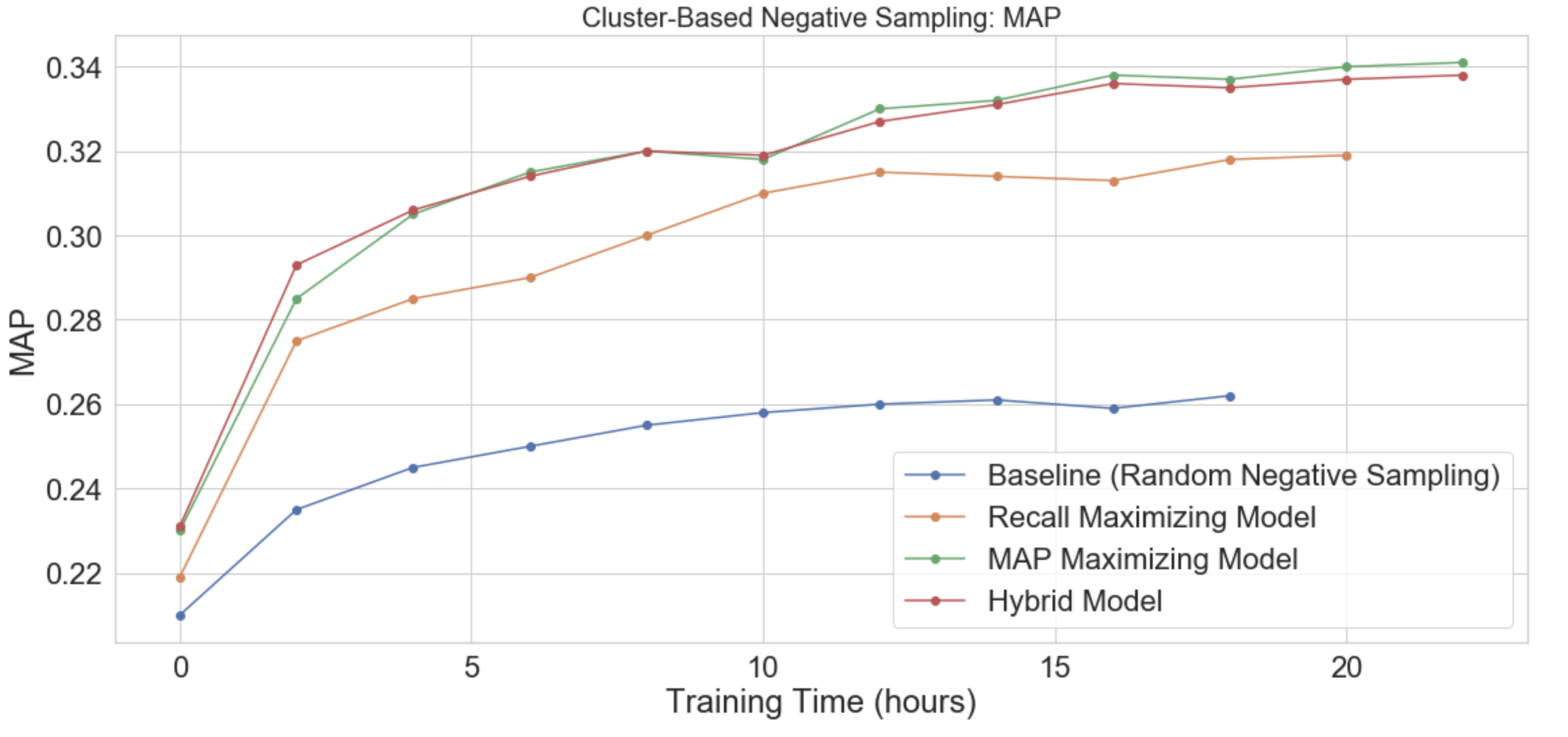
Since we are focused on ad hoc retrieval, we evaluate model performance on a hold-out validation test according to “Matching" Mean Average Precision (MAP) and “Matching" Recall as defined in (Nigam et al. 2019) where we first sample a set of 20,000 queries and evaluate the model’s ability to retrieve purchased products from a sub-corpus of 1 million products for those queries.
Tables 1 and 2 show the result of our parameter sweep on our evaluation set for our proposed negative sampling algorithm where each row corresponds to the number of graph clusters used while each column represents the number of nearby clusters probed for samples. We observe that we hit diminishing returns with too many clusters where we might split relevant items into different partitions and, consequently, sample related pairs as negatives. Similarly, we notice that increasing the number of probes improves model performance, which we hypothesize is due to sampling a greater diversity of negatives. However, increasing the number of probes comes at the cost of longer training times as we spend more computation within each training step sampling negatives.
| 8 | 16 | 32 | 64 | 128 | 256 | 512 | 1024 | ||
|---|---|---|---|---|---|---|---|---|---|
| 2048 | 0.317 | 0.318 | 0.319 | 0.314 | 0.312 | 0.304 | 0.295 | 0.285 | |
| 4096 | 0.323 | 0.326 | 0.327 | 0.321 | 0.320 | 0.312 | 0.306 | 0.293 | |
| 8192 | 0.328 | 0.330 | 0.339 | 0.331 | 0.332 | 0.321 | 0.312 | 0.302 | |
| 16384 | 0.329 | 0.333 | 0.338 | 0.336 | 0.338 | 0.332 | 0.319 | 0.309 | |
| 32768 | 0.323 | 0.332 | 0.338 | 0.337 | 0.334 | 0.339 | 0.328 | 0.310 | |
| 65536 | 0.306 | 0.322 | 0.332 | 0.334 | 0.335 | 0.341 | 0.331 | 0.307 | |
| 131072 | 0.286 | 0.302 | 0.327 | 0.331 | 0.338 | 0.337 | 0.329 | 0.298 |
| 8 | 16 | 32 | 64 | 128 | 256 | 512 | 1024 | ||
|---|---|---|---|---|---|---|---|---|---|
| 2048 | 0.761 | 0.775 | 0.780 | 0.778 | 0.784 | 0.780 | 0.772 | 0.761 | |
| 4096 | 0.754 | 0.767 | 0.777 | 0.781 | 0.784 | 0.783 | 0.782 | 0.770 | |
| 8192 | 0.739 | 0.757 | 0.775 | 0.782 | 0.790 | 0.787 | 0.789 | 0.778 | |
| 16384 | 0.724 | 0.747 | 0.762 | 0.773 | 0.786 | 0.788 | 0.790 | 0.782 | |
| 32768 | 0.703 | 0.723 | 0.746 | 0.757 | 0.772 | 0.787 | 0.786 | 0.778 | |
| 65536 | 0.672 | 0.697 | 0.715 | 0.743 | 0.763 | 0.775 | 0.782 | 0.771 | |
| 131072 | 0.635 | 0.661 | 0.696 | 0.720 | 0.743 | 0.760 | 0.768 | 0.754 |
Secondly, we can compare our best performing graph-based negative sampling models to our baseline with random negative sampling. Based on Tables 1 and 2, we select the model with the best performing MAP (65,536 clusters and 256 probes), the model with the best Recall (16,384 clusters and 512 probes) and a hybrid model that achieves strong performance on both metrics (16384 clusters, 128 probes). In Figures 5 and 6, we compare these models to a baseline which sampled negatives uniformly at random while keeping all other parameters fixed. In these plots, we compare the relative training times for each model by measuring metrics across hours of training time. Since the baseline involved no computation between each minibatch aside from uniform random sampling, each step of the baseline was approximately twice as fast as each step of the graph-based sampling models. However, these graph-based sampling models compensated for their added computation per step. They generalize better on the test set and achieve stronger performance on our validation metrics for every fixed unit of time past the start of training, allowing us to train a better model in less time than the baseline.

5.4. KNN Experiments
We next turn our attention to benchmarking the performance of our Partitioned Nearest Neighbor Search (PNNS) algorithmic framework for scaling KNN search on a billion-scale collection of vectors. We conducted grid searches on a smaller collection size of 3 million vectors to identify performant hyperparameter settings that achieved over 95% recall for each algorithm. Ultimately, we settled on the following parameter settings for our experiments:
- •
NGT: ESC=30, ESS=70 (ESC=10, ESS=20 with no partitioning)
- •
HNSW: EFC=700, EF=700, M=110
- •
IVF: NLIST=256, NUM PROBES=16
We note that we selected weaker hyper-parameter settings for NGT without partitioning because we observed that the algorithm would take an intractably long time (at least several months) to build the index otherwise. However, with PNNS partitioning, we were able to use more aggressive hyperparameters to achieve comparable latency and recall results to the other algorithms used in our experiment.
5.4.1. Index Build Time
One challenge with deploying approximate KNN algorithms at the billion scale is the fact that these approaches almost always involve a time-consuming step of converting input vectors into an index structure for searching. Many production search systems elect to rebuild their indexes at a regular cadence, such as every 24 hours. Although approximate approaches often dramatically reduce the search latency relative to a brute force search at marginal losses of recall, the index build time can possibly take multiple days, making daily rebuilds of the index infeasible. Through the PNNS graph partitioning approach, we can reduce this build time by building the indexes for each partition in parallel across multiple machines. Such a multi-machine index build is not currently supported by the libraries we experimented with.
Since we partition a bipartite graph of queries and products, the METIS algorithm enforces a balance between the sum of query and product nodes per cluster. Thus, we may still have a range in the number of products per cluster, as shown in Figure 7. As a result, we find that the overall index build time does not scale purely linearly with the number of machines since some of the partitions take longer to build than others because they contain more documents. This problem of efficiently building the indexes for each partition across some number of machines is an instance of the classic algorithmic task of assigning jobs to machines. For simplicity, we employ the well-known greedy algorithm of first sorting the jobs by their respective amounts of work and then iteratively assigning the most intensive remaining job to the machine currently with the lightest load. This approach guarantees an assignment of jobs where the maximum load across all machines is at most a constant factor of more than the optimal solution, as first shown in the classical paper of Graham 1969.

In Table 3, we report the index build time both for the standard KNN algorithms with no partitioning and with PNNS across a various number of machines. To conserve computational resources, we simulate running the PNNS index build over multiple machines by only running the jobs assigned to the machine with the maximum load, which will determine the overall index build time. From these results, we see that PNNS can reduce the cost of the overall index build time and, in some cases, make daily index builds feasible when such a cadence would not be possible without partitioning. We note that the times reported in Table 3 do not include the additional computation required for the graph partitioning. However, we can avoid re-running the partitioning step on a daily basis by assigning new documents to clusters via our classifier. Thus, in an amortized sense, the cost of graph partitioning becomes negligible compared to the cost of building the KNN indexes.
We also note that the savings in the build time from our partitioning scheme do come at the cost of increased computational resources as we construct the KNN indexes in parallel. However, since none of the algorithms/libraries we benchmark currently enable multi-machine index building, they cannot scale in the same manner with more compute resources. Thus, our method provides an avenue for indexing billion-scale embedding data for popular KNN search approaches within the constraints of a product build cadence, such as daily updates.
| NGT | HNSW | IVF | ||
| No Partitioning | >1000 | 87.2 | 9.28 | |
| PNNS (2 machines) | 77.03 | 33.37 | 2.12 | |
| PNNS (4 machines) | 38.35 | 18.15 | 1.03 | |
| PNNS (8 machines) | 23.5 | 12.13 | 0.533 | |
| PNNS (16 machines) | 21.07 | 11.42 | 0.483 |
5.4.2. Recall and Latency
In this section we focus on benchmarking the recall and latency of PNNS on our billion-scale collection size. As mentioned, we define recall as where is the set of results returned by an exact KNN search and is the items retrieved by the approximate algorithm. In our experiments, we focus on recall@100, namely the ability of the approximate algorithm to retrieve the top 100 results returned by an exact search. In Table 4, we report the average recall@100 across the 1000 queries we evaluated against. For latency, we measure the average time for each algorithm to return results across our 1000 benchmark queries.
In all of our PNNS experiments, we evaluate the algorithm’s recall and latency across varying number of probes. In addition, we fix the cumulative cluster probability hyperparameter to 0.99, meaning that we terminate our search early if the cumulative probability of the clusters we have searched within, as predicted by our cluster prediction classifier, exceeds this threshold.
| Number of Probes | NGT | HNSW | IVF | |
|---|---|---|---|---|
| 1 | 0.737 | 0.744 | 0.735 | |
| 2 | 0.838 | 0.846 | 0.833 | |
| 4 | 0.898 | 0.907 | 0.892 | |
| 8 | 0.934 | 0.943 | 0.928 | |
| 16 | 0.957 | 0.967 | 0.950 | |
| No Partitioning | 0.756 | 0.980 | 0.983 |
| Number of Probes | NGT | HNSW | IVF | |
|---|---|---|---|---|
| 1 | 38.03 | 71.61 | 199.82 | |
| 2 | 53.90 | 113.09 | 277.93 | |
| 4 | 89.85 | 183.89 | 526.60 | |
| 8 | 151.09 | 300.39 | 812.89 | |
| 16 | 289.12 | 453.69 | 1265.90 | |
| No Partitioning | 90.0 | 36.54 | 30313.07 |
From Tables 4 and 5, we see that PNNS, for a larger fraction of probes, can achieve slightly reduced recall numbers compared to the standard HNSW algorithm without partitioning, but at the cost of increased latency. In practice, this tradeoff might still be favorable given the potential for a considerably decreased index build time as shown in Table 3. In addition, we find that PNNS can enable us to use more performant hyperparameter settings for NGT since the index build time becomes tractable. As a result, PNNS can provide a path for deploying NGT at the billion scale in practice and provides feasible latency and recall results across a variety of probes. The IVF algorithm has a significantly smaller index build time than the other methods we benchmarked, but comes at the cost of a much larger latency (though still orders-of-magnitude faster than an exact search). For IVF, we found that PNNS produced relatively marginal savings in index build time, but was able to reduce the search latency by an order of magnitude with a small reduction in recall.
In summary, we found that PNNS can serve as a general algorithmic framework to run the popular HNSW and NGT approximate algorithms at the billion scale in practical settings by making daily index builds feasible. In the case of IVF, PNNS also reduced the search latency considerably. When assessing the tradeoffs between PNNS and the baselines techniques, we note that building the search index within 24 hours to facilitate daily updates may be an essential requirement for real production systems, in which case the ability of PNNS to parallelize the index build process may be essential at this scale despite the loss of some recall and a potential increase in latency. Furthermore, we note that each of the billion-scale KNN search indexes with no partitioning that we experimented with yielded a memory footprint of over 1 terabyte. While we were able to accommodate these large indexes in our experiments thanks to our use of an AWS x1 instance, we note that many practitioners might be looking for ways to deploy cheaper instances in production settings. The efficient partitioning strategy behind PNNS also provides a path for enabling distributed nearest neighbor search where we can store the indexes for each partition, which will have smaller memory footprints than the full index, over multiple machines and thereby sidestep this memory bottleneck. In this sense, PNNS, while possibly producing some regression in latency or recall when compared to its unpartitioned counterpart algorithm, may be an essential step in deploying nearest neighbor search at the billion scale within the practical constraints of real systems.
5.4.3. Deployment
We successfully deployed PNNS-based search for several weeks in an online A/B test on a large e-commerce website to augment the traditional inverted index-based keyword matches with products retrieved by our neural embedding model. We validated that PNNS was able to meet the constraints of the search system while improving several business metrics. These results also validate that learned index structures can be integrated into established production systems and meet strict engineering requirements where data-independent algorithms fall short.
6. Conclusion and Future Work
In this paper, we address the problem of performing training and inference for dyadic embedding models at the billion scale, focusing on the practical application of semantic product search. To our knowledge, our work is the first to present solutions for deploying embedding-based retrieval at this scale under the constraints of realistic industrial systems. We demonstrated that the same underlying principle of leveraging the structure of real-world data can tackle both of these problems. By modeling dyadic data as a bipartite graph and utilizing balanced graph partitioning algorithms, we showed both improved model performance and reduced convergence time during training through efficient hard negative sampling. In addition, we presented a technique, based on graph clustering and a learned classifier, for scaling popular KNN algorithms in terms of either search time (in the case of IVF) or in sharply reducing the index build time (in the case of NGT and HNSW) with minimal impact on recall. Unlike similar graph partitioning approaches for KNN search in the literature, our technique leverages a graph already constructed from the underlying dyadic data and thereby eliminates the computationally prohibitive step of constructing a KNN graph at the billion scale. For future work on the negative sampling side, we can investigate curriculum learning strategies for our graph-based negative sampling approach where we tighten the window of adjacent cluster to sample from over the course of training. On the inference side, as mentioned in (Dong et al. 2020), we can consider investigating methods for learning the graph partitioning and the cluster prediction model in an end-to-end fashion where one optimization problem informs the other. Finally, we note that our proposed techniques are general in nature and can be applied to numerous problem domains that fit the dyadic data paradigm, and we hope to extend our ideas to other applications beyond product search.
References
- (1)
- Andoni and Indyk (2006) Alexandr Andoni and Piotr Indyk. 2006. Near-optimal hashing algorithms for approximate nearest neighbor in high dimensions. In 2006 47th annual IEEE symposium on foundations of computer science (FOCS’06). IEEE, 459–468.
- Andreev and Racke (2006) Konstantin Andreev and Harald Racke. 2006. Balanced graph partitioning. Theory of Computing Systems 39, 6 (2006), 929–939.
- Bentley (1975) Jon Louis Bentley. 1975. Multidimensional binary search trees used for associative searching. Commun. ACM 18, 9 (1975), 509–517.
- Bernhardsson (2017) E Bernhardsson. 2017. ANNOY: Approximate nearest neighbors in C++/Python optimized for memory usage and loading/saving to disk. GitHub https://github. com/spotify/annoy (2017).
- Boytsov and Naidan (2013) Leonid Boytsov and Bilegsaikhan Naidan. 2013. Engineering Efficient and Effective Non-metric Space Library. In Similarity Search and Applications - 6th International Conference, SISAP 2013, A Coruña, Spain, October 2-4, 2013, Proceedings (Lecture Notes in Computer Science, Vol. 8199), Nieves R. Brisaboa, Oscar Pedreira, and Pavel Zezula (Eds.). Springer, 280–293. https://doi.org/10.1007/978-3-642-41062-8_28
- Dong et al. (2020) Yihe Dong, Piotr Indyk, Ilya Razenshteyn, and Tal Wagner. 2020. Learning Space Partitions for Nearest Neighbor Search. (2020).
- Fu et al. (2019) Cong Fu, Chao Xiang, Changxu Wang, and Deng Cai. 2019. Fast Approximate Nearest Neighbor Search With The Navigating Spreading-out Graphs. PVLDB 12, 5 (2019), 461 – 474. https://doi.org/10.14778/3303753.3303754
- Gao et al. (2015) Jinyang Gao, HV Jagadish, and Beng Chin Ooi. 2015. Active sampler: Light-weight accelerator for complex data analytics at scale. arXiv preprint arXiv:1512.03880 (2015).
- Gionis et al. (1999) Aristides Gionis, Piotr Indyk, Rajeev Motwani, et al. 1999. Similarity search in high dimensions via hashing. In Vldb, Vol. 99. 518–529.
- Graham (1969) R. L. Graham. 1969. Bounds on Multiprocessing Timing Anomalies. SIAM JOURNAL ON APPLIED MATHEMATICS 17, 2 (1969), 416–429.
- Guo et al. (2018) Guibing Guo, Songlin Zhai, Fajie Yuan, Yuan Liu, and Xingwei Wang. 2018. Vse-ens: Visual-semantic embeddings with efficient negative sampling. In Thirty-Second AAAI Conference on Artificial Intelligence.
- Guo et al. (2016) Jiafeng Guo, Yixing Fan, Qingyao Ai, and W Bruce Croft. 2016. A deep relevance matching model for ad-hoc retrieval. In Proceedings of the 25th ACM International on Conference on Information and Knowledge Management. ACM, 55–64.
- Hofmann et al. (1999) Thomas Hofmann, Jan Puzicha, and Michael I Jordan. 1999. Learning from dyadic data. In Advances in neural information processing systems. 466–472.
- Hu et al. (2014) Baotian Hu, Zhengdong Lu, Hang Li, and Qingcai Chen. 2014. Convolutional Neural Network Architectures for Matching Natural Language Sentences. In Proceedings of the 27th International Conference on Neural Information Processing Systems - Volume 2 (Montreal, Canada) (NIPS’14). MIT Press, Cambridge, MA, USA, 2042–2050. http://dl.acm.org/citation.cfm?id=2969033.2969055
- Huang et al. (2013) Po-Sen Huang, Xiaodong He, Jianfeng Gao, Li Deng, Alex Acero, and Larry Heck. 2013. Learning deep structured semantic models for web search using clickthrough data. In Proceedings of the 22nd ACM international conference on Conference on information & knowledge management. ACM, 2333–2338.
- Hui et al. (2017a) Kai Hui, Andrew Yates, Klaus Berberich, and Gerard de Melo. 2017a. Pacrr: A position-aware neural ir model for relevance matching. arXiv preprint arXiv:1704.03940 (2017).
- Hui et al. (2017b) Kai Hui, Andrew Yates, Klaus Berberich, and Gerard de Melo. 2017b. Re-pacrr: A context and density-aware neural information retrieval model. arXiv preprint arXiv:1706.10192 (2017).
- Hui et al. (2018) Kai Hui, Andrew Yates, Klaus Berberich, and Gerard de Melo. 2018. Co-pacrr: A context-aware neural ir model for ad-hoc retrieval. In Proceedings of the Eleventh ACM International Conference on Web Search and Data Mining. ACM, 279–287.
- Indyk and Motwani (1998) Piotr Indyk and Rajeev Motwani. 1998. Approximate nearest neighbors: towards removing the curse of dimensionality. In Proceedings of the thirtieth annual ACM symposium on Theory of computing. ACM, 604–613.
- Iwasaki (2015) Masajiro Iwasaki. 2015. Ngt: Neighborhood graph and tree for indexing.
- Jegou et al. (2010) Herve Jegou, Matthijs Douze, and Cordelia Schmid. 2010. Product quantization for nearest neighbor search. IEEE transactions on pattern analysis and machine intelligence 33, 1 (2010), 117–128.
- Johnson et al. (2017) Jeff Johnson, Matthijs Douze, and Hervé Jégou. 2017. Billion-scale similarity search with GPUs. arXiv preprint arXiv:1702.08734 (2017).
- Johnson and Guestrin (2018) Tyler B Johnson and Carlos Guestrin. 2018. Training deep models faster with robust, approximate importance sampling. In Advances in Neural Information Processing Systems. 7265–7275.
- Karypis and Kumar (1998) George Karypis and Vipin Kumar. 1998. A fast and high quality multilevel scheme for partitioning irregular graphs. SIAM Journal on scientific Computing 20, 1 (1998), 359–392.
- Kingma and Ba (2014) Diederik P Kingma and Jimmy Ba. 2014. Adam: A method for stochastic optimization. arXiv preprint arXiv:1412.6980 (2014).
- Kraska et al. (2018) Tim Kraska, Alex Beutel, Ed H. Chi, Jeffrey Dean, and Neoklis Polyzotis. 2018. The Case for Learned Index Structures. In Proceedings of the 2018 International Conference on Management of Data (Houston, TX, USA) (SIGMOD ’18). ACM, New York, NY, USA, 489–504.
- Malkov and Yashunin (2018) Yury A Malkov and Dmitry A Yashunin. 2018. Efficient and robust approximate nearest neighbor search using hierarchical navigable small world graphs. IEEE transactions on pattern analysis and machine intelligence (2018).
- Mitra and Craswell (2017) Bhaskar Mitra and Nick Craswell. 2017. Neural models for information retrieval. arXiv preprint arXiv:1705.01509 (2017).
- Mitra et al. (2017) Bhaskar Mitra, Fernando Diaz, and Nick Craswell. 2017. Learning to match using local and distributed representations of text for web search. In Proceedings of the 26th International Conference on World Wide Web. International World Wide Web Conferences Steering Committee, 1291–1299.
- Nigam et al. (2019) Priyanka Nigam, Yiwei Song, Vijai Mohan, Vihan Lakshman, Weitian Allen Ding, Ankit Shingavi, Choon Hui Teo, Hao Gu, and Bing Yin. 2019. Semantic Product Search. In Proceedings of the 25th ACM SIGKDD International Conference on Knowledge Discovery & Data Mining. ACM, 2876–2885.
- Palangi et al. (2016) Hamid Palangi, Li Deng, Yelong Shen, Jianfeng Gao, Xiaodong He, Jianshu Chen, Xinying Song, and Rabab Ward. 2016. Deep sentence embedding using long short-term memory networks: Analysis and application to information retrieval. IEEE/ACM Transactions on Audio, Speech and Language Processing (TASLP) 24, 4 (2016), 694–707.
- Pang et al. (2016) Liang Pang, Yanyan Lan, Jiafeng Guo, Jun Xu, Shengxian Wan, and Xueqi Cheng. 2016. Text Matching as Image Recognition.. In AAAI. 2793–2799.
- Pellegrini and Roman (1996) François Pellegrini and Jean Roman. 1996. Scotch: A software package for static mapping by dual recursive bipartitioning of process and architecture graphs. In International Conference on High-Performance Computing and Networking. Springer, 493–498.
- Sablayrolles et al. (2018) Alexandre Sablayrolles, Matthijs Douze, Cordelia Schmid, and Hervé Jégou. 2018. Spreading vectors for similarity search. arXiv preprint arXiv:1806.03198 (2018).
- Sanders and Schulz (2013) Peter Sanders and Christian Schulz. 2013. Think Locally, Act Globally: Highly Balanced Graph Partitioning. In Proceedings of the 12th International Symposium on Experimental Algorithms (SEA’13) (LNCS, Vol. 7933). Springer, 164–175.
- Shen et al. (2014) Yelong Shen, Xiaodong He, Jianfeng Gao, Li Deng, and Grégoire Mesnil. 2014. A latent semantic model with convolutional-pooling structure for information retrieval. In Proceedings of the 23rd ACM International Conference on Conference on Information and Knowledge Management. ACM, 101–110.
- Sivic and Zisserman (2003) Josef Sivic and Andrew Zisserman. 2003. Video Google: A text retrieval approach to object matching in videos. In null. IEEE, 1470.
- Slota et al. (2014) George M Slota, Kamesh Madduri, and Sivasankaran Rajamanickam. 2014. PuLP: Scalable multi-objective multi-constraint partitioning for small-world networks. In 2014 IEEE International Conference on Big Data (Big Data). IEEE, 481–490.
- Wan et al. (2016) Shengxian Wan, Yanyan Lan, Jun Xu, Jiafeng Guo, Liang Pang, and Xueqi Cheng. 2016. Match-srnn: Modeling the recursive matching structure with spatial rnn. arXiv preprint arXiv:1604.04378 (2016).
- Ying et al. (2018) Rex Ying, Ruining He, Kaifeng Chen, Pong Eksombatchai, William L Hamilton, and Jure Leskovec. 2018. Graph convolutional neural networks for web-scale recommender systems. In Proceedings of the 24th ACM SIGKDD International Conference on Knowledge Discovery & Data Mining. ACM, 974–983.