Data Harmonization Via Regularized Nonparametric Mixing Distribution Estimation

Steven Wilkins-Reeves Yen-Chi Chenabel=e2 mark]yenchic@uw.edu Kwun Chuen Gary Chanabel=e3 mark]kcgchan@uw.edu Steven Wilkins-Reeves Yen-Chi Chenabel=e2 mark]yenchic@uw.edu Kwun Chuen Gary Chanabel=e3 mark]kcgchan@uw.edu

Supplement to: Data Harmonization Via Regularized Nonparametric Mixing Distribution Estimation

Data harmonization is the process by which an equivalence is developed between two variables measuring a common trait. Our problem is motivated by dementia research in which multiple tests are used in practice to measure the same underlying cognitive ability such as language or memory. We connect this statistical problem to mixing distribution estimation. We introduce and study a non-parametric latent trait model, develop a method which enforces uniqueness of the regularized maximum likelihood estimator, show how a nonparametric EM algorithm will converge weakly to its maximizer, and additionally propose a faster algorithm for learning a discretized approximation of the latent distribution. Furthermore, we develop methods to assess goodness of fit for the mixing likelihood which is an area neglected in most mixing distribution estimation problems. We apply our method to the National Alzheimer’s Coordination Center Uniform Data Set and show that we can use our method to convert between score measurements and account for the measurement error. We show that this method outperforms standard techniques commonly used in dementia research.

, and

^??Department of Statistics, University of Washington, ??; ??

^??Department of Biotatistics, University of Washington, ??

1 Introduction

Data harmonization is the process by which measurements from different sources and by different methods are combined into a single dataset for further analysis. It often involves converting scores between two different measurements of the same trait, which is the main focus of this paper. For example, in neuropsychological testing for Alzheimer’s Disease, collections of tests known as batteries are used to measure a variety of cognitive traits such as attention, language, episodic memory, visual-spatial ability etc. Different studies, or even in the same study, may use different validated instruments to measure each trait. As an increasing number of data sets are becoming available for public use, data harmonization efforts are common in order to create harmonized variables in the combined data set.

This study is motivated by the different cognitive measurements in the Neuropsychological Test Battery of the National Alzheimer’s Coordinating Center (NACC) Uniform Data Set (UDS). The NACC UDS has the largest number of participants for studying the progression to mild cognitive impairment and dementia in the United States (Weintraub et al. 2009; Besser et al. 2018). The batteries used for neuropsychological assessment of an individual change over time. In 2015, the third version of the Uniform Data Set developed a non-proprietary neuropsychological battery which may be used to standardise results across individuals going forward, while prior to that time, a different set of proprietary neuropsychological battery was given. Additionally for comparison across tests, a small group of cognitively normal individuals received both the old score battery and new battery in a crosswalk study (Monsell et al. 2016) which will serve as a validation sample of various harmonization methods.

In general, data harmonization requires two main steps. The first of which is to determine whether two variables $Y\in\{0,1,2,\dots,N_{Y}\}$ and $Z\in\{0,1,2,\dots,N_{Z}\}$ measure the same trait. That is, whether their distributions can be commonly represented by a single latent variable $\gamma$ . This may either require expert knowledge or studies of individuals completing both tests. In our case, the change in battery and their correspondence in measuring cognitive domains were guided by the Clinical Task Force (CTF), a group formed by the National Institutes of Aging to develop standardized methods for collecting longitudinal data that would encourage and support collaboration across the Alzheimer’s Disease Research Centers. The second step is to propose a joint model of the scores, frequently using a latent variable representation (Griffith et al. 2013; van den Heuvel et al. 2020).

These methods, however, tend to mostly rely on parametric assumptions (Griffith et al. 2013). Additionally, rather than focusing on inference associated how the difficiculty of tests vary with covariates, we are interested in predicting the outcome of a test $Z$ given an individual’s score on test $Y$ .

In this paper, we consider a non-parametric approach to latent variable modelling for the purpose of data harmonization. We connect this approach to mixing distribution estimation, for which there is a rich history. One of the earliest versions of the problem arose from educational testing as estimating a population of parameters for individuals taking a test where scores for each individual are assumed follow a binomial distribution with parameters $N,p_{i}$ (Lord 1965; Lord 1969), where $p_{i}$ follows a certain distribution. The binomial case is a particularly well studied application of mixing distribution estimation (Lindsay 1983a; Wood 1999; Tian, Kong and Valiant 2017; Vinayak et al. 2019). Estimation of a mixing distribution in general has numerous other applications such as in positron emission tomography (Vardi, Shepp and Kaufman 1985; Silverman et al. 1990a), portfolio optimization (Cover 1984) and ecology (Bell, Lechowicz and Waterway 2000). In cases where $Y$ is continuous, de-convolution kernels are a common approach (Leonard and Carroll 1990; Basulto-Elias et al. 2021) as this becomes a more standard measurement error problem. Recently there has also been an operator theoretic study of mixing distribution estimation (Van Dermeulen and Scott 2019).

The nonparametric EM algorithm (Laird 1978) is a classical approach to compute the nonparametric maximum likelihood estimator (NPMLE) (Kiefer and Wolfowitz 1956). An assumption was made by Laird initially that the maximum likelihood estimator should be a discrete distribution. This problem was formalized by Lindsay 1983b who proved that under some very mild conditions there always exists a discrete maximum likelihood estimator of the mixing distribution, even if the true mixing distribution is continuous. This phenomena is partly reconciled by the non-identifiability of the maximum likelihood estimate for the mixing distribution. However, when the goal is data harmonization, a discrete estimated mixture distribution may be undesirable, since in data harmonization, it is often assumed that a continuous latent map exists between latent variables and a discrete latent distribution would violate this assumption (van den Heuvel et al. 2020). We will address this problem by a regularization approach.

The remainder of the paper will outline our statistical approach to this data harmonization problem. First we introduce a graphical representation for our problem. We focus on non-parametric estimation of the mixing distributions, as well as introduce a regularized estimator. We further focus on the aspects of picking the conditional distribution (measurement error) assumption required for modelling, as well as testing the feasibility of the assumption.

2 Methods

Consider a set of i.i.d. random variables $(X_{i},Y_{i},Z_{i},A_{i})$ , where $X_{i}\in\mathbb{R}^{d}$ is a set of covariates and $Y_{i}\in\{0,\dots,N_{Y}\}$ is the old score and $Z_{i}\in\{0,\dots,N_{Z}\}$ is the new scores. We drop the subscript on $N$ if it is clear from the context. We focus on discrete test scores as the neuropsychological tests considered in the application are all discrete. Lastly, $A_{i}\in\{0,1\}$ is an indicator determining which score is observed. In this setting only one score is observed for each individual, denote $A_{i}=0$ if score $Y_{i}$ is observed and $A_{i}=1$ if score $Z_{i}$ is observed. Our motivation comes from heterogeneous measurements of a common trait. In our application, we think of this as two test scores measuring the same cognitive area, such as language or memory. We next introduce our fundamental assumption of data harmonization.

Definition 2.1 (Harmonizable Variables).

Two discrete variables $Y$ and $Z$ are harmonizable if (a) they are independent of all other variables, conditional on a continuous latent variables $\gamma,\zeta\in[0,1]$ respectively, and (b) conditioned on covariates $X$ , there is an invertible and increasing mapping between the two latent variables $\phi_{\gamma\to\zeta}$ such that for all $X$

\zeta=\phi_{\gamma\to\zeta}\left(\gamma|X\right).

(1)

Theorem 2.2.

If $Y$ and $Z$ are harmonizable variables with latent variables $\gamma,\zeta$ , the mappings $\phi_{\gamma\to\zeta}(\cdot|x)$ and $\phi_{\zeta\to\gamma}(\cdot|x)$ uniquely exist and can be defined below:

	$\displaystyle\phi_{\gamma\to\zeta}(q\|x)$	$\displaystyle=G^{-1}\left(F(q\|x)\|x\right)$		(2)
	$\displaystyle\phi_{\zeta\to\gamma}(q\|x)$	$\displaystyle=F^{-1}\left(G(q\|x)\|x\right)=\phi^{-1}_{\gamma\to\zeta}(q\|x)$		(3)

where $F(\cdot|x)$ and $G(\cdot|x)$ are the conditional CDF’s of $\gamma$ and $\zeta$ respectively

We assume $\gamma$ and $\zeta$ must have continuous conditional CDF’s then:

	$\displaystyle G(q\|x)$	$\displaystyle=P(\zeta\leq q\|x)$
		$\displaystyle=P(\phi_{\gamma\to\zeta}(\gamma\|x)\leq q\|x)$
		$\displaystyle=P(\gamma\leq\phi^{-1}_{\gamma\to\zeta}(q\|x)\|x)$
		$\displaystyle=F(\phi^{-1}_{\gamma\to\zeta}(q\|x)\|x)$
	$\displaystyle\implies\phi^{-1}_{\gamma\to\zeta}(q\|x)$	$\displaystyle=F^{-1}(G(q\|x)\|x)\text{ and }\phi_{\gamma\to\zeta}(q\|x)=G^{-1}(F(q\|x)\|x)$

∎

If two random variables are harmonizable, they must be measuring the same trait. This assumption is similar to that of rank preserving models though we do not assume an constant additive effect (Robins and Tsiatis 1991; White et al. 1997; White et al. 1999). A simple generative model for a pair of harmonizable variables is the following hierarchical model:

$\displaystyle\Omega_{i}$	$\displaystyle\sim U(0,1),$	$\displaystyle X_{i}$	$\displaystyle\sim P_{X}$	(4)
$\displaystyle\gamma_{i}$	$\displaystyle=F^{-1}(\Omega_{i}\|X_{i}),$	$\displaystyle\zeta_{i}$	$\displaystyle=G^{-1}(\Omega_{i}\|X_{i})$
$\displaystyle Y_{i}\|\gamma_{i}$	$\displaystyle\sim P_{A_{Y}}(\cdot\|\gamma_{i}),$	$\displaystyle Z_{i}$	$\displaystyle\|\zeta_{i}\sim P_{A_{Z}}(\cdot\|\zeta_{i})$
$\displaystyle A$	$\displaystyle\perp\!\!\!\perp(\Omega,Y,Z)\|X$

where $U(0,1)$ represents a uniform random variable, $P_{X}$ represents the distribution of the covariates, $F^{-1}(\cdot|x),G^{-1}(\cdot|x)$ represent the inverse of the conditional cdfs of $\gamma$ and $\zeta$ respectively and $P_{A_{Y}}$ (or $P_{A_{Z}}$ ) represents the corresponding distribution of the observed score, given the latent trait (i.e. the measurement error). We summarize this hierarchical model using Figure 1. This is not a conventional graphical model, but we use the graph to summarize the generative assumption of our model. The square variables denote that these variables are deterministic functions of their parent variables.

Fig 1: Score Generation Model. Deterministic relationships between latent variables shown in blue. Deterministic variables dependent on upstream variables shown with squares.

The generative model in equation (4) can be interpreted as follows. $\Omega$ is the relative quantile of an individual’s cognitive ability in the population. Thus, $\Omega$ together with the covariate $X$ determines the latent traits $\gamma,\zeta$ of the two tests. The observed scores $Y$ and $Z$ are the measured version of the latent traits, so they are completely determined by $\gamma$ and $\zeta$ , respectively. The conditional independence $A\perp\!\!\!\perp(\Omega,Y,Z)|X$ is motivated by the fact that the score conversion in the NACC data occurs at 2015, which is not relevant to any individual’s ability (but it may be relevant to the year of visit/age, which is part of the covariate $X$ ),

Although we only observe either $(X_{i},Y_{i},A_{i}=0)$ or $(X_{i},Z_{i},A_{i}=1)$ , the generative model in equation (4) implies that the observed data is determined by $p(y|\gamma),p(z|\zeta),p(\gamma|x),p(\zeta|x)$ , $p(a|x)$ and $p(x)$ . For the purpose of data harmonization, we do not need to model $p(a|x)$ or $p(x)$ , so we will focus on modeling the first four distributions. The first two distributions $p(y|\gamma),p(z|\zeta)$ are the measurement Assumptions, so we denote them as $p_{A}(y|\gamma),p_{A}(z|\zeta)$ . The two distributions $p(\gamma|x),p(\zeta|x)$ are the latent trait Models, so we denote them as $p_{M}(\gamma|x),p_{M}(\zeta|x)$ . In what follows, we describe how we model $p_{A}$ and $p_{M}$ . To simplify the notations, we focus on $p_{A}(y|\gamma)$ and $p_{M}(\gamma|x)$ ; the case of $p_{A}(z|\zeta)$ and $p_{M}(\zeta|x)$ can be modeled in a similar manner.

Remark. We can immediately draw a comparison from this representation to the Skorohod notation of a random variable which are introduced in quantile regression models (not to be confused with the Skorohod representation theorem) (Chernozhukov and Hansen 2006; Kato 2012).

Remark. We contrast this with the approach of (van den Heuvel et al. 2020), in which they assume that the distribution of $Y|\gamma$ may not be independent of $X$ , however the mapping between latent variables $\phi_{\gamma\to\zeta}$ is independent of $X$ . Our measurement assumption is similar to (Meredith 1993) in which $p(y|\gamma,x)=p(y|\gamma)$ and similarly for $Z$ .

2.1 Measurement Assumption Model

A conventional approach for modeling $p_{A}$ is the binomial model (Lindsay 1983a; Wood 1999; Tian, Kong and Valiant 2017; Vinayak et al. 2019), for measurements that are sum scores of a fixed number of binary question items. However, this may be a restrictive assumption as it inherently depends on equal difficulties for each test question with independent responses. If we had access to all the question items, it would be possible to learn a conditional model with the difficulties for each question using a Rasch model (Rasch 1966; Lindsay, Clogg and Grego 1991) or a more elaborate IRT model. In the NACC UDS application, the individual binary question items are not available. The measurement assumption model can be selected by a domain expert, but additionally we can also test for its feasibility as we present in Section 3.1 as well as present a method for selecting this model from the data in Section 3.2.

In this paper, we propose a flexible method to construct a measurement assumption by measurement kernel (functions). Specifically, we model the measurement assumption as

p_{A}(y|\gamma)\propto K\left(\frac{y-N\gamma}{h}\right),

(5)

where $K$ is the measurement kernel and $h>0$ is the smoothing bandwidth. This model enables great flexibility in terms of the shape of the error distribution, controlled by $K$ and the spread of the distribution, controlled by $h$ . We also denote $Y|\gamma\sim MKM(K,h,\gamma)$ if the conditional distribution is defined by the model above. The kernel function defines the relative probability of the conditional distribution $Y|\gamma$ with assigning higher probability for $y$ near $N\gamma$ . $K$ defines the decay of the relative probability as $y$ is further from $N\gamma$

2.2 Latent Trait Models

2.2.1 Non-Parametric Model

In many applications, parametric models for a latent model may not be particularly realistic. As a result, we would like to relax this assumption and consider a non-parametric method. We propose a model based on the non-parametric EM algorithm (Laird 1978). To simplify the derivation, we omit the covariate $X$ . We illustrate how we can incorporate covariates in Section 2.2.3. Estimating the latent model $p_{M}(\gamma)$ now clearly becomes a mixing distribution problem with log-likelihood:

\ell_{n}[P_{M}]=\frac{1}{n}\sum_{i=1}^{n}\log\left(\int p_{A}(y_{i}|\gamma)p_{M}(\gamma)d\gamma\right)\quad P_{M}\in\mathcal{P}_{[0,1]}

(6)

where we differentiate the parametric likelihood $\ell_{n}(\theta)$ from the functional likelihood $\ell_{n}[P_{M}]$ , with $\mathcal{P}_{[0,1]}$ denotes the space of all probability measures over $[0,1]$ . We also highlight that $P_{M}$ refers to the measure which has a corresponding generalized density function $p_{M}$ for which we may allow point masses. This problem involves solving the NPMLE (Kiefer and Wolfowitz 1956) and was the original inspiration for the nonparametric EM algorithm (NPEM, also known as the functional EM) (Laird 1978).

With a basic rearrangement, we can rewrite equation (6), the mixture likelihood, to the following:

\ell_{n}[P_{M}]=\sum_{y=0}^{N}\widehat{p}(y)\log\left(\int p_{A}(y_{i}|\gamma)p_{M}(\gamma)d\gamma\right)

(7)

where $\widehat{p}(y)$ is the empirical distribution of $y$

\widehat{p}(y)=\frac{1}{n}\sum_{i=1}^{n}I(Y_{i}=y).

(8)

This leads us to the standard nonparametric EM algorithm (Laird 1978)

p_{M}^{(j+1)}(\gamma)=\mbox{$\mathbb{E}$}_{\widehat{p}(y)}[p_{M}^{(j)}(\gamma|y)]=\sum_{y=0}^{N}\frac{p_{A}(y|\gamma)\widehat{p}(y)p^{(j)}(\gamma)}{p_{MA}^{(j)}(y)}

(9)

where $p_{MA}^{(j)}(y)=\int p_{A}(y|\gamma)p_{M}^{(j)}(\gamma)d\gamma$ .

Remark. (Lindsay 1983b) studied the nonparametric EM in depth and proved that if $Y$ has a support size of $N+1$ , then there will always exists a discrete NPMLE with at most $N+1$ masses, even under a true model where $p_{0}(\gamma)$ is continuous. This phenomena is explained by the non-identifiability of this model in general, which we will address further in section 2.2.2. Approaches to ensure smoothness have also been developed for the latent density estimation such as early stopping of an EM algorithm (Chae, Martin and Walker 2017), imposing a roughness penalty on the density likelihood (Liu, Levine and Zhu 2009) or using a kernel density smoother between iterations of an EM algorithm (Silverman et al. 1990b). The early stopping is not ideal as we are intentionally not fully maximizing the likelihood. The kernel density method of Silverman et al. 1990b also has problems of how to choose the smoother bandwith, as well as losing the non-decreasing property of the EM algorithm. The roughness penalized method of Liu, Levine and Zhu 2009 is challenging to compute as they introduce an EM algorithm which requires solving an ODE at each iteration.

Under the conditions of Chung and Lindsay 2015, the update in equation (9) leads to an improved estimator in the sense that the implied marginal distribution of $Y$ is closer to the empirical distribution in relative entropy. We next introduce a theorem that under a list of sharpness conditions on $p_{A}$ which are listed in supplement A, we will have linear convergence.

Theorem 2.3.

Under the assumptions listed in the supplementary material part A, the NPEM algorithm will converge linearly (in the 1-norm) with rate $\rho\in[0,1)$

||{p_{MA}^{(t+1)}(y)-\widehat{p}(y)}||_{1}\leq\rho||{p_{MA}^{(t)}(y)-\widehat{p}(y)}||_{1}.

Though the assumptions required for linear convergence are rather strict, they reflect a broader trend seen empirically where a sharper measurement assumption model $p_{A}$ tends to converge faster with the nonparametric EM algorithm. In general, this algorithm must be approximated since we do not have an exact evaluation of the integral to compute $p^{(j+1)}_{M}(\gamma)$ . We illustrate an approximation of this method in the supplementary material part A.

The nonparametric likelihood in equation (9) suffers from a non-identifiability problem as the likelihood functional $\ell_{n}[P_{M}]$ is only concave in $P_{M}$ , not strictly concave. Namely, there might be multiple distributions which maximize $\ell_{n}[P_{M}]$ . Due to the non-identifiability of a maximizer, the convergence properties of the nonparametric EM algorithm are far less studied than in the parametric case. As far as we are aware, Chung and Lindsay 2015 is the only work that proved the convergence of nonparametric EM in terms of likelihood values but it did not derive the rate as Theorem C.1.

Though the mixing distribution $P_{M}$ is not identifiable, we still may find that the imposed distribution on the marginal $p_{MA}$ will converge linearly to $\widehat{p}$ , the empirical distribution under the regularity conditions outlined in the supplement.

2.2.2 Regularized Nonparametric Latent Trait

To deal with the non-identifiability issue, we introduce a regularized NPEM algorithm leading to a unique maximizer. Let $P_{U}$ be the measure of a uniform random variable over [0,1]. We introduce a regularization term via the KL-divergence from the uniform distribution, i.e., $\mathcal{D}(P_{U}||P_{M})$ .

We define the regularized likelihood as

\displaystyle\ell_{n,\mu}[P_{M}]

\displaystyle=\ell_{n}[P_{M}]-\mu\mathcal{D}(P_{U}||P_{M}).

Due to the strict convexity of $\mathcal{D}(P_{U}||P_{M})$ in each parameter, the regularized objective has a unique maximizer whenever $\mu>0$ . One reason of regularizing to a uniform density is due to its reasonable choice as an uninformative latent distribution much like the choice of regularizing coefficients to $0$ in the LASSO (Tibshirani 1996). Additionally, since a discrete latent distribution $p_{M}$ will have infinite KL-divergence from the uniform $\mathcal{D}(P_{U}||P_{M})$ , regularizing toward a uniform distribution will smooth the estimate depending on the parameter $\mu$ . Moreover, this choice of regularization penalty leads to computational convenience. We outline two methods which can be used to compute the regularized nonparametric MLE (RNPMLE).

Optimization Algorithm 1 : Regularized NPEM algorithm. The NPEM algorithm only requires a minor change for the likelihood which includes a regularization term, and this NPEM algorithm amounts to estimating a mixture between the standard EM step and with a uniform distribution.

We derive the form of the update much like the original EM algorithm:

	$\displaystyle\ell_{n,\mu}[P_{M}]$	$\displaystyle=\sum_{y=0}^{N}\widehat{p}(y)\log\left(\int p_{A}(y\|\gamma)p_{M}(\gamma)d\gamma\right)-\mu\mathcal{D}(P_{U}\|\|P_{M})$
		$\displaystyle=\sum_{y=0}^{N}\widehat{p}(y)\log\left(p_{MA}(y)\right)-\mu\mathcal{D}(P_{U}\|\|P_{M})$
		$\displaystyle=\sum_{y=0}^{N}\widehat{p}(y)\left(\log\left(p_{MA}(y,\gamma)\right)-\log\left(p_{MA}(\gamma\|y)\right)\right)-\mu\mathcal{D}(P_{U}\|\|P_{M})$
		$\displaystyle=\sum_{y=0}^{N}\widehat{p}(y)\int(p_{MA}^{(j)}(\gamma\|y)\left(\log\left(p_{MA}(y,\gamma)\right)-\log\left(p_{MA}(\gamma\|y)\right)\right)d\gamma-\mu\mathcal{D}(P_{U}\|\|P_{M})$
		$\displaystyle=Q[P_{M}\|\|P^{(j)}_{M}]+H[P_{M}\|\|P^{(j)}_{M}]-\mu\mathcal{D}(P_{U}\|\|P_{M}),$

where

	$\displaystyle p_{MA}(y,\gamma)$	$\displaystyle=p_{A}(y\|\gamma)p_{M}(\gamma),\quad p_{MA}(\gamma\|y)=\frac{p_{MA}(y,\gamma)}{p_{MA}(y)}$
	$\displaystyle Q[P_{M}\|\|P^{(j)}_{M}]$	$\displaystyle=\sum_{y=0}^{N}\widehat{p}(y)\int p_{MA}^{(j)}(\gamma\|y)\log\left(p_{MA}(y,\gamma)\right)d\gamma,$
	$\displaystyle H[P_{M}\|\|P^{(j)}_{M}]$	$\displaystyle=-\sum_{y=0}^{N}\widehat{p}(y)\int p_{MA}^{(j)}(\gamma\|y)\log\left(p_{MA}(\gamma\|y)\right)d\gamma$

By Gibbs’ Inequality $H[P_{M}||P^{(j)}_{M}]\geq H[P^{(j)}_{M}||P^{(j)}_{M}]$ with equality only if $P_{M}=P^{(j)}_{M}$ . Thus,

\ell_{n,\mu}[P_{M}]\geq Q[P_{M}||P^{(j)}_{M}]-\mu\mathcal{D}(P_{U}||P_{M})

and the regularized nonparametric EM is

\displaystyle p^{(j+1)}_{M}=\argmax_{p_{M}\in\mathcal{P}_{[0,1]}}Q[P_{M}||P^{(j)}_{M}]-\mu\mathcal{D}(P_{U}||P_{M}),

which will guarantee that the likelihood increases with each iteration. In addition, observe that

	$\displaystyle Q[P_{M}\|\|P^{(j)}_{M}]-\mu\mathcal{D}(P_{U}\|\|P_{M})$	$\displaystyle=\int\sum_{y=0}^{N}\widehat{p}(y)\frac{p_{A}(y\|\gamma)p^{(j)}_{M}(\gamma)}{p^{(j)}_{MA}(y)}\log(p_{A}(y\|\gamma)p_{M}(\gamma))d\gamma+\int\log(p_{A}(y\|\gamma))d\gamma$
		$\displaystyle=(1+\mu)\int\left(\sum_{y=0}^{N}\widehat{p}(y)\frac{p_{A}(y\|\gamma)p^{(j)}_{M}(\gamma)}{(1+\mu)p^{(j)}_{MA}(y)}+\frac{\mu}{1+\mu}\right)\log(p_{M}(\gamma))d\gamma+C$

and once again by Gibbs’ inequality, we can uniquely maximize $Q[P_{M}||P^{(j)}_{M}]-\mu\mathcal{D}(P_{U}||P_{M})$ by letting

p_{M}^{(j+1)}(\gamma)=\frac{1}{1+\mu}\mbox{$\mathbb{E}$}_{\widehat{p}(y)}[p_{M,}^{(j)}(\gamma|y)]+\frac{\mu}{1+\mu}=\sum_{y=0}^{N}\frac{p_{A}(y|\gamma)\widehat{p}(y)p_{M,}^{(j)}(\gamma)}{(1+\mu)p_{MA,\mu}^{(j)}(y)}+\frac{\mu}{1+\mu}.

(10)

When $\mu=0$ this simply reduces to the nonparametric EM algorithm in equation (9).

Next we present a theorem for the convergence of the EM algorithm on the regularized likelihood.

Theorem 2.4.

Denote the unique global solution $P^{*}_{M,\mu}=\argmax_{P_{M}\in\mathcal{P}_{[0,1]}}\ell_{n,\mu}[P_{M}]$ .

Then consider a sequence of latent trait distributions $\{P^{(t)}_{M,\mu}\}_{t=0}^{\infty}$ generated by the EM algorithm for the regularized likelihood. If $\mu>0$ and $p_{A}(y|\gamma)$ is continuous in $\gamma$ for each $y$ , then

\ell_{n,\mu}[P^{(t)}_{M,\mu}]\stackrel{{\scriptstyle t\to\infty}}{{\longrightarrow}}\ell_{n,\mu}[P^{*}_{M,\mu}].

and

P^{(t)}_{M,\mu}\stackrel{{\scriptstyle t\to\infty}}{{\longrightarrow_{w}}}P^{*}_{M,\mu}

where $\longrightarrow_{w}$ denotes weak convergence of measures.

The proofs are in the supplementary material and rely on techniques for proving the the convergence of the unregularized EM algorithm (Chung and Lindsay 2015), as well as convex optimization in infinite dimensional vector spaces (Kosmol and Müller-Wichards 2011). Once again, in practice, we must use an approximation to the regularized EM algorithm.

With the inclusion of a small perturbation in the likelihood we gain uniqueness of a maximizer, and weak convergence of an EM algorithm no matter the measurement assumption model $p_{A}(y|\gamma)$ whereas in Theorem C.1 we have shown that when $p_{A}(y|\gamma)$ is a sharp model, we will have fast convergence of the EM algorithm. The assumptions required in Theorem C.1 are far more strict, but those required for the convergence results in Theorem C.3 are very minimal. However, this algorithm may converge very slowly in general, and thus a fast approximation is also desirable.

Optimization Algorithm 2 : Fast computation via geometric programming with binning.

Although the nonparametric EM algorithms in equations (9) and (10) have nice properties, we are optimizing functions, which are infinite dimensional objects. Thus, the nonparametric EM may still be very slow in practice. To reduce the computational cost, we consider a binning approximation of the latent trait distribution. Recall that the regularized likelihood is

\ell_{n,\mu}[P_{M}]=\sum_{y=0}^{N}\widehat{p}(y)\log\left(\int p_{A}(y|\gamma)p_{M}(\gamma)d\gamma\right)+\mu\int_{0}^{1}\log(p_{M}(\gamma))d\gamma

We consider a binned version of the latent density:

\displaystyle p_{M}(\gamma)

\displaystyle=R\theta_{r}\quad\gamma\in\left[\frac{r-1}{R},\frac{r}{R}\right)\quad r\in\{1,2,\dots,R\}.

Namely, $\theta_{r}$ is the weight of the mixing density between the points $[\frac{r-1}{R},\frac{r}{R})$ .

Let $A\in\mathbb{R}^{(N+1)\times R}$ be a matrix where $A_{ij}=\int_{\frac{j-1}{R}}^{\frac{j}{R}}p_{A}(i|\gamma)d\gamma$ and $A_{y\cdot}\in\mbox{$\mathbb{R}$}^{R}$ be the row vector of $A$ at position $y$ . Our discrete approximation to the maximization of $\ell_{n,\mu}[P_{M}]$ can now be written as

		$\displaystyle\underset{\theta}{\text{sup}}$		$\displaystyle\sum_{y=0}^{N}\widehat{p}(y)\log(A^{T}_{y\cdot}\theta)+\mu\frac{1}{R}\sum_{r=1}^{R}\log(R\theta_{r})$
		$\displaystyle\text{subject to}$		$\displaystyle 1^{T}\theta=1$
		$\displaystyle\theta\succeq 0.$

The maximization problem can be solved by standard convex solvers since this problem is equivalent to a geometric program. In our numerical analysis in Sections 4, 5, we implement this with the newly developed CVXR (Fu, Narasimhan and Boyd 2020) with the MOSEK convex solver (Andersen and Andersen 2000).

In the supplemental material section E.1 , we illustrate that this geometric program is much faster than the Regularized NPEM algorithm.

2.2.3 Incorporating covariates

To incorporate covariates, we replace the estimate of $\widehat{p}(y)$ with a conditional estimate $\widehat{p}(y|x)$ . With this, we modify the log-likelihood $\ell_{n,\mu}$ to be the conditional log-likelihood:

\ell_{n,\mu}[p_{M};x]=\sum_{y=0}^{N}\widehat{p}(y|x)\log\left(\int p_{A}(y|\gamma)p_{M}(\gamma|x)d\gamma\right)+\mu\int_{0}^{1}\log(p_{M}(\gamma|x))d\gamma.

Note that $p_{M}(\gamma|x)$ now depends on $x$ as well. For the the discretized latent approximation we replace $\theta$ with $\theta(x)$ .

2.3 Score Conversion

By applying the above procedure to both $(X,Y,A=0)$ and $(X,Z,A=1)$ , we obtain estimators of $p_{M}(\gamma|x)$ and $p_{M}(\zeta|x)$ . By Theorem 2.2, these quantities can be used to create the conversion $\phi_{\gamma\to\zeta}(\cdot|x)$ and $\phi_{\zeta\to\gamma}(\cdot|x)$ , which further leads to a conversion between $Y$ and $Z$ as described in Algorithm 1. This amounts to constructing an estimate for $p(\gamma|y,x)$ based on the estimated mixing distributions and the measurement assumptions. Treating the estimated mixing distributions as priors, our conversion of scores is essentially an empirical Bayes method (Laird 1982).

Set a fixed sampling number

J

for $i\in\{1,\dots,n\}$ do

for $j\in\{1,\dots,J\}$ do

a. Sample

\widetilde{\gamma}_{ij}

from

p_{\widehat{M}(\mu)A_{Y}}(\gamma|X_{i},Y_{i})

b. Convert

\widetilde{\zeta}_{ij}=\phi_{\gamma\to\zeta}(\widetilde{\gamma}_{ij}|x_{i})

c. Sample

\widetilde{Z}_{ij}

from

p_{A_{Z}}(Z|\widetilde{\zeta}_{ij})

Denote

\mathcal{Z}_{i}=\{\widetilde{Z}_{ij}\}_{j=1}^{J}

Algorithm 1 Conversion Sampling

In practice, we must approximate $\phi_{\gamma\to\zeta}(\cdot|x)$ as we do not have analytic forms for $F(\cdot|x)$ and $G(\cdot|x)$ . A simple method is to let $\widehat{\phi}^{L}_{\gamma\to\zeta}(\cdot|x)$ be a piece-wise linear function constructed by the linearized versions of $F(\cdot|x)$ and $G(\cdot|x)$ . This is a simple to compute method which can be made arbitrarily precise depending on the number of quantiles chosen. In the case of a binned latent distribution, the estimates of $\widehat{F}_{M(\mu)}(\cdot|x)$ and $\widehat{G}_{M(\mu)}(\cdot|x)$ are already piece-wise linear as the corresponding densities are piece-wise constant.

We illustrate these details further in the supplementary material section D.

3 Model diagnostics and model selection with multiple observations

When we only have one observation per person, it is difficult to check if our generative model and the measurement kernel are compatible with the data. However, the NACC UDS is longitudinal and we have multiple observations per individual. In this section, we will discuss how we may use two consecutive observations of the same individual to test the feasibility of a measurement kernel and choose the model and tuning parameter in our analysis. Note that we restrict ourselves to only two consecutive observations per individual because these observations are yearly information of the same individual. It is reasonable to assume that the cognitive ability of the same person is approximately constant in this short window.

3.1 Feasibility test of the measurement assumption model

In this section, we propose two simple tests to examine if the measurement assumption is reasonable. We use this test as a model diagnostic procedure in practice. The goal is to examine if the measurement assumption $p_{A}(y|\gamma)$ is in agreement with the observed data or not.

First-order feasibility test. For a given model $p_{A}(y|\gamma)$ , it implies a marginal distribution $p_{MA}(y)=\int p_{A}(y|\gamma)p_{M}(\gamma)d\gamma$ . The marginal distribution $p_{MA}(y)$ can be compared to the empirical distribution $\widehat{p}(y)$ . In practice, we can use the KL divergence between $\widehat{p}$ and $\widehat{p}_{MA}$ to investigate if such a measurement assumption $p_{A}(y|\gamma)$ is feasible or not.

Geometrically, the first-order feasibility test can be understood as follows. Let $W=(W_{0},\cdots,W_{N})\in\mbox{$\mathbb{R}$}^{N+1}$ be a probability vector, i.e., $\sum_{j=0}^{N}W_{j}=1$ and $W_{j}\geq 0$ . Clearly, $W\in\mathcal{S}_{N+1}$ , where $\mathcal{S}_{N+1}$ is the $(N+1)$ -simplex. The empirical distribution $\widehat{p}(y)$ is a point $\widehat{p}=(\widehat{p}(0),\cdots,\widehat{p}(N))\in\mathcal{S}_{N+1}$ . At a given $\gamma$ , the measurement assumption $p_{A}(y|\gamma)$ is also an element $p_{A}(\cdot|\gamma)=(p_{A}(0|\gamma),\cdots,p_{A}(N|\gamma))\in\mathcal{S}_{N+1}$ . By the same construction, the implied marginal distribution $p_{MA}\in\mathcal{S}_{N+1}$ . While different latent distribution $p_{M}(\gamma)$ leads to a different marginal $p_{MA}$ , it is easy to see that the collection of all possible marginal distribution from a measurement assumption $p_{A}$ is ${\sf conv}(\Gamma)$ , the convex combination of

\Gamma=(p_{A}(\boldsymbol{y}|\gamma):\gamma\in[0,1])\subset\mathcal{S}_{N+1}.

See Figure 2 for an example.

We test for population feasibility, i.e. whether $p_{0}\in\text{conv}(\Gamma)$ by checking the closeness of $\text{conv}(\Gamma)$ to $\widehat{p}$ . This can be done by fitting the NPMLE. Though the estimated mixing distribution $\widehat{P}_{M}$ may not be unique, the marginal implied distribution $\widehat{p}_{MA}$ will be unique. This is due to the fact that maximum likelihood estimation is equivalent to finding a particular mixing distribution $\widehat{P}_{M}$ which minimizes the relative entropy distance between $\widehat{p}$ and $p_{MA}\in\text{conv}(\Gamma)$ while $\mathcal{D}(\widehat{p}||\cdot)$ is strictly convex. See figure 2 for an illustration of the path $\Gamma$ and the convex hull.

Second-order feasibility test. When we have two observations of the same individual (which occurs in the NACC data since it is a longitudinal database), we can generalize the above procedure. We assume that an individual has a constant trait $\gamma$ between measurements. Our model then describes a restriction on the distribution of the pairs of measurements. Similarly let $W_{(2)}=(W_{0,0},W_{0,1},\dots,W_{N,N})$ be a probability vector $W_{(2)}\in\mathcal{S}_{(N+1)^{2}}$ . We define $\widehat{p}_{2}=(\widehat{p}(0,0),\widehat{p}(0,1),\dots,\widehat{p}(N,N))\in\mathcal{S}_{(N+1)^{2}}$ as the empirical distribution of the pairs of observations. In the case where two observations are generated from an individual with a single $\gamma$ , we can fit a latent distribution on two observations with the following mixture likelihood:

\displaystyle\ell_{2,n}[P_{M}]

\displaystyle=\frac{1}{n}\sum_{i=1}^{n}\log\left(\int p_{A}(y_{i1}|\gamma)p_{A}(y_{i2}|\gamma)dP_{M}(\gamma)\right)\quad P_{M}\in\mathcal{P}_{[0,1]}

We obtain an analogous implied marginal distribution on the distribution of pairs $(Y_{i1},Y_{i2})$ , $\widehat{p}_{2,MA}$ from a fitter model where $\widehat{P}_{2,M}\in\argmax\ell_{2,n}[P_{M}]$

\displaystyle\widehat{p}_{2,MA}(y_{1},y_{2})

\displaystyle=\int p_{A}(y_{1}|\gamma)p_{A}(y_{2}|\gamma)d\widehat{P}_{2,M}(\gamma)d\gamma

As before, the collection of all bivariate distributions generated by this model with a fixed $\gamma$ can be expressed as $\text{conv}(\Gamma_{2})$ where

\displaystyle\Gamma_{2}

\displaystyle=(p_{A}(\boldsymbol{y}_{1}|\gamma)\otimes p_{A}(\boldsymbol{y}_{2}|\gamma):\gamma\in[0,1])\subset\mathcal{S}_{(N+1)^{2}}

and $\otimes$ is the outer product.

Refer to caption — Fig 2: Example for $N=3$ of the first order population feasibility of $p_{0}$ and $\widehat{p}$ . As both are in the interior of $\text{conv}(\Gamma)$

The reason to consider a second-order feasibility test is that the first-order test may be insensitive when the tuning parameter of the measurement model $h\to 0$ . The measurement assumption model becomes sharper and approaches a path on the boundary of $\mathcal{S}_{(N+1)}$ , meaning all population score distributions can be represented by this model $p_{A}(y|\gamma)$ . Also as $h\to\infty$ the measurement assumption path converges to a single point $\Gamma\to p_{U}(\boldsymbol{y})$ where $p_{U}(\boldsymbol{y})$ is the uniform distribution over $N+1$ points and $\text{conv}(\Gamma)$ shrinks to that point.

To see how the second-order feasility test can reconcile this problem, as $h\to 0$ , $\Gamma_{2}$ approaches the edge of the simplex moving from $p(0,0)$ to $p(1,1),\dots,p(N,N)$ . This is because under this model, we assume no variability given an individual’s $\gamma$ score. See figure 3 for an outline. Once again, all the bivariate distributions expressible by a single mixing distribution can be denoted as $\text{conv}(\Gamma_{2})$ and a second order population feasibility test can be interpreted as to whether $\widehat{p}_{2,MA}(\boldsymbol{y}_{1},\boldsymbol{y}_{2})$ is sufficiently close to $\widehat{p}_{2}(\boldsymbol{y}_{1},\boldsymbol{y}_{2})$ . As in indicated previously, the distribution $\widehat{p}_{2,MA}$ is the unique closest point in $\text{conv}(\Gamma_{2})$ to $\widehat{p}_{2}$ in terms of the KL-divergence.

3.1.1 Multinomial Concentration and higher-order tests

We define the $k$ -th order population feasibility tests, and denote the observed proportion vector $\widehat{p}_{k}\in\mathcal{S}_{(N+1)^{k}}$ generated with true probabilities $p_{0,k}\in\mathcal{S}_{(N+1)^{k}}$ . Denote $\mathcal{D}$ the KL-divergence or relative entropy. Under standard maximum likelihood estimation, to test whether $\widehat{p}_{k}$ came from a model with parameter $p_{0,k}$ we can compute the likelihood ratio statistic

\displaystyle 2n\mathcal{D}(\widehat{p}_{k}||p_{0,k})

\displaystyle\to_{d}\chi^{2}_{(N+1)^{k}-1}

Since we are testing whether the set is feasible or not, instead of testing a fixed $p_{0,k}$ , we rather test whether $p_{0,k}\in\text{conv}(\Gamma_{k})$ (where $\Gamma_{k}$ is defined analogously to $\Gamma_{2}$ ). We can do this by letting replacing $p_{0,k}$ with $\widehat{p}_{MA}$ where $\widehat{P}_{M}\in\argmax\ell_{n}[P_{M}]$ . We can use this to produce a test for the null hypothesis $H_{0}:p_{0,k}\in\text{Conv}(\Gamma_{k})$ against the alternative $H_{A}:p_{0,k}\not\in\text{Conv}(\Gamma_{k})$

\displaystyle\mathbb{P}\left(n\mathcal{D}(\widehat{p}_{k}||p_{0,k})>t|H_{0}\right)

\displaystyle\leq\mathbb{P}\left(n\mathcal{D}(\widehat{p}_{k}||\widehat{p}_{MA})>t|H_{0}\right)

An additional challenge is due to the fact the distribution of $\mathcal{D}(\widehat{p}_{k}||p)$ is asymptotic, and since the support size $\widehat{p}$ grows exponentially in $k$ there is a particular need for a finite sample result, in particular for $k\geq 2$ . Finite sample concentration of the multinomial distribution in relative entropy is an active area of research. We will use the recent result in (Guo and Richardson 2021) to compute an upper bound for $\mathbb{P}\left(n\mathcal{D}(\widehat{p}_{k}||\widehat{p}_{MA})>t|H_{0}\right)$ . A failure of this test indicates gross misspecification of the measurement model.

We note that we use the term feasibility test rather than a hypothesis test due to the fact that for a finite $k$ we will not in general be able to discern all models $p_{A}(y|\gamma)$ as $n_{k}\to\infty$ , only rule out models which do not meet the feasibility test. This test would have no power in these situations, a phenomena similar to falsification tests (Kang et al. 2013; Wang, Robins and Richardson 2017; Keele et al. 2019).

3.2 Selection of the Measurement Assumption model using consecutive observations

While the measurement assumption model has to be assumed based on prior knowledge about the data generating process, when there are multiple measurements of the same individual, we can choose it from the data. Here we describe a simple data-driven procedure of choosing a measurement assumption model based on two consecutive observations in a longitudinal data. Note that this idea can be generalized to multiple observations; we use two consecutive observations because in the NACC data, two consecutive observations only differ by one year and we expect individual’s cognitive ability ( $\gamma$ ) will not change much within a single year.

Let $\mathcal{A}$ be a collection of measurement assumption models. One can think of the element $A\in\mathcal{A}$ to be a particular choice of measurement assumption model with kernel $K$ and bandwidth $h$ . But $A$ may also include the binomial or other measurement assumption model.

1. Set a fixed sampling number

J

for $j\in\{1,\dots,J\}$ do

for $i\in\{1,\dots,n_{2}\}$ do

a. Sample

\gamma_{ij}

from

\widehat{p}(\gamma|Y_{1i})

b. Sample

\widehat{Y}^{(A)}_{ij}

from

p_{A}(y|\gamma_{ij})

c. Compute

\widehat{E}^{(A)}_{ij}=\widehat{Y}^{(A)}_{ij}-Y_{1i}

2. Compute the empirical estimate of

\widehat{q}_{A}(\omega)=\frac{1}{Jn_{2}}\sum_{ij}I(\widehat{E}^{(A)}_{ij}=\omega)

, where

n_{2}

is the number of individuals with second observations.

Algorithm 2 Intrinsic Variability Sampling

Our model selection procedure is is very simple. We use the first observation of each individual to estimate the latent distribution $\widehat{p}_{M}(\gamma)$ . Then for each individual, we use his/her first observation with the latent distribution $\widehat{p}_{M}(\gamma)$ to predict value of the second observation. This gives us a simple prediction about the difference between the first and the second observation, denoted as $\widehat{E}$ . Finally, we compare its distribution to the distribution of actual difference between the two observation and choose the model with the best accuracy.

Specifically, let $Y_{1i},Y_{2i}$ be the first and second observations of i-th individual. Let

\displaystyle E_{i}

\displaystyle=Y_{1i}-Y_{2i}\in\{-N,-(N-1),\dots,N\}

be the difference between the first and the second observation. One can think of $E_{i}$ as IID from an unknown distribution $q_{0}$ . Let $\widehat{q}$ be the EDF of $E_{i}$ . To examine how a measurement assumption model $A$ fits to the data, we use Algorithm 2 that generates an estimate of the distribution $\widehat{q}_{A}$ based on the model $p_{A}(y|\gamma)$ . We include details on sampling from all relevant distributions in the supplementary material. Finally, we choose the optimal $A$ such that

A^{*}=\argmin_{A\in\mathcal{A}}\mathcal{\widetilde{D}}(\widehat{q},\widehat{q}_{A})\ ,

where $\mathcal{\widetilde{D}}(\cdot,\cdot)$ is some arbitrary probability divergence and $\widehat{q}(\omega)=\frac{1}{n_{2}}\sum_{i}I(\widehat{e}_{i}=\omega)$ . In our experiments, we pick $\mathcal{\widetilde{D}}$ to be the total variation norm $||{\cdot}||_{TV}$ .

A justification for this method is as follows. The distribution of $E_{i}$ can be described as a functional of the joint distribution:

\displaystyle q_{0}(E_{i}=e_{i})

\displaystyle=\sum_{y_{1}}\sum_{y_{2}}p_{0}(y_{1},y_{2})I(e_{i}=y_{2}-y_{1})

While the model implied version is:

\displaystyle q_{A}(E^{(A)}_{i}=e_{i})

\displaystyle=\sum_{y_{1}}\sum_{y_{2}}p_{MA}(y_{2}|y_{1})I(e_{i}=y_{2}-y_{1})p_{0}(y_{1}).

These distributions $q_{0}$ and $q_{A}$ will be equal when the model is correct. We instead assess the quality of the measurement assumption model by the closeness of $q_{0}$ to $q_{A}$ .

Note that we use this conditional distribution in case the first score is not independent from whether a subsequent score is observed. If a true generating model exists, then $\mathcal{\widetilde{D}}(q_{0},q_{A})=0$ , however, it is not necessarily the case that the true model would be the only minimizer. Moreover $q_{A}(E^{(A)}_{i}=e_{i})$ is not a convex functional of $q_{A}$ in general, so we simply use this method to pick out the best choice of $A\in\mathcal{A}$ . It is possible to get a precise estimate of $q_{0}$ as there are only $2N+1$ categories, unlike if we tried to use the joint distribution directly as the size of the domain can be very large $(N+1)^{2}$ , where $N\geq 30$ in many cognitive tests.

As we will illustrate in Section 4 in the simulations $||{\widehat{q}_{0}-\widehat{q}_{A}}||_{TV}$ will in general have very little dependence on the regularization parameter $\mu$ .

3.3 Selection of $\mu$

In practice, we find that the procedure in Section 3.2 when using the total variation norm is relatively independent from the choice of $\mu$ (see Figure 4 as well as the supplementary material). Therefore selection of $\mu$ requires a slightly different procedure. The main challenge is that for many samples, an estimate $\widehat{p}(y|x)$ may end up outside of $\text{conv}(\Gamma)$ , and thus the maximum likelihood estimate for the latent density is discrete (Lindsay 1983b). Instead, we fit the latent model $p_{M}(\gamma|x)$ on the regular smoothed estimator, and select $\mu$ based on maximizing the two observation likelihood below

$\displaystyle p_{\widehat{M}(\mu)}(\cdot\|x)$	$\displaystyle=\argmax_{p_{M}\in\mathcal{P}_{[0,1]}}\sum\widehat{p}(y\|x)\log\left(\int p_{A}(y\|\gamma)p_{M}(\gamma\|x)d\gamma\right)+\mu\int\log\left(p_{M}(\gamma\|x)\right)d\gamma$
$\displaystyle p_{\widehat{M}(\mu)A}(Y_{1},Y_{2}\|X)$	$\displaystyle=\int p_{A}(Y_{1}\|\gamma)p_{A}(Y_{2}\|\gamma)p_{\widehat{M}(\mu)}(\gamma\|X)d\gamma$
$\displaystyle\ell_{2}(p_{\widehat{M}(\mu)})$	$\displaystyle=\frac{1}{n_{2}}\sum_{i=1}^{n_{2}}\left[\log(p_{\widehat{M}(\mu)A}(Y_{i1},Y_{i2}\|X_{i}))\right]$	(11)

In practice, $\widehat{p}(y|x)$ is only based on the first observations. As a means of smoothing the latent densities, we pick $\mu$ such that

\displaystyle\widetilde{\mu}

\displaystyle=\argmin_{\mu}-\ell_{2}(p_{\widehat{M}(\mu)}).

(12)

If we only considered a training and test set, this would be a problem. If $\widehat{p}_{1}$ and $\widehat{p}_{2}$ are the marginal conditional estimates of the distributions of $Y_{i1}$ and $Y_{i2}$ then these should converge to the same distribution. Due to the non-identifiability of the problem, smoothing will only lower the value on the unseen likelihood as on a second sample when $\widehat{p}_{1}\approx\widehat{p}_{2}$ . Instead we use smoothing and verify how well that the latent trait model fits the data where observations are generated as pairs from a single latent $\gamma$ . This helps verify that the smoothed version will perform on unseen data, in a context of new samples tests from a cognitively stable individual. In principal, we could fit the latent model using the pairs of observations, however, in our framework, this would require using a high dimensional output classification algorithm with $(N+1)^{2}$ classes $\widehat{p}(y_{1},y_{2}|x)$ .

4 Simulations

4.1 Intrinsic Variability Matching

We illustrate the example of intrinsic variability matching as a method of selecting the correct model. In this setting we must sample twice from the model observed distribution for a single latent variable sample $\gamma_{i}$ . We repeat the following process to sample $100$ pairs of observed $Y$ ’s.

\displaystyle\gamma_{i}

\displaystyle\sim\text{Beta}(12,5)

\displaystyle Y_{i1},Y_{i2}|\gamma_{i}\stackrel{{\scriptstyle iid}}{{\sim}}MKM(K=\text{Gaussian},h=2,\gamma=\gamma_{i})

We repeat the sampling procedure $30$ times fitting the latent model on the first sample, and computing the total variation distance between the model implied intrinsic variability and the sample intrinsic variability.

We find in figure 4 this method tends to pick out the measurement assumption model quite effectively and the average total variation distance was smallest under the correct model. An interesting phenomena to observe is the fact that the regularization makes a relatively small impact on the intrinsic variability. This proves to be valuable in decoupling the selection of $\mu$ from $p_{A}$ .

4.2 Selecting the regularization tuning parameter

After selecting a measurement assumption model we will select the regularization parameter. As illustrated in section 3.3. For a given $\mu$ we fit the latent model on $\widehat{p}_{1}$ , the empirical distribution of first scores. We then pick $\mu$ such that the two observation likelihood is maximized. We plot this procedure for 100 simulated datasets in Figure 5.

We next turn to the main goal which is establishing an estimate for $\widehat{p}(z|y)$ in the setting when $y,z$ are never observed together.

4.3 Performance of score conversion

We now return to the main problem, estimating $p_{0}(z|y)$ in the case of a common latent quantile. We illustrate the performance on the selection procedure as a way to construct a good estimate of $p_{0}(y|x)$ .

We simulate a set of harmonizable variables under the following model. We suppose $F$ is the CDF of a $\text{Beta}(12,5)$ random variable and $G$ is the CDF of a $\text{Beta}(6,6)$ . Further we let $P_{A_{y}}(y|\gamma)$ be a $MKM(K=\text{Gaussian},h=2)$ model and $P_{A_{z}}(z|\zeta)$ be a $MKM(K=\text{Laplace},h=1)$ .

	$\displaystyle\omega_{i}\sim U(0,1),$	$\displaystyle\quad\gamma_{i}=F^{-1}(\omega_{i}),\quad\zeta_{i}=G^{-1}(\omega_{i})$
	$\displaystyle Y_{i}\sim MKM(K=\text{Gaussian},$	$\displaystyle h=2,\gamma=\gamma_{i}),\quad Z_{i}\sim MKM(K=\text{Laplace},h=1,\zeta=\zeta_{i})$

Since the true model is known, we compute the population cross entropy as defined below and assess performance of an estimated $\widehat{p}(z|y)$ .

\displaystyle CE_{pop}(\widehat{p})

\displaystyle=\sum_{y=0}^{N_{y}}p_{0}(y)\sum_{z=0}^{N_{z}}-p_{0}(z|y)\log(\widehat{p}(z|y))=\sum_{y=0}^{N_{y}}\sum_{z=0}^{N_{z}}-p_{0}(y,z)\log(\widehat{p}(z|y))

We then pick a set of bandwidths and kernels and plot the population cross entropy. Since the true model is known, we do not include compact support kernels since except for extremely large bandwidths, we know that the population cross entropy will be infinite. We first fit the latent model on $Y:$ $p_{M_{Y}}$ with the value of $\mu$ selected by our procedure. We plot the cross entropy as a function of the bandwidth ( $h_{z}$ ), kernel ( $K_{z}$ ) and regularization parameter ( $\mu_{z}$ ). We also compare this conversion to the completely unregularized case ( $\mu_{Y}=\mu_{Z}=0$ ). We plot these results in Figure 6 averaged over 10 monte-carlo simulations.

We firstly observe that the completely unregularized case results in a poor performance in the conversion. In this case $\widehat{\phi}$ is a step function (Since must use the generalized inverse function for $\widehat{G}^{-1}$ ), which may be associated with a poorer estimate of $p_{0}(z|y)$ . It is further apparent that if regularization is included only for the $Y$ branch, this partially alleviates the problem. We see however, in Figure 6 that a small amount of regularization on $Z$ improves the estimate of $\widehat{p}(z|y)$ , though the results are relatively robust to the choice of $\mu_{z}$ until $\mu_{z}$ is very large, after which the conversion performance suffers.

4.4 Feasibility Tests

We next simulated from the same model 300 times and plot the associated p-values from the first and second order feasibility tests of a set of measurement models with the associated kernels and bandwidths. We plot the first order feasibility test simulations in Figure 7(a) and second order in Figure 7(b).

\displaystyle\gamma_{i}

\displaystyle\sim\text{Beta}(12,5)

\displaystyle Y_{i1},Y_{i2}|\gamma_{i}\stackrel{{\scriptstyle iid}}{{\sim}}MKM(K=\text{Gaussian},h=2,\gamma=\gamma_{i})

We note that there is a steep drop-off in the p-values as the bandwidth decreases. We find that the first order feasibility test is able to pick out whether the bandwidth $h$ is too large, while the second order feasibility test detects when the bandwidth is too small. This can be used in practice to select a narrow range for possible bandwidths in practice. Measurement assumptions which are nearly correct however are impossible to distinguish with this test and all appear feasible for a moderate range of $h$ . This method can therefore be used to detect violations of our assumption, however, we do note that many of these models may be similarly feasible.

5 Application to the NACC data

Our primary motivation has been to use this method for converting scores in the NACC Uniform dataset (UDS data freeze No. 47, Obtained July 2020). We consider the conversion between the proprietary C1 battery score, the Mini-Mental State Examination (MMSE) and the non-proprietary C2 battery score the Montreal Cognitive Assessment (MOCA). Both scores have a range of $\{0,\dots,30\}$ . For our study, we only include individuals who are cognitively normal as indicated by their global CDR (Clinical Dementia Rating) score of 0 and ages between 60 and 85 at the first visit. We have a sample of $11194$ individuals having a recorded MMSE score and $6898$ with a MOCA. We consider a training set of first visits, as well as a validation set of second visits within 500 days of the first as a validation, intrinsic variability matching set. We have $7614$ and $4051$ follow-up visits within each of these tests respectively. Lastly we have $420$ individuals as part of the crosswalk dataset, a group of individuals with both scores measured (Monsell et al. 2016). Since the crosswalk dataset is comparably very small, learning the joint distribution is infeasible. Instead we utilize the harmonizability assumptions which allow us to use the whole training dataset to estimate the latent distribution. We reserve the crosswalk dataset to verify the performance of converting scores.

A simple conditional regression model is used to estimate the conditional density as a function of age, sex and education level. We discretize education level to $<16$ and $\geq 16$ years which represents approximately whether or not the individual has received a college degree, leading to 4 categories within the population. We then use a simple conditional distribution estimator for an age range $w$ :

\displaystyle\widehat{p}(y|x)

\displaystyle=\frac{\sum_{i=1}^{n}I(y=Y_{i})I(|x_{age}-X_{age,i}|\leq w)I(x_{group}=X_{group,i})}{\sum_{i=1}^{n}I(|x_{age}-X_{age,i}|\leq w)I(x_{group}=X_{group,i})}

Using our model selection procedure outlined in section 3.2 we select the conditional models $P_{A}$ for each score. By our method we select the binomial model for the MMSE and the Laplace $h=1.34$ model for the MOCA model, though the Gaussian and binomial models produced achieved very similar distance to the intrinsic variability distributions for the MOCA. We find all 4 of the above models obtain a p-value of $1$ for the feasibility tests. Using the procedure outlined in section 3.3 we select $\mu_{Y}=0.0055,\mu_{Z}=0.0113$ for our model. Further details are included in the supplementary material section F.

Validation based on the crosswalk study. To validate our method against alternatives, we consider a prediction problem on the crosswalk study, a small group of 420 cognitively normal individuals who completed both the MOCA and MMSE cognitive tests (Monsell et al. 2016). We label these observations $i\in\{1,\dots,n_{cw}\}$ with observations $(X_{i}^{cw},Y_{i}^{cw},Z_{i}^{cw})$

We use this dataset as a test set our methods against the existing procedure. The current standard method for data harmonization is a simple normal $Z$ -score matching procedure

\displaystyle\widehat{Z}

\displaystyle=\frac{\widehat{\sigma}_{Z}}{\widehat{\sigma}_{Y}}(Y-\widehat{\mu}_{Y})+\widehat{\mu}_{Z}

where $\widehat{\mu}$ and $\widehat{\sigma}$ are the sample mean and standard deviation estimates from the corresponding $Y$ and $Z$ scores. This is also rounded to the nearest score in practice. Though this conversion is deterministic, we can introduce a minor modification to compare it to our estimates of $p_{0}(z|x,y)$ . Since this method assumes normality of the score distributions, we add normal random noise to $\widehat{Z}$ , $N(0,\widehat{\sigma}^{2}_{Z})$ and round to the nearest score.

Although our goal is to produce an estimate of $p_{0}(z|x,y)$ , the small crosswalk dataset for which we have complete observations from $(X_{i},Y_{i},Z_{i})$ is insufficient to construct any precise estimate of $p_{0}(z|x,y)$ . This is what necessitated our original assumptions of harmonizable observations $Y,Z$ allowing us to utilize the larger data sets that only include a single score $Y$ or $Z$ . We used the learned $p_{\boldsymbol{M}(\boldsymbol{\mu}),\boldsymbol{A}}(z|y,x)$ based on learning the latent marginals and converting via our mapping $\phi_{\gamma\to\zeta}$ . We use this crosswalk data as a validation set to assess the quality of the score conversion using the sample cross entropy ( $CE$ )

CE(p_{\boldsymbol{M}(\boldsymbol{\mu}),\boldsymbol{A}})=-\sum_{i=1}^{n_{cw}}\log\left(\int p_{A_{2}}(Z_{i}^{(cw)}|\phi_{\gamma\to\zeta,(\boldsymbol{\mu})}(\gamma|X_{i}^{(cw)}))\frac{p_{A_{1}}(Y_{i}^{(cw)}|\gamma)p_{M_{1}(\mu_{1})}(\gamma|X_{i}^{(cw)})}{p_{M_{1}(\mu_{1})A_{1}}(Y_{i}^{(cw)}|X_{i}^{(cw)})}d\gamma\right)

(13)

where $\boldsymbol{M}(\boldsymbol{\mu}),\boldsymbol{A}$ indicate that this conversion depends both on both branches of the models. In practice, we can compute the integral in equation (13) using a binned approximation of the integral.

Performance on the NACC data. We next outline the performance of the conversion estimator. We select the model on $Y$ using the previous techniques and find binomial measurement assumption model with $\mu_{Y}=0.0055$ is optimal. For the $Z$ model we select a Laplace kernel with a bandwidth of $h=1.34$ and $\mu_{Z}=0.0113$ to be optimal. Once again to display the effect of the measurement model on conversion, we fix the measurement model and smoothing parameter on $Y$ , then pick a variety of models on $Z$ with different regularization parameters $\mu_{Z}$ and measurement assumption models $p_{A_{Z}}(z|\zeta)$ . In the supplementary material, we also introduce a parametric model to compare along with the modified Z-score matching method, and the completely unregularized models where $\mu_{Y}=0,\mu_{Z}=0$ .

From figure 8, we find that our method of selecting a model (blue cross, cross entropy: $980.4$ ) is performs quite well, and the model with the lowest cross entropy of all was the Gaussian $h=2.14$ , $\mu=0.0113$ (red cross, cross entropy: $966.8$ ).

We notice that the non-parametric approach outperforms the parametric and naive Z-score methods for the particular conditional model selected, as well as for the overall best model for converting scores. The parametric model does not perform optimally under the selected measurement model, but best under more dispersed models (large $h$ ). Additionally, we find that with a small amount of regularization, our method outperforms the un-regularized model and the conversion is relatively robust to the choice of regularization parameter, until a very large value is chosen ( $\mu_{Z}\geq 0.1$ ).

In applications where one can observe both scores, selection of $\boldsymbol{\mu}$ and $p_{\boldsymbol{A}}$ can instead be done through performance on the conversion task. This analysis provides a justification for our method of selecting these models without these complete cases, so long as the harmonizbility assumption is reasonable.

6 Discussion

In this paper we introduced a framework for the problem of data harmonization, inspired by a problem in Alzheimer’s and dementia research. We connect the problem to the existing research in non-parametric mixing density estimation.

It may be true independence assumption $A\perp\!\!\!\perp(\Omega,Y,Z)|X$ is not satisfied in practice, so the latent distribution would be of $p_{M_{Y}}(\gamma|x,a=0)$ and $p_{M_{Z}}(\zeta|x,a=1)$ that depends in $a$ . In principal, which test is observed may depend on the relative quantile $\Omega$ of an individual. At the NACC data, the change in tests were due to switching from a proprietary to non-proprietary methods, so we do not believe this to be an issue, as this is independent from the cognitive ability of the participants. Though in principal one could develop a simple sensitivity analysis procedure. If $a$ is some offset value one could use the conversion function: $\phi_{sens.\gamma\to\zeta}(\gamma|x)=G^{-1}(F(\gamma|x)+a|x)$ though one would have to be mindful of the boundary conditions for the selected values of $a$ .

By theorem 2.2 the our harmonizability assumption implies an exact form of the conversion between latent variables. This assumption is strong in that the two latent variables are actually measuring the exact same trait. In reality, these traits may not be the deterministically related, but rather highly correlated. In this case, the mapping we are learning is really the optimal transport map (under the $c(x,y)=|x-y|$ cost function) between the continuous latent trait models $p_{M_{Y}}$ and $p_{M_{Z}}$ (Villani 2003). Even under misspecification of this assumption, this may help explain good performance of converting scores on real world data.

Our methods draw similarities to semi-parametric factor analysis (Jöreskog and Moustaki 2001; Gruhl, Erosheva and Crane 2013), and item response theory (Johnson 2007; Woods and Thissen 2006; Paganin et al. 2021). These approaches often use parametric models for a latent trait distribution, and a non-parametric link function, relating the observed data to the latent data (or vice versa). Our approach is more flexible that we allows a non-parametric model of the latent trait distribution $p_{M}$ , however this requires specification of how a conditional distribution of the observed variables given the latent trait $p_{A}(y|\gamma)$ . As is always the case in nonparametric mixture models we have a non-identifiability problem when the support of the observed distribution is finite (Lindsay 1995). In a more theoretical study of a similar problem, Tian, Kong and Valiant 2017 and Vinayak et al. 2019 proved that the NPMLE and a moment matching method recovers the true latent distribution within $\mathcal{O}_{P}(\frac{1}{N})$ in terms of the Wasserstein 1 distance (Tian, Kong and Valiant 2017; Vinayak et al. 2019) in the case where the conditional distribution $p_{A}$ is a binomial distribution.

We present a preliminary approach to deal with this particular structure of missing data problem. However there are many extensions of interest. In particular to longitudinal and multivariate data harmonization, as well as theoretical questions involving recovering a latent distribution $P_{M}$ under other conditional models $p_{A}$ . Such a model will be extremely important for further statistical applications such as imputation of missing scores, change point detection of mild cognitive impairment and classification of neuro-degenerative disease via mixture models on the test scores.

References

Andersen and Andersen (2000) [author] Andersen, Erling D.E. D. and Andersen, Knud D.K. D. (2000). The Mosek Interior Point Optimizer for Linear Programming: An Implementation of the Homogeneous Algorithm. 197–232. Springer, Boston, MA. 10.1007/978-1-4757-3216-0_8
Basulto-Elias et al. (2021) [author] Basulto-Elias, GuillermoG., Carriquiry, Alicia L.A. L., De Brabanter, KrisK. and Nordman, Daniel J.D. J. (2021). Bivariate Kernel Deconvolution with Panel Data. Sankhya B 83 122–151. 10.1007/s13571-020-00226-x
Bell, Lechowicz and Waterway (2000) [author] Bell, GrahamG., Lechowicz, Martin J.M. J. and Waterway, Marcia J.M. J. (2000). Environmental heterogeneity and species diversity of forest sedges. Journal of Ecology 88 67–87. 10.1046/j.1365-2745.2000.00427.x
Besser et al. (2018) [author] Besser, LilahL., Kukull, WalterW., Knopman, David S.D. S., Chui, HelenaH., Galasko, DouglasD., Weintraub, SandraS., Jicha, GregoryG., Carlsson, CynthiaC., Burns, JeffreyJ., Quinn, JosephJ., Sweet, Robert A.R. A., Rascovsky, KatyaK., Teylan, MerileeM., Beekly, DuaneD., Thomas, GeorgeG., Bollenbeck, MarkM., Monsell, SarahS., Mock, CharlesC., Zhou, Xiao HuaX. H., Thomas, NicoleN., Robichaud, ElizabethE., Dean, MargaretM., Hubbard, JaneneJ., Jacka, MaryM., Schwabe-Fry, KristenK., Wu, JoyleeJ., Phelps, CreightonC. and Morris, John C.J. C. (2018). Version 3 of the national Alzheimer’s coordinating center’s uniform data set. 10.1097/WAD.0000000000000279
Billingsley (2013) [author] Billingsley, PatrickP. (2013). Convergence of probability measures . John Wiley \& Sons.
Bishop (2004) [author] Bishop, Christopher MC. M. (2004). Pattern Recognition and Machine Learning Chris Bishop 27.
Chae, Martin and Walker (2017) [author] Chae, MinwooM., Martin, RyanR. and Walker, Stephen G.S. G. (2017). Fast nonparametric near-maximum likelihood estimation of a mixing density. Statistics and Probability Letters 140 142–146. 10.1016/j.spl.2018.05.012
Chernozhukov and Hansen (2006) [author] Chernozhukov, VictorV. and Hansen, ChristianC. (2006). Instrumental quantile regression inference for structural and treatment effect models. Journal of Econometrics 132 491–525. 10.1016/j.jeconom.2005.02.009
Chung and Lindsay (2015) [author] Chung, YeojinY. and Lindsay, Bruce G.B. G. (2015). Convergence of the EM algorithm for continuous mixing distributions. Statistics and Probability Letters 96 190–195. 10.1016/j.spl.2014.09.021
Cover (1984) [author] Cover, Thomas M.T. M. (1984). An Algorithm for Maximizing Expected Log Investment Return. IEEE Transactions on Information Theory 30 369–373. 10.1109/TIT.1984.1056869
Dempster, Laird and Rubin (1977) [author] Dempster, A. P.A. P., Laird, N. M.N. M. and Rubin, D. B.D. B. (1977). Maximum Likelihood from Incomplete Data Via the <i>EM</i> Algorithm. Journal of the Royal Statistical Society: Series B (Methodological) 39 1–22. 10.1111/j.2517-6161.1977.tb01600.x
Fu, Narasimhan and Boyd (2020) [author] Fu, AnqiA., Narasimhan, BalasubramanianB. and Boyd, StephenS. (2020). CVXR: An R package for disciplined convex optimization. Journal of Statistical Software 94 1–34. 10.18637/jss.v094.i14
Griffith et al. (2013) [author] Griffith, LL., van den Heuvel, EE., Fortier, II., Hofer, SS., Raina, PP., Sohel, NN., Payette, HH., Wolfson, CC. and Belleville, SS. (2013). Harmonization of Cognitive Measures in Individual Participant Data and Aggregate Data Meta-Analysis. In Harmonization of Cognitive Measures in Individual Participant Data and Aggregate Data Meta-Analysis Agency for Healthcare Research and Quality (US), Rockville (MD).
Gruhl, Erosheva and Crane (2013) [author] Gruhl, JonathanJ., Erosheva, Elena A.E. A. and Crane, Paul K.P. K. (2013). A semiparametric approach to mixed outcome latent variable models: Estimating the association between cognition and regional brain volumes. Annals of Applied Statistics 7 2361–2383. 10.1214/13-AOAS675
Guo and Richardson (2021) [author] Guo, F. RichardF. R. and Richardson, Thomas S.T. S. (2021). Chernoff-Type Concentration of Empirical Probabilities in Relative Entropy. IEEE Transactions on Information Theory 67 549–558. 10.1109/TIT.2020.3034539
Halmos (2013) [author] Halmos, Paul R.P. R. (2013). Measure Theory 18. Springer. 10.1007/978-1-4684-9440-2_1
Johnson (2007) [author] Johnson, Matthew S.M. S. (2007). Modeling dichotomous item responses with free-knot splines. Computational Statistics and Data Analysis 51 4178–4192. 10.1016/j.csda.2006.04.021
Jöreskog and Moustaki (2001) [author] Jöreskog, Karl G.K. G. and Moustaki, IriniI. (2001). Factor analysis of ordinal variables: A comparison of three approaches. Multivariate Behavioral Research 36 347–387. 10.1207/S15327906347-387
Kang et al. (2013) [author] Kang, HyunseungH., Kreuels, BennoB., Adjei, OheneO., Krumkamp, RalfR., May, JürgenJ. and Small, Dylan S.D. S. (2013). The causal effect of malaria on stunting: A Mendelian randomization and matching approach. International Journal of Epidemiology 42 1390–1398. 10.1093/ije/dyt116
Kato (2012) [author] Kato, KengoK. (2012). Estimation in functional linear quantile regression. Annals of Statistics 40 3108–3136. 10.1214/12-AOS1066
Keele et al. (2019) [author] Keele, LukeL., Zhao, QingyuanQ., Kelz, Rachel R.R. R. and Small, DylanD. (2019). Falsification Tests for Instrumental Variable Designs with an Application to Tendency to Operate. Medical Care 57 167–171. 10.1097/MLR.0000000000001040
Kiefer and Wolfowitz (1956) [author] Kiefer, J.J. and Wolfowitz, J.J. (1956). Consistency of the Maximum Likelihood Estimator in the Presence of Infinitely Many Incidental Parameters. The Annals of Mathematical Statistics 27 887–906. 10.1214/aoms/1177728066
Kosmol and Müller-Wichards (2011) [author] Kosmol, PeterP. and Müller-Wichards, DieterD. (2011). Optimization in Function Spaces : With Stability Considerations in Orlicz Spaces 13. De Gruyter, Würzburg, Germany.
Laird (1978) [author] Laird, NanN. (1978). Nonparametric Maximum Likelihood Estimation of a Mixing Distribution. Journal of the American Statistical Association 73 805. 10.2307/2286284
Laird (1982) [author] Laird, Nan M.N. M. (1982). Empirical Bayes estimates using the nonparametric maximum likelihood estimate for the prior. Journal of Statistical Computation and Simulation 15 211–220. 10.1080/00949658208810584
Leonard and Carroll (1990) [author] Leonard, StefanskiS. and Carroll, Raymond J.R. J. (1990). Deconvoluting Kernel Density Estimators. Statistics 21 169–184. 10.1080/02331889008802238
Lindsay (1983a) [author] Lindsay, Bruce G.B. G. (1983a). The Geometry of Mixture Likelihoods, Part II: The Exponential Family. The Annals of Statistics 11 783–792. 10.1214/aos/1176346245
Lindsay (1983b) [author] Lindsay, Bruce G.B. G. (1983b). The Geometry of Mixture Likelihoods: A General Theory. The Annals of Statistics 11 86–94. 10.1214/aos/1176346059
Lindsay (1995) Lindsay, B. G. (1995). Mixture models: theory, geometry and applications. In NSF-CBMS regional conference series in probability and statistics i-163. JSTOR.
Lindsay, Clogg and Grego (1991) [author] Lindsay, BruceB., Clogg, Clifford C.C. C. and Grego, JohnJ. (1991). Semiparametric Estimation in the Rasch Model and Related Exponential Response Models, Including a Simple Latent Class Model for Item Analysis. Journal of the American Statistical Association 86 96. 10.2307/2289719
Liu, Levine and Zhu (2009) [author] Liu, LeiL., Levine, MichaelM. and Zhu, YuY. (2009). A functional EM algorithm for mixing density estimation via nonparametric penalized likelihood maximization. Journal of Computational and Graphical Statistics 18 481–504. 10.1198/jcgs.2009.07111
Lord (1965) [author] Lord, Frederic M.F. M. (1965). A strong true-score theory, with applications. Psychometrika 30 239–270. 10.1007/BF02289490
Lord (1969) [author] Lord, Frederic M.F. M. (1969). Estimating true-score distributions in psychological testing (an empirical bayes estimation problem). Psychometrika 34 259–299. 10.1007/BF02289358
Meredith (1993) [author] Meredith, WilliamW. (1993). Measurement invariance, factor analysis and factorial invariance. Psychometrika 58 525–543. 10.1007/BF02294825
Monsell et al. (2016) [author] Monsell, Sarah E.S. E., Dodge, Hiroko H.H. H., Zhou, Xiao HuaX. H., Bu, YunqiY., Besser, Lilah M.L. M., Mock, CharlesC., Hawes, Stephen E.S. E., Kukull, Walter A.W. A., Weintraub, SandraS., Ferris, StevenS., Kramer, JoelJ., Loewenstein, DavidD., Lu, PoP., Giordani, BrunoB., Goldstein, FeliciaF., Marson, DanD., Morris, JohnJ., Mungas, DanD., Salmon, DavidD. and Welsh-Bohmer, KathleenK. (2016). Results from the NACC Uniform Data Set Neuropsychological Battery Crosswalk Study. Alzheimer Disease and Associated Disorders 30 134–139. 10.1097/WAD.0000000000000111
Paganin et al. (2021) [author] Paganin, SallyS., Paciorek, Christopher J.C. J., Wehrhahn, ClaudiaC., Rodriguez, AbelA., Rabe-Hesketh, SophiaS. and de Valpine, PerryP. (2021). Computational methods for Bayesian semiparametric Item Response Theory models.
Petersen and Hansen (2020) [author] Petersen, LasseL. and Hansen, Niels RichardN. R. (2020). Testing Conditional Independence via Quantile Regression Based Partial Copulas.
Rasch (1966) [author] Rasch, GeorgG. (1966). An Individualistic Approach to Item Analysis Technical Report, Readings in Mathematical Social Science.
Robins and Tsiatis (1991) [author] Robins, James M.J. M. and Tsiatis, Anastasios A.A. A. (1991). Correcting for non-compliance in randomized trials using rank preserving structural failure time models. Communications in Statistics - Theory and Methods 20 2609–2631. 10.1080/03610929108830654
Silverman et al. (1990a) [author] Silverman, B. W.B. W., Jones, M. C.M. C., Wilson, J. D.J. D. and Nychka, D. W.D. W. (1990a). A Smoothed Em Approach to Indirect Estimation Problems, with Particular Reference to Stereology and Emission Tomography. Journal of the Royal Statistical Society: Series B (Methodological) 52 271–303. 10.1111/j.2517-6161.1990.tb01788.x
Silverman et al. (1990b) [author] Silverman, B. W.B. W., Jones, M. C.M. C., Wilson, J. D.J. D. and Nychka, D. W.D. W. (1990b). A Smoothed Em Approach to Indirect Estimation Problems, with Particular Reference to Stereology and Emission Tomography. Journal of the Royal Statistical Society: Series B (Methodological) 52 271–303. 10.1111/j.2517-6161.1990.tb01788.x
Tian, Kong and Valiant (2017) [author] Tian, KevinK., Kong, WeihaoW. and Valiant, GregoryG. (2017). Learning Populations of Parameters Technical Report.
Tibshirani (1996) [author] Tibshirani, RobertR. (1996). Regression Shrinkage and Selection Via the Lasso. Journal of the Royal Statistical Society: Series B (Methodological) 58 267–288. 10.1111/j.2517-6161.1996.tb02080.x
Vaart (1998) [author] Vaart, A. W. van derA. W. v. d. (1998). Asymptotic Statistics. Cambridge University Press. 10.1017/cbo9780511802256
van den Heuvel et al. (2020) [author] van den Heuvel, Edwin R.E. R., Griffith, Lauren E.L. E., Sohel, NazmulN., Fortier, IsabelI., Muniz-Terrera, GracielaG. and Raina, ParminderP. (2020). Latent variable models for harmonization of test scores: A case study on memory. Biometrical Journal 62 34–52. 10.1002/bimj.201800146
Van Dermeulen and Scott (2019) [author] Van Dermeulen, Robert A.R. A. and Scott, Clayton D.C. D. (2019). An operator theoretic approach to nonparametric mixture models. Annals of Statistics 47 2704–2733. 10.1214/18-AOS1762
Vardi, Shepp and Kaufman (1985) [author] Vardi, Y.Y., Shepp, L. A.L. A. and Kaufman, L.L. (1985). A statistical model for positron emission tomography. Journal of the American Statistical Association 80 8–20. 10.1080/01621459.1985.10477119
Villani (2003) [author] Villani, CédricC. (2003). Topics in Optimal Transportation. Graduate Studies in Mathematics 58. American Mathematical Society, Providence, Rhode Island. 10.1090/gsm/058
Vinayak et al. (2019) [author] Vinayak, Ramya KorlakaiR. K., Kong, WeihaoW., Valiant, GregoryG. and Kakade, Sham M.S. M. (2019). Maximum Likelihood Estimation for Learning Populations of Parameters. 36th International Conference on Machine Learning, ICML 2019 2019-June 11217–11226.
Wang, Robins and Richardson (2017) [author] Wang, LinboL., Robins, James M.J. M. and Richardson, Thomas S.T. S. (2017). On falsification of the binary instrumental variable model. 10.1093/biomet/asw064
Weintraub et al. (2009) [author] Weintraub, SandraS., Salmon, DavidD., Mercaldo, NathanielN., Ferris, StevenS., Graff-Radford, Neill R.N. R., Chui, HelenaH., Cummings, JeffreyJ., DeCarli, CharlesC., Foster, Norman L.N. L., Galasko, DouglasD., Peskind, ElaineE., Dietrich, WoodrowW., Beekly, Duane L.D. L., Kukull, Walter A.W. A. and Morris, John C.J. C. (2009). The Alzheimer’s Disease Centers’ Uniform Data Set (UDS): The neuropsychologic test battery. Alzheimer Disease and Associated Disorders 23 91–101. 10.1097/WAD.0b013e318191c7dd
White et al. (1997) [author] White, Ian R.I. R., Walker, SarahS., Babiker, Abdel G.A. G. and Darbyshire, Janet H.J. H. (1997). Impact of treatment changes on the interpretation of the Concorde trial. AIDS 11 999–1006. 10.1097/00002030-199708000-00008
White et al. (1999) [author] White, Ian R.I. R., Babiker, Abdel G.A. G., Walker, SarahS. and Darbyshire, Janet H.J. H. (1999). Randomization-based methods for correcting for treatment changes: Examples from the Concorde trial. Statistics in Medicine 18 2617–2634. 10.1002/(SICI)1097-0258(19991015)18:19<2617::AID-SIM187>3.0.CO;2-E
Wood (1999) [author] Wood, G. R.G. R. (1999). Binomial mixtures: geometric estimation of the mixing distribution. The Annals of Statistics 27 1706–1721. 10.1214/aos/1017939148
Woods and Thissen (2006) [author] Woods, Carol M.C. M. and Thissen, DavidD. (2006). Item response theory with estimation of the latent population distribution using spline-based densities. Psychometrika 71 281–301. 10.1007/s11336-004-1175-8

Acknowledgements

The authors would like to thank the anonymous referees, an Associate Editor and the Editor for their constructive comments that improved the quality of this paper.

The authors were partially supported by US NIH Grants U01 AG016976 and U24 AG072122). The second author was partially supported by US NSF Grants DMS-195278 and DMS-2112907. The third author was partially supported by US NSF Grant DMS-1711952.

Supplementary Material

Supplementary Material
Proofs of all theorems,additional computation details, additional simulations and further real data analysis.

, and

^??Department of Statistics, University of Washington, ??; ??

^??Department of Biotatistics, University of Washington, ??

Code for all the figures and simulations is available at https://github.com/SteveJWR/Data-Harmonization-Nonparametric.

A A Parametric Model for the Latent Mixture

As an easy to compute alternative to the non-parametric mixture model, we also introduce a parametric model.

The parametric model assumes $p_{M}(\gamma|x)=p_{M}(\gamma|x,\theta)$ , where $\theta\in\Theta$ is the underlying parameter. A straightforward approach to estimate $\theta$ is via the maximal likelihood estimator (MLE). The observed data log-likelihood and its expectation are

	$\displaystyle\ell_{n}(\theta)$	$\displaystyle=\frac{1}{n}\sum_{i=1}^{n}\Big[\log\Big(\int p_{A}(Y_{i}\|\gamma)p_{M}(\gamma\|X_{i},\theta)d\gamma\Big)\Big]\ ,$
	$\displaystyle\ell(\theta)$	$\displaystyle=\mbox{$\mathbb{E}$}_{Y,X}\Big[\log\Big(\int p_{A}(Y\|\gamma)p_{M}(\gamma\|X,\theta)d\gamma\Big)\Big]$

respectively.

The MLE finds an estimator of $\theta$ by maximizing $\ell_{n}(\theta)$ . However, $\ell_{n}(\theta)$ may be difficult to maximize for many parametric models $p_{M}(\gamma|x,\theta)$ In general, one could estimate this using the EM algorithm (Dempster, Laird and Rubin 1977) or numerical approximations, but this may be time-consuming and may not find the global maximum.

To deal with this problem, we propose a variational approach to the above likelihood function. Let $r(\gamma|Y)=\frac{p_{A}(y|\gamma)}{\int p_{A}(y|\gamma)d\gamma}$ . We can rewrite the likelihood as

	$\displaystyle\ell(\theta)$	$\displaystyle=\mbox{$\mathbb{E}$}_{Y,X}\Big[\log\Big(\int p_{A}(Y\|\gamma)p_{M}(\gamma\|X,\theta)d\gamma\Big)\Big]$
		$\displaystyle=\mbox{$\mathbb{E}$}_{Y,X}\Big[\log\Big(\int r(\gamma\|Y)p_{M}(\gamma\|X,\theta)d\gamma\Big)\Big]-\mbox{$\mathbb{E}$}_{Y,X}\Big[\log\Big(\int p_{A}(Y\|\gamma)d\gamma\Big)\Big]$
	By Jensen’s Inequality	$\displaystyle\geq\mbox{$\mathbb{E}$}_{Y,X}\Big[\int r(\gamma\|Y)\log\Big(p_{M}(\gamma\|X,\theta)\Big)d\gamma\Big]-\mbox{$\mathbb{E}$}_{Y,X}\Big[\log\Big(\int p_{A}(Y\|\gamma)d\gamma\Big)\Big]:=\widetilde{\ell}(\theta).$

Similarly, we define $\widetilde{\ell}_{n}(\theta)$ as a lower bound of $\ell_{n}(\theta)$ . This lower bound function $\widetilde{\ell}(\theta)$ is easy to optimize if $p_{M}(\gamma|x,\theta)$ is log concave in $\theta$ for each $x,\gamma$ .

In this paper, we consider the logit-normal model:

\displaystyle p(\gamma|x;\theta)

\displaystyle=\frac{1}{\gamma(1-\gamma)}\frac{\lambda}{\sqrt{2\pi}}\exp\left(-\frac{\lambda^{2}}{2}(\logit(\gamma)-\beta^{T}x)^{2}\right),

where $\theta=(\beta,\lambda)\in\mathbb{R}^{d}\times(0,\infty)$ . This logit-normal model has closed form solutions for $\widetilde{\theta}=\argmax_{\theta}\widetilde{\ell}(\theta)$ and $\widetilde{\theta}_{n}=\argmax_{\theta}\widetilde{\ell}_{n}(\theta)$ as given by the following theorem:

Supplemental Theorem A.1.

The approximated latent model with sample likelihood $\widetilde{\ell}_{n}(\theta)$ and population likelihood $\widetilde{\ell}(\theta)$ have a unique closed form solution.

	$\displaystyle\widetilde{\beta}_{n}$	$\displaystyle=\sum_{i=1}^{n}[X_{i}X_{i}^{T}]^{-1}\sum_{i=1}^{n}\bigg[X_{i}\Big[\int r(\gamma\|Y_{i})\logit(\gamma)d\gamma\Big]\bigg]$		(14)
	$\displaystyle\widetilde{\lambda}_{n}$	$\displaystyle=\Big\{\frac{1}{n}\sum_{i=1}^{n}\Big[\int r(\gamma\|Y_{i})(\logit(\gamma)-\widetilde{\beta}_{n}^{T}X_{i})^{2}d\gamma\Big]\Big\}^{1/2}$		(15)

With corresponding population versions of $\widetilde{\beta},\widetilde{\lambda}$

	$\displaystyle\widetilde{\beta}$	$\displaystyle=[\mbox{$\mathbb{E}$}[XX^{T}]]^{-1}\mbox{$\mathbb{E}$}\left[X\Big(\int r(\gamma\|Y)\logit(\gamma)d\gamma\Big)\right]$		(16)
	$\displaystyle\widetilde{\lambda}$	$\displaystyle=\Big\{\mbox{$\mathbb{E}$}\Big[\int r(\gamma\|Y)(\logit(\gamma)-\widetilde{\beta}^{T}X)^{2}d\gamma\Big]\Big\}^{1/2}$		(17)

if the following hold:

1.

$P[||{X}||_{2}]<\infty$ for each $j$
2.

$P[||{XX^{T}}||_{2}]<\infty$ where $||{\cdot}||_{2}$ applied to a matrix denotes the spectral norm
3.

For some $b>0$ , $b\leq\inf_{y\in\{0,1,\dots,N\}}\int p_{A}(y|\gamma)d\gamma$
4.

For some $y^{*}$ $r(\gamma|y^{*})>0$ for $\gamma\in\Lambda\subset[0,1]$ where $\Lambda$ is some subset of Lebesgue measure greater than $0$ and $P(Y=y^{*})>0$

See the proof in the section B.

Supplemental Theorem A.2.

Under the same mild conditions outlined in Section B, the estimates $\widetilde{\beta}_{n},\widetilde{\lambda}_{n}$ are consistent, regular asymptotically linear estimators of $\widetilde{\beta},\widetilde{\lambda}$ .

See the proof in the section B and the assumptions.

While the above variational estimator is not the actual MLE, it has a closed-form. Moreover, it is similar to the least squares solution, with replacing $Y$ with $\int r(\gamma|Y)\logit(\gamma)d\gamma$ . This method can either be used on extremely large datasets where computational cost is an issue, or as an initial estimate for the following non-parametric estimator.

B Proofs of Supplemental Theorems

Proof of Supplemental Theorem A.1

Let $\gamma^{\dagger}|Y$ be a random variable with a conditional PDF $r(\gamma|Y)$ that is not necessarily to be the actual PDF. We use the dagger, as this may not be the true distribution of $\gamma$ , but reflects this conditional, under the case where we assume a latent uniform distribution on $\gamma$ .

We first note that as $\beta_{j}\to\pm\infty$ then $p(\gamma|x;\theta)\to 0$ for all $\gamma\not\in\{0,1\}$ and hence the lower bound likelihood $\widetilde{\ell}(\theta)\to-\infty$ . Furthermore, if $\lambda\to 0$ then $p(\gamma|x;\theta)\to 0$ for all $\gamma\not\in\{0,1\}$ and if $\lambda\to\infty$ then $p(\gamma|x;\theta)\to 0$ for all $\gamma\not=\beta^{T}x$ . Therefore, $\widetilde{\ell}(\theta)$ is coercive in $\theta$ and any maximizer must on a compact subset $\Theta_{c}\in\mbox{$\mathbb{R}$}^{d}\times(0,\infty)$ .
We then assume the following conditions on $p_{A}$ and $P_{X,Y}$

1.

$P[||{X}||_{2}]<\infty$ for each $j$
2.

$P[||{XX^{T}}||_{2}]<\infty$ where $||{\cdot}||_{2}$ applied to a matrix denotes the spectral norm
3.

For some $b>0$ , $b\leq\inf_{y\in\{0,1,\dots,N\}}\int p_{A}(y|\gamma)d\gamma$
4.

For some $y^{*}$ $r(\gamma|y^{*})>0$ for $\gamma\in\Lambda\subset[0,1]$ where $\Lambda$ is some subset of Lebesgue measure greater than $0$ and $P(Y=y^{*})>0$

The fourth condition is a very mild one which is required for the coersiveness of $\ell(\theta)$ . I.e. as long as there is some $y$ such that $r(\gamma|y^{*})$ is positive in a region of positive Lebesgue measure. The first three conditions will be utilized for a dominated convergence theorem argument. Note that condition 5 implies $r(\gamma|y^{*})\leq\frac{1}{b}$ . Let $W=(X,Y)$ and let $\ell(\theta)=P(f(W;\theta))$ .

	$\displaystyle\text{since }\frac{df(W;\theta)}{d\beta}$	$\displaystyle=\int r(\gamma\|Y)\frac{d(-\log(p(\gamma\|X,\theta)))}{d\beta}d\gamma$
		$\displaystyle=\int r(\gamma\|Y)2\lambda^{2}\{XX^{T}\beta-\logit(\gamma)X\}d\gamma$
	$\displaystyle P\left[\|\|{\frac{df(W;\theta)}{d\beta}}\|\|_{2}\right]$	$\displaystyle\leq\frac{1}{b}\left(\sup_{\lambda\in\Theta_{c}}2\lambda^{2}\sup_{\beta\in\Theta_{c}}\|\|{\beta}\|\|_{2}P\left[\|\|{XX^{T}}\|\|_{2}\right]+\int\logit(\gamma)d\gamma P\left[\|\|{X}\|\|_{2}\right]\right)<\infty$
	$\displaystyle\text{and }\frac{df(W;\theta)}{d\lambda}$	$\displaystyle=\int r(\gamma\|Y)\frac{d(-\log(p(\gamma\|X,\theta)))}{d\lambda}d\gamma$
		$\displaystyle=\int r(\gamma\|Y)\{-\frac{1}{\lambda}+\lambda(\logit(\gamma)-\beta^{T}X)^{2}\}d\gamma$
	$\displaystyle P\left[\left\|\frac{df(W;\theta)}{d\lambda}\right\|\right]$	$\displaystyle\leq\frac{1}{b}\Bigg\{\sup_{\lambda\in\Theta_{c}}\frac{1}{\lambda}+\sup_{\lambda\in\Theta_{c}}\lambda\bigg(\int\|\logit(\gamma)\|^{2}d\gamma$
		$\displaystyle+2\int\|\logit(\gamma)\|d\gamma\sup_{\beta\in\Theta_{c}}\|\|{\beta}\|\|_{2}P\left[\|\|{X}\|\|_{2}\right]+\sup_{\beta\in\Theta_{c}}\|\|{\beta}\|\|^{2}_{2}P\left[\|\|{XX^{T}}\|\|_{2}\right]\bigg)^{2}\Bigg\}d\gamma<\infty$

Hence by the dominated convergence theorem, we can swap the derivative and expectation.

The rest follows by setting the derivatives to 0:

	$\displaystyle\frac{d\widetilde{\ell}(\theta)}{d\theta}$	$\displaystyle=\mbox{$\mathbb{E}$}_{X,Y}\Big[\int r(\gamma\|Y)\frac{d(-\log(p(\gamma\|X,\theta)))}{d\theta}d\gamma\Big]$
	$\displaystyle\frac{d\widetilde{\ell}(\theta)}{d\beta}$	$\displaystyle=\mbox{$\mathbb{E}$}_{X,Y}\Big[\int r(\gamma\|Y)2\lambda^{2}\{XX^{T}\beta-\logit(\gamma)X\}d\gamma\Big]=0$
	$\displaystyle\implies\mbox{$\mathbb{E}$}_{X,Y}\Big[\int r(\gamma\|Y)dyXX^{T}\Big]\widetilde{\beta}$	$\displaystyle=\mbox{$\mathbb{E}$}_{X,Y}\bigg[X\Big[\int r(\gamma\|Y)\logit(\gamma)d\gamma\Big]\bigg]$
	$\displaystyle\implies\widetilde{\beta}$	$\displaystyle=\mbox{$\mathbb{E}$}_{X}[XX^{T}]^{-1}\mbox{$\mathbb{E}$}_{X,Y}\bigg[X\Big[\int r(\gamma\|Y)\logit(\gamma)d\gamma\Big]\bigg]$
	$\displaystyle\frac{d\widetilde{\ell}(\theta)}{d\lambda}$	$\displaystyle=\mbox{$\mathbb{E}$}_{X,Y}\Big[\int r(\gamma\|Y)\{-\frac{1}{\lambda}+\lambda(\logit(\gamma)-\beta^{T}X)^{2}\}d\gamma\Big]=0$
	$\displaystyle\implies\frac{1}{\widetilde{\lambda}^{2}}$	$\displaystyle=\mbox{$\mathbb{E}$}_{X,Y}\Big[\int r(\gamma\|Y)(\logit(\gamma)-\widetilde{\beta}^{T}X)^{2}d\gamma\Big]$

And similarly we have sample optima

	$\displaystyle\widehat{\beta}$	$\displaystyle=[\frac{1}{n}\sum_{i=1}^{n}X_{i}X_{i}^{T}]^{-1}\frac{1}{n}\sum_{i=1}^{n}\bigg[X_{i}\Big[\int r(\gamma\|Y_{i})\logit(\gamma)d\gamma\Big]\bigg]$
	$\displaystyle\frac{1}{\widehat{\lambda}^{2}}$	$\displaystyle=\frac{1}{n}\sum_{i=1}^{n}\Big[\int r(\gamma\|Y_{i})(\logit(\gamma)-\widehat{\beta}^{T}X)^{2}d\gamma\Big]$

∎

Proof of Supplemental Theorem A.2

First Assume the moment conditions in Theorem A.1. We will study this as a standard $M$ -estimation problem and use Theorems 5.14 and 5.41 of (Vaart 1998) to prove the asymptotic linearity of the estimator. Let $M(\theta)=-\widetilde{\ell}(\theta),\thickspace M_{n}(\theta)=-\widetilde{\ell}_{n}(\theta)$

Let $m_{\theta}=-\ell_{1}(\theta)$ where

	$\displaystyle-\ell_{1}(\theta)(x,y)$	$\displaystyle=\int r(\gamma\|y)\{-\log(\lambda)+\frac{\lambda^{2}}{2}(\logit(\gamma)-\beta^{T}x)^{2}\}d\gamma$
		$\displaystyle\geq-\log(\lambda)+\frac{\lambda^{2}}{2}\int r(\gamma\|Y)\{\logit(\gamma)-\int r(\gamma\|Y)\logit(\gamma)d\gamma\}^{2}dy,$

where $r(\gamma|Y)=\frac{p_{A}(y,\gamma)}{\int(p_{A}(y,\gamma)d\gamma)}$ . Noting that $\int|\logit(\gamma)|d\gamma,\int(\logit(\gamma))^{2}d\gamma<\infty$ . Then for all $y\in\{0,\dots,N\}$

	$\displaystyle 0$	$\displaystyle<\int r(\gamma\|Y)\{(\logit(\gamma)-\int r(\gamma\|Y)\logit(\gamma)dy)^{2}\}d\gamma<\infty$
	$\displaystyle\text{Let }B$	$\displaystyle=\inf_{y\in\{0,\dots,N\}}\int r(\gamma\|Y)\{(\logit(\gamma)-\int r(\gamma\|Y)\logit(\gamma)d\gamma)^{2}\}d\gamma.$

Hence

	$\displaystyle-\ell_{1}(\theta)(x,y)$	$\displaystyle\geq-\log(\lambda)+\frac{\lambda^{2}}{2}B$
		$\displaystyle\geq-\frac{1}{2}\log(\frac{1}{B})+\frac{1}{2}$
		$\displaystyle>-\infty$

and $m_{\theta}$ is continuous and uniformly bounded. Additionally, since $\lim_{\lambda\to 0,\infty}-\log(\lambda)+\frac{\lambda^{2}}{2}B=\infty$ and $\lim_{\beta_{k}\to\pm\infty}-\ell_{1}(\theta)=\infty$ , we can consider the maxima over the compact extension of our space $\overline{\Theta}=\{\mathbb{\overline{R}}^{d}\times[0,\infty]\}$ where $\mathbb{\overline{R}}=[-\infty,\infty]$ .

By theorem 5.14 (Vaart 1998), for all $\epsilon>0$

\displaystyle P(||{\widehat{\theta}-\theta_{0}}||_{2}\geq\epsilon)\to 0

and $\widehat{\theta}$ is consistent for $\theta_{0}$ .

Next we show asymptotic linearity for a given consistent estimator by theorem 5.41 in (Vaart 1998). Let

\displaystyle\psi(x,y;\theta)=-\int r(\gamma|Y)\frac{d\log(p(\gamma|x,\theta))}{d\theta}d\gamma.

We adopt the notation from (Vaart 1998) that for a function $f(z;\theta)$ and a random vector $Z\sim P$ , we write $Pf(\theta)=\mbox{$\mathbb{E}$}(f(Z;\theta))$ with $Z\sim P$ . Note that if $P_{n}$ is the empirical distribution of $Z_{1},\cdots,Z_{n},$ then $P_{n}f(\theta)=\frac{1}{n}\sum_{i=1}^{n}f(Z_{i};\theta)$ .

With the above notations, $\widehat{\theta}_{n}$ and $\theta_{0}$ are defined by the roots of $\Psi_{n}(\theta)=P_{n}\psi(\theta)=0$ and $\Psi(\theta)=P\psi(\theta)=0$ respectively. In the logit-normal model, these roots are unique.

Next denote

\displaystyle\dot{\Psi}(\theta)=P\frac{d\psi(\theta)}{d\theta}=\int r(\gamma|Y)\frac{-d^{2}\log(p(\gamma|x,\theta))}{d\theta^{2}}d\gamma

which is positive definite for all $\theta$ , therefore $V=\dot{\Psi}(\theta_{0})$ is non-singular.

Since the vector of matrices $\ddot{\psi}(\theta)$ is continuous as a function of $\theta$ , then in any open neighbourhood $\Theta_{0}$ of $\theta_{0}$ we can bound the magnitude all entries of $\ddot{\psi}(\theta)$ by a function $g$ . Hence by the Taylor series expansion.

\displaystyle 0

\displaystyle=\Psi_{n}(\widehat{\theta})=\Psi_{n}(\theta_{0})+V(\widehat{\theta}-\theta_{0})+\frac{1}{2}(\widehat{\theta}-\theta_{0})^{T}\ddot{\Psi}_{n}(\widetilde{\theta}_{n})(\widehat{\theta}-\theta_{0})

where $\widetilde{\theta}_{n,i}\in[\widehat{\theta}_{i},\theta_{0,i}]$ or $[\theta_{0,i},\widehat{\theta}_{i}]$ by the mean value theorem. Furthermore:

	$\displaystyle\|\|{\ddot{\Psi}_{n}(\widetilde{\theta}_{n})}\|\|_{2}$	$\displaystyle=\|\|{\frac{1}{n}\sum_{i=1}^{n}\ddot{\psi}(\widetilde{\theta}_{n})(X_{i},Y_{i})}\|\|_{2}$
		$\displaystyle\leq\frac{1}{n}\sum_{i=1}^{n}\|\|{\ddot{\psi}(\widetilde{\theta}_{n})(X_{i},Y_{i})}\|\|_{2}$

Since $\ddot{\psi}(\widetilde{\theta}_{n})(X_{i},Y_{i})$ is a 3D tensor constructed from taking three derivatives of $\ell_{1}(\theta)(x,y)$ which will only depend on a sum terms consisting of a continuous function of a parameter, $\int r(\gamma|Y)d\gamma$ , and one of $X$ or $XX^{T}$ . Hence by the consistency of $\widetilde{\theta}_{n}$ we can upper bound the functions of the parameters, and by the assumptions of Theorem A.1, then the remaining terms can be bounded by a random variable with finite mean $g(X,Y)$ . Then by the weak LLN $||{\ddot{\Psi}_{n}(\widetilde{\theta}_{n})}||=O_{p}(n^{-1/2})$ .

Finally we have the result

\displaystyle\widehat{\theta}-\theta_{0}

\displaystyle=-(V^{-1})\frac{1}{n}\sum_{i=1}^{n}\psi(\theta_{0})(X_{i},Y_{i})+o_{p}(n^{-1/2})

and therefore

\displaystyle\sqrt{n}(\widehat{\theta}-\theta_{0})

\displaystyle\stackrel{{\scriptstyle d}}{{\to}}\mathcal{N}(0,V^{-1}P(\psi(\theta_{0})^{2})V^{-1})

∎

C Proofs of Main Paper Theorems

Theorem C.1.

(Listed as Theorem 2.4 in the main paper.) Under the following assumptions, the NPEM algorithm will converge linearly (in the 1-norm) with rate $\rho\in[0,1)$

Let $\mathcal{B}_{\delta}\subset[0,1]$ be a region of Lebesgue measure $\delta$ . Let $g^{(0)}(y)=p^{(0)}_{MA}(y)-\widehat{p}(y)$ represent the difference of an initial estimate $p_{MA}^{(0)}$ and $\widehat{p}$ . Suppose the following assumptions hold for some $\delta>0$

(L1)

$||{g^{(0)}}||_{1}\leq\epsilon c_{0}$
(L2)

$\eta_{1}\equiv\max_{y\not=y^{\prime}}\sup_{\gamma\in\mathcal{B}_{\delta}}p_{A}(y|\gamma)p_{A}(y^{\prime}|\gamma)\leq\frac{\rho c_{0}}{4(N+1)}$
(L3)

$\eta_{2}\equiv\max_{y}\sup_{\gamma\in\mathcal{B}_{\delta}}\sum_{y^{\prime}\not=y}p_{A}(y|\gamma)p_{A}(y^{\prime}|\gamma)\leq\frac{\rho c_{0}}{4}$
(L4)

$\inf_{y}\widehat{p}(y)=c_{0}>0$
(L5)

$\epsilon\leq\frac{\rho}{16}$
(L6)

$0<\delta\leq\frac{\rho c_{0}}{4\overline{p}_{M}^{(0)}\exp(\frac{\rho}{1-\rho}\frac{1}{c_{0}}||{p_{MA}^{(0)}(\cdot)-\widehat{p}(\cdot)}||_{1})(N+2)}$ , where $\overline{p}_{M}^{(0)}=\sup_{\gamma\in[0,1]}p_{M}^{(0)}(\gamma)$ .

Then the NPEM algorithm converges linearly at a rate of $\rho$

||{p_{MA}^{(t+1)}(y)-\widehat{p}(y)}||_{1}\leq\rho||{p_{MA}^{(t)}(y)-\widehat{p}(y)}||_{1}.

Before we prove Theorem C.1, we first introduce a useful lemma.

Lemma C.2.

By the assumptions (L1-6) of theorem C.1 the following inequality holds

	$\displaystyle\|\|{p^{(t+1)}_{MA}-\widehat{p}}\|\|_{1}$	$\displaystyle\leq\Bigg(\frac{(N+1)(\eta_{1}+\overline{p}_{M}^{(t)}\delta)}{c_{0}}+\frac{\eta_{2}}{c_{0}}+\frac{\overline{p}_{M}^{(t)}\delta}{c_{0}}$
		$\displaystyle+\left(1+\frac{1}{1-\epsilon}\right)\frac{\|\|{p^{(t)}_{MA}-\widehat{p}}\|\|_{1}}{c_{0}}+\frac{1}{1-\epsilon}\frac{\|\|{p^{(t)}_{MA}-\widehat{p}}\|\|_{1}^{2}}{c_{0}^{2}}\Bigg)\|\|{p^{(t)}_{MA}-\widehat{p}}\|\|_{1}.$

Consider the error after update:

	$\displaystyle g^{(t+1)}(y)$	$\displaystyle=p_{MA}^{(t+1)}(y)-\widehat{p}(y)$		(18)
		$\displaystyle=\sum_{y^{\prime}}\frac{\int p_{A}(y\|\gamma)p_{A}(y^{\prime}\|\gamma)p_{M}^{(t)}(\gamma)d\gamma\widehat{p}(y^{\prime})}{p_{MA}^{(t)}(y^{\prime})}-\widehat{p}(y)$		(18)

For now, assume that $g^{(0)}(y)\leq\epsilon c_{0}$ with $\epsilon<1$ , however, by the final results of the theorem, this will hold by induction for $g^{(t)}(y)$ and $t\geq 1$ . By the a Taylor expansion (geometric series),

	$\displaystyle\frac{1}{p_{MA}^{(t)}(y)}$	$\displaystyle=\frac{1}{\widehat{p}(y^{\prime})+g^{(t)}(y^{\prime})}$
		$\displaystyle=\frac{1}{\widehat{p}(y^{\prime})}-\frac{g^{(t)}(y^{\prime})}{\widehat{p}^{2}(y^{\prime})}+\frac{1}{\widehat{p}(y^{\prime})}\sum_{k=2}^{\infty}\bigg(\frac{-g^{(t)}(y^{\prime})}{\widehat{p}(y^{\prime})}\bigg)^{k}$
		$\displaystyle=\frac{1}{\widehat{p}(y^{\prime})}-\frac{g^{(t)}(y^{\prime})}{\widehat{p}^{2}(y^{\prime})}+\frac{1}{\widehat{p}(y^{\prime})}\Bigg(\frac{\Big(\frac{g^{(t)}(y^{\prime})}{\widehat{p}(y^{\prime})}\Big)^{2}}{1+\frac{g^{(t)}(y^{\prime})}{\widehat{p}(y^{\prime})}}\Bigg).$

Putting the above result in to $p^{(t)}(y)$ in the denominator of equation (18), we obtain

	$\displaystyle g^{(t+1)}(y)$	$\displaystyle=\sum_{y^{\prime}}\Bigg(\frac{\int p_{A}(y\|\gamma)p_{A}(y^{\prime}\|\gamma)p_{MA}^{(t)}(\gamma)d\gamma\widehat{p}(y^{\prime})}{\widehat{p}(y^{\prime})}-\frac{g^{(t)}(y^{\prime})}{\widehat{p}(y^{\prime})}\int p_{A}(y\|\gamma)p_{A}(y^{\prime}\|\gamma)p_{M}^{(t)}(\gamma)d\gamma$
		$\displaystyle+\int p_{A}(y\|\gamma)p_{A}(y^{\prime}\|\gamma)p_{M}^{(t)}(\gamma)d\gamma\Bigg(\frac{\Big(\frac{g^{(t)}(y^{\prime})}{\widehat{p}(y^{\prime})}\Big)^{2}}{1+\frac{g^{(t)}(y^{\prime})}{\widehat{p}(y^{\prime})}}\Bigg)\Bigg)-\widehat{p}(y)$
		$\displaystyle=p_{M}^{(t)}(y^{\prime})-\widehat{p}(y)-\sum_{y^{\prime}}\frac{g^{(t)}(y^{\prime})}{\widehat{p}(y^{\prime})}\int p_{A}(y\|\gamma)p_{A}(y^{\prime}\|\gamma)p_{M}^{(t)}(\gamma)d\gamma$
		$\displaystyle+\sum_{y^{\prime}}\int p_{A}(y\|\gamma)p_{A}(y^{\prime}\|\gamma)p_{M}^{(t)}(\gamma)d\gamma\Bigg(\frac{\Big(\frac{g^{(t)}(y^{\prime})}{\widehat{p}(y^{\prime})}\Big)^{2}}{1+\frac{g^{(t)}(y^{\prime})}{\widehat{p}(y^{\prime})}}\Bigg)$
		$\displaystyle=\underbrace{g^{(t)}(y)-\sum_{y^{\prime}}\frac{g^{(t)}(y^{\prime})}{\widehat{p}(y^{\prime})}\int p_{A}(y\|\gamma)p_{A}(y^{\prime}\|\gamma)p_{M}^{(t)}(\gamma)d\gamma}_{(A)}$
		$\displaystyle+\underbrace{\sum_{y^{\prime}}\int p_{A}(y\|\gamma)p_{A}(y^{\prime}\|\gamma)p_{M}^{(t)}(\gamma)d\gamma\Bigg(\frac{\Big(\frac{g^{(t)}(y^{\prime})}{\widehat{p}(y^{\prime})}\Big)^{2}}{1+\frac{g^{(t)}(y^{\prime})}{\widehat{p}(y^{\prime})}}\Bigg)}_{(B)}$

Next we show that $(B)$ only contributes to higher order terms.

		$\displaystyle\sum_{y^{\prime}}\bigg\|\int p_{A}(y\|\gamma)p_{A}(y^{\prime}\|\gamma)p_{M}^{(t)}(\gamma)d\gamma\Bigg(\frac{\Big(\frac{g^{(t)}(y^{\prime})}{\widehat{p}(y^{\prime})}\Big)^{2}}{1+\frac{g^{(t)}(y^{\prime})}{\widehat{p}(y^{\prime})}}\Bigg)\bigg\|$
		$\displaystyle\leq\left(\frac{1}{1-\epsilon}\right)\sum_{y^{\prime}}\bigg\|\int p_{A}(y\|\gamma)p_{A}(y^{\prime}\|\gamma)p_{M}^{(t)}(\gamma)d\gamma\Big(\frac{g^{(t)}(y^{\prime})}{\widehat{p}(y^{\prime})}\Big)^{2}\bigg\|$
		$\displaystyle\leq\left(\frac{1}{1-\epsilon}\right)\sum_{y^{\prime}}\bigg\|\int p_{A}(y^{\prime}\|\gamma)p_{M}^{(t)}(\gamma)d\gamma\Big(\frac{g^{(t)}(y^{\prime})}{\widehat{p}(y^{\prime})}\Big)^{2}\bigg\|$
		$\displaystyle\leq\left(\frac{1}{1-\epsilon}\right)\sum_{y^{\prime}}\bigg\|(\widehat{p}(y^{\prime})+g^{(t)}(y^{\prime}))\Big(\frac{g^{(t)}(y^{\prime})}{\widehat{p}(y^{\prime})}\Big)^{2}\bigg\|$
		$\displaystyle\leq\left(\frac{1}{1-\epsilon}\right)\bigg(\frac{\|\|{g^{(t)}(\cdot)}\|\|_{1}^{2}}{c_{0}}+\frac{\|\|{g^{(t)}(\cdot)}\|\|_{1}^{3}}{c_{0}^{2}}\bigg).$

Hence, the term (B) will contribute only to super-linear terms.

Returning to the term (A). Let

\displaystyle(T^{*})

\displaystyle:=\sum_{y}\bigg|g^{(t)}(y)-\sum_{y^{\prime}}\frac{g^{(t)}(y^{\prime})\int p_{A}(y|\gamma)p_{A}(y^{\prime}|\gamma)p_{M}^{(t)}(\gamma)d\gamma}{\widehat{p}(y^{\prime})}\bigg|

and it is easy to see that $|(A)|\leq(T^{*})$ .

We can further bound $(T^{*})$ by

	$\displaystyle(T^{*})$	$\displaystyle\leq\underbrace{\sum_{y}\bigg\|g^{(t)}(y)-\frac{g^{(t)}(y)\int p_{A}(y\|\gamma)p_{A}(y\|\gamma)p_{M}^{(t)}(\gamma)d\gamma}{\widehat{p}(y)}\bigg\|}_{(T_{1})}$
		$\displaystyle+\underbrace{\sum_{y}\bigg\|\sum_{y^{\prime}\not=y}\frac{g^{(t)}(y^{\prime})\int p_{A}(y\|\gamma)p_{A}(y^{\prime}\|\gamma)p_{M}^{(t)}(\gamma)d\gamma}{\widehat{p}(y^{\prime})}\bigg\|}_{(T_{2})}.$

Bounding $T_{1}$ :

	$\displaystyle T_{1}$	$\displaystyle=\sum_{y}\bigg\|g^{(t)}(y)-\frac{g^{(t)}(y)\Big(\int_{\mathcal{B}_{\delta}}p_{A}(y\|\gamma)p_{A}(y\|\gamma)p_{M}^{(t)}(\gamma)d\gamma+\int_{\mathcal{B}_{\delta}^{c}}p_{A}(y\|\gamma)p_{A}(y\|\gamma)p_{M}^{(t)}(\gamma)d\gamma\Big)}{\widehat{p}(y)}\bigg\|$
		$\displaystyle\leq\sum_{y}\bigg\|g^{(t)}(y)-\frac{g^{(t)}(y)\int_{\mathcal{B}_{\delta}}p_{A}(y\|\gamma)p_{A}(y\|\gamma)p_{M}^{(t)}(\gamma)d\gamma}{\widehat{p}(y)}\bigg\|+\frac{\overline{p}^{(t)}\delta\|\|{g^{(t)}(\cdot)}\|\|_{1}}{c_{0}}$

Let $(**)=1-\frac{\int_{\mathcal{B}_{\delta}}p_{A}(y|\gamma)p_{A}(y|\gamma)p_{M}^{(t)}(\gamma)d\gamma}{\widehat{p}(y)}$ .

Using the sharpness assumption (L2),

p_{A}(y|\gamma)p_{A}(y|\gamma)=p_{A}(y|\gamma)(1-\sum_{y^{\prime}}p_{A}(y^{\prime}|\gamma))\geq p_{A}(y|\gamma)-\eta_{2}.

(19)

If $(**)\geq 0$ , by equation (19)

\displaystyle\bigg|g^{(t)}(y)-\frac{g^{(t)}(y)\int_{\mathcal{B}_{\delta}}p_{A}(y|\gamma)p_{A}(y|\gamma)p_{M}^{(t)}(\gamma)d\gamma}{\widehat{p}(y)}\bigg|

\displaystyle\leq\bigg|g^{(t)}(y)-\frac{g^{(t)}(y)\int_{\mathcal{B}_{\delta}}(p_{A}(y|\gamma)-\eta_{2})p_{M}^{(t)}(\gamma)d\gamma}{\widehat{p}(y)}\bigg|

otherwise if $(**)<0$ ,

\displaystyle\bigg|g^{(t)}(y)-\frac{g^{(t)}(y)\int_{\mathcal{B}_{\delta}}p_{A}(y|\gamma)p_{A}(y|\gamma)p_{M}^{(t)}(\gamma)d\gamma}{\widehat{p}(y)}\bigg|

\displaystyle\leq\bigg|g^{(t)}(y)-\frac{g^{(t)}(y)\int_{\mathcal{B}_{\delta}}p_{A}(y|\gamma)p_{M}^{(t)}(\gamma)d\gamma}{\widehat{p}(y)}\bigg|.

As a result,

	$\displaystyle T_{1}$	$\displaystyle\leq\sum_{y}\bigg\|g^{(t)}(y)-\frac{g^{(t)}(y)\int_{\mathcal{B}_{\delta}}p_{A}(y\|\gamma)p_{M}^{(t)}(\gamma)d\gamma}{\widehat{p}(y)}\bigg\|+\frac{\eta_{2}\|\|{g^{(t)}(\cdot)}\|\|_{1}}{c_{0}}+\frac{\overline{p}^{(t)}\delta\|\|{g^{(t)}(\cdot)}\|\|_{1}}{c_{0}}$
		$\displaystyle=T_{3}+\frac{\eta_{2}\|\|{g^{(t)}(\cdot)}\|\|_{1}}{c_{0}}+\frac{\overline{p}^{(t)}\delta\|\|{g^{(t)}(\cdot)}\|\|_{1}}{c_{0}},$

where

	$\displaystyle T_{3}$	$\displaystyle:=\sum_{y}\bigg\|g^{(t)}(y)-\frac{g^{(t)}(y)\int_{\mathcal{B}_{\delta}}p_{A}(y\|\gamma)p_{M}^{(t)}(\gamma)d\gamma}{\widehat{p}(y)}\bigg\|$
		$\displaystyle=\sum_{y}\bigg\|g^{(t)}(y)-\frac{g^{(t)}(y)(\int p_{A}(y\|\gamma)p_{M}^{(t)}(\gamma)d\gamma-\int_{\mathcal{B}_{\delta}^{c}}p_{A}(y\|\gamma)p_{M}^{(t)}(\gamma)d\gamma)}{\widehat{p}(y)}\bigg\|$
		$\displaystyle\leq\sum_{y}\bigg\|g^{(t)}(y)-\frac{g^{(t)}(y)(\widehat{p}(y)+g^{(t)}(y))}{\widehat{p}(y)}\bigg\|+\frac{\overline{p}^{(t)}\delta\|\|{g^{(t)}(\cdot)}\|\|_{1}}{c_{0}}$
		$\displaystyle\leq\sum_{y}\frac{\|g^{(t)}(y)\|^{2}}{c_{0}}+\frac{\overline{p}^{(t)}\delta\|\|{g^{(t)}(\cdot)}\|\|_{1}}{c_{0}}$
		$\displaystyle\leq\frac{\|\|{g^{(t)}(\cdot)}\|\|_{1}^{2}}{c_{0}}+\frac{\overline{p}^{(t)}\delta\|\|{g^{(t)}(\cdot)}\|\|_{1}}{c_{0}}$

Bounding $T_{2}$ :

	$\displaystyle T_{2}$	$\displaystyle=\sum_{y}\bigg\|\sum_{y^{\prime}\not=y}\frac{g^{(t)}(y^{\prime})\int p_{A}(y\|\gamma)p_{A}(y^{\prime}\|\gamma)p_{M}^{(t)}(\gamma)d\gamma}{\widehat{p}(y^{\prime})}\bigg\|$
		$\displaystyle\leq\sum_{y}\sum_{y^{\prime}\not=y}\frac{\|g^{(t)}(y^{\prime})\|\Big(\int_{\mathcal{B}_{\delta}}p_{A}(y\|\gamma)p_{A}(y^{\prime}\|\gamma)p_{M}^{(t)}(\gamma)d\gamma+\int_{\mathcal{B}_{\delta}^{c}}p_{A}(y\|\gamma)p_{A}(y^{\prime}\|\gamma)p_{M}^{(t)}(\gamma)d\gamma\Big)}{c_{0}}$
		$\displaystyle\leq\sum_{y}\sum_{y^{\prime}\not=y}\frac{\|g^{(t)}(y^{\prime})\|\Big(\eta_{1}+\overline{p}^{(t)}\delta\Big)}{c_{0}}$
		$\displaystyle\leq\frac{(N+1)(\eta_{1}+\overline{p}^{(t)}\delta)\|\|{g^{(t)}(\cdot)}\|\|_{1}}{c_{0}}.$

Hence, combining all of these terms, we conclude that

	$\displaystyle\|\|{p^{(t+1)}(\cdot)-\widehat{p}(\cdot)}\|\|_{1}$	$\displaystyle\leq\Big(\frac{(N+1)(\eta_{1}+\overline{p}^{(t)}\delta)}{c_{0}}+\frac{\eta_{2}}{c_{0}}+\frac{\overline{p}^{(t)}\delta}{c_{0}}+\left(1+\frac{1}{1-\epsilon}\right)\frac{\|\|{p_{MA}^{(t)}(\cdot)-\widehat{p}(\cdot)}\|\|_{1}}{c_{0}}$
		$\displaystyle+\left(\frac{1}{1-\epsilon}\right)\frac{\|\|{p_{MA}^{(t)}(\cdot)-\widehat{p}(\cdot)}\|\|_{1}^{2}}{c_{0}^{2}}\Big)\|\|{p_{MA}^{(t)}(\cdot)-\widehat{p}(\cdot)}\|\|_{1},$

which completes the proof.

∎

We now continue with the remainder of the proof for theorem C.1

By Lemma C.2,

	$\displaystyle\|\|{p^{(t+1)}_{MA}-\widehat{p}}\|\|_{1}$	$\displaystyle\leq\Bigg(\frac{(N+1)(\eta_{1}+\overline{p}_{M}^{(t)}\delta)}{c_{0}}+\frac{\eta_{2}}{c_{0}}+\frac{\overline{p}_{M}^{(t)}\delta}{c_{0}}$
		$\displaystyle+\left(1+\frac{1}{1-\epsilon}\right)\frac{\|\|{p^{(t)}_{MA}-\widehat{p}}\|\|_{1}}{c_{0}}+\frac{1}{1-\epsilon}\frac{\|\|{p^{(t)}_{MA}-\widehat{p}}\|\|_{1}^{2}}{c_{0}^{2}}\Bigg)\|\|{p^{(t)}_{MA}-\widehat{p}}\|\|_{1}$
		$\displaystyle=\Bigg(\underbrace{\frac{(N+1)\eta_{1}+\eta_{2}}{c_{0}}}_{(I)}+\underbrace{\frac{(N+2)}{c_{0}}\overline{p}_{M}^{(t)}\delta}_{(II)}$
		$\displaystyle+\underbrace{\left(1+\frac{1}{1-\epsilon}\right)\frac{\|\|{p^{(t)}_{MA}-\widehat{p}}\|\|_{1}}{c_{0}}+\frac{1}{1-\epsilon}\frac{\|\|{p^{(t)}_{MA}-\widehat{p}}\|\|_{1}^{2}}{c_{0}^{2}}}_{(III)}\Bigg)\|\|{p^{(t)}_{MA}-\widehat{p}}\|\|_{1}$

Thus, all we need is to bound $(I)+(II)+(III)\leq\rho$ .

We use the proof by induction. First, we prove the case of $t=0$ .

Case $t=0$ – Bounding (I): By assumptions (L1-2), it is clear that $(I)\leq\frac{\rho}{2}$ . So we focus on other two terms.

Case $t=0$ – Bounding (II): Assumption (L6) implies that

\overline{p}_{M}^{(t)}\delta\leq\frac{\rho c_{0}}{4\exp(\frac{\rho}{1-\rho}\frac{2}{c_{0}}\|g^{(0)}\|_{1})N(N+2)}\leq\frac{\rho c_{0}}{4(N+2)}.

Thus,

(II)\leq\frac{\rho}{4}.

Case $t=0$ – Bounding (III): By assumptions (L4-5),

	$\displaystyle\left(1+\frac{1}{1-\epsilon}\right)\frac{\|\|{p_{MA}^{(0)}(\cdot)-\widehat{p}(\cdot)}\|\|_{1}}{c_{0}}+\left(\frac{1}{1-\epsilon}\right)\frac{\|\|{p_{MA}^{(0)}(\cdot)-\widehat{p}(\cdot)}\|\|_{1}^{2}}{c_{0}^{2}}$	$\displaystyle\leq\frac{3}{1-\epsilon}\frac{\|\|{p_{MA}^{(0)}(\cdot)-\widehat{p}(\cdot)}\|\|_{1}}{c_{0}}$
		$\displaystyle\leq\frac{\rho}{4}.$

Putting all the above three bounds together, we conclude that $(I)+(II)+(III)\leq\rho$ , which proves the case $t=0$ .

Case $t=1,2,3,\cdots.$ Now we assume that the conclusion holds for iterations $0,1,2,3,\cdots,t$ . And we will show that it also holds for $t+1$ . Thus, we have

||{p^{(j)}_{MA}-\widehat{p}}||_{1}\leq\rho||{p^{(j-1)}_{MA}-\widehat{p}}||_{1}

for $j=1,2,3,\cdots,t$ . Since the bound on (I) also applies to $t=1,2,3,\cdots,$ we can directly use the result in $t=0$ . So $(I)\leq\rho/2$ .

Case $t=1,2,3,\cdots$ – Bounding (II):

For the case $j=t+1:$

	$\displaystyle p^{(t+1)}(\gamma)$	$\displaystyle=p_{M}^{(t)}(\gamma)\sum_{y}\frac{\widehat{p}(y)p_{A}(y\|\gamma)}{p_{MA}^{(t)}(y)}$
		$\displaystyle\leq p_{M}^{(t)}(\gamma)\sum_{y}\frac{\widehat{p}(y)}{p_{MA}^{(t)}(y)}$
		$\displaystyle=p_{M}^{(t)}(\gamma)\sum_{y}\bigg(1-\frac{\frac{g^{(t)}(y)}{\widehat{p}(y)}}{1+\frac{g^{(t)}(y)}{\widehat{p}(y)}}\bigg)$
		$\displaystyle\leq p_{M}^{(t)}(\gamma)\bigg(1+\left(\frac{1}{1-\epsilon}\right)\frac{\|\|{g^{(t)}(\cdot)}\|\|_{1}}{c_{0}}\bigg).$

Thus, the upper bound $\overline{p}_{M}^{(t+1)}\leq\overline{p}_{M}^{(t)}(1+\left(\frac{1}{1-\epsilon}\right)\frac{1}{c_{0}}\rho^{t}||{g^{(0)}(\cdot)}||_{1})$ . Since $\log(1+x)\leq x$ for $x>-1$ ,

	$\displaystyle\overline{p}_{M}^{(t+1)}$	$\displaystyle\leq\overline{p}_{M}^{(0)}\prod_{k=1}^{t}(1+\left(\frac{1}{1-\epsilon}\right)\frac{1}{c_{0}}\rho^{k}\|\|{g^{(0)}(\cdot)}\|\|_{1})$
	$\displaystyle\log(\overline{p}_{M}^{(t+1)})$	$\displaystyle\leq\log(\overline{p}_{M}^{(0)})+\left(\frac{1}{1-\epsilon}\right)\frac{1}{c_{0}}\|\|{g^{(0)}(\cdot)}\|\|_{1}\sum_{k=1}^{t}\rho^{k}$
		$\displaystyle\leq\log(\overline{p}_{M}^{(0)})+\left(\frac{1}{1-\epsilon}\right)\frac{1}{c_{0}}\|\|{g^{(0)}(\cdot)}\|\|_{1}\frac{\rho}{1-\rho}.$

Hence, $\overline{p}_{M}^{(t+1)}\leq\overline{p}_{M}^{(0)}\exp\bigg(\left(\frac{1}{1-\epsilon}\right)\frac{1}{c_{0}}||{g^{(0)}(\cdot)}||_{1}\frac{\rho}{1-\rho}\bigg).$

Now returning to the term $(II)$ . A direct application of the above inequality leads to

	$\displaystyle(II)$	$\displaystyle=\frac{(N+2)}{c_{0}}\overline{p}_{M}^{(0)}\delta$
		$\displaystyle\leq\frac{(N+2)}{c_{0}}\exp\bigg(\left(\frac{1}{1-\epsilon}\right)\frac{1}{c_{0}}\|\|{g^{(0)}(\cdot)}\|\|_{1}\frac{\rho}{1-\rho}\bigg)\overline{p}_{M}^{(0)}\delta$
		$\displaystyle\overset{(L6)}{\leq}\frac{\rho c_{0}}{4(N+2)}$
		$\displaystyle\leq\frac{\rho}{4}.$

Case $t=1,2,3,\cdots$ – Bounding (III):

Using the induction and the fact that $\rho<1$ ,

	$\displaystyle(III)$	$\displaystyle=\left(1+\frac{1}{1-\epsilon}\right)\frac{\|\|{p_{MA}^{(t)}(\cdot)-\widehat{p}(\cdot)}\|\|_{1}}{c_{0}}+\left(\frac{1}{1-\epsilon}\right)\frac{\|\|{p_{MA}^{(t)}(\cdot)-\widehat{p}(\cdot)}\|\|_{1}^{2}}{c_{0}^{2}}$
		$\displaystyle\leq\frac{3}{1-\epsilon}\frac{\|\|{p_{MA}^{(t)}(\cdot)-\widehat{p}(\cdot)}\|\|_{1}}{c_{0}}$
		$\displaystyle\leq\frac{3}{1-\epsilon}\frac{\rho^{t}\|\|{p_{MA}^{(0)}(\cdot)-\widehat{p}(\cdot)}\|\|_{1}}{c_{0}}$
		$\displaystyle\leq\frac{1}{4}\frac{\rho\|\|{p_{MA}^{(0)}(\cdot)-\widehat{p}(\cdot)}\|\|_{1}}{c_{0}}$
		$\displaystyle\overset{(L4-5)}{\leq}\frac{\rho}{4}.$

As a result, for iteration $t+1$ , we sill have $(I)+(II)+(III)\leq\rho$ . By induction, this holds for all $t$ and the result follows.

∎

Theorem C.3.

(Listed as Theorem 2.3 in the main paper.) Denote the unique global solution $P^{*}_{M,\mu}=\argmax_{P_{M}\in\mathcal{P}_{[0,1]}}\ell_{n,\mu}[P_{M}]$ .

\ell_{n,\mu}[P^{(t)}_{M,\mu}]\stackrel{{\scriptstyle t\to\infty}}{{\longrightarrow}}\ell_{n,\mu}[P^{*}_{M,\mu}].

and

P^{(t)}_{M,\mu}\stackrel{{\scriptstyle t\to\infty}}{{\longrightarrow_{w}}}P^{*}_{M,\mu}

where $\longrightarrow_{w}$ denotes weak convergence of measures.

Before proving the main theorem, we prove a series of lemmas which will be useful in characterizing a maximizer.

Lemma C.4.

If $\mu>0$ and $p_{A}(y|\gamma)$ is continuous in $\gamma$ for each $y$ then the maximizer of $\ell_{n,\mu}[\cdot]$ , $P^{*}_{M}$ and $P_{U}$ are mutually absolutely continuous i.e. $P_{M}^{*}\ll P_{U}$ and $P_{U}\ll P_{M}^{*}$

Firstly, if $P_{U}\not\ll P_{M}^{*}$ then $\mbox{$\mathcal{D}$}(P_{U}||P_{M}^{*})=\infty$ and clearly $P_{M}^{*}$ is not a maximizer. Next consider the Lebesgue decomposition theorem (Halmos 2013). Consider an arbitrary probability measure $Q$ which we compare to $P_{U}$ (which on the interval is equivalent to the Lebesgue measure). Unless otherwise stated, singular and continuous will be with respect to this measure $P_{U}$ . There exist measures $Q_{c}$ and $Q_{s}$ such that:

	$\displaystyle Q$	$\displaystyle=Q_{c}+Q_{s}$
	$\displaystyle\text{Where }Q_{c}$	$\displaystyle\ll P_{U}$
	$\displaystyle Q_{s}$	$\displaystyle\perp P_{U}$

I.e. $Q_{c}$ is absolutely continuous with respect to $P_{U}$ and $Q_{s}$ is singular with respect to $P_{U}$ .
Next, we consider the KL divergence between $P_{U}$ and $Q$ . Since $Q$ is a probability measure, we can rescale the measures and define $Q=(1-\lambda)Q_{c}+\lambda Q_{s}$ where $Q_{c}$ and $Q_{s}$ are propability measures as well. Then

	$\displaystyle\mbox{$\mathcal{D}$}(P_{U}\|\|Q)$	$\displaystyle=\int\log\left(\frac{dP_{U}}{dQ}\right)dP_{U}$
		$\displaystyle=\int\log\left(\frac{dP_{U}}{(1-\lambda)dQ_{c}+\lambda dQ_{s}}\right)dP_{U}$

Denote $\mathcal{X}_{s}\subset[0,1]$ the subset of the interval where the singular part of the measure is defined. Since $P_{U}(\mathcal{X}_{s})=0$ on this subset, $\frac{dP_{U}}{(1-\lambda)dQ_{c}+\lambda dQ_{s}}(x)=0$ for all $x\subset\mathcal{X}_{s}$ . Hence the KL divergence can be computed directly using only the absolutely continuous part, though this will be scaled according to $\lambda$ .

	$\displaystyle\mbox{$\mathcal{D}$}(P_{U}\|\|Q)$	$\displaystyle=\int\log\left(\frac{dP_{U}}{(1-\lambda)dQ_{c}+\lambda dQ_{s}}\right)dP_{U}$
		$\displaystyle=\int_{[0,1]}\log\left(\frac{dP_{U}}{(1-\lambda)dQ_{c}+\lambda dQ_{s}}(x)\right)dP_{U}(x)$
		$\displaystyle=\int_{[0,1]}\log\left(\frac{dP_{U}}{(1-\lambda)dQ_{c}}(x)\right)dP_{U}(x)$
		$\displaystyle=-\log(1-\lambda)+\int_{[0,1]}\log\left(\frac{dP_{U}}{dQ_{c}}(x)\right)dP_{U}(x)$

Secondly we verify that that $\ell_{n,\mu}[P_{M}]$ is a concave function of $P_{M}$ . We can add a constant to $\ell_{n,\mu}[P_{M}]$ so that

\displaystyle\ell_{n,\mu}[P_{M}]-\sum_{y}\widehat{p}(y)\log(\widehat{p}(y))

\displaystyle=-\mathcal{D}(\widehat{p}||p_{MA})-\mu\mathcal{D}(p_{U}||p_{M}).

Since $p_{MA}$ is linear in $p_{M}$ and the KL divergence is a strictly concave function, then this regularized likelihood is clearly a strictly concave function in $p_{M}$ .

Next we consider Theorem 3.4.3 in (Kosmol and Müller-Wichards 2011) we have a sufficient and necessary condition for the optimality of a measure $P^{*}_{M}$ .

If $K$ is a convex subset of a vector space $X$ and $f:X\to\mathbb{R}$ a convex function, $f$ has a minimal solution $x_{0}\in K$ if and only if for all $x\in K$

\dot{f}_{+}(x_{0};x-x_{0})\geq 0

(20)

Where

\displaystyle\dot{f}_{+}(x_{0};z)

\displaystyle=\lim_{t\to 0^{+}}\frac{f(x_{0}+tz)-f(x_{0})}{t}

In our case, we define $X$ to be the vector space of signed measures and $K$ probability measures over $[0,1]$ . We can also use this to show if $x$ is a direction which adds a singular measure to a particular $\widetilde{x}_{0}$ then the Gateaux derivative will be negative, and hence any measure which increases the likelihood cannot have any singular component. Since our log-likelihood functional $\ell_{n,\mu}[\cdot]$ is concave, the theorem above will apply with a flip of the inequality and defining $f=-\ell_{n,\mu}$ .
Denote, for any measure $H$ , $p_{A}(y;H)=\int p_{A}(y|\gamma)dH(\gamma)$ .

Consider $Q$ to be an continuous measure, and define a direction $G=Q_{s}-Q$ where $Q_{s}$ is singular. Let $q$ be the corresponding density function to $Q$ .

	$\displaystyle\ell_{n,\mu}[Q+\lambda G]$	$\displaystyle=\sum_{y}\widehat{p}(y)\log\left(p_{A}(y;Q)+\lambda p_{A}(y;G)\right)-\mu\int_{0}^{1}\log(q(\gamma))d\gamma$
		$\displaystyle+\mu\log(1-\lambda)$
		$\displaystyle=\sum_{y}\widehat{p}(y)\left(\log\left(p_{A}(y;Q)\right)+\log\left(1+\lambda\frac{p_{A}(y;G)}{p_{A}(y;Q)}\right)\right)-\mu\int_{0}^{1}\log(q(\gamma))d\gamma$
		$\displaystyle+\mu\log(1-\lambda)$
		$\displaystyle=\ell_{n,\mu}[Q]+\sum_{y}\widehat{p}(y)\log\left(1+\lambda\frac{p_{A}(y;G)}{p_{A}(y;Q)}\right)+\mu\log(1-\lambda)$
		$\displaystyle=\ell_{n,\mu}[Q]+\lambda\sum_{y}\widehat{p}(y)\frac{p_{A}(y;G)}{p_{A}(y;Q)}+\mu\log(1-\lambda)+O(\lambda^{2})$
	$\displaystyle\implies\dot{\ell}_{n,\mu}(Q;G)$	$\displaystyle=\sum_{y}\widehat{p}(y)\frac{p_{A}(y;Q_{s})}{p_{A}(y;Q)}-1-\mu$

We note that by Lindsay 1995 in the unregularized case, $Q^{*}$ is a maximizer of $\ell_{n,\mu=0}[\cdot]$ if and only if

\sum_{y}\frac{\widehat{p}(y)p_{A}(y|\gamma)}{p_{A}(y;Q^{*})}-1\leq 0

for all $\gamma$ . Clearly integrating this over any measure $Q^{\prime}$ it will also hold that:

\sum_{y}\frac{\widehat{p}(y)p_{A}(y;Q^{\prime})}{p_{A}(y;Q^{*})}-1\leq 0

Hence we consider 2 cases, whether or not if there exists a continuous measure $Q^{*}$ which maximizes the unregularized problem.

Case 1: There exists $Q^{*}$ which is continuous which maximizes the unregularized likelihood ( $\ell_{n,\mu=0}$ ).

If this holds then

\displaystyle\sum_{y}\frac{\widehat{p}(y)p_{A}(y|\gamma)}{p_{A}(y;Q^{*})}-1

\displaystyle<\sum_{y}\frac{\widehat{p}(y)p_{A}(y|\gamma)}{p_{A}(y;Q^{*})}-1-\mu\leq-\mu<0.

And hence any direction which adds a singular measure will decrease the likelihood.

Case 2: Any maximizer $Q^{*}$ of the unregularized likelihood ( $\ell_{n,\mu=0}$ ) is not continuous.

If the only maximizers of the unregularized problem are not continuous, then by the fundamental theorem of mixture models there exists a maximizer with at most $N+1$ discrete support points (Lindsay 1995). If $p_{A}(y|\gamma)$ are all continuous in $\gamma$ for each $y$ then we can define a measure $\widetilde{Q}_{\delta}$ such that $\widetilde{Q}_{\delta}$ places the same point mass uniformly within a region of $\pm\delta$ of each of the point masses (some of which may only be $+$ or $-$ if the mass is near the boundary $0$ or $1$ ) then for all $\delta>0,\widetilde{Q}_{\delta}$ is continuous measure. Since $p_{A}(y|\gamma)$ is continuous, $p_{A}(y;Q^{*})=p_{A}(y;\widetilde{Q}_{\delta})+\varepsilon(y;\delta)$ and for all $\epsilon>0$ there exists a $\delta>0$ such that $|\varepsilon(y;\delta)|<\epsilon$ for all $y$ .

Therefore, computing the derivative in the direction of any singular measure from $\widetilde{Q}_{\delta}$

	$\displaystyle\dot{\ell}_{n,\mu}(\widetilde{Q}_{\delta};G)$	$\displaystyle=\sum_{y}\widehat{p}(y)\frac{p_{A}(y;Q_{s})}{p_{A}(y;\widetilde{Q}_{\delta})}-1-\mu$
		$\displaystyle=\sum_{y}\widehat{p}(y)\frac{p_{A}(y;Q_{s})}{p_{A}(y;\widetilde{Q}_{\delta})}-1-\mu$
		$\displaystyle=\sum_{y}\widehat{p}(y)\frac{p_{A}(y;Q_{s})}{p_{A}(y;Q^{})}\left(\frac{1}{1+\frac{\varepsilon(y;\delta)}{p_{A}(y;Q^{})}}\right)-1-\mu$

Of course, we can pick $\epsilon$ such that $\epsilon<\frac{1}{2}\inf_{y}p_{A}(y;Q^{*})$ then

\displaystyle\left|\frac{1}{1+\frac{\varepsilon(y;\delta)}{p_{A}(y;Q^{*})}}\right|

\displaystyle\leq 1+2\frac{\left|\varepsilon(y;\delta)\right|}{p_{A}(y;Q^{*})}.

Now we also ensure $\epsilon\leq\min\{\mu,\frac{1}{2}\}\inf_{y}p_{A}(y;Q^{*})$ and therefore:

\displaystyle\left|\frac{1}{1+\frac{\varepsilon(y;\delta)}{p_{A}(y;Q^{*})}}\right|

\displaystyle\leq(1+\mu)

Therefore since there exists $\delta>0$ such that the above holds, $\widetilde{Q}_{\delta}$ is continuous and the Gateaux derivative in the direction of any singular measure is negative, therefore the maximizer must be a continuous measure $(P^{*}_{M}\ll P_{U})$ , and therefore we can express the maximizer in terms of its density function. ∎

We next introduce another lemma, which will justify that the density function of the maximizer will be bounded below

Lemma C.5.

The maximizer of $\ell_{n,\mu}$ , $P_{M}^{*}$ satisfies

\essinf p_{M}^{*}(\gamma)\geq\frac{\mu}{1+\mu}

(21)

where $p_{M}^{*}$ is the corresponding density function of the measure $P_{M}^{*}$ , and $\essinf f$ is the essential infimum of f, the maximum value $\alpha$ such that the set $\{x:f(x)<\alpha\}$ has (Lebesgue) measure $0$ .

We prove this by contradiction and using the monotonicity of the EM algorithm. Suppose $\widetilde{P}_{M}$ is a maximizer such that $\essinf_{\gamma}\widetilde{P}_{M}(\gamma)<\frac{\mu}{1+\mu}$ . Denote $\widetilde{P}_{M_{2}}(\gamma)$ as the density function from taking one regularized NPEM step from $\widetilde{P}_{M}(\gamma)$ .

\displaystyle\ell_{n,\mu}[\widetilde{P}_{M_{2}}]-\ell_{n,\mu}[\widetilde{P}_{M}]

\displaystyle\geq(1+\mu)\mathcal{D}(\widetilde{P}_{M_{2}}||\widetilde{P}_{M})

But clearly by the monotonicity of the EM algorithm.

	$\displaystyle\widetilde{p}_{M_{2}}(\gamma)$	$\displaystyle=\left(\frac{1}{1+\mu}\right)\sum_{y}\frac{\widehat{p}(y)p_{A}(y\|\gamma)\widetilde{p}_{M}(\gamma)}{\widetilde{p}_{MA}(y)}+\left(\frac{\mu}{1+\mu}\right)$
		$\displaystyle\geq\frac{\mu}{1+\mu}$

And if $\widetilde{p}_{M_{2}}\not=\widetilde{p}_{M}$ except for on a region of Lebesgue measure $0$ then $\mathcal{D}(\widetilde{P}_{M_{2}}||\widetilde{P}_{M})>0$ and we guarantee $\ell_{n,\mu}[\widetilde{P}_{M_{2}}]>\ell_{n,\mu}[\widetilde{P}_{M}]$ and hence $\widetilde{P}_{M}$ is not a maximizer, a contradiction. ∎

Next we introduce a final lemma before proving the main theorem.

Lemma C.6.

A distribution (measure) $P_{M}^{*}$ is a maximizer of $\ell_{n,\mu}$ if and only if:

\sum_{y}\frac{\widehat{p}(y)p_{A}(y|\gamma)}{p_{MA}^{*}(y)}+\frac{\mu}{p_{M}^{*}(\gamma)}-1-\mu\leq 0\quad a.e.

(22)

Where $p_{M}^{*}$ is the corresponding density function to $P_{M}^{*}$

Recalling Theorem 3.4.3 in (Kosmol and Müller-Wichards 2011) we have a sufficient and necessary condition for the optimality of a measure $P^{*}_{M}$ .

We can define a direction $G=\widetilde{P}_{M}-P^{*}_{M}$ and by lemma C.4 we only need to consider the directions $G$ which admit a density function and therefore can express the directions in terms of the difference of densities $g$ . Then

	$\displaystyle\ell_{n,\mu}[P^{*}_{M}+tG]$	$\displaystyle=\sum_{y}\widehat{p}(y)\log\left(\int p_{A}(y\|\gamma)\left(p_{M}^{}(\gamma)+tg(\gamma)\right)d\gamma\right)+\mu\int\log\left(p_{M}^{}(\gamma)+tg(\gamma)\right)d\gamma$
		$\displaystyle=\sum_{y}\widehat{p}(y)\log\left(\int p_{A}(y\|\gamma)p_{M}^{}(\gamma)d\gamma\right)+\mu\int\log\left(p_{M}^{}(\gamma)\right)d\gamma+$
		$\displaystyle\sum_{y}\widehat{p}(y)\log\left(1+t\int\frac{p_{A}(y\|\gamma)g(\gamma)}{p^{}_{MA}(y)}d\gamma\right)+\mu\int\log\left(1+t\frac{g(\gamma)}{p^{}_{M}(\gamma)}\right)d\gamma$
		$\displaystyle=\ell_{n,\mu}[P^{}_{M}]+t\int\left(\sum_{y}\frac{\widehat{p}(y)}{p^{}_{MA}(y)}p_{A}(y\|\gamma)+\mu\frac{1}{p^{*}_{M}(\gamma)}\right)g(\gamma)d\gamma+O(t^{2})$
	$\displaystyle\implies\dot{\ell}_{n,\mu}(Q;G)$	$\displaystyle=\int\left(\sum_{y}\frac{\widehat{p}(y)}{p^{}_{MA}(y)}p_{A}(y\|\gamma)+\mu\frac{1}{p^{}_{M}(\gamma)}\right)g(\gamma)d\gamma$
		$\displaystyle=\sum_{y}\frac{\widehat{p}(y)}{p^{}_{MA}(y)}\int p_{A}(y\|\gamma)p_{M}(\gamma)d\gamma+\mu\int\frac{\widetilde{p}_{M}(\gamma)}{p^{}_{M}(\gamma)}d\gamma-1-\mu$

Since this holds for any $\widetilde{P}_{M}$ which are continuous, at each point on $\gamma\in[0,1]$ this will hold for a sequence of continuous measures converging weakly to a point mass for each point on the interval. Since $P_{M}^{*}$ is a continuous measure, it has a corresponding density function which has discontinuities at most on a set of Lebesgue measure $0$ . Therefore according to the portmanteau lemma

\displaystyle\sum_{y}\frac{\widehat{p}(y)}{p^{*}_{MA}(y)}p_{A}(y|\gamma)+\mu\frac{1}{p^{*}_{M}(\gamma)}-1-\mu

\displaystyle\leq 0\quad a.e.

We note that with a minor abuse of notation, if $g\in L^{2}_{[0,1]}$ then we could express the Gateaux derivative using the inner product of a functional gradient element $\nabla\ell_{n,\mu}[P_{M}]$ and the direction $g$ .

\nabla\ell_{n,\mu}[P_{M}]=\sum_{y}\frac{\widehat{p}(y)}{p_{MA}(y)}p_{A}(y|\cdot)+\mu\frac{1}{p_{M}(\cdot)}

and

\dot{f}_{+}(P_{M};G)=\langle\nabla\ell_{n,\mu}[P_{M}],g\rangle.

This functional gradient itself is a function of $\gamma$ and is useful for defining the NPEM algorithm

p_{M}^{(t+1)}(\gamma)=\frac{\nabla\ell_{n,\mu}[P_{M}](\gamma)}{1+\mu}p_{M}^{(t)}(\gamma),

as well as the optimality criterion

\nabla\ell_{n,\mu}[P_{M}](\gamma)\leq 1+\mu\quad a.e.

Remark: As we proved in Lemma C.5, $1/p^{*}_{M}(\gamma)$ will be defined due to the lower bound. We compare this result to the optimality criterion of (Lindsay 1995) a similar criteria is developed for the unregularized mixing distribution estimation problem, for which $p^{*}_{M}$ is a maximizer if and only if

\sum_{y}\frac{\widehat{p}(y)p_{A}(y|\gamma)p^{*}_{M}(\gamma)}{p_{MA}^{*}(y)}-1\leq 0\quad\forall\gamma

which is nearly equal to our condition when $\mu=0$ . The main difference is due to the possibility of discontinuity in $\frac{1}{p_{M}^{*}(\gamma)}$ lemma C.6 only holds up to a set of Lebesgue measure $0$ while the unregularized case holds for all $\gamma$ . ∎

Now we have all the required lemmas to prove the main part of the theorem.

We use a similar technique as in the convergence of the mixing distribution. (Chung and Lindsay 2015). Denote the sequence of measures generated by the EM algorithm as $\{P^{(t)}_{M}\}_{t=0}^{\infty}$ . Since these are all measures defined on a compact i.e. $[0,1]\subset\mathbb{R}$ , this sequence is tight. By Prokorov’s theorem (Billingsley 2013), this sequence is also sequentially compact.

Next, due to the fact this sequence is sequentially compact, there must exist a convergent sub-sequence $\{P^{(t_{k})}_{M}\}_{k=0}^{\infty}$ , where with limit $P^{**}_{M}$ . Note that since $\ell_{n,\mu}[P^{(t)}_{M}]$ is monotone, and $\ell_{n,\mu}[P^{(t+1)}_{M}]-\ell_{n,\mu}[P^{(t)}_{M}]\geq\mathcal{D}(P^{(t)}_{M}||P^{(t+1)}_{M})$ every sub-sequence must have their likelihood converge to the same likelihood value i.e. $\ell_{n,\mu}[P^{**}_{M}]$ . Suppose that $P^{**}_{M}$ is not the global optimum for $\ell_{n,\mu}$ , then by Lemma C.6 there must be some region $G^{*}\subset[0,1]$ with non-zero Lebesgue measure where $\nabla\ell_{n,\mu}[P_{M}^{**}](\gamma)\geq\delta^{\prime}>1+\mu$ for $\gamma\in G^{*}$ . Since $\{P^{(t_{k})}_{M}\}_{k=0}^{\infty}$ converges weakly to $P_{M}^{**}$ then $\nabla\ell_{n,\mu}[P_{M}^{(t_{k})}](\gamma)\geq\delta>1+\mu$ for $\gamma\in G^{*}$ for all $k$ greater than some $K$ .

Thus,

\displaystyle p^{(t_{k+1})}_{M}(\gamma)

\displaystyle=\left(\frac{\nabla\ell_{n,\mu}[P_{M}](\gamma)}{1+\mu}\right)^{t_{k+1}-t_{k}}p^{(t_{k+1})}_{M}(\gamma)\geq\frac{\delta}{1+\mu}p^{(j)}_{M}(\gamma)

which further implies since ${t_{k+1}-t_{k}}\geq 1$

\displaystyle p^{(t_{k+1})}_{M}(\gamma)

\displaystyle\geq\left(\frac{\delta}{1+\mu}\right)p^{(t_{k})}_{M}(\gamma).

Therefore, when $k\to\infty$ , $p^{(t_{k})}_{M}(\gamma)$ diverges and is not a probability density function, hence the sequence converges uniquely to $p^{*}_{M}$ . As a result,

\displaystyle\ell_{n,\mu}[P_{M}^{(t)}]

\displaystyle\stackrel{{\scriptstyle t\to\infty}}{{\longrightarrow}}\ell_{n,\mu}[P_{M}^{*}]

Furthermore, if we consider any sub-sequence of $\{P_{M}^{(t)}\}_{t=0}^{\infty}$ , $\{P_{M}^{(t_{k})}\}_{k=0}^{\infty}$ , then the sub-sequence must have a further sub-sub sequence which converges to $P_{M}^{*}$ weakly by the same argument as above. Thus, since every sub-sequence has a sub-sub sequence which converges to the maximum the primary sequence $\{P_{M}^{(t)}\}_{t=0}^{\infty}$ must converge weakly to $P_{M}^{*}$ . ∎

D Computational Details

We first elaborate on the details of the nonparametric EM algorithm. Recall that the updates in the nonparametric EM algorithm is:

\displaystyle p^{(j+1)}(\gamma|x)

\displaystyle=\sum_{y}\frac{\widehat{p}(y)p_{A}(y|\gamma)p_{M}^{(j)}(\gamma|x)}{p^{(j)}_{MA}(y)}.

Although we have a closed form for this updated density, it cannot be succinctly be summarized by set of parameters. Instead, we consider for each $x$ of interest, sampling $J$ times from the updated distribution and seleting a set of $K$ uniformly spaced quantiles of the distribution. The resultant approximated $p^{(j+1)}(\gamma|x)$ will consist of a mixture of uniform densities, placed between the estimated quantiles. A similar idea has been proposed for non-parametric conditional independence testing (Petersen and Hansen 2020).

Therefore, if we let $F^{(j+1)}(\gamma|x)$ to be the conditional CDF corresponding to $p_{M}^{(j+1)}(\gamma|x)$ . Then consider a set of quantiles to be simultaneously estimated $\mathcal{T}=\{\tau_{1},\dots,\tau_{M}\}$ , consider a quantile regression procedure which computes estimates for $q_{k}(x)=\mathcal{Q}_{p^{(j+1)}(\gamma|x)}^{\tau_{k}}(\gamma|x)$ the true conditional quantile functions. Denote the linear approximation to the conditional distribution function $F(\gamma|x)$

F_{L}(\gamma|x)=\begin{cases}&\gamma\frac{\tau_{1}}{q_{1}(x)},\quad\mbox{if $\gamma\leq q_{1}(x)$},\\ &\tau_{j}+(\tau_{j+1}-\tau_{j})\frac{\gamma-q_{j}(x)}{q_{j+1}(x)-q_{j}(x)},\quad\mbox{if $q_{j}(x)<\gamma\leq q_{j+1}(x)$},\\ &\tau_{M}+(1-\tau_{M})\frac{\gamma-q_{M}(x)}{1-q_{M}(x)},\quad\mbox{if $q_{M}(x)<\gamma$}.\end{cases}

(23)

And from each of the points of interest, we can estimate the sample quantiles to obtain a set of functions $\{\widehat{q}_{k}(x)\}_{k=1}^{M}$ which allow us to define the estimated linearization of the cdf.

\widehat{F}_{L}(\gamma|x)=\begin{cases}&\gamma\frac{\tau_{1}}{\widehat{q}_{1}(x)},\quad\mbox{if $\gamma\leq\widehat{q}_{1}(x)$},\\ &\tau_{j}+(\tau_{j+1}-\tau_{j})\frac{\gamma-\widehat{q}_{j}(x)}{\widehat{q}_{j+1}(x)-\widehat{q}_{j}(x)},\quad\mbox{if $\widehat{q}_{j}(x)<\gamma\leq\widehat{q}_{j+1}(x)$},\\ &\tau_{M}+(1-\tau_{M})\frac{\gamma-\widehat{q}_{M}(x)}{1-\widehat{q}_{M}(x)},\quad\mbox{if $\widehat{q}_{M}(x)<\gamma$}.\end{cases}

(24)

Since we are able to sample from $p^{(j+1)}(\gamma|x)$ arbitrarily many times, it is clear that we can approximate $F_{L}(\gamma|x)$ arbitrarily well at each step. This linear interpolation of the quantiles additionally acts as a smoothing step in the EM algorithm.

Nonparametric EM sampling

All of the nonparametric EM algorithms rely on sampling from:

\displaystyle p^{(t+1)}_{M}(\gamma)

\displaystyle=\sum_{y}p^{(t)}_{MA}(\gamma|y)\widehat{p}(y)

At any step $p^{(t)}_{M}(\gamma)$ is approximated by a mixture of uniform distributions, specified by the locations of the quantiles. In order to sample from $p^{(t+1)}_{M}(\gamma)$ we do the following:

1. Set

n_{accept}=0

while $n_{accept}<J$ do

a. Sample

\widetilde{Y}^{{}^{\prime}}

from

\widehat{p}(y)

b. Define

S=\text{True}

while $S$ do

i. Sample

\widetilde{\gamma},\widetilde{Y}

from

p_{MA}(y,\gamma)=p_{A}(y|\gamma)p^{(t)}_{M}(\gamma)

ii. if $\widetilde{Y}=\widetilde{Y}^{{}^{\prime}}$ then

\widetilde{\gamma}

Set

S=\text{False}

else

Reject

\widetilde{\gamma}

Algorithm 3 EM algorithm sampling

A brief justification is shown below.

Let $f(\gamma^{*})$ be the density of the accepted $\widetilde{\gamma}$

	$\displaystyle f(\gamma^{*})$	$\displaystyle=f(\widetilde{\gamma}\|\text{ accept }\widetilde{\gamma})$
		$\displaystyle=\sum_{y^{\prime}}\widehat{p}(y^{\prime})f(\widetilde{\gamma}\|\widetilde{Y}^{{}^{\prime}}=y^{\prime},\widetilde{Y}=y^{\prime})$
	$\displaystyle\text{By independence }f(\widetilde{\gamma}\|\widetilde{Y}^{{}^{\prime}}=y^{\prime},\widetilde{Y}=y^{\prime})$	$\displaystyle=f(\widetilde{\gamma}\|\widetilde{Y}=y^{\prime})$
		$\displaystyle=p_{MA}(\widetilde{\gamma}\|y^{\prime})$
	$\displaystyle\implies f(\gamma^{*})$	$\displaystyle=\sum_{y^{\prime}}\widehat{p}(y^{\prime})p_{MA}(\gamma\|y^{\prime})$

∎

We approximate $p_{M}^{(t+1)}$ at each step by estimating its quantiles from a set $\mathcal{T}$ then use a mixture of uniforms where the outer boundaries are defined by the estimated quantiles of $p_{M}^{(t+1)}$ . We can numerically compute the likelihood by sampling from $p_{M}$ to estimate: $p_{MA}$ . Since we are approximating the EM step, exact computation is not possible, it is possible for the likelihood to decrease. We set a threshold so that if the likelihood does not increase by a minimum amount, or decreases then the algorithm terminates.

E Additional simulations

In this supplement we begin with a comparison of our two algorithms and show how the geometric program is much faster than the nonparametric EM for computing a mixing density. Additionally we also illustrate the effect of smoothing of the estimated mixing density.

E.1 Comparison: NPEM vs GP

We illustrate the difference in performance of the two choices for the latent distribution, the nonparametric EM (NPEM) algorithm and our binned geometric program (GP). We consider a version of the NPEM in which we sample $1000$ times at each iteration which we use to estimate the quantiles levels $\tau\in\{\frac{i}{1000}\}_{i=1}^{1000}$ . We compare this to a binned approximation where we discretize the latent distribution using $1000$ bins.

We consider a set of models where $h\in[0.2,8]$ and the correct measurement model is known. We sample datasets of size $n=100$ and fit the likelihood for different regularization parameters $\mu$ .

	$\displaystyle\gamma_{i}$	$\displaystyle\sim\text{Beta}(12,5)$
	$\displaystyle Y_{i}\|\gamma_{i}$	$\displaystyle\stackrel{{\scriptstyle iid}}{{\sim}}MKM(K=\text{Gaussian},h=h,\gamma=\gamma_{i})$

We compare the mean time per fit of each method as well as compute the likelihood value for each. We plot the mean difference in the likelihood as a function of the bandwidth.

From Figure 9 it is clear that under this setting, the GP algorithm tends to obtain a larger likelihood value and is faster in practice. Additionally, we find that in both algorithms, the time required for optimization increases as $h$ increases. This is more clear in the NPEM, which agrees with our results from Theorem 3.1 in supplement A.

E.2 Recovering $p(y)$ and $p_{M}(\gamma)$

In this section, we examine the effect of regularization on the estimated latent density. We simulate a dataset sample of size 100 according to the following true latent distribution and measurement model:

	$\displaystyle\gamma_{i}$	$\displaystyle\sim\text{Beta}(12,5)$
	$\displaystyle Y_{i}\|\gamma_{i}$	$\displaystyle\sim MKM(K=\text{Gaussian},h=2,\gamma=\gamma_{i})$

We illustrate the effect of regularization in the figure below. Additionally we used a discrete approximation of the latent distribution with $1000$ bins.

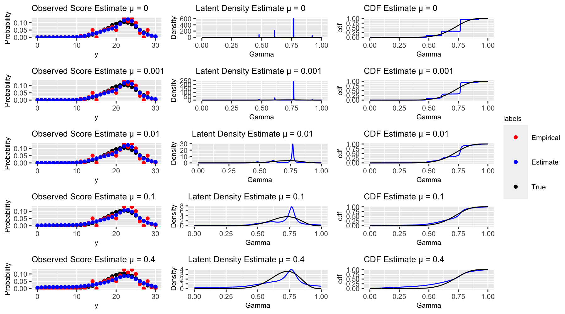
As we see, in Figure 10 the case of no regularization, when the empirical distribution $\widehat{p}$ is outside of $\text{conv}(\Gamma)$ , the NPMLE consists only of point masses, as the closest point $\widehat{p}_{MA}$ exists on the boundary of $\text{conv}(\Gamma)$ . However, as we increase $\mu$ , the latent distribution becomes smoother in the neighbourhood of each of these masses.

F Additional analysis on the NACC data

In this section we apply the selection methods for $p_{A}$ and $\mu$ to the NACC dataset.

As outlined in the main paper we first plot the intrinsic variability $||{\widehat{q}-\widehat{q}_{(A)}}||_{TV}$ as a function of the measurement assumption model for both the MOCA and the MMSE scores. From figures 11,12 the we pick the binomial model for the MMSE and the Laplace $h=1.34$ model for the MOCA model, though we also note the Gaussian and binomial models achieved very similar distance to the intrinsic variability distributions (for particular choices of $h$ ). We find each of the selected models have p-values of 1 in the first and second order feasibility tests.

Next as outlined in the main paper as we choose the regularization parameters for each branch of the model, $\mu_{Y}$ and $\mu_{Z}$ , corresponding to the MMSE and MOCA latent distributions. These are chosen using the procedure outlined in the main paper, here we plot the 2-observation likelihood as a function of the regularization parameter.

From our procedure in figures 13,14 we select $\mu_{Y}=0.0055,\mu_{Z}=0.0113$ for our model.

Lastly, we computed the cross entropy on the crosswalk (fully observed) dataset. Once again, we fix the selected measurement model $p_{A}$ on $Y$ and plot the cross entropy as a function of the conditional model or alternative method. The parametric model is the logit-normal model introduced in section A, the Z-score matching method is a currently used method for score conversion introduced in the main paper. As seen in the main paper, the overall optimal model is shown with the red x and the model we select without viewing any complete cases is shown in blue. We can observe that the smoothed non-parametric tends to produce the best conversions. Conversions using a compact support kernel can perform poorly if they don’t assign any probability to an observed value, however, we see that this can be partially combated through regularization. The parametric model tends to also perform well, though not under the selected $p_{A}$ . This may be partially explained by the tendency of variational inference methods to underestimate variances Bishop 2004. Noticing the improved performance of the parametric model under a larger $h$ seems to support this idea.

	$\displaystyle\phi_{\gamma\to\zeta}(q\|x)$	$\displaystyle=G^{-1}\left(F(q\|x)\|x\right)$		(2)
	$\displaystyle\phi_{\zeta\to\gamma}(q\|x)$	$\displaystyle=F^{-1}\left(G(q\|x)\|x\right)=\phi^{-1}_{\gamma\to\zeta}(q\|x)$		(3)

	$\displaystyle G(q\|x)$	$\displaystyle=P(\zeta\leq q\|x)$
		$\displaystyle=P(\phi_{\gamma\to\zeta}(\gamma\|x)\leq q\|x)$
		$\displaystyle=P(\gamma\leq\phi^{-1}_{\gamma\to\zeta}(q\|x)\|x)$
		$\displaystyle=F(\phi^{-1}_{\gamma\to\zeta}(q\|x)\|x)$
	$\displaystyle\implies\phi^{-1}_{\gamma\to\zeta}(q\|x)$	$\displaystyle=F^{-1}(G(q\|x)\|x)\text{ and }\phi_{\gamma\to\zeta}(q\|x)=G^{-1}(F(q\|x)\|x)$

	$\displaystyle\ell_{n,\mu}[P_{M}]$	$\displaystyle=\sum_{y=0}^{N}\widehat{p}(y)\log\left(\int p_{A}(y\|\gamma)p_{M}(\gamma)d\gamma\right)-\mu\mathcal{D}(P_{U}\|\|P_{M})$
		$\displaystyle=\sum_{y=0}^{N}\widehat{p}(y)\log\left(p_{MA}(y)\right)-\mu\mathcal{D}(P_{U}\|\|P_{M})$
		$\displaystyle=\sum_{y=0}^{N}\widehat{p}(y)\left(\log\left(p_{MA}(y,\gamma)\right)-\log\left(p_{MA}(\gamma\|y)\right)\right)-\mu\mathcal{D}(P_{U}\|\|P_{M})$
		$\displaystyle=\sum_{y=0}^{N}\widehat{p}(y)\int(p_{MA}^{(j)}(\gamma\|y)\left(\log\left(p_{MA}(y,\gamma)\right)-\log\left(p_{MA}(\gamma\|y)\right)\right)d\gamma-\mu\mathcal{D}(P_{U}\|\|P_{M})$
		$\displaystyle=Q[P_{M}\|\|P^{(j)}_{M}]+H[P_{M}\|\|P^{(j)}_{M}]-\mu\mathcal{D}(P_{U}\|\|P_{M}),$

	$\displaystyle p_{MA}(y,\gamma)$	$\displaystyle=p_{A}(y\|\gamma)p_{M}(\gamma),\quad p_{MA}(\gamma\|y)=\frac{p_{MA}(y,\gamma)}{p_{MA}(y)}$
	$\displaystyle Q[P_{M}\|\|P^{(j)}_{M}]$	$\displaystyle=\sum_{y=0}^{N}\widehat{p}(y)\int p_{MA}^{(j)}(\gamma\|y)\log\left(p_{MA}(y,\gamma)\right)d\gamma,$
	$\displaystyle H[P_{M}\|\|P^{(j)}_{M}]$	$\displaystyle=-\sum_{y=0}^{N}\widehat{p}(y)\int p_{MA}^{(j)}(\gamma\|y)\log\left(p_{MA}(\gamma\|y)\right)d\gamma$

$\displaystyle p_{\widehat{M}(\mu)}(\cdot\|x)$	$\displaystyle=\argmax_{p_{M}\in\mathcal{P}_{[0,1]}}\sum\widehat{p}(y\|x)\log\left(\int p_{A}(y\|\gamma)p_{M}(\gamma\|x)d\gamma\right)+\mu\int\log\left(p_{M}(\gamma\|x)\right)d\gamma$
$\displaystyle p_{\widehat{M}(\mu)A}(Y_{1},Y_{2}\|X)$	$\displaystyle=\int p_{A}(Y_{1}\|\gamma)p_{A}(Y_{2}\|\gamma)p_{\widehat{M}(\mu)}(\gamma\|X)d\gamma$
$\displaystyle\ell_{2}(p_{\widehat{M}(\mu)})$	$\displaystyle=\frac{1}{n_{2}}\sum_{i=1}^{n_{2}}\left[\log(p_{\widehat{M}(\mu)A}(Y_{i1},Y_{i2}\|X_{i}))\right]$	(11)

Data Harmonization Via Regularized Nonparametric Mixing Distribution Estimation

Supplement to: Data Harmonization Via Regularized Nonparametric Mixing Distribution Estimation

Contents

1 Introduction

2 Methods

Definition 2.1 (Harmonizable Variables).

Theorem 2.2.

2.1 Measurement Assumption Model

2.2 Latent Trait Models

2.2.1 Non-Parametric Model

Theorem 2.3.

2.2.2 Regularized Nonparametric Latent Trait

Theorem 2.4.

2.2.3 Incorporating covariates

2.3 Score Conversion

3 Model diagnostics and model selection with multiple observations

3.1 Feasibility test of the measurement assumption model

3.1.1 Multinomial Concentration and higher-order tests

3.2 Selection of the Measurement Assumption model using consecutive observations

3.3 Selection of μ\mu

4 Simulations

4.1 Intrinsic Variability Matching

4.2 Selecting the regularization tuning parameter

4.3 Performance of score conversion

4.4 Feasibility Tests

5 Application to the NACC data

6 Discussion

References

Acknowledgements

Supplementary Material

A A Parametric Model for the Latent Mixture

Supplemental Theorem A.1.

Supplemental Theorem A.2.

B Proofs of Supplemental Theorems

Proof of Supplemental Theorem A.1

Proof of Supplemental Theorem A.2

C Proofs of Main Paper Theorems

Theorem C.1.

Lemma C.2.

Theorem C.3.

Lemma C.4.

Lemma C.5.

Lemma C.6.

D Computational Details

Nonparametric EM sampling

E Additional simulations

E.1 Comparison: NPEM vs GP

E.2 Recovering p⁡(y)p(y) and pM​(γ)p_{M}(\gamma)

F Additional analysis on the NACC data

3.3 Selection of $\mu$

E.2 Recovering $p(y)$ and $p_{M}(\gamma)$