Non-Randomness of Google’s Quantum Supremacy Benchmark
Abstract
The first achievement of quantum supremacy has been claimed recently by Google for the random quantum circuit benchmark with 53 superconducting qubits. Here, we analyze the randomness of Google’s quantum random-bit sampling. The heat maps of Google’s random bit-strings show stripe patterns at specific qubits in contrast to the Haar-measure or classical random-bit strings. Google’s data contains more bit 0 than bit 1, i.e., about 2.8% difference, and fail to pass the NIST random number tests, while the Haar-measure or classical random-bit samples pass. Their difference is also illustrated by the Marchenko-Pastur distribution and the Girko circular law of random matrices of random bit-strings. The calculation of the Wasserstein distances shows that Google’s random bit-strings are farther away from the Haar-measure random bit-strings than the classical random bit-strings. Our results imply that random matrices and the Wasserstein distance could be new tools for analyzing the performance of quantum computers.
Quantum computers could simulate nature better than classical computers, as Feynman initiated the idea of quantum computing Feynman 1982. Quantum supremacy Preskill 2012; Harrow and Montanaro 2017 that a quantum computer could perform certain computational tasks exponentially faster than a classical computer, is one of key milestones in developing practical quantum computers. The power of a quantum computer is believed to stem from its quantum nature such as interference, entanglement, and a large Hilbert space growing exponentially with the number of qubits. The speed-up of quantum algorithms such as Shor’s factoring algorithm Shor 1997 or the Harrow-Hassidim-Lloyd algorithm for solving linear systems of equations Harrow et al. 2009 requires a large-scale and error-corrected quantum computer. With noisy-intermediate scale quantum computers available these days, quantum sampling algorithms are considered good candidates to demonstrate quantum supremacy or quantum advantage Bouland et al. 2019.
Recently, the achievements of quantum supremacy for quantum sampling algorithms on noisy intermediate scale quantum computers have been reported. In 2019, Google team Arute et al. 2019 claimed the first quantum supremacy by implementing random quantum circuits on 53 superconducting qubits. More recently, Wu et al. performed the random quantum circuits with 56 superconducting qubits Wu et al. 2021. In 2020, Zhong et al. Zhong et al. 2020 reported the quantum advantage in the Gaussian boson sampling on linear optical quantum computers. The boson sampling task is to sample bit strings from the probability distribution of bosons, given by the permanent of a unitary operator Troyansky and Tishby 1996; Aaronson and Arkhipov 2013.
Google’s quantum supremacy benchmark task is to generate random bit-strings by applying random quantum circuits on qubits followed by the measurement. The probability distribution of random bit-strings generated by random quantum circuits is not given by a uniform random distribution, but obeys the eigenvector distribution of a circular unitary ensemble Dyson 1962; Kuś et al. 1988. Google’s Sycamore quantum processor could generate millions of these random bit-strings of size in about 200 seconds, while a supercomputer with the currently known efficient classical algorithms would take much longer time Pednault et al. 2019; Huang et al. 2020. To verify that a quantum computer implements random quantum circuits correctly, the linear cross-entropy benchmark was introduced Arute et al. 2019; Neill et al. 2018. The linear cross-entropy fidelity is calculated using a probability distribution obtained from a classical computer and output bit-strings of a quantum computer. Its value was slightly greater than the theoretical threshold. However, there are important questions unexplored whether Google’s quantum random bit-strings are truly random, or how far away Google’s random bit-strings are from classical random bit-strings or from the Haar-measure sampling. A rigorous analysis is needed to quantify the performance of quantum random circuits because random unitary dynamics is essential in chaotic scattering Haake and Życzkowski 1990; Blümel and Smilansky 1990; Beenakker 1997; Haake et al. 2010; Livan et al. 2018, quantum information processing Emerson et al. 2003, randomized benchmarking of noisy quantum gates Emerson et al. 2005; Knill et al. 2008; Magesan et al. 2011, scrambling of information in black holes and quantum many-body systems Hayden and Preskill 2007; Nahum et al. 2018, and hydrodynamic simulation Richter and Pal 2021 in addition to the quantum supremacy benchmark test.
In this paper, we analyze the randomness of output bit-strings of random quantum circuits using the random matrix theory Mehta 2004; Livan et al. 2018; Tao and Vu 2015, the NIST random number test code Bassham et al. 2010, and the Wasserstein distance Villani 2008. To compare with the dataset of Google’s quantum supremacy experiment, classical random bit-strings and the Haar-measure random bit-strings are generated. The heat map patterns of random bit-strings and the NIST random number tests will show the non-randomness of Google’s random bit-strings and uncover errors of Google’s random quantum circuits. The difference between Google’ and classical random bit-strings is illustrated by the positions of outliers of random matrices of random bit-strings. Finally, we’ll calculate the Wasserstein distance between various data sets of random bit-strings. It will be shown that Google’s random bit strings are farther away from the Haar-measure random-bit strings than the classical random bit-strings
Random Quantum Circuits
Let us start with a brief introduction to the random quantum circuit benchmark and how to veryfy its faithful implementation. The random quantum circuit benchmark starts with samping a random unitary operator , then applying it on an input state of qubits and measuring the output state in the computational basis to generate the random bit string with . The probability of getting a random bit string is given by . By repeating this process times, a random-bit array is obtained.
The first key element of the random quantum circuit is how to draw unitary operators uniformly and randomly. Mathematically, this could be done with the Haar invariant measure on a unitary group. The collection of these random unitary operators is called a circular unitary ensemble (CUE) introduced by Dyson Dyson 1962. The Haar-measure sampling of a unitary operator out of the unitary group is challenging. A unitary operator can be decomposed into the product of 2-dimensional unitary transformations, called the Hurwitz decomposition Hurwitz 1963; Zyczkowski and Kuś 1994. However, this decomposition requires a huge amount of gate operations: the number of 1 or 2-qubit gates is and the number of parameters is . Emerson et al. Emerson et al. 2003 proposed a method of generating pseudo-random unitary operators: the quantum circuit of random unitary rotations on single qubits with parameters followed by the simultaneous two-body interactions on qubits are repeated times. On a classical computer, random unitary matrices can be generated by the QR decomposition of matrices with Gaussian random complex elements Mezzadri 2007. The QR algorithm needs floating point operations.
The second key element of the random quantum circuit is the statisical property of the probability finding a qubit state in . Random unitary operators make qubit states distributed uniformly in a dimensional Hilbert space. So amplitudes of may have the Gaussian distribution on the surface of a dimensional sphere. This leads to calculate the probability distribution for the random variable (dropping the subscript of )
| (1) |
This is the chi-square distribution wiht 2 degrees of freedom , and known as the eigenvector distribution of a circular unitary ensemble Kuś et al. 1988; Haake and Życzkowski 1990; Haake et al. 2010, For large , it becomes . Note that this should not be confused with the Porter-Thomas distribution that is the eigenvector distribution of an orthogonal circular ensemble Porter and Thomas 1956; Haake et al. 2010; Boixo et al. 2018; Neill et al. 2018; Arute et al. 2019. The expectation value of finding with respect to is given by . This is consistent with our intuition that classically the probability of finding a bit string out of possible bit strings is .
The last key element is to verify the faithful implementation of random quantum circuits. To this end, one has to estimate the empirical probability of finding a random quantum state in with from the output data, a random binary array. Then one has to construct an empirical probability of probabilities to compare it to the ideal probability given by Eq. (1). For a small number of qubits, the Kullback-Leibler divergence or the cross entropy of from were used to measure how the probability distribution is close to the ideal distribution Boixo et al. 2018; Neill et al. 2018.
However, in Google’s quantum supremacy experiment with qubits, the reconstruction of was impossible because a few millions of random bit-strings is too small to estimate with . Instead, the linear cross-entropy fidelity is introduced Boixo et al. 2018; Bouland et al. 2019; Arute et al. 2019; Aaronson and Chen 2017; Aaronson and Gunn 2020. Here, are the observed bit strings and the probability is calculated using the Schrödinger-Feyman simulation of a single random unitary operator for on on a supercomputer. A tricky point is that Google’s experiment applied the same single random unitary operator, rather than the CUE, to get a few millions of random bit-strings and to calculate on a supercomputer. If the CUE were used, would be random and the linear cross-entropy would not be applied. Google obtained for qubits.
Non-randomness of Google’s Random Bit Strings


Google’s measurement data sets Martinis et al. 2021 are the text files of random-bit arrays labeled by five parameters: n the number of qubits from 12 to 53, m the number of cycles from 12 to 20, s a seed for the pseudo-random number generator, e the elided gate number, and the two types of coupler activation patterns (EFGH or ABCDCDAB). The numbers of measurements are , , or . One example of Google’s data file is measurements_n53_m20_s0_e0_pABCDCDAB.txt.
The measurement data, random bit-strings, are the only information to tell whether the random quantum circuit benchmark was implemented properly on Google sycamore qubits. For comparison with Google’s random bit-strings, we generate (i) random bit-strings sampled from a circular unitary ensemble, called the CUE random bit-strings or the Haar measure random bit-strings, and (ii) classical random bit-strings. The CUE random bit-strings are generated by the QR decomposition algorithm Mezzadri 2007. A random matrix with complex elements sampled from the normal distribution is factored as , and then is a Haar measure unitary matrix. Due to the limited computing power of a personal computer, the CUE random-bit strings for are generated using Python or Julia random matrix library Chen et al. 2019. The classical random bit-strings from to are sampled using the pseudo-random number generator on a personal computer. The Python scripts generating the CUE and classical random bit-strings are attached in Supplementary.
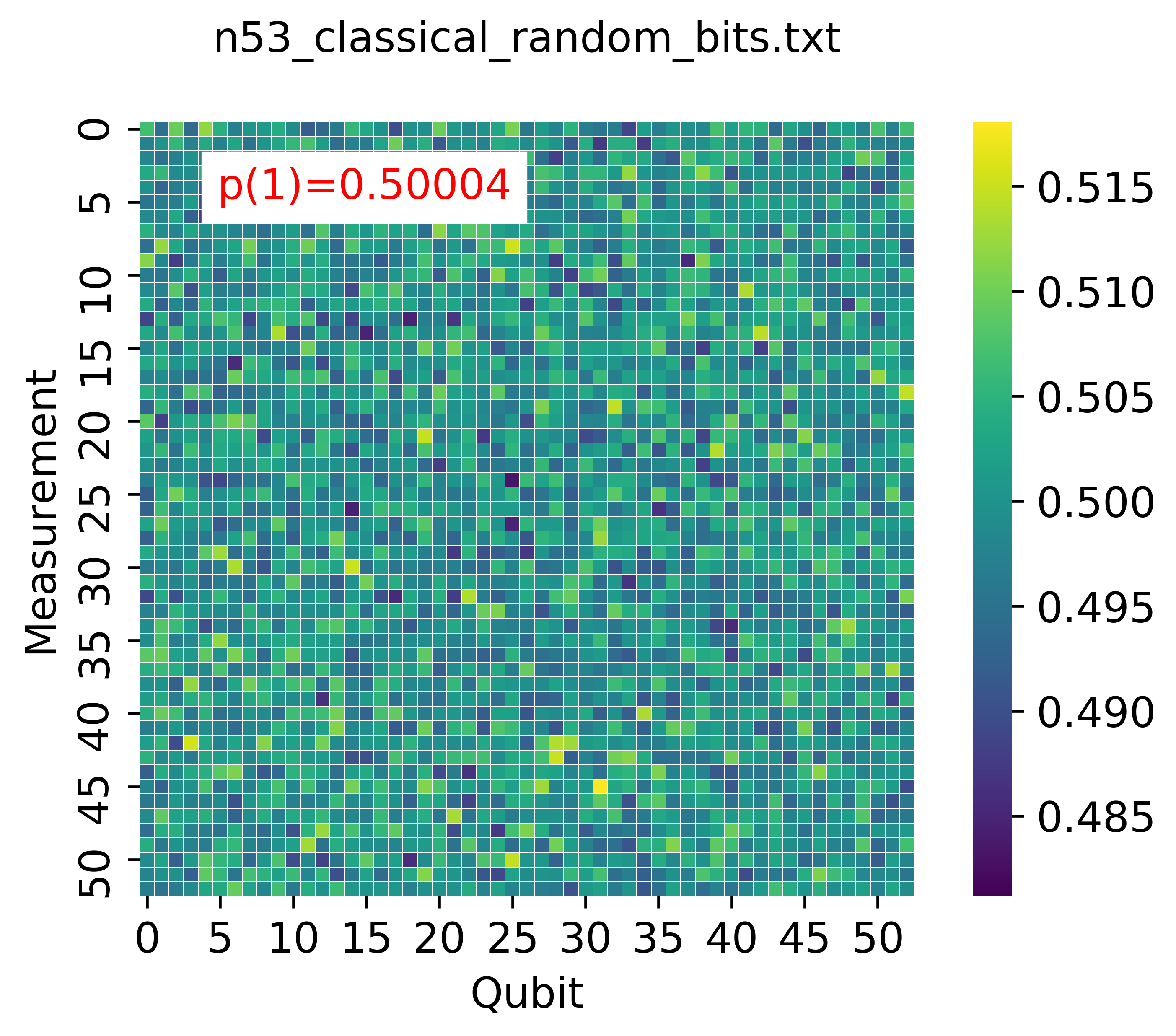
First, we plot the heat maps of random bit-strings as shown in Fig. 1. By slicing a rectangular array of random bit-strings, , the ensemble of square random binary matrices is constructed. Here is the -th row of the random bit array and . Figs. 1 (a), (b), and (c) show the heat maps of the average density matrix, with for Google, CUE, and classical random bit-strings, respectively. The heat maps for other Google samples from to and classical random bit-strings for are shown in Figs. S2, S3, S4 in Supplementary. Surprisingly, all the heat maps of Google’s data show the stripe patterns at some qubit indices, while the CUE and classical samples do not. As depicted Figs. S2, S3, and S4 in Supplementary, the two coupler activation types, EFGH and ABCDCDAB give rise to the different the bright and dark stripe patterns. For and ABCDCDAB activation, the stripe patterns become more clear as the cycle number increases. The total number of bit 1 of is counted to calculate the average of finding bit 1, . As shown in Figs. 1 (a), (b), and (c), Google’s random bit-strings show the vale , that is less than the expected value , while the CUE and classical random bit-strings have very close to 0.5. As shown in Figs. S2, S3, S4, for Google’s random bit strings ranges from 0.483 to 0.489. The non-randomness of Google’s random bit-strings can also be checked with a random number test, as well as the stripe patterns. We perform the NIST statistical random number tests Bassham et al. 2010; Ang 2019. As shown in Table S1 in Supplementary, Google’s quantum random bit-strings fail to pass some NIST random number tests, while the CUE and classical random bit strings pass. The failure of the NIST frequency test means Google’s data has too many 0’s. Also Google’s data fail to pass some NIST tests. Thus, we demonstrate that Google’s random bit-strings are not truly random in contrast to the CUE or classical random bit-strings.
Next, we calculate the empirical distributions for , where counts the number of bit-strings with the value and in decimal notation. As illustrated in Figs. 1 (d), (e), and (f), Google’s random bit-strings fluctuate widely and the classical random bit-strings fluctuate a little. Using the empirical distribution , one can construct the three empirical probability distributions , , and to see they follow Eq. (1), the eigenvector distribution of the circular unitary ensemble, as shown in Fig. 1 (g), (h), and (i). All three distributions are different from the eigenvector distribution of the CUE, Eq. (1). We leave the study of these discrepancies as an open question.

The difference between Google random bit-strings and the CUE or classical random bit-strings is further illustrated using the random matrix theory of the random binary matrices. The collection of matrices of random bit-strings can be regarded as a real Ginibre ensemble. It is well known that for random matrices with identically-and-independently matrix elements and zero mean, the distribution of complex eigenvalues of random matrices follows the Girko circular law Girko 1985; Tao and Vu 2015. However, random matrices formed by random bit strings here have the matrix element , so the mean of a matrix is not zero. If are sampled identically and independently from the Bernoulli distribution, the mean of could be . We are interested in whether the mean of generated by quantum random circuits is identical to 1/2 or not.
The distribution of the complex eigenvalues of random matrices with are plotted in Fig. 2. Most eigenvalues of both Google and classical random matrices are distributed inside of the circle with radius 1/2 and some outliers with large real eigenvalues are located outside the circle. As shown in Fig. 2 closely, the positions of outliers with large real eigenvalues of Google’s random bit-strings are different from that of the classical random bit-strings. The radius 1/2 and the outliers can be explained as follows. The matrix with nonzero mean can be transformed to with zero mean by
| (2) |
where is an all-one matrix. The ensemble of real random square matrices with the matrix elements sampled identically and independently from the Bernoulli distribution with zero mean and unit variance. The complex eigenvalues of are distributed uniformly in the unit circle. So the radius of the circle of the eigenvalue distribution of is 1/2. The Saturn-ring effect along the real line and the outliers shown in Fig. 2 are due to the fact that and are non-commutative.

Let us slice the random bit-string array into rectangular binary matrices where . Then, the collection of symmetric matrices is called the Wishart ensemble. It is known that if the elements of are sampled identically and independently from the normal distribution with zero mean and the variance , the distribution of real eigenvalues of is given by the Marchenko-Pastur distribution Marchenko and Pastur 1967
| (3) |
where are the upper and lower bounds and is the rectangular ratio. Here we take . Fig. 3 plots the Marchenko-Pastur distributions of Google’s and classical random-bit strings for . As shown in Fig. 3, the outliers outside the Marchenko-Pastur distribution distinguish Google’s random bit-strings from the classical random bit-strings. With Eq. (2), can be expressed as
| (4) |
Here the first term of Eq. (4) is be written as , so has zero mean and variance while the variance of is . This gives the upper and lower bounds, and , respectively. The last term of Eq. (4) becomes where an all-one matrix has the eigenvalue 0 and . So the outliers are located around .
How far away are they? – Wasserstein Distances

Up to now, we have shown (i) the non-randomness of Google’s random bit-strings using the heat maps and (ii) the random matrix theory of random bit-strings can distinguish Google’s data from the classical random samples. The final question we would like to address is how much Google random bit-strings are different from the CUE or classical random bit-strings. In Google’s experiment, the cross entropy fidelity was used to measure how the real distribution is close to the ideal distribution. The disadvantage of the cross entropy is that it is not symmetric and gives rise to zero or diverge if there is no overlap between two distributions. To overcome these, we employ the Wasserstein distance of order 1, between two discrete probability distributions, and ,
| (5) |
where is the joint probability of and such that , , and . Given two samples, and , can be obtained directly without calculating the empirical distributions and . We use the Python optimal transport library Flamary et al. 2021 for calculating the Wasserstein distance between two samples. Fig. 4 (a) plots the Wasserstein distances, normalized by , between Google and classical random bit-strings as a function of . For , Google samples with the activation pattern with EFGH are closer to the classical random bits than that with ABCDCDAB. For , we calculate the Wasserstein distance among all pairs of Google, CUE, and classical random bit-strings so their relative locations in the 2-dimension are displayed in Fig. 4 (b). It shows that Google random samples are farther away from the CUE random bit sample than the classical random bit sample. Also, all Google samples except 2 samples are fit to a straight line passing between the CUE and classical random bit samples.
Summary
In conclusion, we analyzed the randomness of Google’s quantum random bit-strings generated by random quantum circuits. It is found that the heat maps of Google’s data have the stripe patterns at specific qubit sites and contain more bit 0 than bit 1. This led to Google’s data failing to pass the NIST random number tests. These non-randomness signatures of Google bit strings do not occur in the Haar-measure random sample or in the classical random bit-strings. The non-randomness of Google’s data is caused by the errors of quantum gates or by the readout errors. The random matrices of random bit-strings distinguish Google data from the classical random bit-strings. The calculation of the Wasserstein distance shows that Google random bits are farther away from the Haar measure sample than the classical random bit sample. The Wasserstein distance between two samples would be a simple and powerful tool of measuring the fidelity of quantum gates. The two activation patterns of Google’s Sycamore qubits give rise to quite different results in the heat map of the bit strings and in the Wasserstein distances. Our findngs imply that the random matrix analysis and the Wasserstein distance may be used as benchmark tools to measure the performance of intermediate scale quantum computers. The linear cross-entropy used in Google’s supremacy experiment needs the classical simulation to calculate the probability of finding a bit-string . As the number of qubits increases, thise classical simulation is very difficult. So one faces the dilemma of how to veryfy the performance of quantum computers using the linear cross-entropy Eisert et al. 2020. The calculation of the Wasserstein distance requires only two data sets of bit-strings and do not need to estimate probability distributions from the two data sets. Classical random bit-strings for one hundred qubits can be easily generated and the Wasserstein distance between the classical random bit-strings and the random bit-strings of random quantum circuits could be calculated.
Acknowledgements
We would like to thank Seth Lloyd, Scott Aaronson, and Sergio Boixo for reading and commenting on our draft. Funding: This material is based upon work supported by the U.S. Department of Energy, Office of Science, National Quantum Information Science Research Centers. We also acknowledge the National Science Foundation under award number 1955907. Author contributions: S.K. led and coordinated the project. S.O. conceived the research idea and performed numerical calculations, All authors discussed the results and wrote the manuscript. Competing interests: The authors declare no competing interests. Data and material availability: All data and codes are provided in the main text or the supplementary materials.
References
- Feynman (1982) R. P. Feynman, International Journal of Theoretical Physics 21, 467 (1982).
- Preskill (2012) J. Preskill, Quantum computing and the entanglement frontier (2012), arXiv:1203.5813 [quant-ph] .
- Harrow and Montanaro (2017) A. W. Harrow and A. Montanaro, Nature 549, 203 (2017).
- Shor (1997) P. W. Shor, SIAM Journal on Computing 26, 1484 (1997).
- Harrow et al. (2009) A. W. Harrow, A. Hassidim, and S. Lloyd, Phys. Rev. Lett. 103, 150502 (2009).
- Bouland et al. (2019) A. Bouland, B. Fefferman, C. Nirkhe, and U. Vazirani, Nature Physics 15, 159 (2019).
- Arute et al. (2019) F. Arute, K. Arya, R. Babbush, D. Bacon, J. C. Bardin, R. Barends, R. Biswas, S. Boixo, F. G. S. L. Brandao, D. A. Buell, B. Burkett, Y. Chen, Z. Chen, B. Chiaro, R. Collins, W. Courtney, A. Dunsworth, E. Farhi, B. Foxen, A. Fowler, C. Gidney, M. Giustina, R. Graff, K. Guerin, S. Habegger, M. P. Harrigan, M. J. Hartmann, A. Ho, M. Hoffmann, T. Huang, T. S. Humble, S. V. Isakov, E. Jeffrey, Z. Jiang, D. Kafri, K. Kechedzhi, J. Kelly, P. V. Klimov, S. Knysh, A. Korotkov, F. Kostritsa, D. Landhuis, M. Lindmark, E. Lucero, D. Lyakh, S. Mandrà, J. R. McClean, M. McEwen, A. Megrant, X. Mi, K. Michielsen, M. Mohseni, J. Mutus, O. Naaman, M. Neeley, C. Neill, M. Y. Niu, E. Ostby, A. Petukhov, J. C. Platt, C. Quintana, E. G. Rieffel, P. Roushan, N. C. Rubin, D. Sank, K. J. Satzinger, V. Smelyanskiy, K. J. Sung, M. D. Trevithick, A. Vainsencher, B. Villalonga, T. White, Z. J. Yao, P. Yeh, A. Zalcman, H. Neven, and J. M. Martinis, Nature 574, 505 (2019).
- Wu et al. (2021) Y. Wu, W.-S. Bao, S. Cao, F. Chen, M.-C. Chen, X. Chen, T.-H. Chung, H. Deng, Y. Du, D. Fan, M. Gong, C. Guo, C. Guo, S. Guo, L. Han, L. Hong, H.-L. Huang, Y.-H. Huo, L. Li, N. Li, S. Li, Y. Li, F. Liang, C. Lin, J. Lin, H. Qian, D. Qiao, H. Rong, H. Su, L. Sun, L. Wang, S. Wang, D. Wu, Y. Xu, K. Yan, W. Yang, Y. Yang, Y. Ye, J. Yin, C. Ying, J. Yu, C. Zha, C. Zhang, H. Zhang, K. Zhang, Y. Zhang, H. Zhao, Y. Zhao, L. Zhou, Q. Zhu, C.-Y. Lu, C.-Z. Peng, X. Zhu, and J.-W. Pan, Strong quantum computational advantage using a superconducting quantum processor (2021), arXiv:2106.14734 [quant-ph] .
- Zhong et al. (2020) H.-S. Zhong, H. Wang, Y.-H. Deng, M.-C. Chen, L.-C. Peng, Y.-H. Luo, J. Qin, D. Wu, X. Ding, Y. Hu, P. Hu, X.-Y. Yang, W.-J. Zhang, H. Li, Y. Li, X. Jiang, L. Gan, G. Yang, L. You, Z. Wang, L. Li, N.-L. Liu, C.-Y. Lu, and J.-W. Pan, Science 370, 1460 (2020).
- Troyansky and Tishby (1996) L. Troyansky and N. Tishby, Permanent uncertainty: On the quantum evaluation of the determinant and the permanent of a matrix (1996).
- Aaronson and Arkhipov (2013) S. Aaronson and A. Arkhipov, Theory of Computing 9, 143 (2013).
- Dyson (1962) F. J. Dyson, Journal of Mathematical Physics 3, 1199 (1962).
- Kuś et al. (1988) M. Kuś, J. Mostowski, and F. Haake, Journal of Physics A: Mathematical and General 21, L1073 (1988).
- Pednault et al. (2019) E. Pednault, J. A. Gunnels, G. Nannicini, L. Horesh, and R. Wisnieff, Leveraging secondary storage to simulate deep 54-qubit sycamore circuits (2019), arXiv:1910.09534 [quant-ph] .
- Huang et al. (2020) C. Huang, F. Zhang, M. Newman, J. Cai, X. Gao, Z. Tian, J. Wu, H. Xu, H. Yu, B. Yuan, M. Szegedy, Y. Shi, and J. Chen, Classical simulation of quantum supremacy circuits (2020), arXiv:2005.06787 [quant-ph] .
- Neill et al. (2018) C. Neill, P. Roushan, K. Kechedzhi, S. Boixo, S. V. Isakov, V. Smelyanskiy, A. Megrant, B. Chiaro, A. Dunsworth, K. Arya, R. Barends, B. Burkett, Y. Chen, Z. Chen, A. Fowler, B. Foxen, M. Giustina, R. Graff, E. Jeffrey, T. Huang, J. Kelly, P. Klimov, E. Lucero, J. Mutus, M. Neeley, C. Quintana, D. Sank, A. Vainsencher, J. Wenner, T. C. White, H. Neven, and J. M. Martinis, Science 360, 195 (2018).
- Haake and Życzkowski (1990) F. Haake and K. Życzkowski, Phys. Rev. A 42, 1013 (1990).
- Blümel and Smilansky (1990) R. Blümel and U. Smilansky, Phys. Rev. Lett. 64, 241 (1990).
- Beenakker (1997) C. W. J. Beenakker, Rev. Mod. Phys. 69, 731 (1997).
- Haake et al. (2010) F. Haake, S. Gnutzmann, and M. Kuś, Quantum Signatures of Chaos (Springer-Verlag Berlin Heidelberg, 2010).
- Livan et al. (2018) G. Livan, M. Novaes, and P. Vivo, Introduction to Random Matrices – Theory and Practice (Springer International Publishing, 2018).
- Emerson et al. (2003) J. Emerson, Y. S. Weinstein, M. Saraceno, S. Lloyd, and D. G. Cory, Science 302, 2098 (2003), https://science.sciencemag.org/content/302/5653/2098.full.pdf .
- Emerson et al. (2005) J. Emerson, R. Alicki, and K. Życzkowski, Journal of Optics B: Quantum and Semiclassical Optics 7, S347 (2005).
- Knill et al. (2008) E. Knill, D. Leibfried, R. Reichle, J. Britton, R. B. Blakestad, J. D. Jost, C. Langer, R. Ozeri, S. Seidelin, and D. J. Wineland, Phys. Rev. A 77, 012307 (2008).
- Magesan et al. (2011) E. Magesan, J. M. Gambetta, and J. Emerson, Phys. Rev. Lett. 106, 180504 (2011).
- Hayden and Preskill (2007) P. Hayden and J. Preskill, Journal of High Energy Physics 2007, 120 (2007).
- Nahum et al. (2018) A. Nahum, S. Vijay, and J. Haah, Phys. Rev. X 8, 021014 (2018).
- Richter and Pal (2021) J. Richter and A. Pal, Phys. Rev. Lett. 126, 230501 (2021).
- Mehta (2004) M. L. Mehta, Random Matrices, Pure and Applied Mathematics, Vol. 142 (Elsevier, 2004).
- Tao and Vu (2015) T. Tao and V. Vu, The Annals of Probability 43, 782 (2015).
- Bassham et al. (2010) L. Bassham, A. Rukhin, J. Soto, J. Nechvatal, M. Smid, S. Leigh, M. Levenson, M. Vangel, N. Heckert, and D. Banks, A statistical test suite for random and pseudorandom number generators for cryptographic applications (2010).
- Villani (2008) C. Villani, Optimal Transport: Old and New, Grundlehren der mathematischen Wissenschaften (Springer Berlin Heidelberg, 2008).
- Hurwitz (1963) A. Hurwitz, Über die erzeugung der invarianten durch integration, in Mathematische Werke: Zweiter Band Zahlentheorie Algebra und Geometrie (Springer Basel, Basel, 1963) pp. 546–564.
- Zyczkowski and Kuś (1994) K. Zyczkowski and M. Kuś, Journal of Physics A: Mathematical and General 27, 4235 (1994).
- Mezzadri (2007) F. Mezzadri, NOTICES of the AMS 54, 592 (2007).
- Porter and Thomas (1956) C. E. Porter and R. G. Thomas, Phys. Rev. 104, 483 (1956).
- Boixo et al. (2018) S. Boixo, S. V. Isakov, V. N. Smelyanskiy, R. Babbush, N. Ding, Z. Jiang, M. J. Bremner, J. M. Martinis, and H. Neven, Nature Physics 14, 595 (2018).
- Aaronson and Chen (2017) S. Aaronson and L. Chen, in 32nd Computational Complexity Conference (CCC 2017), Leibniz International Proceedings in Informatics (LIPIcs), Vol. 79, edited by R. O’Donnell (Schloss Dagstuhl–Leibniz-Zentrum fuer Informatik, Dagstuhl, Germany, 2017) pp. 22:1–22:67.
- Aaronson and Gunn (2020) S. Aaronson and S. Gunn, On the classical hardness of spoofing linear cross-entropy benchmarking (2020), arXiv:1910.12085 [quant-ph] .
- Martinis et al. (2021) J. M. Martinis et al., https://doi.org/10.5061/dryad.k6t1rj8 (2021).
- Chen et al. (2019) J. Chen, S. Olver, J. Nash, A. Noack, C. Rackauckas, S. Micluța-Câmpeanu, K. Squire, A. Merberg, A. Edelman, T. Kelman, S. Schoelly, M. Schauer, A. Lamacraft, and A. Deshpande, Juliamath/randommatrices.jl: v0.5.0 (2019).
- Ang (2019) S. K. Ang, randomness_testsuite (2019).
- Girko (1985) V. L. Girko, Theory Probab. Appl. 29, 694 (1985).
- Marchenko and Pastur (1967) V. A. Marchenko and L. A. Pastur, Mat. Sb. (N.S.) 72, 507 (1967).
- Flamary et al. (2021) R. Flamary, N. Courty, A. Gramfort, M. Z. Alaya, A. Boisbunon, S. Chambon, L. Chapel, A. Corenflos, K. Fatras, N. Fournier, L. Gautheron, N. T. Gayraud, H. Janati, A. Rakotomamonjy, I. Redko, A. Rolet, A. Schutz, V. Seguy, D. J. Sutherland, R. Tavenard, A. Tong, and T. Vayer, Journal of Machine Learning Research 22, 1 (2021).
- Eisert et al. (2020) J. Eisert, D. Hangleiter, N. Walk, I. Roth, D. Markham, R. Parekh, U. Chabaud, and E. Kashefi, 2, 382 (2020).
Supplementary Materials for “Non-Randomness of Google’s Quantum Supremacy Benchmark”
.1 Preparation of the data and the script files
The three kinds of random bit strings used in this study are prepared as follows.
- •
Google’s data for quantum supremacy benchmark test Martinis et al. 2021 is downloaded from the Dryad Digital Repository,
https://datadryad.org/stash/dataset/doi:10.5061/dryad.k6t1rj8. - •
The QR algorithm is used to perform the Haar measure sampling of unitary operators from . The Python script and the Julia script, Haar.py and Haar.jl were written. Due to the limit of the computational power of the PC (Intel Core i7-4790 CPU @ 3.60 GHz and 24 GB memory), it took about 7 days to sample 60000 random unitary operators using the QR algorithm for .
- •
The classical random bit strings are generated using a simple Python script, Randbit.py. The classical random bit array of the size by is produced quickly within a few minutes on the PC.
.2 Eigenvalue distributions of the Haar measure samples
Fig. S1 shows the eigenvalue distributions of Haar measure samples of generated by the QR algorithm.

.3 Heat maps of Google random bit-strings
Figs. S2 and S3 show the heat maps of Google’s data from to with the activation pattern EGGH. Figs. S4 depicts the heat maps of Google’s data for , the cycles , and the activation pattern ABCDCDAB. The pictures are plotted by running the Python script, Heatmap.py, as follows


.4 NIST Statistical Test for Random Numbers
The randomness of Google’s random bit-strings are tested using the NIST statistical test suite for random and pseudo-random number
generators for cryptographic applications Bassham et al. 2010. Instead of the NIST C code, NIST SP 800-22,
the Python implementation of the NIST statistical test suite developed by Ang Ang 2019 is used because of the easy graphic
user-interface, as shown in Fig. S5. Table S1 shows the results of the NIST random number
tests for classical random bits for , Qiskit random circuits for , the Haar measure sample for ,
and Google’s data from to . Most Google’s data do not pass the frequency test, run test, and overlapping template
matching, approximate entropy test, and cumulative sum tests. We performed the NIST statistical test for all Google data and
the result files Random_test.zip are attached.

| 01. Frequency test (mono-bit) | 02. Frequency test within a block | 03. Run test | 04. Longest run of ones in a block | 05. Binary matrix rank test | 06. Discrete Fourier transform | 07. Non-overlapping template matching | 08. Overlapping Template Matching | 09. Maurer’s universal statistics | 10. Linear complexity test | 11. Serial test | 12. Approximate entropy test | 13. Cumulative sums test (forward) | 14. Cumulative sums test (reverse) | 15. Random excursions test | 16. Random excursions variant | |||
| CUE sampling, n=12 | R | R | R | R | R | R | R | R | R | R | R | R | R | R | R | R | ||
| random bit sampling, n=53 | R | R | R | R | R | R | R | R | R | R | R | R | R | R | R | R | ||
n12_m14_s0_e0_pEFGH |
N | N | N | R | R | R | N | N | R | R | U | N | N | N | R | R | ||
n14_m14_s0_e0_pEFGH |
N | N | N | R | R | R | N | N | N | R | U | N | N | N | R | R | ||
n16_m14_s0_e6_pEFGH |
N | N | N | R | R | R | N | N | R | R | U | N | N | N | R | R | ||
n18_m14_s3_e6_pEFGH |
N | N | N | R | R | R | N | N | R | R | N | N | N | N | R | R | ||
n20_m14_s3_e0_pEFGH |
N | N | N | R | R | R | N | N | R | R | R | N | N | N | R | R | ||
n22_m14_s0_e0_pEFGH |
N | N | N | R | R | R | N | N | R | R | R | N | N | N | R | R | ||
n24_m14_s0_e0_pEFGH |
N | N | N | N | R | R | N | N | R | R | U | N | N | N | R | R | ||
n26_m14_s0_e0_pEFGH |
N | N | N | R | R | R | N | N | R | R | R | N | N | N | R | R | ||
n28_m14_s0_e0_pEFGH |
N | N | N | R | R | R | N | N | R | R | U | N | N | N | U | R | ||
n30_m14_s0_e0_pEFGH |
N | N | N | R | R | R | N | N | R | R | R | N | N | N | R | R | ||
n32_m14_s0_e0_pEFGH |
N | N | N | N | R | R | N | N | N | R | R | N | N | N | R | R | ||
n34_m14_s0_e0_pEFGH |
N | N | N | R | R | R | N | N | R | R | R | N | N | N | R | R | ||
n36_m14_s0_e0_pEFGH |
N | N | N | R | R | N | N | N | N | R | U | N | N | N | R | R | ||
n38_m14_s0_e0_pEFGH |
N | N | N | R | R | R | N | N | R | R | R | N | N | N | R | R | ||
n39_m14_s0_e0_pEFGH |
N | N | N | N | R | R | N | N | R | R | U | N | N | N | U | R | ||
n40_m14_s0_e0_pEFGH |
N | N | N | N | R | R | N | N | R | R | U | N | N | N | R | R | ||
n41_m14_s0_e0_pEFGH |
N | N | N | N | R | R | N | N | R | R | R | N | N | N | R | R | ||
n42_m14_s3_e6_pEFGH |
N | N | N | N | R | R | N | N | R | R | U | N | N | N | R | R | ||
n43_m14_s0_e0_pEFGH |
N | N | N | N | R | N | N | N | R | R | U | N | N | N | R | R | ||
n44_m14_s0_e0_pEFGH |
N | N | N | R | R | R | N | N | N | R | R | N | N | N | R | R | ||
n45_m14_s0_e0_pEFGH |
N | N | N | N | R | R | N | N | R | R | R | N | N | N | R | R | ||
n46_m14_s0_e0_pEFGH |
N | N | N | N | R | R | N | N | R | R | U | N | N | N | R | R | ||
n47_m14_s0_e0_pEFGH |
N | N | N | R | R | R | N | N | R | R | U | N | N | N | R | R | ||
n48_m14_s0_e0_pEFGH |
N | N | N | N | R | R | N | N | N | R | U | N | N | N | R | R | ||
n49_m14_s0_e6_pEFGH |
N | N | N | R | R | R | N | N | R | R | U | N | N | N | R | R | ||
n50_m14_s0_e0_pEFGH |
N | N | N | R | R | R | N | N | N | R | U | N | N | N | R | R | ||
n51_m14_s0_e0_pEFGH |
N | N | N | N | R | R | N | N | R | R | U | N | N | N | R | R | ||
n53_m14_s0_e0_pEFGH |
N | N | N | R | R | R | N | N | R | R | U | N | N | N | R | R | ||
n53_m12_s1_e0_pABCDCDAB |
N | N | N | R | R | R | N | N | R | R | U | N | N | N | R | R | ||
n53_m14_s2_e0_pABCDCDAB |
N | N | N | N | R | R | N | N | R | R | U | N | N | N | U | U | ||
n53_m16_s0_e0_pABCDCDAB |
N | N | N | N | R | R | N | N | R | R | U | N | N | N | R | R | ||
n53_m18_s0_e0_pABCDCDAB |
N | N | N | N | R | R | N | N | R | R | N | N | N | N | U | R | ||
n53_m20_s0_e0_pABCDCDAB |
N | N | N | N | R | R | N | N | N | R | U | N | N | N | R | R | ||
n53_m20_s1_e0_pABCDCDAB |
N | N | N | R | R | R | N | N | R | R | U | N | N | N | R | R |