Intersection Bodies of Polytopes
Abstract
We investigate the intersection body of a convex polytope using tools from combinatorics and real algebraic geometry. In particular, we show that the intersection body of a polytope is always a semialgebraic set and provide an algorithm for its computation. Moreover, we compute the irreducible components of the algebraic boundary and provide an upper bound for the degree of these components.
1 Introduction

This paper studies intersection bodies from the perspective of real algebraic geometry.
Originally, intersection bodies were defined by Lutwak [Lut88] in the context of convex geometry.
In view of the notion of -dimensional cross-section measures
and the related concepts of associated
bodies (such as intersection bodies, cross-section bodies, and projection
bodies), intersection bodies play an essential role in geometric
tomography (see [Gar06, Chapter 8] and [Mar94, Section 2.3]). In particular, we mention here the Busemann-Petty
problem which asks if one can compare the volumes of two convex bodies by comparing the volumes of their sections [Gar94a, Gar94b, GKS99, Kol98, Zha99b].
Moreover, Ludwig showed that the unique non-trivial GL-covariant star-body-valued valuation on convex polytopes corresponds to taking the intersection body of the dual polytope [Lud06]. Due to such results, the knowledge on properties of
intersection bodies interestingly contributes
also to the (still not systematized) theory of starshaped sets, see
Section 17 of the exposition [HHMM20].
Recently, there is increased interest in investigating convex geometry from an algebraic point of view [BPT13, Sin15, RS10, RS11].
In this article,
we will focus on the intersection bodies of polytopes from this perspective. It is known that in , the intersection body of a centrally symmetric polytope centered at the origin is the same polytope rotated by and dilated by a factor of (see e.g. [Gar06, Theorem 8.1.4]). Moreover, if is a full-dimensional convex body in centered at the origin, then so is its intersection body [Gar06, Chapter 8.1].
But what do these objects look like in general? In , with , they cannot be polytopes [Cam99, Zha99a] and they may not even be convex. In fact, for every convex body , there exists a translate of such that its intersection body is not convex. This happens because of the important role played by the origin in the construction of the intersection body.
Our main contribution is Theorem 3.2, which states that the intersection body of a polytope is a semialgebraic set, i.e. a subset of defined by a boolean combination of polynomial inequalities. The proof relies on two key facts. First, the volume of a polytope can be computed using determinants. Second, the combinatorial type of the intersection of a polytope with a hyperplane is fixed for each region of a certain central hyperplane arrangement. In Section 2, we prove semialgebraicity for the intersection body of polytopes containing the origin, and we generalize the result to arbitrary polytopes in Section 3. In Section 4, we present an algorithm to compute the radial function of the intersection body of a polytope. An implementation is available at [MR21]. In Section 5, we describe the algebraic boundary of the intersection body, which is a hypersurface consisting of several irreducible components, each corresponding to a region of the aforementioned hyperplane arrangement. Theorem 5.6 gives a bound on the degree of the irreducible components. Section 6 focuses on the intersection body of the -cube centered at the origin (Figure 4(a)).
2 The Intersection Body of a Polytope is Semialgebraic
In convex geometry it is common to use functions in order to describe a convex body, i.e. a non-empty convex compact subset of . This can be done e.g. by the radial function. A more detailed introduction can be found in [Sch14].
Definition 2.1.
Given a convex body , the radial function of is
As a convention is when and it is otherwise. An immediate consequence of the definition is that for . Therefore, we can equivalently define the radial function on the unit sphere , and then extend to the whole space using the previously mentioned relation. Throughout this paper we will use the following convention: denotes a vector in whereas denotes a vector in . With the observation that we can restrict to the sphere, we define the intersection body of by its radial function, which is given by the volume of the intersections of with hyperplanes through the origin.
Definition 2.2.
Let be a convex body in . Its intersection body is defined to be the set where the radial function (restricted to the sphere) is
for . We denote by the hyperplane through the origin with normal vector , and by the -dimensional Euclidean volume, for .
We begin our investigation by considering the intersection body of polytopes which contain the origin. For instance, Figure 1 displays the intersection body of an icosahedron centered at the origin. If the origin belongs to the interior of the polytope , then is continuous and hence is also continuous [Gar06]. Otherwise we may have some points of discontinuity which correspond to unit vectors such that contains a facet of ; there are finitely many such directions. The intersection body is well defined, but there may arise subtleties when dealing with the boundary. However, we will see later (in Remark 5.2) that for our purposes everything works out. In the following we use notions from polytope theory, such as zonotopes and combinatorial types. For further background on polytopes we refer the reader to [Zie95].
Example 2.3.
We will use the cube as an ongoing example to illustrate the key concepts used throughout the paper. Let be the -dimensional cube . If we intersect with hyperplanes , for , we can observe that there are two possible combinatorial types for : it is either a parallelogram (Figure 2(a)) or a hexagon (Figure 2(b)).


There are finitely many regions of the sphere for which the combinatorial type stays the same (see Lemma 2.4). Using this we can parameterize the area of the parallelogram or hexagon with respect to the vector to construct the radial function of . Indeed, as will be shown in the proof of Theorem 2.6, this can be equivalently written to provide a semialgebraic description of the intersection body. In particular, if the intersection is a square, then the radial function in a neighborhood of that point will be a constant term over a coordinate variable, e.g. . On the other hand, when the intersection is a hexagon, the radial function is a degree two polynomial over . The intersection body is convex as promised by the theory and displayed in Figure 4(a). We continue with this in Example 5.3.
Lemma 2.4.
Let be a full-dimensional polytope in . Then there exists a central hyperplane arrangement in whose maximal open chambers satisfy the following property. For all , the hyperplane intersects a fixed set of edges of and the polytopes are of the same combinatorial type.
Proof.
Let be a generic vector of and consider . The vertices of are the points of intersection of with the edges of . Perturbing continuously, the intersecting edges (and thus the combinatorial type) remain the same, unless the hyperplane passes through a vertex of . This happens if and only if and thus the set of normal vectors of such hyperplanes is given by Taking the union over all vertices yields the central hyperplane arrangement
Then each open region of the complement of contains points such that intersects a fixed set of edges of . ∎
The proof of Lemma 2.4 implies that the number of regions we are interested in is the number of chambers of the central hyperplane arrangement . Let where if . Then we have an upper bound for such a number:
given by the number of chambers of a generic arrangement [Sta07, Prop. 2.4].
Remark 2.5.
We note that there are several ways to view the hyperplane arrangement in Lemma 2.4. For example, since the vertices of are the normal vectors of the facets of the dual polytope , we can describe as the collection of linear hyperplanes which are parallel to facets of . We also note that is the normal fan of a zonotope whose edge directions are orthogonal to the hyperplanes of . The fan induced by the hyperplane arrangement is the normal fan of the zonotope
We will call this zonotope the zonotope associated to . As will be clarified later in Remark 5.9, the dual body of plays an important role in the visualization and the combinatorics of the intersection body .
Theorem 2.6.
Let be a full-dimensional polytope containing the origin. Then , the intersection body of , is semialgebraic.
Proof.
Fix a region for an open cone from Lemma 2.4. Then for every the hyperplane intersects in the same set of edges. Let be a vertex of . Then there is an edge of such that . This implies that for some and . From this we get that
which implies that
In this way we express as a function of (for fixed and ). Let be the vertices of and let be the corresponding edges of .
We now consider the following triangulation of :
first, triangulate each facet of that does not contain the origin, without adding new vertices (this can always be done e.g. by a regular subdivision using a generic lifting function, cf. [LRS10, Prop. 2.2.4]). For each -dimensional simplex in this triangulation, consider the -dimensional simplex with the origin. This constitutes a triangulation of , in which the origin is a vertex of every simplex.
Restricting to , the radial function of the intersection body in direction is the volume of , and hence given by
We can thus compute as
where
and the row vectors (along with the origin) are vertices of the simplex of the triangulation. Therefore, we obtain an expression for some polynomials without common factors, for . With the same procedure applied to all regions , for as in Lemma 2.4, we obtain an expression for that is continuous and piecewise a quotient of two polynomials . It follows from the definition of the radial function that
Notice that for every we have the following equality:
and therefore, if ,
Because the radial function is a semialgebraic map, by quantifier elimination the intersection body is also semialgebraic. More explicitly, let be the set of indices such that . Then we can write the intersection body as
This expression gives exactly a semialgebraic description of . ∎
Example 2.7.
Let be the regular icosahedron in , whose vertices are all the even permutations of . The associated hyperplane arrangement has chambers. The first type of chambers is spanned by five rays and the radial function of is given by a quotient of a quartic and a quintic, defined over . In the remaining twenty chambers is a quintic over a sextic, again with coefficients in . This intersection body is the convex set shown in Figure 1. We will continue the analysis of in Example 5.10.
The theory of intersection bodies assures that the intersection body of a centrally symmetric convex body is again a centrally symmetric convex body, as it happens in Example 2.3 and in Example 2.7. On the other hand, given any polytope (indeed this holds more generally for any convex body) there exists a translation of such that is not convex. This is the content of the next example.
Example 2.8.
Let be the cube , so that the origin is a vertex of . The hyperplane arrangement associated to divides the space in chambers. In two of them the radial function is . In six regions the radial function has the following shape (up to permutation of the coordinates and sign):
There are then regions in which the radial function looks like
In the remaining six regions we have
Figure 3 shows two different points of view of , which is in particular not convex.


3 Non-convex Intersection Bodies
The proof of Theorem 2.6 relies on the fact that the origin is in the polytope. However, if the origin is not contained in , we can still find a semialgebraic description of by adjusting how we compute the volume of . The remainder of this section will be dedicated to proving this.
Lemma 3.1.
Let be a full-dimensional polytope, and let be the set of its facets. Let be a point outside of . For each face , let denote the set . Then the following equality holds:
where is if and belong to the same halfspace defined by , and otherwise.
Proof.
Let and denote by the set of facets of for which the halfspace defined by containing also contains , possibly on its boundary. Let .
First we will show that . The inclusion follows immediately from convexity. To see the opposite direction, let and consider to be the ray starting at and going through . Either intersects only along its boundary, or there are some intersection points also in the interior of . In the first case and so for some face , that by convexity must be in . On the other hand, if the ray intersects the interior of the polytope , denote by the farthest among the intersection points:
Let be a facet containing . Then, is contained in the convex hull of , i.e. . From the definition of it follows that the halfspace defined by containing must also contain , so and our statement holds.
Next, we will show that . The pyramid is contained in the closed halfspace defined by which contains . By the definition of , this halfspace does not contain thus . Also, so we have that and hence . Conversely, let . If we are done, so assume . Then, for some , . Let be the point at which the segment from to first intersects the boundary of , i.e.
Then by construction there exists a facet containing , such that . Thus, we have that
If and or , then the volume of is zero, therefore
and the claim follows. ∎
Theorem 3.2.
Let be a full-dimensional polytope. Then , the intersection body of , is semialgebraic.
Proof.
What remains to be shown is that is semialgebraic in the case when the origin is not contained in , and hence it is not contained in any of its sections . From Lemma 3.1, with we have that
where is the convex hull of and the origin. Let be a triangulation of . We can calculate as in the proof of Theorem 2.6
where is the matrix whose rows are the vertices of the simplex and . We then follow the remainder of the proof of Theorem 2.6 to see that the intersection body is semialgebraic. ∎
4 The Algorithm
The proofs from Theorem 2.6 and Theorem 3.2 lead to an algorithm to compute the radial function of the intersection body of a polytope.
In this section, we describe the algorithm.
By Remark 2.5, the regions in which for fixed polynomials and are defined by the normal fan of the zonotope . First, we compute the radial function for each of these cones individually, by applying Algorithm 1.
This algorithm has as output the rational function .
Iterating over all regions yields the final Algorithm 2.
An implementation of these algorithms for SageMath 9.2 [Sag21] and Oscar 0.8.2-DEV [OSC22] can be found in https://mathrepo.mis.mpg.de/intersection-bodies. Note that in step 1 of Algorithm 1, the implementation uses a regular subdivision of the facets of the polytope by lifting the vertices along the moment curve with .
5 Algebraic Boundary and Degree Bound
In order to study intersection bodies from the point of view of real algebraic geometry we need to introduce our main character for this section, the algebraic boundary. For more on the algebraic boundary we refer the reader to [Sin15].
Definition 5.1.
Let be any compact subset in , then its algebraic boundary is the -Zariski closure of the Euclidean boundary .
Knowing the radial function of a convex body implies knowing its boundary. In fact, when then if and only if (see Remark 5.2 for the other cases). Therefore, using the same notation as in the proof of Theorem 2.6, we can observe that the algebraic boundary of the intersection body of a polytope is contained in the union of the varieties . Indeed, we actually know more: as will be proven in 5.5, the ’s are divisible by the polynomial , and hence
because of the assumption made in the proof of Theorem 2.6 that do not have common components. That is, these are exactly the irreducible components of the boundary of .
Remark 5.2.
As anticipated in Section 2 there may be difficulties when computing the boundary of in the case where the origin is not in the interior of the polytope . In particular, is a discontinuity point of the radial function of if and only if contains a facet of . Therefore has discontinuity points if and only if the origin lies in the union of the affine linear spans of the facets of . In this case, there are finitely many rays where the radial function is discontinuous and they belong to , i.e. to the hyperplane arrangement . If , these rays disconnect the space, and this implies that we loose part of the (algebraic) boundary of : to the set we need to add segments from the origin to the boundary points in the direction of these rays. However, in higher dimensions the discontinuity rays do not disconnect so approaches the region where the radial function is zero continuously except for these finitely many directions. Therefore there are no extra components of the boundary of .
Example 5.3 (Continuation of Example 2.3, cf. Figure 4(a)).
Starting from the radial function of the intersection body of the -cube , computed using Algorithm 1, we can recover the equations of its algebraic boundary. The Euclidean boundary of this convex body is divided in regions. Among them, arise as the intersection of a convex cone spanned by rays with a hyperplane; they constitute facets, i.e. flat faces of dimension , of . For example the facet exposed by the vector is the intersection of with the convex cone
In other words, the variety is one of the irreducible components of . The remaining regions are spanned by rays each, and the polynomial that defines the boundary of is a cubic, such as
in the region
These cubics are in fact, up to a change of coordinates, the algebraic boundary of a famous spectrahedron: the elliptope [LP95]. Hence is the union of irreducible components, six of degree and eight of degree .
Remark 5.4.
In [PSW21] the authors introduce the notion of patches of a semialgebraic convex body, with the purpose of mimicking the faces of a polytope. In the case of intersection bodies of polytopes, it is tempting to think that each region of Lemma 2.4 corresponds to a patch. Indeed, this happens, for example, for the centered -cube in Example 5.3. On the other hand, if then there are regions that define the same patch of the algebraic boundary of ; therefore there is, unfortunately, no one-to-one correspondence between regions and patches.
Proposition 5.5.
Using the notation of Lemma 2.4 and Theorem 3.2, fix a chamber of and let for some . Then the polynomial divides and
Proof.
For the fixed region , let be a triangulation of with simplices indexed by . Then the volume of is given by
where is the matrix as in the proof of Theorem 2.6. Notice that for each , we can rewrite the determinant to factor out a denominator (we also write for simplicity ):
where
and the determinant of is a polynomial of degree in the ’s. Note that if we multiply we obtain the vector . Hence if , then , i.e. the kernel of is non-trivial and thus . This implies the containment of the complex varieties and therefore the polynomial divides the polynomial . When we sum over all the simplices in the triangulation we obtain that
and
Hence and , so the claim follows. ∎
Notice that generically, meaning for the generic choice of the vertices of , the bound in 5.5 is attained, because and will not have common factors.
Theorem 5.6.
Let be a full-dimensional polytope with edges. Then the degrees of the irreducible components of the algebraic boundary of are bounded from above by
Proof.
We want to prove that , for every , .
By definition, every vertex of is a point lying on an edge of , so trivially . We want to argue now that it is impossible to intersect more than edges of with our hyperplane . If the origin is one of the vertices of , then all the edges that have the origin as a vertex give rise only to one vertex of : the origin itself. There are at least such edges, because is full-dimensional, and so .
Suppose now that the origin is not a vertex of , then does not contain vertices of . It divides in two half spaces and , and so it divides the vertices of in two families of vertices in and vertices in . Either or are equal to , or they are both greater than one. In the first case let us assume without loss of generality that , i.e. there is only one vertex in . Then pick one vector in : because is a full-dimensional polytope, there are at least edges of with as a vertex. Only one of them may connect to and therefore the other edges must lie in . This gives .
On the other hand, let us assume that . Then there is at least one edge in and one edge in . If these are the edges that do not intersect the hyperplane. For we reason as follows. Suppose that intersects a facet of . Then it cannot intersect all the facets of (i.e. a ridge of ), otherwise we would get which contradicts the fact that does not intersect vertices of . So there exists a ridge of that does not intersect the hyperplane; it has dimension and therefore it has at least edges. Therefore
∎
Corollary 5.7.
In the hypotheses of Theorem 5.6, if is centrally symmetric and centered at the origin, then we can improve the bound with
Proof.
We already know that for each chamber from Lemma 2.4, the degree of the corresponding irreducible component is bounded by the degree of the polynomial . This follows from the construction of and in the proof of Theorem 2.6. Specifically, the determinant which gives comes with the product of rational functions, with linear numerator and denominators, and one linear term. Thus which implies that . By definition these polynomials are obtained as the least common multiple of objects with shape
If is centrally symmetric, so is , and therefore we have the vertex belonging to the edge and also the vertex belonging to the edge . When computing the least common multiple, these two vertices produce the same factor, up to a sign, and therefore they count as the same linear factor of . Hence for every
∎
Example 5.8.
Let be the tetrahedron in with vertices , . The associated hyperplane arrangement coincides with the one associated to the cube in Example 5.3, so it has chambers that come in two families.
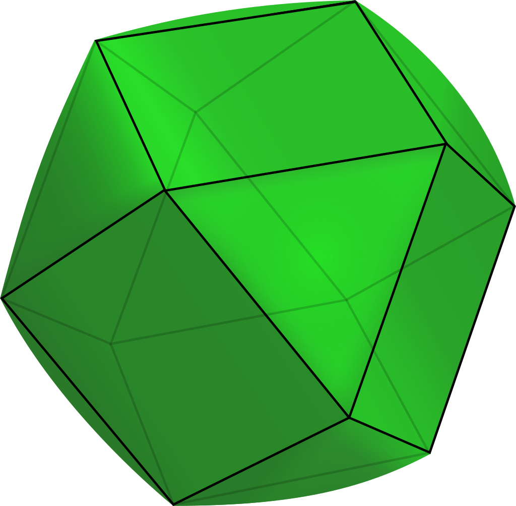


The first one consists of cones spanned by four rays, such as (see Example 5.3). The polynomial that defines the boundary of in this region is a quartic, namely
On the other hand the cones of the second family are spanned by three rays: here the section of is a triangle and the equation of the boundary if is a cubic. An example is the cone with the polynomial
Note that this region furnishes an example in which the bounds given in 5.5 and Theorem 5.6 are attained.
Remark 5.9.
Remark 2.5 together with 5.5 implies that the structure of the irreducible components of the algebraic boundary of is strongly connected with the face lattice of the dual of the zonotope . More precisely, in the generic case, the lattice of intersection of the irreducible components is isomorphic to the face lattice of the dual polytope . Thus, a classification of “combinatorial types” of such intersection bodies is analogous to the classification of zonotopes / hyperplane arrangements / oriented matroids. It is however worth noting, that the same zonotope can be associated to two polytopes and which are not combinatorially equivalent. One example of this instance is a pair of polytopes such that and , as can be seen in Figure 4 for the cube and the tetrahedron. To have a better overview over the structure of the boundary of , one strategy is to use the Schlegel diagram of . We label each maximal cell by the degree of the polynomial that defines the corresponding irreducible component of , as can be seen in Figures 5 and 6.
Example 5.10 (Continuation of Example 2.7, cf. Figure 1).
Let be the regular icosahedron. In the regions which are spanned by five rays, the polynomial that defines the boundary of has degree and it looks like
In the other regions spanned by three rays, is the zero set of a sextic polynomial with the following shape

We visualize the structure of these pieces using the Schlegel diagram in Figure 5, where the numbers correspond to the degree of the polynomials, as explained in Remark 5.9.
Using this technique we are then able to visualize the boundary of intersection bodies of -dimensional polytopes via the Schlegel diagram of .
Example 5.11.
Let . The boundary of its intersection body is subdivided in regions. In four of them the equation is given by a polynomial of degree , whereas in the remaining twelve regions the polynomial has degree . In Figure 6 we show the Schlegel diagram of
with a number associated to each maximal cell which represents the degree of the polynomial in the corresponding region of .


6 The Cube
In this section we investigate the intersection body of the -dimensional cube , with a special emphasis on the linear components of its algebraic boundary.
Proposition 6.1.
The algebraic boundary of the intersection body of the -dimensional cube has at least linear components. These components correspond to the open regions from Lemma 2.4 which contain the standard basis vectors and their negatives.
Proof.
We show the claim for the first standard basis vector . The argument for the other vectors is analogous.
Let be the region from Lemma 2.4 which contains and consider . For any , the polytope is combinatorially equivalent to . Hence we can compute the (signed) volume,
where is an arbitrarily chosen vertex of and the remaining are vertices of adjacent to . Next, we observe that for any vertex of which lies on the edge of , is the vector
This follows from the formulation of in the proof of Theorem 2.6 and the fact that and for . Combining this with the determinant above gives us the following expression for the radial function restricted to :
where we assume the determinant is nonnegative, else we will multiply by . Expanding the determinant along the bottom row of the matrix yields
where is a polynomial consisting of the quadratic terms in the remaining ’s. Note that since does not contain the variable and is divisible by the quadric by 5.5, it follows that
| (1) |
Let be the -matrix appearing in this last expression (1). Then finally, by the discussion in Section 5, the irreducible component of the algebraic boundary on the corresponding conical region is described by the linear equation . ∎
Note that for an arbitrary polytope of dimension at least , the irreducible components of the algebraic boundary cannot all be linear. This is implied by the fact that the intersection body of a convex body is not a polytope. It is thus worth noting that the intersection body of the cube has remarkably many linear components. We now investigate the non-linear pieces of of the -dimensional cube.
Example 6.2.
Let be the -dimensional cube and be its intersection body. The associated hyperplane arrangement has chambers. The first are spanned by rays and the boundary here is linear, i.e. it is a -dimensional cube. For example, the linear face exposed by is cut out by the hyperplane .
The second family of chambers is made of cones with extreme rays, where the boundary is defined by a cubic equation with shape
Finally there are cones spanned by rays such that the boundary of the intersection body is a quartic, such as
6.1 gives a lower bound on the number of linear components of the algebraic boundary of . We conjecture that for any , the algebraic boundary of the intersection body of the -dimensional cube centered at the origin has exactly linear components. Computational results for support this conjecture, as displayed in Table 1. It shows the number of irreducible components of sorted by the degree of the component, for . The first two columns are the dimension of the polytope, and the number of chambers of the respective hyperplane arrangement . The third column is the degree bound from 5.7. The remaining columns show the number of regions whose equation in the algebraic boundary have degree , for .
| dimension | # chambers | degree bound | 3 | 4 | 5 | ||
|---|---|---|---|---|---|---|---|
| 2 | 4 | 1 | 4 | 0 | 0 | 0 | 0 |
| 3 | 14 | 5 | 6 | 0 | 8 | 0 | 0 |
| 4 | 104 | 14 | 8 | 0 | 32 | 64 | 0 |
| 5 | 1882 | 38 | 10 | 0 | 80 | 320 | 1472 |
It is worth noting that the highest degree attained in these examples is equal to the dimension of the respective cube. In particular, the degree bound for centrally symmetric polytopes, as given in 5.7 is not attained in any of the cases for . Finally, note that the number of regions grows exponentially in , and thus for , the number of non-linear components exceeds the number of linear components.
Acknowledgments
The authors would like to thank Rainer Sinn, Bernd Sturmfels and Simon Telen for many useful discussions and support. We are grateful to Michael Joswig and Lars Kastner for their time and their help with OSCAR. We also wish to thank the referee for their insight and feedback. Last, thank you to the Max Planck Institute for Mathematics in the Sciences (MPI MiS) where the research for this project was done.
References
- [BPT13] Grigoriy Blekherman, Pablo A. Parrilo, and Rekha R. Thomas, editors. Semidefinite Optimization and Convex Algebraic Geometry, volume 13 of MOS-SIAM Series on Optimization. Society for Industrial and Applied Mathematics (SIAM), Philadelphia, PA; Mathematical Optimization Society, Philadelphia, PA, 2013.
- [Cam99] Stefano Campi. Convex intersection bodies in three and four dimensions. Mathematika, 46(1):15–27, 1999.
- [Gar94a] Richard J. Gardner. Intersection bodies and the Busemann-Petty problem. Trans. Amer. Math. Soc., 342(1):435–445, 1994.
- [Gar94b] Richard J. Gardner. A positive answer to the Busemann-Petty problem in three dimensions. Ann. of Math. (2), 140(2):435–447, 1994.
- [Gar06] Richard J. Gardner. Geometric Tomography, volume 58 of Encyclopedia of Mathematics and its Applications. Cambridge University Press, New York, 2006.
- [GKS99] Richard J. Gardner, Alexander Koldobsky, and Thomas Schlumprecht. An analytic solution to the Busemann-Petty problem on sections of convex bodies. Ann. of Math. (2), 149(2):691–703, 1999.
- [HHMM20] Guillermo Hansen, Irmina Herburt, Horst Martini, and Maria Moszyńska. Starshaped sets. Aequationes Mathematicae, 94(6):1001–1092, 2020.
- [Kol98] Alexander Koldobsky. Intersection bodies, positive definite distributions, and the Busemann-Petty problem. Amer. J. Math., 120(4):827–840, 1998.
- [LP95] Monique Laurent and Svatopluk Poljak. On a positive semidefinite relaxation of the cut polytope. Linear Algebra and its Applications, 223:439–461, 1995.
- [LRS10] Jesus De Loera, Joerg Rambau, and Francisco Santos. Triangulations. Springer-Verlag GmbH, August 2010.
- [Lud06] Monika Ludwig. Intersection bodies and valuations. Amer. J. Math., 128(6):1409–1428, 2006.
- [Lut88] Erwin Lutwak. Intersection bodies and dual mixed volumes. Adv. in Math., 71(2):232–261, 1988.
- [Mar94] Horst Martini. Cross-sectional measures. In Intuitive Geometry (Szeged, 1991), volume 63 of Colloq. Math. Soc. János Bolyai, pages 269–310. North-Holland, Amsterdam, 1994.
- [MR21] MATHREPO Mathematical Data and Software. https://mathrepo.mis.mpg.de/intersection-bodies, 2021. [Online; accessed 20-December-2021].
- [OSC22] OSCAR – Open Source Computer Algebra Research system, Version 0.8.2-DEV, 2022.
- [PSW21] Daniel Plaumann, Rainer Sinn, and Jannik Lennart Wesner. Families of faces and the normal cycle of a convex semi-algebraic set, 2021.
- [RS10] Philipp Rostalski and Bernd Sturmfels. Dualities in convex algebraic geometry. Rendiconti di Mathematica, 30:285–327, 2010.
- [RS11] Kristian Ranestad and Bernd Sturmfels. The convex hull of a variety. In Petter Brändén, Mikael Passare, and Mihai Putinar, editors, Notions of Positivity and the Geometry of Polynomials, pages 331–344. Springer Verlag, Basel, 2011.
- [Sag21] The Sage Developers. SageMath, the Sage Mathematics Software System (Version 9.2), 2021. https://www.sagemath.org.
- [Sch14] Rolf Schneider. Convex Bodies: The Brunn–Minkowski Theory. Encyclopedia of Mathematics and its Applications. Cambridge University Press, 2014.
- [Sin15] Rainer Sinn. Algebraic boundaries of convex semi-algebraic sets. Research in the Mathematical Sciences, 2(1):3, March 2015.
- [Sta07] Richard Stanley. An introduction to hyperplane arrangements. In Geometric Combinatorics, pages 389–496. American Mathematical Society, October 2007.
- [Zha99a] Gaoyong Zhang. Intersection bodies and polytopes. Mathematika, 46(1):29–34, 1999.
- [Zha99b] Gaoyong Zhang. A positive solution to the Busemann-Petty problem in . Ann. of Math. (2), 149(2):535–543, 1999.
- [Zie95] Günter M. Ziegler. Lectures on Polytopes, volume 152 of Graduate Texts in Mathematics. Springer-Verlag, New York, 1995.
Affiliations
Katalin Berlow
University of California, Berkeley
katalin@berkeley.edu
Marie-Charlotte Brandenburg
Max Planck Institute for Mathematics in the Sciences
Inselstraße 22, 04103 Leipzig, Germany
marie.brandenburg@mis.mpg.de
Chiara Meroni
Max Planck Institute for Mathematics in the Sciences
Inselstraße 22, 04103 Leipzig, Germany
chiara.meroni@mis.mpg.de
Isabelle Shankar
Max Planck Institute for Mathematics in the Sciences
Inselstraße 22, 04103 Leipzig, Germany
isabelle.shankar@mis.mpg.de