The DFT+ method for electron correlation effects at transition metal surfaces
Abstract
We present a computational approach for electronically correlated metallic surfaces and interfaces, which combines Density Functional and Dynamical Mean Field Theory using a multi-orbital perturbative solver for the many-body problem. Our implementation is designed to describe ferromagnetic metallic thin films on a substrate. The performances are assessed in detail for a Fe monolayer on a W(110) substrate, a prototypical nanoscale magnetic system. Comparing our results to photoemission data, we find qualitative and quantitative improvements in the calculated spectral function with respect to the results of density functional theory within the local spin density approximation. In particular, the spin-splitting of the states is drastically reduced and, at the same time, their spectral width becomes narrower. The method is therefore able to account for the main correlation effects in the system.
I Introduction
Metallic heterostructures, formed by stacking different thin films, are the building blocks of spintronic devices, such as spin-valves. Their functionalities are largely determined by the interfaces between the various layers and by the presence of ferromagnetic transition metals (TMs), such as Fe, Co and Ni. Owing to their partially filled shells, the electronic structure of these compounds is characterized by electron correlations, which are modified and possibly enhanced at surfaces and interfaces because of atomic relaxation and, moreover, of the reduced atomic coordination. These effects can now be studied in very great detail thanks to the dramatic advancement of spectroscopic Tusche et al. 2018 and scanning probe techniques Wiesendanger 2009. Yet a proper understanding and interpretation of the data requires accurate ab-initio simulations.
Density Functional Theory (DFT) Jones and Gunnarsson 1989; Kohn 1999; Jones 2015 with its various formulations for the exchange-correlation functionals such as the local spin density approximation (LSDA) von Barth and Hedin 1972; Vosko et al. 1980or the generalized gradient approximation (GGA)Perdew et al. 1992; Perdew et al. 1993; Perdew et al. 1996 provides a reasonable description for many of the ground state properties of bulk transition metals, but turns out insufficient for describing the excitation spectra of Fe, Ni and Co as measured in photoemission spectroscopyMonastra et al. 2002; Braun et al. 2006.
The DFT band structure drastically overestimates the spin splitting of the bands and gives too wide majority spin bands. Furthermore, DFT does not capture
intrinsic many-electron spectroscopic features, such as satellites Guillot et al. 1977.
Electronic correlations can be described within the Hubbard model, which has been extended and combined with DFT to incorporate the realistic description of materials Imada et al. 1998. In the so-called DFT+U method Anisimov et al. 1991; Liechtenstein et al. 1995; Dudarev et al. 1998; Cococcioni and de Gironcoli 2005, an effective Hubbard-like interaction is added to the LSDA/GGA exchange-correlation density functional and treated at the static mean-field level.
The method has found widespread use for computational materials design. However, when applied to Fe, Ni and Co, it gives a rigid downward shift of the majority spin bands, while the minority states are maintained at the same positions.
As a result, the spin-splitting of the bands is even more overestimated than in LSDA/GGA calculations Cococcioni and de Gironcoli 2005, while majority spin bands remain too wide.
Hence, the static potential actually worsen, instead of improving, the accuracy of DFT for these systems.
During the last decade, much progress in the theoretical understanding of TMs beyond the limitations of the static mean-field DFT+U picture have been achieved through dynamical mean-field theory (DMFT) Metzner and Vollhardt 1989; Georges et al. 1996; Kotliar and Vollhardt 2004; Kotliar et al. 2006. In the so-called LSDA+DMFT scheme Kotliar et al. 2006; Held 2007, LSDA calculations provide the ab-initio material dependent inputs (orbitals and hopping parameters), while DMFT solves the many-body problem for the local interactions.
LSDA+DMFT has been applied to address spectral properties of ferromagnetic TMs bulk Lichtenstein et al. 2001; Grechnev et al. 2007 and surfacesGrechnev et al. 2007, TM alloys Östlin et al. 2018 and TM compounds Katsnelson et al. 2008, and to estimate magnetic moments above and below the Curie temperature Lichtenstein et al. 2001. Electronic correlation effects have been also investigated in digital magnetic heterostructures Beiuşeanu
et al. 2011; Chioncel et al. 2011 or interfaces containing half-metallic ferromagnets Di Marco et al. 2018; Keshavarz et al. 2020. Tunable interfacial properties, which emerge in the presence of electronic correlation, have been found in ferromagnetic heterostructures Chioncel et al. 2005.
Last but not least, surface properties have been studied Grechnev et al. 2007; Di Marco et al. 2018; Keshavarz et al. 2020 in connection to linear-response spin-dependent charge transport Chioncel et al. 2015; Morari et al. 2017.
Despite all these successes, in practice LSDA+DMFT remains a quite complex and a computationally demanding approach especially for inhomogeneous systems like heterostructures and interfaces. Furthermore, the DMFT solvers Lichtenstein and Katsnelson 1998; Katsnelson and Lichtenstein 1999; Katsnelson and Lichtenstein 2002; Pourovskii et al. 2006 typically used for ferromagnetic metals are formulated on the imaginary frequency axis and spectral functions are obtained using numerical analytic continuation schemes to the real frequency axis Jarrell and Gubernatis 1996; Sandvik 1998; Beach et al. 2000. The resulting spectra are noisy and sharp features are absent or smeared out. This leads to difficulties when comparing theoretical results to spectroscopic data and when computing charge and spin transport properties via generalized Landauer approaches Jacob 2015; Droghetti and Rungger 2017, which require the integration of the frequency-dependent transmission function Chioncel et al. 2015; Rungger et al. 2019.
Hence, DMFT solvers that capture the essential correlation features at a lower computational cost and that are easily implemented using real instead of imaginary frequencies are very valuable.
In this paper, we present one of such methods. In particular, we show that the many-electron physics in TMs can be treated perturbatively up to the second order in the local Coulomb interaction parameter , while keeping the full manifold of all correlated orbitals provided within DFT.
We name this method DFT+ as second order contributions are calculated diagrammatically on the real frequency axis and accounted for via a self-energy .
Differently from the common implementations of DFT and LSDA+DMFT, which treat bulk unit cells of materials, our implementation is designed for thin films, interfaces and metallic heterostructures in spintronic devices. The typical systems we can describe consist of few correlated atomic layers deposited on a non-correlated semi-infinite substrate.
The results of DFT+ are expected to be accurate for moderately correlated systems, such as TMs, where is smaller or comparable to the band width.
According to the Fermi-liquid theory the net results of a self-energy is that the spin-splitting of the correlated states is drastically reduced and, at the same time, their spectral width becomes narrower compared to LSDA calculations.
As a specific example, we study a Fe monolayer on a W(110) substrate, a prototypical ultra-thin magnetic film studied experimentally, and which is used, for example, in tunneling magnetoresistance measurements Kubetzka et al. 2002; Samarin et al. 2013. We find a drastic improvement of the spectral function of the Fe orbitals compared to the results of DFT and DFT+U.
The paper is organized as follows. We present the method and the details of our numerical implementation in Sections II and III. A complete derivation of the self-energy is presented in the Appendix. In the first part of section IV, we show the results for Fe on W(110) comparing the density of states calculated with DFT, DFT+U and DFT+. In the second part, we assess the results against photomemission spectroscopy data. Finally we conclude highlighting the strengths of the method and anticipating potential future applications.
II Method and implementation
We employ the electronic structure code Smeagol Rocha et al. 2006; Rungger et al. 2019, which implements DFT through the Green’s function formalism. Smeagol uses a linear combination of atomic orbitals (LCAO) basis set and obtains the LSDA Kohn-Sham (KS) Hamiltonian from the DFT package Siesta Soler et al. 2002. We note however that the equations presented in the following are general and can be readily implemented in any other DFT code based on the LCAO approach. Each basis orbital in Smeagol and Siesta is characterized by its integer index , which is a collective label including the atom, the orbital, and the angular momentum indices. The orbital index can run over different radial functions corresponding to the same angular momentum following to a multiple-zetas scheme Szabo and Ostlund 1996; Soler et al. 2002. The spin-dependent DFT KS Hamiltonian of a system can be represented in its matrix form of elements , where labels the spin. Since in general the basis orbitals are non-orthogonal, we also need to introduce the overlap matrix of elements (Ref. Soler et al. 2002), which are spin-independent.

II.1 System set-up
The typical system that we study is shown in Fig. 1. It consists of few ferromagnetic TM layers on a semi-infinite non-magnetic substrate. The surface is parallel to the - plane, while its normal vector points along the direction.
Periodic boundary condition are applied along and so that is the in-plane momentum.
The system is partitioned into the surface region and the semi-infinite bulk region using a standard approach based on the Green’s function technique (e.g. Refs. Rocha et al. 2006; Brandbyge et al. 2002; Evers et al. 2004; Palacios et al. 2002; Rungger et al. 2019). The surface region comprises not only the ferromagnetic layers, but also those few layers of the substrate, which are at the interface and whose electronic structure is different from that of the bulk layers. The surface region is described with basis orbitals.
The DFT KS Hamiltonian of the system is written as a block matrixRocha et al. 2006
| (1) |
The block is the surface region Hamiltonian, which has dimension . is the Hamiltonian matrix of the bulk region, whose dimension is infinite because the substrate is semi-infinite along . is the matrix describing the electronic coupling between the surface and the bulk region.
The Hamiltonian is -dependent because of the in-plane periodic boundary conditionsSoler et al. 2002.
The orbital overlap matrix of the system has the same structure as the Hamiltonian matrix and reads
| (2) |
indicates the overlap matrix of the surface region, is the overlap matrix of the bulk region, and describes the overlap between the surface and the bulk region.
The energy-dependent retarded Green’s functions of the surface region is given in the standard formRocha et al. 2006; Rungger et al. 2019
| (3) |
which is a matrix; is a vanishing small positive real number. is the energy- and momentum-dependent embedding matrix, which describes the hybridization between the SR and the bulk region. It formally readsRocha et al. 2006
| (4) |
where
| (5) |
is the retarded Green’s function of the bulk region uncoupled from the surface region, and the matrix is
| (6) |
needs to be evaluated via recursive methods (e.g. Refs. Kudrnovský et al. 1992; Nardelli 1999) or semi-analytical methods (e.g. Refs. Taylor et al. 2001; Sanvito et al. 1999). Here we use the algorithm in Ref. Rungger and Sanvito 2008.
In practice, DFT calculations for the system are performed as follows. First, we obtain the LSDA charge density and KS Hamiltonian of the bulk region, and we compute the embedding matrix . Then the KS problem for the surface region is solved self-consistently for the boundary conditions set by the bulkRocha et al. 2006; Rungger et al. 2019.
II.2 Correlated subspace
We assume that there are in total atoms in the ferromagnetic layers of the surface region (see Fig. 1). Their orbitals span a -dimensional subspace of the surface region and we call it the “correlated subspace” (CS) (the factor accounts for the spin). The CS can be projected out from the rest of the system, which we refer to as the “bath” (B)Jacob et al. 2009; Jacob et al. 2010; Jacob and Kotliar 2010; Jacob 2015; Droghetti and Rungger 2017; Appelt et al. 2018 and which includes the orthogonal subspace to the CS within the surface as well as the bulk region. To this aim, we change the basis set. Specifically, we perform the transformations Droghetti and Rungger 2017
| (7) |
for the SR overlap matrix,
| (8) |
for the SR Hamiltonian, and
| (9) |
for the SR Green’s function. The matrices are defined in Eq. (10) of Ref. Droghetti and Rungger 2017.
In the transformed , and ,
the top left block describes the CS, the bottom right
block describes the part of the bath included in the surface, and the off-diagonal blocks describe the connection terms. We note from Eq. (7) that the orbitals of the CS in the transformed basis set become orthogonal and they have zero overlap with the bath orbitals.
in Eq. (8) and in Eq. (9)
are respectively the non-interacting Hamiltonian and the non-interacting, or bare, retarded Green’s function of the CS. They are matrices of dimension .
In the second quantization formalism the non-interacting CS Hamiltonian reads
| (10) |
where and
are the electron creation and annihilation operators at orbital within the atom and spin ( and , ).
is the CS Hamiltonian matrix element
between the orbital of the atom and the orbital of the atom .
Next, we assume that only electrons in the CS are interacting.
To describe the Coulomb interaction within the CS, we add the Hubbard-like term to as follow
| (11) |
where are the four-index parameters, i.e. the matrix elements of the screened Coulomb interaction between four orbitals located at the same site. They are parametrized in terms of the average effective Coulomb interaction and exchange (Ref. Pavarini 2011)
| (12) | |||
| (13) |
is the double-counting correction, which is needed to cancel the Coulomb interaction
already included in the LSDA exchange-correlation potential.
The form of the double-counting correction is not exactly known, and several approximations have been proposed and used in practice (see for example Ref. Lichtenstein et al. 2001; Kotliar et al. 2006; Karolak et al. 2010; Haule et al. 2010).
We will return to this in Sec. II.4 after Eq. (29).
The solution of the interacting Hamiltonian gives the interacting, or dressed, Green’s function and the retarded self-energy of the CS, which satisfy the Dyson equation
| (14) |
where is the bare Green’s function of Eq. (9). is evaluated as explained in the following sections.
Since the bath is assumed to be non-interacting, the full surface region self-energy in the transformed basis set is
| (15) |
It can alternatively be expressed in the original basis by performing the inverse of the transformation in Eq. (8), namelyDroghetti and Rungger 2017
| (16) |
Finally, the dressed Green’s function of the surface region in the original basis set is
| (17) |
where is given in Eq. (3). From the Green’s function we then obtain the density of states (DOS)
| (18) |
where is the number of -points.
It is important to note that our implementation allows to take into account the effect of the electron-electron interaction as well as that of the electronic coupling between the surface and the non-correlated continuum bulk states.
The states of the surface region are shifted and broaden owing to the real and imaginary parts of both the self-energy and hybridization function . The interaction and the hybridization contributions are generally equally important in surface science problems.
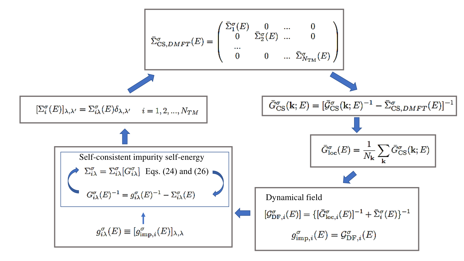
II.3 DMFT approximation
The self-energy of the CS, , is a matrix, which is energy- and momentum-dependent like the retarded CS Green’s function. The calculations accounting for both the - and the -dependence is a computationally too demanding task for realistic systems. Therefore, we employ the DMFT approximation to simplify the problem, and we consider electron correlation local in spaceKotliar et al. 2006; Held 2007. We assume the self-energy matrix to be momentum independent and to have block-diagonal form
| (19) |
where is the block for the orbitals of the TM atom . may in general be non-diagonal. The self-energy is evaluated via the self-consistent DMFT procedureKotliar et al. 2006; Held 2007. Our implementation is similar to that suggested by Valli et al. for model systems Valli et al. 2012 and Jacob et al. for nano-contacts Jacob et al. 2010. The main steps are the following:
- i)
We compute the dressed Green’s function in Eq. (14) with instead of . In the first iteration of the self-consistent procedure we need an initial guess for the . In our calculation we set it to zero.
- ii)
We define the so-called local Green’s function
(20) - iii)
We build the dynamical field for each TM atom inside the CS
(21) where is the block of the local Green’s function matrix relative to the atom .
- iv)
We map each of the atom inside the CS into an impurity model by defining the bare impurity Green’s function of each TM atom as .
- v)
We solve the impurity problems as described in the next section and we get the impurity self-energies for each atom .
- vi)
We set for each atom and recompute the CS DMFT self-energy in Eq. (19).
These steps are iterated to convergence.
Once the self-energy is computed, the self-energy matrix of the whole surface region is obtained and transformed into the original basis set . We note that in spite of the DMFT approximation used to compute the CS self-energy, the self-energy of the surface region in the original basis acquires a -dependence because of the transformation matrices in Eq. (16).
II.4 Self-energy in perturbation theory
We now describe in detail the method used to compute the self-energy by solving the impurity problem. In case of weakly or moderately correlated systems, such as the ferromagnetic metals of interest here, the self-energy can be obtained using self-consistent perturbative approaches in terms of skeleton diagrams around the non-interacting solution. A popular scheme is the self-consistent fluctuating exchange approximation (FLEX) Bickers and Scalapino 1989, which is conserving in the Baym-Kadanoff sense Baym and Kadanoff 1961; Baym 1962; Stefanucci and van Leeuwen 2013.
The FLEX has been further combined with the -matrix approximation, into the spin-polarized -matrix fluctuating exchange approximation Lichtenstein and Katsnelson 1998; Katsnelson and Lichtenstein 1999; Katsnelson and Lichtenstein 2002; Pourovskii et al. 2006, the so-called SPT-FLEX impurity solver.
The SPT-FLEX self-energy is described by the Hartree and Fock diagrams with the formal replacement of the bare interaction by the -matrix Galitski 1958; Kanamori 1963, which obeys the Bethe-Salpether-like integral equation.
The SPT-FLEX is formulated on the imaginary (Matsubara) frequency axis and correlation functions are obtained indirectly via the numerical analytical continuation to the real frequency axis.
Unfortunately, this often leads to numerical difficulties since the analytical continuation of discrete numerical data is not unambiguous and, in addition, it requires the treatment of the high-frequency “tails” Serene and Hess 1991. For this reason, we consider here a simpler second order perturbative treatment implemented to provide the self-energy directly on the real frequency axis, while retaining the multi-orbital nature of the many-body problem. A similar approach was used by Drchal et al. to study TM alloysDrchal et al. 1999. The method represents a good compromise between the need for an accurate description of correlated effects and for a efficient and easy numerical evaluation of spectral properties.
We assume that the matrix for the impurity problem associated to the TM atom in Eq. (21) is diagonal. This greatly reduces the computational effort of the calculations. We denote the diagonal elements of the impurity bare Green’s function and self-energy as and , where labels the orbitals. The Dyson equation for the impurity problem is then
| (22) |
where is the dressed Green’s function for orbital of the the impurity . The self-energy up to the second order in perturbation theory in over the band width is obtained by using the skeleton diagrams in appendix A, and is written as
| (23) |
The first-order contribution
| (24) |
is the well-known Hartree-Fock approximation, where
| (25) |
is the occupation of the orbital of spin at the atom ; is the Fermi function.
is local in time, i.e. energy independent. It therefore represents a one-electron potential producing only a shift of the non-interacting energy levels.
The second order contribution can be split into its real and imaginary part. The imaginary part is given by
| (26) | |||||
where
| (27) |
is the spectral function of . The real part is given by the Kramers-Kronig relations
| (28) |
Eqs. (26) and (28) are easily implemented thus allowing for the calculation of the second order self-energy contributions.
The approximation for the self-energy that we introduced is called second Born-approximation Stefanucci and van Leeuwen 2013 and it is conserving in the Baym-Kadanoff sense. Eq. (22) needs to be solved self-consistently together with Eqs. (24) and (26) because the self-energy is a functional of the dressed impurity Green’s function, that is and .
Eqs. (26) and (28) are easily implemented thus allowing for the calculation of the second order self-energy contributions.
The numerical integration over the frequencies and in Eq. (26) would potentially represent a computational bottleneck of the method if it was carried out using a too large number of discrete frequency points.
However, in the case of ferromagnetic TMs, we find accurate results already for relatively coarse energy grids ( eV) thus making the evaluation of computationally quite inexpensive.
II.5 Self-energy calculations combined with DFT
We now discuss how self-energy calculations are combined with DFT, and how the first and second order contributions are taken into account in our numerical implementation. Different scheme are proposed to carry out calculations.
II.5.1 The reduction to LSDA+U
The first order term of Eq. (23) combined with DFT reduces to the LSDA+U approach. The double counting correction of Eq. (11) can be englobed into and can be approximated with one of the various forms proposed for LSDA+U Himmetoglu et al. 2014. For example, using the so-called fully-localized limit Czyżyk and Sawatzky 1994 for , leads to
| (29) |
where is the total occupation, and and are the average effective Coulomb and exchange interactions in Eqs. (12) and (13). is exactly the Hubbard corrective potential of the LSDA+U Hamiltonian proposed by Lichtenstein et al. in Ref. Liechtenstein et al. 1995 [note that, differently from the original formulation, only diagonal elements of the density matrix appear in Eq. (29) because we assumed the Green’s function to be diagonal in the orbital indices]. Based on these observations, we evaluate the first-order self-energy performing a standard LSDA+U calculation. Although, Eq. (29) is the most complete formulation of the LSDA+U Hubbard corrective potential with fully orbital-dependent electronic interactions, we use a simplified expression introduced by Dudarev et al. Dudarev et al. 1998
| (30) |
to reduce the complexity of the calculations. This simplified expression has been successfully applied in several studies and for most materials it yields similar results as the fully rotationally invariant formulation (see Ref. Himmetoglu et al. 2014 and references therein for more details).
II.5.2 The LSDA+ scheme
The self-energy can be evaluated in terms of the bare impurity Green’s function instead of the dressed impurity Green’s function, i.e. and with that
replaces in Eqs. (25) and (27).
The approach has already been used in the literature Liebsch and Lichtenstein 2000, and in particular in Refs. Kleinman and Mednick 1981; Tréglia, G. et al. 1982; Aligia 2006, although these papers consider a single-orbital model Aligia 2006 or an average interaction (Ref. Tréglia, G. et al. 1982), while we maintain a multi-orbital description including the complete four-index interaction. The approximation using bare Green’s functions neglects some the diagrams in the perturbative expansion of the self-energy compared to the second Born-approximationStefanucci and van Leeuwen 2013 and it is non-conserving in the Baym-Kadanof sense. Nonetheless, we find that both approaches provide similar total number of electrons.
The fact that the Hartree-Fock self-energy is static leaves us the freedom to chose how to practically perform the perturbative calculations up to second order. Namely, starting from the non-interacting Green’s function we can calculate the total self-energy corrections up to second order, i.e. including the static and the dynamic
contributions. Alternatively, we can ”immerse” the static contribution, approximated as in Eq. (30), into the non-interacting local Green’s functions. This means that
is replaced by the LSDA+U Green’s function
| (31) |
The Dyson Eq. (22)
retains its structure with the total self-energy substituted by the correlation self-energy , where
is evaluated using the LSDA+U Green’s functions .
Following these considerations, our calculations are practically carried out in the following way.
We perform a fully charge self-consistent LSDA+U calculation and we obtain with the LSDA+U occupation of atom and orbital . Then, in the first DMFT iteration, we use as impurity Green’s function, which already contains the Hartree-Fock part of the self-energy, while we compute the second order self-energy corrections inserting into Eq. (26). The DMFT equations are eventually iterated solving the impurity problem by re-evaluating and at each DMFT iteration. For the systems of interest here, and in the limit of weak interactions, we found the DMFT self-consistent procedure converges very fast, and changes in the DOS are negligible after the first few DMFT iteration. In fact perturbative corrections in metallic systems lead to moderate changes of the electronic structure. The system remains a well defined Fermi liquid with modified parameters.
We refer to such computational approach as LSDA+. Calculations carried out by means LSDA+ add just a small computational cost to standard LSDA+U calculations, while already capturing some correlation effects as shown in Sec. IV.
II.5.3 Self-consistent approximation
The self-energy terms are evaluated as functionals of the dressed impurity Green’s function, that is and . A calculation requires in practice two self-consistent cycles as shown in Fig. 2. The first, is the DMFT cycle explained in Sec. II.3. Then at each DMFT iteration, a second self-consistent cycle is done to solve the impurity problem as explained in Sec. II.4. To ensure electron conservation inside the impurity according to the Luttinger-Ward theorem Stefanucci and van Leeuwen 2013, we add an identical on-site potential to all correlated orbitals and we readjust at each iteration.
III Computational details
We treat core electrons with norm-conserving Troullier-Martin pseudopotentials.
The valence states are expanded through a numerical atomic orbital basis set including multiple- and polarized functions Soler et al. 2002.
The electronic temperature is set to K.
The real space mesh is set by an equivalent energy cutoff of Ry. We use -point mesh to compute the self-consistent charge density with LSDA(+U).
This charge density is then used as input in a non-self-consistent calculation
to obtain the density of states employing -points. We shift all energies in such a way to set the Fermi level at 0 eV.
To calculate the second-order self-energy, we use a frequency grid comprising 4400 points and extending from to eV. The imaginary part in Eq. (3) is 0.01 eV and 0.005 eV in LSDA(+U) and in LSDA+
calculations, respectively. This leads to an additional broadening of the DOS for a better display in Figs. 3 and 4.
We express the Coulomb parameters in terms of Slater integrals , and (Ref. Imada et al. 1998).
These are connected to the average effective Coulomb and exchange interactions of Eqs. (12) and (13) through the relations and
. The ratio is assumed to correspond to the atomic value Anisimov and Gunnarsson 1991.
IV Electronic structure of Fe/W(110)
To describe the performances of our method we consider a monolayer of Fe on a W(110) substrate, a systems quite investigated in nanoscale magnetism and often used in spin-polarized scanning tunneling experiments Kubetzka et al. 2002; Samarin et al. 2013. The system is presented in Fig. 1. Only the results of spin-polarized calculations in the ferromagnetic phase are described, while non-magnetic calculations are shown in Appendix B. We remark that our method treats the W substrate as truly semi-infinite. This is an advantage compared to standard implementations of DFT and DFT+DMFT, where Fe/W(110) would be described as a slab with few W layers and therefore introducing unwanted confinement effects in the system electronic structure.
IV.1 Density of states
The Fe DOS calculated by means of LSDA, LSDA+U and LSDA+ is presented in Fig. 3. By analysing the results of the different methods we will understand the effect of the dynamical self-energy compared to mean-field static approximations.
To begin with, we observe that already the DOS obtained by using LSDA(+U) has an intrinsic broadening in our calculations. This is due to the embedding matrix function between the surface region and the W bulk continuum states in Eq. (3). The effect would be absent in calculations considering a slab geometry for Fe/W(110), and it demonstrates the importance of using our implementation of DFT to accurately describe surfaces and interfaces.
The LSDA results are shown in Fig. 3-a. The spin up (majority) and spin down (minority) DOS are split by about 2 eV (Fig. 3-a). Comparing with the orbital resolved DOS in Fig. 4, we find that the prominent peaks for both spin channels have mostly character.
The total DOS for the spin up channel is centered at eV and is almost completely filled. The total occupation of the
majority orbitals
is 4.68 electrons.
In contrast, the spin down DOS presents two main peaks at the opposite sides of the Fermi level and separated by a pseudo-gap.
As seen in the orbital-resolved DOS in Fig. 4, the two-peak structure reflects the separation of the Fe and from the , and orbitals due to the (110) surface symmetry.
The orbitals are oriented along the crystal direction connecting the surface Fe atoms and thus merge into bonding and anti-bonding bands.
The Fe orbitals overlap with the orbitals of the W atoms underneath forming a second set of bonding and anti-bonding bands.
All bonding states are centered at about eV giving the first sharp peak in the spin down DOS, while the antibonding states are unoccupied and emerge as very broad features extending up to eV.
The , and orbitals mostly overlap with orbitals forming broad states centered around eV. They contribute to the second unoccupied peak in the spin down DOS.
The occupation of the Fe and orbitals is about , whereas that of the , and orbitals is , contributing to the total occupation of the minority states equal to electrons.
The spin magnetic moment is , considerably enhanced with respect to that in bulk Fe, 2.2 .
The DOS calculated by means of LSDA+U is shown in Fig. 3-c and -e for eV and eV, respectively, and eV.
In such a mean-field like approach the potential shifts the spin up LSDA DOS towards lower energies by about [see Eq. (30)].
The occupation of the spin up states therefore increases as a function of .
In contrast, the potential barely affects the spin down and orbitals, and moves the , and orbitals towards higher energies by about .
The pseudo-gap in the spin down DOS across the Fermi level widens, while the
, and orbitals are slightly emptied. Overall, the splitting between the spin up and down DOS becomes larger
and, as a result, the total Fe magnetic moment systematically increases as a function of .
This is a general outcome of DFT+U calculations found for all ferromagnetic materials Cococcioni and de Gironcoli 2005.
It is a consequence of the fact that the potential of Eqs. (29) and (30) represents the Hartree-Fock approximation to the Hubbard interaction.
Next, we discuss the results obtained including second order self-energy contributions via the approach described in Sec. II.5.2. The DOS are shown in Fig. 3-b, -d and -f. We use eV and eV and eV like in the LSDA+U calculations.
Since the LSDA bandwidth is about 4.5 eV, the perturbation expansion is valid.
We note that the Fe atoms Green’s function is not diagonal. However the off-diagonal elements are typically two orders of magnitude smaller than diagonal elements. They can therefore be discarded, consistent with our assumption in Sec. II.4.
The calculations in Fig. 3-b, which are indicated as “LSDA+ (no HF)”, are carried out neglecting the approximate Hartree-Fock potential of Eq. (30) and using the LSDA Green’s function to evaluate second order self-energy contributions.
The main features due to the second order self-energy are similar across Fig. 3-b, -d and -f. Some redistribution of the spectral weight occurs resulting in a considerable spectral narrowing.
The orbital ordering (orbitals’ position in energy) and the character of the main peaks recognizable in Fig. 4 is preserved as it is dictated by the surface symmetry and the crystal field.
The changes in the DOS are more pronounced for spin up than for spin down. The top of the occupied DOS
in the spin up channel is shifted towards the Fermi level, while the down DOS is barely affected.
This leads to a lowering of the Fe magnetic moment reported in Tab. 1.
For eV, we observe a reduction in excess of compared to LSDA+U thus
demonstrating that correlation effects play a crucial role in counterbalancing the exchange interaction. This can be easily understood by inspecting the mathematical form of the second order self-energy of Eq. (26)
or the corresponding Feynman diagrams in the appendix.
Electronic correlations are build-up by the scattering processes between electrons and electron-hole pairs.
Since the spin up channel is essentially full, electron-hole pairs are mostly created in the spin down channel.
Therefore a spin up electron will more likely scatter with an opposite-spin pair costing an effective interaction .
In contrast, a spin down electron will scatter with same-spin pairs with effective interaction .
Therefore, correlation effects are stronger for spin up than for spin down electrons.
| Method | |||
|---|---|---|---|
| LSDA | 4.68 | 1.85 | 2.84 |
| LSDA+ (no HF) | 4.57 | 1.96 | 2.6 |
| LSDA+U ( eV) | 4.75 | 1.75 | 3.0 |
| LSDA+ ( eV) | 4.69 | 1.81 | 2.88 |
| LSDA+U ( eV) | 4.79 | 1.69 | 3.1 |
| LSDA+ ( eV) | 4.65 | 1.88 | 2.76 |
Analyzing in more details the results for eV, we note that the spin up DOS center is predicted at eV and at eV respectively in calculations without and with the HF potential (Fig. 3-b and 3-d). Clearly the differences in the two cases are due to the initial state dependence of perturbation theory and they reflect the differences between the LSDA and LSDA+U DOS. In spite of that, the two results are overall quite similar.
In this specific case, neglecting the HF potential and using the LSDA Green’s function to compute is a practical and reliable simplification.
Next, w compare the LSDA+ results for eV and for eV (Fig. 3-d and -f respectively). We see that a larger does not significantly change the position of the states, but it induces a narrowing of both the spin up and the spin down DOS features.
According to this finding, an increase in the local Coulomb parameter including dynamic self-energy effects leads to a re-shaping of the spectrum rather than in a modification of their spin-splitting as one would expect based on a static mean-field picture.
For energies far below from the Fermi level, we distinguish a satellite appearing in the spin-up channel below -4 eV.
A similar feature has been unequivocally observed in photoemission measurements for Ni Guillot et al. 1977 and it has been predicted for bulk Fe as well Grechnev et al. 2007. Here we predict that it is present even in a Fe monolayer. As already noted in Ref. Grechnev et al. 2007 for bulk calculations, albeit performed with a SPT-FLEX impurity solver instead of , the center of the satellite systematically shifts towards lower energies when increasing .
Finally, we present the results of calculations, referred to as LSDA+sc, where the self-energy is evaluated self-consistently as explained in Sec. II.5.3.The DOS is shown in Fig. 5 for and eV ( eV in both cases). The self-consistent iterations lead to a redistribution of the spin up spectral weight, in particular at energies far from the Fermi level. The spin down DOS remains almost unaltered owing to the low correlation. For eV, the spin-splitting of the states remains equal to that predicted in the LSDA+ calculations. In contrast, for eV, the spin up states are moved towards the Fermi energy by about 0.2 eV compared to non-self-consistent calculations. Thus, the DOS spin-splitting is reduced. Overall, we find that the self-consistent procedure mitigates the initial state dependence of perturbation theory, although it does not completely eliminate it. Notably, at energies far below the Fermi level, the satellite feature becomes much less marked in the LSDA+sc than in LSDA+ DOS. The self-consistent calculation enhances multi-band screening effects thus leading to a partial suppression of that intrinsic many-body feature.
IV.2 Self-energy and effective masses
The changes in the DOS induced by the dynamical correlation effects can be understood by inspecting the self-energy, which is presented in Fig. 6 for different cases.
Since the crystal-field splitting is rather small, the self-energy is very similar for all orbitals. Thus, we present in Fig. 6 the self-energy averaged over the orbital indexes.
The overall shape of the real and imaginary parts is typical of ferromagnetic transition metals Grechnev et al. 2007.
For example, in Fig. 6-a we note that,
in the spin up channel, the real part of the self-energy is positive in the energy range between eV and the Fermi level, and it shows a maximum at about eV.
This causes the shift of occupied states
towards to the Fermi level as observed in Fig. 3. In contrast, for energies below eV, the negative real part of the self-energy draws the spectral weight towards lower energies
leading to the formation of the satellite in the DOS. The imaginary part has an extended negative peak centered at eV resulting in the large broadening of the satellite. Increasing the value to eV (Fig. 6-c),
the peak in the real part of the self-energy for spin up is enhanced to compensate the larger LSDA+U potential,
which brings the spin up states towards too low energies. The maximum of the imaginary part also becomes more pronounced than for eV.
In the spin down channel, correlation effects are much less pronounced for both and eV and the self-energy is quite small.
It is interesting to observe how the spin up self-energy changes when evaluated self-consistently (Fig. 6-b). The positive maximum of the real part shifts of almost 2 eV towards the Fermi energy compared to the non-self-consistent LSDA+ calculation. Furthermore, in the energy region below eV, where the real part of the self-energy is negative, its magnitude is reduced. Similarly, the imaginary part also becomes smaller. These two factors explain why the satellite is partly suppressed in self-consistent self-energy calculations.
The self-energy near the Fermi level has Fermi-liquid character: for the imaginary part, we have , whereas the real part has negative slope, . We then evaluate the mass enhancement, which amounts to
| (32) |
where represents the band-mass obtained within the LSDA(+U) calculations. The enhancement factors with respect to LSDA are very similar for all orbitals and spin channels. For eV, they are on average about , which indicates that the system is medium-correlated. When the self-energy is calculated self-consistently, becomes larger and is equal to about . This is a due of the shift of the main peak of towards the Fermi level. Therefore we find that, while the self-consistent iterations partly suppresses many-body correlation effects at high energy, they make electrons at the Fermi energy slightly more correlated.
IV.3 Comparison to experimental data
We now assess the performances of the various methods against experiments. Photoemission spectra of a Fe monolayer on W(110) were measured in Ref. Getzlaff et al. 1997 with the electron excitation occurring along the -- direction of the Brillouin zone. The results are presented as small triangles in Fig. 7 along with the DOS calculated by using LSDA, LSDA+, LSDA+sc for eV and eV. Since electrons from both Fe and W contribute to the experimental signal, we present the sum of the DOS of the Fe monolayer and of the first W layer underneath. The DOS is convoluted with a Fermi function to introduce a smooth cut-off around the Fermi energy. We assume that the DOS can be directly compared to experiments, which means that transition matrix element effects are neglected.
The most striking observation is that LSDA drastically overestimates the spin-splitting between majority and minority states. The experimental spin up spectrum quickly rises below the Fermi energy and the maximum is at eV, whereas the LSDA DOS for the spin up channel is centered at about eV. The inability of LSDA to accurately predict the spin-splitting of states in metallic ferromagnetic systems has been pointed out in a number of works Monastra et al. 2002; Braun et al. 2006; Grechnev et al. 2007.
Calculations including dynamical self-energy contributions shift the majority DOS towards the Fermi level thus correcting for the LSDA short-comes. The LSDA+ DOS is in quantitative agreement with the experimental data. The method captures the main correlation effect in the system.
We can not identify which scheme, LSDA+ or LSDA+sc, performs better. Both methods give a very similar DOS in the energy range, where the experimental data is available, and the broadening of the photoemission spectrum does not allow to distinguish between small differences in the spectral distribution. Photoemission experiments probing the the energy region eV and the existence of the satellite features would provide stronger indications about the accuracy of LSDA+ and LSDA+sc. We hope that these experiments will be performed in the future.
V Conclusions
DFT+ combines DFT to a multi-orbital solver for the Hubbard model, where the Coulomb interaction parameter is treated in perturbation theory up to second order. The method provides a realistic description of moderately correlated materials. Our implementation is designed to investigate TM surfaces, interfaces, and layered systems in general.
As an example of application, we considered a Fe monolayer on a W(110) substrate. We discussed in detail the correlated DOS comparing the results with those of LSDA and LSDA+U calculations.
We found that second order self-energy contributions led to a shift of the majority-spin DOS towards the Fermi level and therefore to a reduction of the states spin-splitting compared to LSDA calculations. This result is in quantitative agreement with available photoemission spectra.
The use of different unperturbed states and the inclusion of the first-order contribution in DFT+ gave differences in the DOS spin-splitting and spectral width.
These differences were nonetheless rather minor. The self-consistent evaluation of the self-energy
leads to a redistribution of the spin up spectral weight,
in particular at energies far from the Fermi level. The spin-splitting of the states changes very little during the self-consistent cycle. In contrast, a satellite feature far in energy below the Fermi level is considerably reduced owing to multi-band screening effects.
In our calculations we employed the local approximation thus we neglected spatially non-local correlation effects. However, the calculation of second order self-energy contribution can in principle be extended to allow for momentum dependence, although this would increase significantly the complexity of the numerical implementation and the computational overhead.
Overall, our implementation of DFT+ can be readily used to simulate, at a relatively low computational cost, correlation effects in the electronic structure of heterostructures comprising TMs. The calculation of the self-energy on the real energy axis is particularly convenient if one is interested in treating charge and spin transport properties using generalized Landauer methods Droghetti and Rungger 2017; Jacob 2015, which require the evaluation of the energy dependent transmission function Chioncel et al. 2015; Rungger et al. 2019. As such, we believe that DFT+ will provide important theoretical inputs for the design of materials and devices for electronics and spintronics.
VI Acknowledgements
AD and AH acknowledge funding by the Science Foundation Ireland (SFI) and the Royal Society through the University Research Fellowship URF-R1-191769. MMR acknowledges funding provided by the Institute of Physics Belgrade, through the grant by the Ministry of Education, Science, and Technological Development of the Republic of Serbia. IR acknowledges the support of the UK government department for Business, Energy and Industrial Strategy through the UK national quantum technologies programme. LC acknowledges the financial support by the Deutsche Forschungsgemeinschaft through TRR80 (project F6) Project number 107745057. Computational resources were provided by Trinity College Dublin Research IT.
Appendix A Second order self-energy
We provide here details about the perturbative treatment of the multi-orbital electronic system. We use the Keldysh Green’s functions formalism Stefanucci and van Leeuwen 2013. The self-energy, up to second order can be schematically expressed using skeleton Feynman diagrams
where the dots represents space-(contour time) coordinates, the straight line represents the dressed Green’s function and the wiggly lines represents the interaction. Converted into equations these diagrams give four contributions to the self-energy
| (49) | |||
| (50) | |||
| (51) | |||
In the specific case of the Hubbard model, the interaction matrix is time and momentum independent and we refer to it as in the main text. Additionally, the Hubbard matrix is also spin independent, but, in this appendix, we keep the spin indices in accordance with the most general notation.
After applying the Langreth rules Stefanucci and van Leeuwen 2013 and performing the Fourier transform we obtain the first order terms
where the lesser Green’s function in equilibrium assumes the following form
| (54) |
with the retarded Green’s function and the Fermi function. The first order terms
can then be written in well known Hartree-Fock expression
of Eq. (24).
The two second order terms giving reads
| (55) |
| (56) |
After a few steps of algebra and neglecting the momentum dependence, we easily obtain Eq. (26). We note that we drop the superscript “” for “retarded” in the main text to keep the notation lighter.
Appendix B Non-magnetic calculations
Self-energy calculations can be carried out also for the non-magnetic phase and can be combined with DFT within the local density approximation (LDA).
The non-magnetic orbital-resolved DOS obtained with LDA and LDA+ is presented in Fig. 8.
The general features are similar to those discussed in Sec. IV.1. In LDA calculations, the DOS extends across the Fermi energy from about eV to eV, i.e. over the band width equal to about eV. There are two peaks well below the Fermi energy, at eV and eV. They stem respectively from the and orbitals. Instead, the and orbitals give the dominant contribution to quite sharp peaks at the Fermi energy. The DOS projected over is much smoother. Overall the total DOS at the Fermi energy is eV-1. Using the Stoner parameter eV estimated from the band-splitting in Fig. IV.1 as explained in Refs. Gunnarsson 1978; Zeller 2006, the Stoner criterion is satisfied and therefore the ferromagnetic state is favored over the non-magnetic one. The same conclusion is also found by comparing the DFT total energies of the two states.
The orbital has the largest occupation equal to about electrons, while and have the lowest occupation, respectively and electrons. The orbitals and orbital have similar occupations of about electrons.
The second order self-energy induces some redistribution of the spectral weight. The main effect in LDA+ is that the peaks associated to the and orbitals in the DOS at the Fermi level become sharper, while the other peaks stemming from and are shifted towards by about eV. Furthermore, the satellite at eV appears.
In self-consistent self-energy calculations, some further spectral redistribution occurs. The peak in the -projected DOS (blue line) at about eV gets reshaped into a shoulder-like feature accompanying the main peak at . At the same time, the peak in the -projected DOS (green line) becomes broader. As, found for the spin-polarized calculation, the satellite becomes much less marked.
References
- Tusche et al. (2018) C. Tusche, M. Ellguth, V. Feyer, A. Krasyuk, C. Wiemann, J. Henk, C. M. Schneider, and J. Kirschner, Nat. Commun. 9, 3727 (2018), URL https://doi.org/10.1038/s41467-018-05960-5.
- Wiesendanger (2009) R. Wiesendanger, Rev. Mod. Phys. 81, 1495 (2009), URL https://link.aps.org/doi/10.1103/RevModPhys.81.1495.
- Jones and Gunnarsson (1989) R. O. Jones and O. Gunnarsson, Rev. Mod. Phys. 61, 689 (1989), URL http://link.aps.org/doi/10.1103/RevModPhys.61.689.
- Kohn (1999) W. Kohn, Rev. Mod. Phys. 71, 1253 (1999).
- Jones (2015) R. O. Jones, Rev. Mod. Phys. 87, 897 (2015), URL http://link.aps.org/doi/10.1103/RevModPhys.87.897.
- von Barth and Hedin (1972) U. von Barth and L. Hedin, J. Phys. C 5, 1629 (1972).
- Vosko et al. (1980) S. H. Vosko, L. Wilk, and M. Nusair, Can. J. Phys. 58, 1200 (1980).
- Perdew et al. (1992) J. P. Perdew, J. A. Chevary, S. H. Vosko, K. A. Jackson, M. R. Pederson, D. J. Singh, and C. Fiolhais, Phys. Rev. B 46, 6671 (1992), URL https://link.aps.org/doi/10.1103/PhysRevB.46.6671.
- Perdew et al. (1993) J. P. Perdew, J. A. Chevary, S. H. Vosko, K. A. Jackson, M. R. Pederson, D. J. Singh, and C. Fiolhais, Phys. Rev. B 48, 4978 (1993), URL https://link.aps.org/doi/10.1103/PhysRevB.48.4978.2.
- Perdew et al. (1996) J. P. Perdew, K. Burke, and M. Ernzerhof, Phys. Rev. Lett. 77, 3865 (1996), URL https://link.aps.org/doi/10.1103/PhysRevLett.77.3865.
- Monastra et al. (2002) S. Monastra, F. Manghi, C. A. Rozzi, C. Arcangeli, E. Wetli, H.-J. Neff, T. Greber, and J. Osterwalder, Phys. Rev. Lett. 88, 236402 (2002), URL https://link.aps.org/doi/10.1103/PhysRevLett.88.236402.
- Braun et al. (2006) J. Braun, J. Minár, H. Ebert, M. I. Katsnelson, and A. I. Lichtenstein, Phys. Rev. Lett. 97, 227601 (2006), URL https://link.aps.org/doi/10.1103/PhysRevLett.97.227601.
- Guillot et al. (1977) C. Guillot, Y. Ballu, J. Paigné, J. Lecante, K. P. Jain, P. Thiry, R. Pinchaux, Y. Pétroff, and L. M. Falicov, Phys. Rev. Lett. 39, 1632 (1977), URL https://link.aps.org/doi/10.1103/PhysRevLett.39.1632.
- Imada et al. (1998) M. Imada, A. Fujimori, and Y. Tokura, Rev. Mod. Phys. 70, 1039 (1998).
- Anisimov et al. (1991) V. I. Anisimov, J. Zaanen, and O. K. Andersen, Phys. Rev. B 44, 943 (1991), URL https://link.aps.org/doi/10.1103/PhysRevB.44.943.
- Liechtenstein et al. (1995) A. I. Liechtenstein, V. I. Anisimov, and J. Zaanen, Phys. Rev. B 52, R5467 (1995), URL https://link.aps.org/doi/10.1103/PhysRevB.52.R5467.
- Dudarev et al. (1998) S. L. Dudarev, G. A. Botton, S. Y. Savrasov, C. J. Humphreys, and A. P. Sutton, Phys. Rev. B 57, 1505 (1998), URL https://link.aps.org/doi/10.1103/PhysRevB.57.1505.
- Cococcioni and de Gironcoli (2005) M. Cococcioni and S. de Gironcoli, Phys. Rev. B 71, 035105 (2005), URL https://link.aps.org/doi/10.1103/PhysRevB.71.035105.
- Metzner and Vollhardt (1989) W. Metzner and D. Vollhardt, Phys. Rev. Lett. 62, 324 (1989).
- Georges et al. (1996) A. Georges, G. Kotliar, W. Krauth, and M. J. Rozenberg, Rev. Mod. Phys. 68, 13 (1996).
- Kotliar and Vollhardt (2004) G. Kotliar and D. Vollhardt, Phys. Today 57, 53 (2004).
- Kotliar et al. (2006) G. Kotliar, S. Y. Savrasov, K. Haule, V. S. Oudovenko, O. Parcollet, and C. A. Marianetti, Rev. Mod. Phys. 78, 865 (2006).
- Held (2007) K. Held, Adv. Phys. 56, 829 (2007).
- Lichtenstein et al. (2001) A. I. Lichtenstein, M. I. Katsnelson, and G. Kotliar, Phys. Rev. Lett. 87, 067205 (2001).
- Grechnev et al. (2007) A. Grechnev, I. Di Marco, M. I. Katsnelson, A. I. Lichtenstein, J. M. Wills, and O. Eriksson, Phys. Rev. B 76, 035107 (2007), URL https://link.aps.org/doi/10.1103/PhysRevB.76.035107.
- Östlin et al. (2018) A. Östlin, L. Vitos, and L. Chioncel, Phys. Rev. B 98, 235135 (2018), URL https://link.aps.org/doi/10.1103/PhysRevB.98.235135.
- Katsnelson et al. (2008) M. I. Katsnelson, V. Y. Irkhin, L. Chioncel, A. I. Lichtenstein, and R. A. de Groot, Rev. Mod. Phys. 80, 315 (2008), URL https://link.aps.org/doi/10.1103/RevModPhys.80.315.
- Beiuşeanu et al. (2011) F. Beiuşeanu, C. Horea, E.-V. Macocian, T. Jurcuţ, L. Vitos, and L. Chioncel, Phys. Rev. B 83, 125107 (2011), URL https://link.aps.org/doi/10.1103/PhysRevB.83.125107.
- Chioncel et al. (2011) L. Chioncel, I. Leonov, H. Allmaier, F. Beiuşeanu, E. Arrigoni, T. Jurcuţ, and W. Pötz, Phys. Rev. B 83, 035307 (2011), URL https://link.aps.org/doi/10.1103/PhysRevB.83.035307.
- Di Marco et al. (2018) I. Di Marco, A. Held, S. Keshavarz, Y. O. Kvashnin, and L. Chioncel, Phys. Rev. B 97, 035105 (2018), URL https://link.aps.org/doi/10.1103/PhysRevB.97.035105.
- Keshavarz et al. (2020) S. Keshavarz, I. Di Marco, D. Thonig, L. Chioncel, O. Eriksson, and Y. O. Kvashnin, Phys. Rev. Materials 4, 021401 (2020), URL https://link.aps.org/doi/10.1103/PhysRevMaterials.4.021401.
- Chioncel et al. (2005) L. Chioncel, M. I. Katsnelson, G. A. de Wijs, R. A. de Groot, and A. I. Lichtenstein, Phys. Rev. B 71, 085111 (2005), URL https://link.aps.org/doi/10.1103/PhysRevB.71.085111.
- Chioncel et al. (2015) L. Chioncel, C. Morari, A. Östlin, W. H. Appelt, A. Droghetti, M. M. Radonjić, I. Rungger, L. Vitos, U. Eckern, and A. V. Postnikov, Phys. Rev. B 92, 054431 (2015), URL https://link.aps.org/doi/10.1103/PhysRevB.92.054431.
- Morari et al. (2017) C. Morari, W. H. Appelt, A. Östlin, A. Prinz-Zwick, U. Schwingenschlögl, U. Eckern, and L. Chioncel, Phys. Rev. B 96, 205137 (2017), URL https://link.aps.org/doi/10.1103/PhysRevB.96.205137.
- Lichtenstein and Katsnelson (1998) A. I. Lichtenstein and M. I. Katsnelson, Phys. Rev. B 57, 6884 (1998), URL https://link.aps.org/doi/10.1103/PhysRevB.57.6884.
- Katsnelson and Lichtenstein (1999) M. I. Katsnelson and A. I. Lichtenstein, J. Phys.: Condens. Matter 11, 1037 (1999).
- Katsnelson and Lichtenstein (2002) M. I. Katsnelson and A. I. Lichtenstein, Eur. Phys. J. B 30, 9 (2002).
- Pourovskii et al. (2006) L. V. Pourovskii, M. I. Katsnelson, and A. I. Lichtenstein, Phys. Rev. B 73, 060506 (2006), URL https://link.aps.org/doi/10.1103/PhysRevB.73.060506.
- Jarrell and Gubernatis (1996) M. Jarrell and J. Gubernatis, Physics Reports 269, 133 (1996), ISSN 0370-1573, URL https://www.sciencedirect.com/science/article/pii/0370157395000747.
- Sandvik (1998) A. W. Sandvik, Phys. Rev. B 57, 10287 (1998), URL https://link.aps.org/doi/10.1103/PhysRevB.57.10287.
- Beach et al. (2000) K. S. D. Beach, R. J. Gooding, and F. Marsiglio, Phys. Rev. B 61, 5147 (2000), URL https://link.aps.org/doi/10.1103/PhysRevB.61.5147.
- Jacob (2015) D. Jacob, Journal of Physics: Condensed Matter 27, 245606 (2015), URL https://doi.org/10.1088/0953-8984/27/24/245606.
- Droghetti and Rungger (2017) A. Droghetti and I. Rungger, Phys. Rev. B 95, 085131 (2017), URL https://link.aps.org/doi/10.1103/PhysRevB.95.085131.
- Rungger et al. (2019) I. Rungger, A. Droghetti, and M. Stamenova, in Handbook of Materials Modeling. Vol. 1 Methods: Theory and Modeling, edited by S. Yip and W. W. Andreoni (Springer International Publishing, 2019).
- Kubetzka et al. (2002) A. Kubetzka, M. Bode, O. Pietzsch, and R. Wiesendanger, Phys. Rev. Lett. 88, 057201 (2002), URL https://link.aps.org/doi/10.1103/PhysRevLett.88.057201.
- Samarin et al. (2013) S. Samarin, O. Artamonov, P. Guagliardo, K. Sudarshan, M. Kostylev, L. Pravica, A. Baraban, and J. Williams, Surface Science 617, 22 (2013), ISSN 0039-6028, URL https://www.sciencedirect.com/science/article/pii/S0039602813002185.
- Rocha et al. (2006) A. R. Rocha, V. M. García-Suárez, S. Bailey, C. Lambert, J. Ferrer, and S. Sanvito, Phys. Rev. B 73, 085414 (2006), URL https://link.aps.org/doi/10.1103/PhysRevB.73.085414.
- Soler et al. (2002) J. M. Soler, E. Artacho, J. D. Gale, A. García, J. Junquera, P. Ordejón, and D. Sánchez-Portal, Journal of Physics: Condensed Matter 14, 2745 (2002), URL https://doi.org/10.1088/0953-8984/14/11/302.
- Szabo and Ostlund (1996) A. Szabo and N. S. Ostlund, Modern Quantum Chemistry: Introduction to Advanced Electronic Structure Theory (Dover Publications Inc., Mineola NY, 1996).
- Brandbyge et al. (2002) M. Brandbyge, J.-L. Mozos, P. Ordejón, J. Taylor, and K. Stokbro, Phys. Rev. B 65, 165401 (2002), URL https://link.aps.org/doi/10.1103/PhysRevB.65.165401.
- Evers et al. (2004) F. Evers, F. Weigend, and M. Koentopp, Phys. Rev. B 69, 235411 (2004), URL https://link.aps.org/doi/10.1103/PhysRevB.69.235411.
- Palacios et al. (2002) J. J. Palacios, A. J. Pérez-Jiménez, E. Louis, E. SanFabián, and J. A. Vergés, Phys. Rev. B 66, 035322 (2002), URL https://link.aps.org/doi/10.1103/PhysRevB.66.035322.
- Kudrnovský et al. (1992) J. Kudrnovský, I. Turek, V. Drchal, P. Weinberger, N. E. Christensen, and S. K. Bose, Phys. Rev. B 46, 4222 (1992), URL https://link.aps.org/doi/10.1103/PhysRevB.46.4222.
- Nardelli (1999) M. B. Nardelli, Phys. Rev. B 60, 7828 (1999), URL https://link.aps.org/doi/10.1103/PhysRevB.60.7828.
- Taylor et al. (2001) J. Taylor, H. Guo, and J. Wang, Phys. Rev. B 63, 245407 (2001), URL https://link.aps.org/doi/10.1103/PhysRevB.63.245407.
- Sanvito et al. (1999) S. Sanvito, C. J. Lambert, J. H. Jefferson, and A. M. Bratkovsky, Phys. Rev. B 59, 11936 (1999), URL https://link.aps.org/doi/10.1103/PhysRevB.59.11936.
- Rungger and Sanvito (2008) I. Rungger and S. Sanvito, Phys. Rev. B 78, 035407 (2008), URL https://link.aps.org/doi/10.1103/PhysRevB.78.035407.
- Jacob et al. (2009) D. Jacob, K. Haule, and G. Kotliar, Phys. Rev. Lett. 103, 016803 (2009), URL https://link.aps.org/doi/10.1103/PhysRevLett.103.016803.
- Jacob et al. (2010) D. Jacob, K. Haule, and G. Kotliar, Phys. Rev. B 82, 195115 (2010), URL https://link.aps.org/doi/10.1103/PhysRevB.82.195115.
- Jacob and Kotliar (2010) D. Jacob and G. Kotliar, Phys. Rev. B 82, 085423 (2010), URL https://link.aps.org/doi/10.1103/PhysRevB.82.085423.
- Appelt et al. (2018) W. H. Appelt, A. Droghetti, L. Chioncel, M. M. Radonjić, E. Muñoz, S. Kirchner, D. Vollhardt, and I. Rungger, Nanoscale 10, 17738 (2018), URL http://dx.doi.org/10.1039/C8NR03991G.
- Pavarini (2011) E. Pavarini, in The LDA+DMFT approach to strongly correlated materials Modeling and Simulation Vol. 1, edited by E. Pavarini, E. Koch, D. Vollhardt, and A. Lichtenstein (Forschungszentrum Julich, 2011).
- Karolak et al. (2010) M. Karolak, G. Ulm, T. Wehling, V. Mazurenko, A. Poteryaev, and A. Lichtenstein, Journal of Electron Spectroscopy and Related Phenomena 181, 11 (2010), ISSN 0368-2048, URL https://www.sciencedirect.com/science/article/pii/S0368204810001222.
- Haule et al. (2010) K. Haule, C.-H. Yee, and K. Kim, Phys. Rev. B 81, 195107 (2010), URL https://link.aps.org/doi/10.1103/PhysRevB.81.195107.
- Valli et al. (2012) A. Valli, G. Sangiovanni, A. Toschi, and K. Held, Phys. Rev. B 86, 115418 (2012), URL https://link.aps.org/doi/10.1103/PhysRevB.86.115418.
- Bickers and Scalapino (1989) N. Bickers and D. Scalapino, Annals of Physics 193, 206 (1989), ISSN 0003-4916, URL https://www.sciencedirect.com/science/article/pii/000349168990359X.
- Baym and Kadanoff (1961) G. Baym and L. P. Kadanoff, Phys. Rev. 124, 287 (1961), URL https://link.aps.org/doi/10.1103/PhysRev.124.287.
- Baym (1962) G. Baym, Phys. Rev. 127, 1391 (1962), URL https://link.aps.org/doi/10.1103/PhysRev.127.1391.
- Stefanucci and van Leeuwen (2013) G. Stefanucci and R. van Leeuwen, Nonequilibrium Many-Body Theory of Quantum Systems: A Modern Introduction (Cambridge University Press, 2013).
- Galitski (1958) V. M. Galitski, Zh. Eksper. Teor. Fiz. 34, 1011 (1958).
- Kanamori (1963) J. Kanamori, Progress of Theoretical Physics 30, 275 (1963), ISSN 0033-068X, eprint https://academic.oup.com/ptp/article-pdf/30/3/275/5278869/30-3-275.pdf, URL https://doi.org/10.1143/PTP.30.275.
- Serene and Hess (1991) J. W. Serene and D. W. Hess, Phys. Rev. B 44, 3391 (1991), URL https://link.aps.org/doi/10.1103/PhysRevB.44.3391.
- Drchal et al. (1999) V. Drchal, V. Janiš, and J. Kudrnovský, Phys. Rev. B 60, 15664 (1999), URL https://link.aps.org/doi/10.1103/PhysRevB.60.15664.
- Himmetoglu et al. (2014) B. Himmetoglu, A. Floris, S. de Gironcoli, and M. Cococcioni, International Journal of Quantum Chemistry 114, 14 (2014), eprint https://onlinelibrary.wiley.com/doi/pdf/10.1002/qua.24521, URL https://onlinelibrary.wiley.com/doi/abs/10.1002/qua.24521.
- Czyżyk and Sawatzky (1994) M. T. Czyżyk and G. A. Sawatzky, Phys. Rev. B 49, 14211 (1994), URL https://link.aps.org/doi/10.1103/PhysRevB.49.14211.
- Liebsch and Lichtenstein (2000) A. Liebsch and A. Lichtenstein, Phys. Rev. Lett. 84, 1591 (2000), URL https://link.aps.org/doi/10.1103/PhysRevLett.84.1591.
- Kleinman and Mednick (1981) L. Kleinman and K. Mednick, Phys. Rev. B 24, 6880 (1981), URL https://link.aps.org/doi/10.1103/PhysRevB.24.6880.
- Tréglia, G. et al. (1982) Tréglia, G., Ducastelle, F., and Spanjaard, D., J. Phys. France 43, 341 (1982), URL https://doi.org/10.1051/jphys:01982004302034100.
- Aligia (2006) A. A. Aligia, Phys. Rev. B 74, 155125 (2006), URL https://link.aps.org/doi/10.1103/PhysRevB.74.155125.
- Anisimov and Gunnarsson (1991) V. I. Anisimov and O. Gunnarsson, Phys. Rev. B 43, 7570 (1991), URL https://link.aps.org/doi/10.1103/PhysRevB.43.7570.
- Getzlaff et al. (1997) M. Getzlaff, J. Bansmann, J. Braun, and G. Schönhense, Zeitschrift für Physik B Condensed Matter 104, 11 (1997).
- Gunnarsson (1978) O. Gunnarsson, Journal of Applied Physics 49, 1399 (1978), eprint https://doi.org/10.1063/1.325005, URL https://doi.org/10.1063/1.325005.
- Zeller (2006) R. Zeller, in Magnetism, in Computational Nanoscience: Do It Yourself!, edited by J. Grotendorst, S. Blügel, and D. Marx (NIC Serie, Forschungszentrum Julich, 2006), eprint http://juser.fz-juelich.de/record/54009/files/FZJ-2014-02225.pdf.