Symmetry-Protected Infinite-Temperature Quantum Memory from Subsystem Codes

We consider a square lattice with “gauge” qubits on its links $\ell$ and “matter” qubits on its vertices $v$ and on its plaquettes $p$ (see Fig. 1). The total Hilbert space is therefore $\bigotimes_{\ell,v,p}\mathbb{C}^{2}$. We refer to the full collection of gauge and matter qubits as “physical qubits,” to distinguish them from the logical qubit that is introduced later. Pauli operators for all physical qubits are denoted by $X_{r},Y_{r},Z_{r}$, with $r=\ell,v,p$ specifying the position of the qubit and

$\displaystyle X_{r}=\begin{bmatrix}0&1\\ 1&0\end{bmatrix}\,\,\,\,\,\,\,Y_{r}=\begin{bmatrix}0&-i\\ i&\,\,\,\,\,0\end{bmatrix}\,\,\,\,\,\,\,Z_{r}=\begin{bmatrix}1&\,\,\,\,\,0\\ 0&-1\end{bmatrix}.$

(1)

We employ boundary conditions on the square lattice inspired by the surface code Kitaev 2003; Bravyi and Kitaev 1998; Freedman and Meyer 2001; Fowler et al. 2012, taking “rough” boundaries with dangling links on the top and bottom and “smooth” boundaries without dangling links on the left and right sides.

We define a subspace of the total Hilbert space spanned by gauge-invariant states, namely

$\displaystyle\mathcal{H}=\{\ket{\psi}\mid A_{v}\ket{\psi}=B_{p}\ket{\psi}=\ket{\psi}\},$

(2)

with the mutually commuting gauge transformation generators $A_{v},B_{p}$ defined as

$\displaystyle A_{v}=X_{v}\prod_{\ell\in\ell_{v}}X_{\ell},\indent B_{p}=Z_{p}\prod_{\ell\in\ell_{p}}Z_{\ell},$

(3)

with $\ell_{p}$ the set of links touching the plaquette $p$ and $\ell_{v}$ the set of links touching the vertex $v$. The sets $\ell_{v}$ and $\ell_{p}$ each contain four links for $v,p$ in the bulk of the lattice and three links for $v,p$ on the boundary. The gauge invariance condition in Eq. (2) ensures that electric and magnetic excitations of the gauge spins are paired with vertex and plaquette excitations of the matter spins, respectively. For example, any state $\ket{\psi}\in\mathcal{H}$ containing an electric gauge excitation on vertex $v$—i.e., that satisfies $\prod_{\ell\in\ell_{v}}X_{\ell}\ket{\psi}=-\ket{\psi}$—must also satisfy $X_{v}\ket{\psi}=-\ket{\psi}$.

We further decompose the Hilbert space $\mathcal{H}$ into “topological symmetry” sectors associated with eigenvalues of the global spin and phase flip operators

$\displaystyle S_{X}=\prod_{v}X_{v},$

$\displaystyle S_{Z}=\prod_{p}Z_{p},$

(4)

which commute with each other and with the gauge generators. These operators count the parity of the number of vertex and plaquette matter excitations, respectively, and enforcing these topological symmetries therefore breaks $\mathcal{H}$ up into four disconnected symmetry sectors that we label with indices $(\pm,\pm)$. Note that these topological symmetry constraints are only nontrivial in the case of open boundary conditions; for periodic boundary conditions, $S_{X}=\prod_{v}A_{v}$ and $S_{Z}=\prod_{p}B_{p}$, so that only the $(+,+)$ sector is consistent with the gauge constraints.

We now consider the set of gauge-invariant local operators

acting on the Hilbert space $\mathcal{H}$. In the bulk, such operators either reside on a vertex $v$ or plaquette $p$, or include a link $\ell(v_{1},v_{2})$ connecting nearest-neighbor vertices $v_{1,2}$ or a link $\ell(p_{1},p_{2})$ separating nearest-neighbor plaquettes $p_{1,2}$. These operators are generated by

	$$X_{v},\ Z_{p},\ Z_{v_{1}}Z_{\ell(v_{1},v_{2})}Z_{v_{2}},\ X_{p_{1}}X_{\ell(p_{1},p_{2})}X_{p_{2}},$$		(5a)
products of which include, e.g.,
	$$Y_{v_{1}}Z_{\ell(v_{1},v_{2})}Y_{v_{2}},\ Y_{p_{1}}X_{\ell(p_{1},p_{2})}Y_{p_{2}}\,\dots.$$		(5b)

We remark that all of these bulk operators commute with the topological symmetry generators (4). Gauge invariant operators that fail to commute with the topological symmetries are generated by terms along the boundary of the system, up to multiplication by the symmetric bulk terms described above. For each dangling link $\ell$ along a rough boundary, with adjacent vertex $v(\ell)$, the operator

	$\displaystyle Z_{\ell}Z_{v(\ell)},$		(6a)
commutes with $A_{v}$ but anticommutes with $S_{X}$, and generates further terms such as $Z_{\ell}Y_{v(\ell)}$, etc. For each link $\ell$ along a smooth boundary, with adjacent plaquette $p$, the operator
	$\displaystyle X_{\ell}X_{p(\ell)},$		(6b)

commutes with $B_{p}$ but anticommutes with $S_{Z}$, and generates additional terms such as $X_{\ell}Y_{p(\ell)}$, etc. We denote by $G$ the set of gauge-invariant local operators, including (5), that commute with the topological symmetry generators $S_{X},S_{Z}$, and by $\overline{G}$ the set of gauge-invariant local operators, including (6), that do not commute with $S_{X},S_{Z}$.

We now show that the Hilbert space $\mathcal{H}$ supports a single encoded logical qubit when the topological symmetries (4) are enforced. To do this, we identify a conjugate pair of nonlocal logical operators. The logical-$X$ operator is defined as

	$\displaystyle\mathcal{X}=\prod_{\ell\in\mathcal{P}_{x}}X_{\ell},$		(7a)
while the logical-$Z$ operator is defined as
	$\displaystyle\mathcal{Z}=\prod_{\ell\in\mathcal{P}_{y}}Z_{\ell}.$		(7b)

Here, $\mathcal{P}_{x}$ is a path including all dangling links on one of the rough boundaries, while $\mathcal{P}_{y}$ is a path including all links on one of the smooth boundaries (see Fig. 1). Note that these operators anticommute with each other and commute with $A_{v},B_{p}$ and $S_{X},S_{Z}$, as expected. Moreover, from the definitions of the generators (5a) of $G$ and (6) of $\overline{G}$, we see that $\mathcal{X}$ and $\mathcal{Z}$ commute with all symmetric gauge-invariant operators in $G$, while at least one of $\mathcal{X}$ and $\mathcal{Z}$ (up to multiplication by $S_{X}$ and/or $S_{Z}$) anticommute with any non-symmetric gauge-invariant operator from $\overline{G}$. Thus, in the presence of the topological symmetries (4), we can decompose an arbitrary state $\ket{\psi}\in\mathcal{H}$ within a symmetry sector labeled by eigenvalues of $S_{X}$ and $S_{Z}$ as

$\displaystyle\ket{\psi}=\ket{\psi_{\rm L}}\otimes\ket{\psi^{\prime}},$

(8)

where operators in $G$ act nontrivally only on $\ket{\psi^{\prime}}$ and where $\ket{\psi_{\rm L}}$ is the state of the logical qubit. $\ket{\psi_{\rm L}}$ is specified by the expectation values $\braket{\mathcal{X}},\braket{\mathcal{Y}},$ and $\braket{\mathcal{Z}}$, where $\mathcal{Y}=i\mathcal{X}\mathcal{Z}$. As an aside, we note that there is also an analog of this setup that encodes more than one logical qubit; we briefly discuss this setup in Appendix A.

The local generators we have introduced above in fact define a stabilizer subsystem code Poulin 2005; Bacon 2006, whose stabilizer group is generated by the gauge transformation generators $A_{v},B_{p}$ and the topological symmetry operators $S_{X},S_{Z}$, and whose encoded qubit is $\ket{\psi_{\rm L}}$. (For a precise definition of stabilizer subsystem codes, we refer the reader to Sec. III; the present discussion is intended to be a less formal complement to that treatment. The relationships between concepts discussed in this Section and in Sec. III are summarized in Table 1.) This subsystem code is not particularly attractive from the point of view of practical quantum error correction, as the code distance is independent of the number $n$ of physical qubits. To see this, we note that there exist nonlocal but few-body operators that commute with all stabilizers but anticommute with the nonlocal logical operators. An example of such an operator is

$\displaystyle X_{\ell_{\rm TL}}X_{v(\ell_{\rm TL})}X_{v(\ell_{\rm TR})}X_{\ell_{\rm TR}},$

(9)

where $\ell_{\rm TL}$ and $\ell_{\rm TR}$ are the dangling links at the top-left and top-right corners of the lattice. This operator commutes with the gauge generators $A_{v},B_{p}$ and the topological symmetry generators (4) but anticommutes with $\mathcal{Z}$, and thereby generates an undectected logical error. In the language of subsystem codes, these are known as “dressed logical operators”, as they can be realized as products of the “bare logical operators” $\mathcal{X},\mathcal{Z}$ and operators from the set $G$ of symmetric gauge-invariant local operators Poulin 2005. The operators from $G$ are, somewhat confusingly, known as “gauge” operators in the subsystem code literature. We use quotations to make clear that this is distinct from the gauge symmetries present in our model, which correspond to stabilizers of the subsystem code.

Although dressed logical operators like (9) are undesirable from the viewpoint of quantum error correction, they are less detrimental in the context of locally generated quantum dynamics. To see this, imagine preparing an initial state with an arbitrary encoded state $\ket{\psi_{\rm L}}$ and subjecting it to quantum evolution that respects the structure of the subsystem code; for example, we can evolve the state using a generic local Hamiltonian $H$ constructed from the generators (5a) of $G$. Because any operator in $G$ commutes with $\mathcal{X}$ and $\mathcal{Z}$, the quantum dynamics of the initial state preserves the state of the logical qubit. In this way the encoded qubit is protected by a combination of locality and symmetry; this is reminiscent of Kitaev’s Majorana wire code Kitaev 2001, where a nonlocal but few body term that acts simultaneously on both ends of an open wire can enact a logical operator, but a combination of fermion parity symmetry and locality protects the encoded information.

This reasoning is in fact quite general, and applies equally well to any locally-generated quantum dynamics that respects the Hilbert-space decomposition (8). For example, one could consider dynamics of an initial state under a random unitary circuit $\prod_{\mu}e^{-i\theta_{\mu}\mathcal{O}_{\mu}}$, where $\mathcal{O}_{\mu}$ is any local operator in $G$ (or a linear combination thereof). One can even consider unitary-projective (or open-system) dynamics, so long as the projective measurements (or system-bath couplings) are also local operators drawn from $G$. The only constraints on the dynamics are (i) spatial locality and (ii) the topological symmetries (4). This is similar to codes defined by symmetry-protected commuting projector Hamiltonians that protect against spatially local symmetric errors.

We formulate more precisely and elaborate further on the connections between subsystem codes and dynamics in Sec. III.

In the next subsection, we exemplify the above discussion with numerical results on a concrete model Hamiltonian. To facilitate this study, it is useful to first apply a unitary disentangling circuit that effectively allows us to “integrate out” the matter qubits, greatly reducing the number of degrees of freedom to be simulated. The circuit is a product of CNOT gates $CX_{i\to j}$, which act on Pauli operators as

$\displaystyle\begin{split}CX_{i\to j}\,X_{i}\,CX_{i\to j}&=X_{i}X_{j}\\ CX_{i\to j}\,X_{j}\,CX_{i\to j}&=X_{j}\\ CX_{i\to j}\,Z_{j}\,CX_{i\to j}&=Z_{i}Z_{j}\\ CX_{i\to j}\,Z_{i}\,CX_{i\to j}&=Z_{i}.\end{split}$

(10)

For each vertex $v$, we apply the local unitary [see Fig. 2(a)]

$\displaystyle U_{v}=\prod_{\ell\in\ell_{v}}CX_{v\to\ell},$

(11)

which acts on the gauge generators (3) as

$\displaystyle\begin{split}&U_{v}\,A_{v}\,U^{\dagger}_{v}=X_{v}\\ &U_{v}\,B_{p}\,U^{\dagger}_{v}=B_{p}.\end{split}$

(12)

For each plaquette $p$, we apply the local unitary [see Fig. 2(b)]

$\displaystyle U_{p}=\prod_{\ell\in\ell_{p}}CX_{\ell\to p},$

(13)

which acts on the gauge generators (3) as

$\displaystyle\begin{split}&U_{p}\,A_{v}\,U^{\dagger}_{p}=A_{v}\\ &U_{p}\,B_{p}\,U^{\dagger}_{p}=Z_{p}.\end{split}$

(14)

The total disentangling circuit,

$\displaystyle U=\prod_{p}U_{p}\,\prod_{v}U_{v},$

(15)

thus maps the gauge-invariant Hilbert space $\mathcal{H}$ of Eq. (2) to

$\displaystyle\tilde{\mathcal{H}}=\{\ket{\psi}\mid X_{v}\ket{\psi}=Z_{p}\ket{\psi}=\ket{\psi}\}.$

(16)

In the transformed Hilbert space, the matter qubits are no longer dynamical and we can make the replacements $X_{v},Z_{p}\mapsto+1$ $\forall\,v,p$.

We now consider the action of the disentangling circuit on the operators defining the subsystem code. We first consider the generators (5a) of $G$, the set of gauge-invariant local operators respecting topological symmetry (4). The transformed generators $X_{v}$ and $Z_{p}$ can be obtained by inverting Eqs. (12) and (14):

	$\displaystyle\begin{split}U\,X_{v}\,U^{\dagger}&=A_{v}=X_{v}\,\tilde{A}_{v}\equiv\tilde{A}_{v}\\ U\,Z_{p}\,U^{\dagger}&=B_{p}=Z_{p}\,\tilde{B}_{p}\equiv\tilde{B}_{p},\end{split}$			(17a)
where in the final equality on both lines we have replaced the matter-qubit operators by their eigenvalues in the space $\tilde{\mathcal{H}}$. The operators
	$\displaystyle\tilde{A}_{v}=\prod_{\ell\in v}X_{\ell},\indent\tilde{B}_{p}=\prod_{\ell\in p}Z_{\ell}$			(17b)

are the usual toric-code stabilizers. The remaining generators transform as

$\displaystyle\begin{split}U\,X_{p_{1}}X_{\ell(p_{1},p_{2})}X_{p_{2}}\,U^{\dagger}&=X_{\ell(p_{1},p_{2})}\\ U\,Z_{v_{1}}Z_{\ell(v_{1},v_{2})}Z_{v_{2}}\,U^{\dagger}&=Z_{\ell(v_{1},v_{2})}.\end{split}$

(18)

Note that in the above expression, the links $\ell(p_{1},p_{2})$ and $\ell(v_{1},v_{2})$ must lie in the bulk of the lattice, since they are shared by two plaquettes and vertices, respectively. The generators (6) of $\overline{G}$, the set of gauge-invariant symmetry-violating operators, transform as

$\displaystyle\begin{split}U\,X_{\ell}X_{p(\ell)}\,U^{\dagger}&=X_{\ell}\\ U\,Z_{\ell}Z_{v(\ell)}\,U^{\dagger}&=Z_{\ell},\end{split}$

(19)

where the link $\ell$ lies on a smooth boundary on the top line and a rough boundary on the bottom line.

Finally, we consider the action of the disentangling circuit on the topological symmetry generators (4) and on the logical operators (7). From Eqs. (17), we find that the topological symmetry generators become

$\displaystyle\begin{split}\tilde{S}_{X}&=U\,S_{X}\,U^{\dagger}=\prod_{\ell\in\mathrm{rough}}X_{\ell}\\ \tilde{S}_{Z}&=U\,S_{Z}\,U^{\dagger}=\prod_{\ell\in\mathrm{smooth}}Z_{\ell},\end{split}$

(20)

where $\ell\in\mathrm{rough(smooth)}$ denotes the set of links belonging to the rough (smooth) boundaries. This mapping arises because all links belong to two toric-code stabilizers, except at the boundaries. Meanwhile, inverting Eqs. (18) and (19) shows that the logical operators (7) are unchanged:

$\displaystyle\begin{split}\tilde{\mathcal{X}}&=U\,\mathcal{X}\,U^{\dagger}=\mathcal{X}\\ \tilde{\mathcal{Z}}&=U\,\mathcal{Z}\,U^{\dagger}=\mathcal{Z}\,.\end{split}$

(21)

Note that the logical operators are supported on only one rough or smooth boundary, while the topological symmetry operators are supported on both rough or smooth boundaries.

We now define a concrete model Hamiltonian, constructed using the subsystem-code generators (5a), that features a single encoded logical qubit as long as the topological symmetry is enforced. The Hamiltonian, defined in the Hilbert space $\tilde{\mathcal{H}}$ with matter qubits integrated out (see Sec. II.4 and Fig. 2), is given by

$\displaystyle H=\sum_{v}h_{v}\,\tilde{A}_{v}+\sum_{p}h_{p}\,\tilde{B}_{p}+\!\!\!\!\!\sum_{\ell\notin\mathrm{smooth}}\!\!\!\!J_{x,\ell}\,X_{\ell}+\!\!\!\!\sum_{\ell\notin\mathrm{rough}}\!\!\!J_{z,\ell}\,Z_{\ell}.$

(22)

This Hamiltonian is reminiscent of that of the surface code (i.e., the toric code with boundary conditions as depicted in Fig. 1) in the presence of magnetic fields in the $x$- and $z$-directions. However, the model is constrained such that no $z$-fields appear on the rough boundaries, and no $x$-fields appear on the smooth boundaries. (We note, however, that one could include terms involving products of an even number of $X$- or $Z$-operators on the smooth or rough boundaries, respectively, without adversely affecting the encoded qubit.) These constraints ensure that the Hamiltonian (22) obeys [see Eqs. (20) and (21)]

$\displaystyle[H,\tilde{S}_{X}]=[H,\tilde{S}_{Z}]=[H,\tilde{\mathcal{X}}]=[H,\tilde{\mathcal{Z}}]=0.$

(23)

In other words, irrespective of the values of the parameters $h_{v},h_{p},J_{x,\ell},J_{z,\ell}$—they can be arbitrarily large or small, and even vary in space—the model (20) respects the Hilbert-space decomposition (8) and therefore harbors an encoded logical qubit addressed by the logical operators $\tilde{\mathcal{X}}$ and $\tilde{\mathcal{Z}}$.

It is important to note that the logical qubit preserved by the Hamiltonian (22) is not the same as the one that appears in the surface/toric code. In the latter case, the encoded qubit resides in the ground state manifold and is only stable to small external fields. Here, instead, the logical operators that encode the qubit reside on the open boundaries of the lattice, and so are unaffected by even arbitrarily strong fields in the bulk. This gives rise to a twofold degeneracy of every energy eigenstate, rather than just the ground state. Indeed, if the model is defined with periodic rather than open boundary conditions, the encoded qubit disappears. In this respect, the encoded qubit in this model more closely resembles the qubits encoded by strong zero modes in 1D systems Fendley and Schoutens 2005; Fendley 2016; Else et al. 2017; Kemp et al. 2017.

Despite the fact that it respects the Hilbert-space decomposition (8) and therefore encodes a logical qubit, the Hamiltonian (22) is quite generic by standard measures. To emphasize this, we present numerical exact diagonalization (ED) results for the model (22) defined on the lattice depicted in Fig. 1(a). After integrating out all matter qubits, we are left with a model of interacting gauge qubits as shown in Fig. 3(a). We label system sizes by the number of plaquettes in the horizontal and vertical directions, which we call $L_{x}$ and $L_{y}$, respectively. We use model parameters $J_{x,\ell}=J_{z,\ell}=1$, and random $h_{v}$ and $h_{p}$ drawn uniformly from the interval $[1-0.2,1+0.2]$. All data shown are for a single disorder realization.

In Fig. 3(b), we show that the energy level statistics of the model fits predictions from random matrix theory, as expected for nonintegrable Hamiltonians D’Alessio et al. 2016. We plot the probability distribution $P(r)$ of the level spacing ratio Oganesyan and Huse 2007; Pal and Huse 2010

$\displaystyle r_{i}=\frac{\text{min}(E_{i+1}-E_{i},E_{i+2}-E_{i+1})}{\text{max}(E_{i+1}-E_{i},E_{i+2}-E_{i+1})},$

(24)

where $\{E_{i}\}$ is an ordered list of the eigenvalues of $H$. The data shown are for system size $(L_{x},L_{y})=(3,3)$ for energy levels in the topological symmetry sector $(\tilde{S}_{X},\tilde{S}_{Z})=(+1,+1)$, upon restricting to states with $\tilde{\mathcal{Z}}$ eigenvalue $+1$ ($32,768$ states in total). The resulting histogram is in excellent agreement with the analytical expression for $P(r)$ in the Gaussian Orthogonal Ensemble (GOE) of random matrices Atas et al. 2013. For comparison, the average value $\bar{r}$ of $P(r)$ in Fig. 3(b) is $\approx 0.529$, while the analytical value is $\bar{r}_{\rm GOE}\approx 0.536$. Since integrable systems exhibit Poisson level statistics with $\bar{r}_{\rm Poisson}\approx 0.386$, this is strong evidence that the Hamiltonian (22) is generic once all commuting conserved quantities are accounted for.

In Fig. 3(c), we plot the von Neumann entanglement entropy $S^{vN}=-\text{tr}(\rho_{A}\ln\rho_{A})$, where $\rho_{A}=\text{tr}_{B}(\ket{E}\bra{E})$ is the reduced density matrix of half of the system, for all eigenstates $\ket{E}$ in the $(\tilde{S}_{X},\tilde{S}_{Z},\tilde{\mathcal{Z}})=(+1,+1,+1)$ sector at system size $(L_{x},L_{y})=(2,3)$. The entanglement-vs.-energy curve displays a “domed” structure characteristic of models obeying the ETH. The maximum value of the curve is close to the “Page value” Page 1993

$\displaystyle S_{\rm Page}=N_{A}\ln 2-\frac{2^{N_{A}}}{2^{N_{B}+1}}$

(25)

characteristic of a random state with $N_{A}$ qubits in region $A$ and $N_{B}$ qubits in region $B$. For the bipartition used in Fig. 3(c), $N_{A}=7$ and $N_{B}=6$, so that $S_{\rm Page}\approx 3.85$. This indicates that eigenstates near the middle of the many-body spectrum have no special structure apart from the $O(1)$ number of commuting conserved quantities, further substantiating the fact that the Hamiltonian (22) is generic.

Taken together, these numerical results substantiate the surprising fact that a commuting pair of global symmetries, $\tilde{S}_{X}$ and $\tilde{S}_{Z}$, is sufficient to encode a logical qubit in the Hilbert space of an otherwise generic model. They also strongly suggest that the system obeys the ETH once the commuting conserved quantities $(\tilde{S}_{X},\tilde{S}_{Z},\tilde{\mathcal{Z}})$ [or, equivalently, $(\tilde{S}_{X},\tilde{S}_{Z},\tilde{\mathcal{X}})$] are specified. It is therefore expected that a quantum quench in which the system is prepared in an arbitrary state of the form (8) (e.g., a $Z$-basis product state) will generically yield relaxation to a state that locally resembles a Gibbs ensemble with fixed values of these conserved quantities D’Alessio et al. 2016. The same phenomenology applies to initial states where $\ket{\psi_{\rm L}}$ occupies a generic position on the logical Bloch sphere, i.e., where $\ket{\psi_{\rm L}}$ is the $+1$ eigenstate of a logical operator of the form $n_{x}\,\tilde{\mathcal{X}}+n_{y}\,\tilde{\mathcal{Y}}+n_{z}\tilde{\mathcal{Z}}$, where $\tilde{\mathcal{Y}}=i\tilde{\mathcal{X}}\tilde{\mathcal{Z}}$. Such initial states can be prepared using techniques developed for surface codes, see e.g. Refs. Brown et al. 2017; Satzinger et al. 2021.

Having uncovered the structure of a symmetry-protected quantum memory within an otherwise quantum-chaotic many-body system, the question naturally arises of whether this memory can be stabilized against perturbations. Naively, it would seem that any perturbation to Eq. (22) with energy scale $g$ that violates the conservation of $\tilde{S}_{X/Z}$ (or equivalently $S_{X/Z}$ in the language of Eq. 4) would lead to decoherence of the encoded qubit in a time $t_{*}\sim 1/g$. However, it turns out that the lifetime of the quantum memory can be extended far beyond this naive limit by leveraging the concept of prethermalization Abanin et al. 2017; Else et al. 2017. Invoking the results of Ref. Else et al. 2020, we argue that the lifetime can be bounded from below by a stretched exponential,

$\displaystyle t_{*}\gtrsim e^{C\sqrt{\nu/g}},$

(26)

where $C$ is a constant and where $\nu\gg g$ is an energy scale, explained below, that suppresses the creation of excitations that could cause bit-flip or phase errors in the encoded qubit. The discussion in this Section follows Refs. Else et al. 2017; Else et al. 2020, which consider a weakly perturbed surface code and find the same long-lived encoded qubit. The primary difference between our work and Refs. Else et al. 2017; Else et al. 2020 is that our starting point is the family of nonintegrable Hamiltonians defined in Sec. II.5, which follows from the subsystem-code structure elucidated at the beginning of Sec. II.

In order to leverage prethermalization, we embed the $\mathbb{Z}_{2}\times\mathbb{Z}_{2}$ topological symmetry group generated by Eq. 4 into a U(1)$\times$U(1) symmetry group with generators

	$\displaystyle N_{X}$	$\displaystyle=\sum_{v}X_{v},\indent N_{Z}=\sum_{p}Z_{p},$		(27a)
or equivalently, in the disentangled picture,
	$\displaystyle\tilde{N}_{X}=\sum_{v}\tilde{A}_{v},\indent\tilde{N}_{Z}$	$\displaystyle=\sum_{p}\tilde{B}_{p}.$		(27b)

These operators count the number of vertex and plaquette excitations of the surface code; the original topological symmetry generators $S_{X,Z}$ measure the parity of $N_{X,Z}$, respectively. It is possible to write down an analog of Eq. (22) that respects this enlarged topological symmetry,

$\displaystyle H_{0}=\sum_{v}h_{v}\,\tilde{A}_{v}+\sum_{p}h_{p}\,\tilde{B}_{p}+\!\!\!\!\sum_{\ell\notin\mathrm{smooth}}\!\!\!\!J_{x,\ell}\,\left(\frac{1-\tilde{B}_{p_{1}(\ell)}\tilde{B}_{p_{2}(\ell)}}{2}\right)X_{\ell}+\!\!\!\!\sum_{\ell\notin\mathrm{rough}}\!\!\!J_{z,\ell}\,\left(\frac{1-\tilde{A}_{v_{1}(\ell)}\tilde{A}_{v_{2}(\ell)}}{2}\right)Z_{\ell},$

(28)

where $p_{1,2}(\ell)$ are the two plaquettes that share link $\ell$ and $v_{1,2}(\ell)$ are the two vertices that share link $\ell$. This model arises as a projection of Eq. (22) into a sector with a fixed number of vertex and plaquette excitations. We have checked numerically using the methodology of Sec. II.5 that the model (28) remains nonintegrable while retaining the same encoded logical qubit. For simplicity, we henceforth restrict to the case of uniform parameters $h_{v}=h_{p}=0$ and $J_{x,\ell}=J_{z,\ell}=J$.

Next, we consider the effect of symmetry-violating perturbations on the symmetric model (28). These perturbations are of the form

$\displaystyle V=g_{x}\sum_{\ell\in\text{smooth}}X_{\ell}+g_{z}\sum_{\ell\in\text{rough}}Z_{\ell}.$

(29)

Physically, these perturbations create individual vertex and plaquette excitations at the appropriate boundaries of the system. We henceforth simplify these perturbations by setting $g_{x}=g_{z}=g$. Note that the perturbations (29) reside on the boundaries of the lattice and break the $\mathbb{Z}_{2}\times\mathbb{Z}_{2}$ subgroup of the U(1)$\times$U(1) symmetry. Because the generators of the $\mathbb{Z}_{2}\times\mathbb{Z}_{2}$ subgroup reside on the boundaries, any local perturbation added to the bulk will preserve this subgroup, even if it breaks the U(1)$\times$U(1) symmetry. Since such local U(1)$\times$U(1)-breaking but $\mathbb{Z}_{2}\times\mathbb{Z}_{2}$-preserving bulk terms do not affect the logical qubit (see also Ref. Else et al. 2017), we opt to focus instead on the boundary perturbations (29), which are detrimental to the encoded qubit.

Prethermalization aims to suppress the effect of symmetry-violating perturbations [e.g., Eq. (29)] by inducing a separation of energy scales Abanin et al. 2017. To achieve this, we add two large “external fields” that couple to the two U(1)$\times$U(1) generators; i.e., we consider a Hamiltonian of the form

$\displaystyle H=\nu_{x}\tilde{N}_{X}+\nu_{z}\tilde{N}_{Z}+H_{0}+V$

(30)

in the limit $\nu_{x,z}\gg g$. This imposes an energetic penalty on violations of the U(1)$\times$U(1) symmetry. To simplify the analysis, we will write

$\displaystyle\nu_{z}=\xi\,\nu_{x}\equiv\xi\,\nu,$

(31)

where $\xi$ is an order-one number to be specified later. Deviations from $\tilde{N}_{X,Z}$ conservation can then be captured perturbatively in $g/\nu$ (in the absence of resonances, discussed below) by an effective Hamiltonian that is U(1)$\times$U(1)-symmetric at each order. The validity of this type of perturbation theory has been rigorously addressed for the case of U(1) symmetry Abanin et al. 2017 and for the more general case of $K$ commuting U(1) symmetries Else et al. 2020. In this case, it can be shown that the perturbation theory is valid up to an order

	$\displaystyle n_{*}\sim\left(\frac{\nu}{g}\right)^{1/K},$		(32a)
corresponding to a timescale
	$\displaystyle t_{*}\gtrsim e^{C(\nu/g)^{1/K}}$		(32b)

on which the $K$ U(1) charges are approximately conserved. For a single U(1) symmetry, this corresponds to an exponentially long-lived approximate conservation law. The Hamiltonian (30) falls into the special case $K=2$, where the stretched exponential timescale (26) is recovered.

The results of Ref. Else et al. 2020 can only be applied when the external fields coupling to the U(1) charges are irrational multiples of one another. Otherwise, the U(1)^×K-symmetric perturbation theory leading to Eqs. (32) is spoiled by resonant processes that change the U(1) charges in such a way that the net energy change due to the external fields vanishes. In the model (30), this occurs when $\nu_{x}$ and $\nu_{z}$ are rational multiples of each other, i.e., when $\xi=p/q$ for some relatively prime $p,q\in\mathbb{Z}$ in Eq. (31). In this case, one can have a resonant process in which, e.g., $\tilde{N}_{Z}\to\tilde{N}_{Z}+q$ and $\tilde{N}_{X}\to\tilde{N}_{X}-p$, such that the external-field term $\nu(\tilde{N}_{X}+\xi\tilde{N}_{Z})$ is invariant. If allowed, such “resonances” would lead to decay of the encoded qubit on a timescale independent of $\nu$, since the qubit encoded in $H_{0}$ is protected by the U(1)$\times$U(1) symmetry rather than the U(1) subgroup generated by $q\tilde{N}_{X}+p\tilde{N}_{Z}$. Setting $\xi$ to an irrational number essentially suppresses these processes, endowing the dynamics under Eq. (30) for $g\ll\nu$ with a long-lived approximate U(1)$\times$U(1) symmetry.

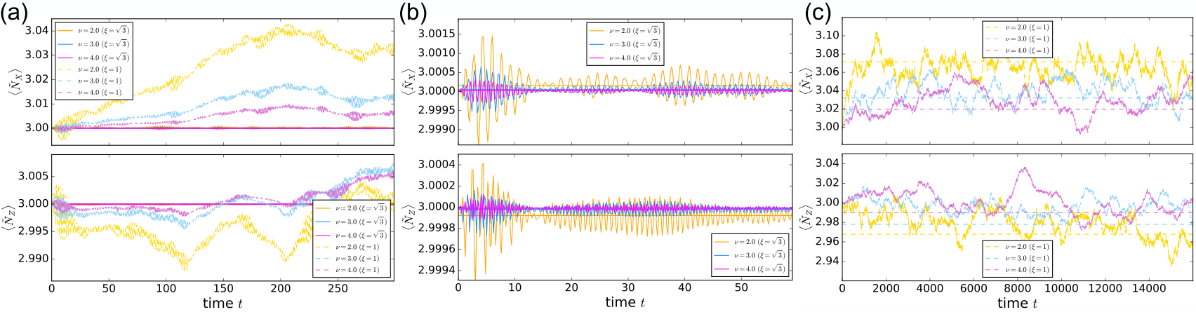
Numerical results probing the emergent U(1)$\times$U(1) symmetry and the effect of resonances are shown in Fig. 4. Using ED, we calculate the dynamics from representative initial product states of $\braket{\tilde{N}_{X}}$ and $\braket{\tilde{N}_{Z}}$ for several values of $\nu$ for both $\xi=1$ and $\xi=\sqrt{3}$. For $\xi=1$, $\braket{\tilde{N}_{X}}$ and $\braket{\tilde{N}_{Z}}$ immediately begin to exhibit strong discrepancies in comparison with their initial values, indicative of the resonant processes discussed above. For $\xi=\sqrt{3}$, however, $\braket{\tilde{N}_{X}}$ and $\braket{\tilde{N}_{Z}}$ do not strongly diverge indefinitely from their initial values. Contrarily, they begin to oscillate around saturation values close to their initial values. These saturation values are well-described by the “diagonal ensemble” Kollar and Eckstein 2008; Rigol et al. 2008; D’Alessio et al. 2016, defined for an arbitrary operator $\mathcal{O}$ in the eigenbasis $\ket{E}$ of $H$ as

$\displaystyle\braket{O}_{\rm DE}=\sum_{E}|\braket{\psi_{0}|E}|^{2}\braket{E|O|E},$

(33)

where $\ket{\psi_{0}}$ is the initial state. Physically, $\braket{O}_{\rm DE}$ is the infinite-time average of $\braket{O(t)}$; the fact that $\braket{\tilde{N}_{X,Z}}_{\rm DE}$ are so close to the values of $\braket{\tilde{N}_{X,Z}}$ at time $t=0$, and in fact become closer as $\nu$ increases, is indicative of the emergent U(1)$\times$U(1) conservation law in the limit ${\nu/g\to\infty}$. In particular, the fact that $\braket{\tilde{N}_{X,Z}}$ stabilize around these values after an initial transient suggests that the dynamics of the system can be well approximated by one that conserves both $\tilde{N}_{X}$ and $\tilde{N}_{Z}$.

To probe the lifetime of the encoded qubit in the presence of perturbations, we simulate the quench dynamics of $\braket{\tilde{\mathcal{X}}(t)}$ and $\braket{\tilde{\mathcal{Z}}(t)}$ starting from initial product states that are eigenstates of one of the logical operators. We calculate the lifetime $\tau_{X}$ ($\tau_{Z}$) as the first time at which $\braket{\tilde{\mathcal{X}}(t)}=\braket{\tilde{\mathcal{X}}}_{\rm DE}$ [$\braket{\tilde{\mathcal{Z}}(t)}=\braket{\tilde{\mathcal{Z}}}_{\rm DE}$]. We then repeat the simulation for a sequence of $g$ and $\nu$ values to extract the dependence of $\tau_{X,Z}$ on these parameters. The data, shown in Fig. 5, show a clear power-law scaling in $\nu/g$, rather than the expected stretched-exponential scaling of Eq. (26).

This deviation from the expected scaling can be understood straightforwardly as a finite-size effect. In the presence of (approximate) $\tilde{N}_{X,Z}$ conservation, only one type of process can “flip” the state of the logical qubit: an excitation is created at one of the boundaries, propagates through the bulk of the system, and is annihilated at the other boundary of the same (rough/smooth) type. If the excitation propagates between rough (smooth) boundaries, $\braket{\tilde{\mathcal{X}}}$ ($\braket{\tilde{\mathcal{Z}}}$) changes sign. This process is second-order in $g$, the energy scale for quasiparticle creation at the boundaries, and subextensive in the kinetic energy scale $J$, which propagates the excitation between boundaries. The relaxation time associated with this process for a system of size $(L_{x},L_{y})$ is then

$\displaystyle\tau_{X}\sim\frac{\nu}{g^{2}}\left(\frac{\nu}{J}\right)^{L_{y}-2},\indent\tau_{Z}\sim\frac{\nu}{g^{2}}\left(\frac{\nu}{J}\right)^{L_{x}-1}.$

(34)

In this formula, we omit constant factors and have included appropriate powers of $J$ for dimensional purposes. For sufficiently large $\nu$, these lifetimes diverge exponentially in the thermodynamic limit $L_{x},L_{y}\to\infty$. This recovers the familiar fact Kitaev 2003; Bravyi and Kitaev 1998; Fowler et al. 2012; Fendley 2016; Else et al. 2017; Kemp et al. 2017 that the encoded qubit is only stable up to exponentially small finite-size corrections (or, equivalently, exponentially long times at finite size). At the small system size $(L_{x},L_{y})=(2,3)$ considered here (due to runtime constraints, as each relaxation-time calculation involves evolving the system over times of up to $\sim 10^{4}J^{-1}$), these timescales both scale as $\nu^{2}/g^{2}$, consistent with the timescales observed in our numerics. Nevertheless, since the results of Fig. 4 suggest that the approximate U(1)$\times$U(1) symmetry is operative, we expect that the regime in which $\tau\gtrsim t_{*}$ [Eq. (26)] holds should be accessible at larger system sizes, even if numerical simulation of the system at such sizes becomes infeasible.

In summary, while our numerical results are hindered by finite-size effects, they clearly reveal the presence of a long-lived emergent U(1)$\times$U(1) symmetry despite the presence of symmetry-violating perturbations. These results are consistent with the existence of an encoded qubit with a lifetime parametrically long in the inverse of the perturbation energy scale, but larger-scale numerics would be required to validate the prediction of a stretched-exponential lifetime in this model.

A general, potentially open-system, quantum dynamical evolution on a Hilbert space $\mathcal{H}$ is described by a completely positive trace preserving (CPTP) map Nielsen and Chuang 2010 $\mathcal{E}_{t}$ on the space of operators $\mathcal{B}(\mathcal{H})$ that is a function of a discrete or continuous time parameter $t$. Here, we are interested in dynamical evolutions that retain a quantum memory of initial conditions. A very general formulation of the quantum memory condition is obtained by requiring the dynamical evolution to be correctable with respect to a chosen quantum code. More precisely, quantum memory of a subsystem $\mathcal{H}_{L}$ within the full Hilbert space $\mathcal{H}=(\mathcal{H}_{L}\otimes\mathcal{H}_{J})\oplus\mathcal{H}_{\perp}$—where $L,J,$ stand for logical and junk subsystems, respectively, and where $\perp$ denotes the orthogonal complement subspace—is retained if the dynamics under $\mathcal{E}_{t}$ is correctable. That is, there exists a recovery map $\mathcal{R}_{t}$ such that Kribs et al. 2005; Kribs et al. 2006

$\displaystyle\text{Tr}_{J}\circ P\circ\mathcal{R}_{t}\circ\mathcal{E}_{t}\,(\rho)=\text{Tr}_{J}(\rho)\,,$

(35)

for $\rho$ a density matrix supported on $\mathcal{H}_{L}\otimes\mathcal{H}_{J}$ and $P$ a projector onto $\mathcal{H}_{L}\otimes\mathcal{H}_{J}$. This definition says that $\mathcal{H}_{L}$ forms a noiseless subsystem Kribs et al. 2005; Kribs et al. 2006 for $\mathcal{R}_{t}\circ\mathcal{E}_{t}$. In particular, when $\mathcal{R}_{t}=\mathbbm{1}$ this reduces to $\mathcal{H}_{L}$ forming a noiseless subsystem for the dynamics $\mathcal{E}_{t}$. For the interesting subclass of closed-system unitary dynamics, the former condition is too weak to be nontrivial, since all unitary evolutions can in principle be undone. In this setting, we therefore focus on the latter definition, where the recovery map is taken to be $\mathcal{R}_{t}=\mathbbm{1}$ and $\mathcal{H}_{L}$ is a noiseless subsystem for $\mathcal{E}_{t}$, i.e. some initial quantum information remains static under the evolution.

While the above definition applies to perfect quantum memory for arbitrarily long times, it is interesting to loosen this to an approximate quantum memory with high probability for a sufficiently long time, as we consider in a certain setting below. It is also easy to come up with trivial examples of dynamics that retain a quantum memory, such as a single qubit with trivial evolution. We are interested in nontrivial examples where every qubit participates in the dynamics to form a quantum memory via a collective quantum many-body effect. We further want this memory to be stabilizable against generic uniform local perturbations that remain sufficiently weak.

To construct specific examples of nontrivial noiseless subsystems, we focus our attention on stabilizer subsystem codes Poulin 2005; Bacon 2006 (see also Ref. Knill et al. 2000). For the remainder of this section we restrict our attention to qubits and $\mathbb{Z}_{2}$ local degrees of freedom (i.e., qubits) for simplicity of presentation; the extension to $\mathbb{Z}_{p}$ for $p$ prime (i.e., qudits with prime dimension) is straightforward. Further extension to general $\mathbb{Z}_{N}$ is possible, however the theory of stabilizer subsystem codes for composite dimensions becomes more complicated.

stabilizer subsystem codes are defined by a group of “gauge” operators $G\leq P$ that form a subgroup of the Pauli group $P$. We remark that these “gauge” operators are not related to the gauge transformations of lattice gauge theory, but rather refer to operators acting on redundant “gauge” qubit degrees of freedom associated to $\mathcal{H}_{J}$. An auxiliary group of stabilizer operators $S$ is given by the center of the gauge group, $S=Z(G)<P$. This induces a decomposition of the Hilbert space

$\displaystyle\mathcal{H}=\bigoplus_{\{\lambda_{i}\}}(\mathcal{H}_{L}\otimes\mathcal{H}_{J})_{\{\lambda_{i}\}}$

(36)

into isomorphic sectors labelled by a complete set of stabilizer eigenvalues, specified here by the eigenvalues $(-1)^{\lambda_{i}}$ of a generating set of stabilizers $s_{i}$. Here $L$ denotes the “logical subsystem” and $J$ denotes the “junk subsystem” for reasons we now explain. The “gauge” operators act within each sector as $\mathbbm{1}_{L}\otimes g_{J}$. Operators in the commutant (i.e., centralizer) of the gauge subgroup $C(G)$ are called bare logical operators; their actions are only defined up to multiplication with elements of the stabilizer group. Therefore $L=C(G)/S$ describes the group of bare logical operators up to equivalence. These bare logical operators act within each sector as $\ell_{L}\otimes\mathbbm{1}_{J}$. As logical quantum information is only stored in the logical subsystem $\mathcal{H}_{L}$, a larger class of “dressed logical” operators are relevant. These dressed logical operators implement the same set of transformations on $\mathcal{H}_{L}$ while also potentially disturbing $\mathcal{H}_{J}$ by an unimportant operator. The algebra of dressed logical operators is given by the commutant of the stabilizer subgroup, $C(S)$. Operators in $C(S)$ have a well defined logical action up to multiplication with “gauge” operators. Hence $C(S)/G$ is the group of dressed logical operators up to equivalence. Representative dressed logical operators act within each sector as $\ell_{l}\otimes g_{J}$. The code distance $d$ is given by the minimum Pauli weight over all representative dressed logical operators. The group $L=C(G)/S$ of bare logical operators is a projective representation of the group $\mathbb{Z}_{2}^{\times|L|}$, where $|L|$ is twice the number of encoded qubits. Similarly the group $C(S)/G$ of dressed logical operators, modulo complex phases, forms a representation of the same group $\mathbb{Z}_{2}^{\times|L|}$.

The essential features of a stabilizer subsystem code are often packaged into the notation $[[n,k,r,d]]$ where $n$ denotes the number of physical qubits, $k$ the number of encoded logical qubits, $r$ the number of gauge qubits, and $d$ the code distance. In this notation, $[[n,k,0,d]]$ codes are conventional stabilizer codes. Quantum error correction for stabilizer subsystem codes is implemented by measuring the gauge generators (in a sequence that accounts for the fact they may not commute) and using this information to reconstruct the stabilizer eigenvalues. The measured stabilizer eigenvalues are then used to compute a correction operator that is applied to return the system to the code space such that the inferred error operator composed with the correction operator results in a trivial logical operation.

For concreteness we always fix a choice of generators for the gauge group, i.e., we write $G=\langle\{g_{i}\}\rangle$, where the list of generators $g_{i}$ may be overcomplete. If the generators can be picked to consist of purely $X$-type and $Z$-type Pauli operators, the code is known as a CSS subsystem code Calderbank and Shor 1996; Steane 1996. Our focus is on systems with generators $g_{i}$ that respect the microscopic locality of an underlying lattice. Furthermore, we fix a choice of generators for the stabilizer group, $S=\langle\{s_{i}\}\rangle$, which can involve a combination of local and nonlocal operators. A topological subsystem code Bombin et al. 2009; Kargarian et al. 2010; Bombin 2010; Suchara et al. 2011; Bravyi et al. 2013 is one for which the stabilizer generators can all be picked to be local with respect to an underlying lattice while the code distance $d$ is macroscopic (i.e., $d$ grows as the number of physical qubits increases).

In this subsection we discuss an interpretation of the stabilizer group of a subsystem code as an anomalous symmetry. We go on to describe the consequences that such a symmetry has on closed an open system dynamics whose generators are symmetric, of which the example in Sec. II is a special case.

The stabilizer group of a nontrivial subsystem code forms a type of anomalous symmetry. For our purposes here, an anomalous symmetry is defined by the property that no local symmetric gapped Hamiltonian can have a unique ground state. More precisely, for nontrivial $\mathcal{H}_{L}$ of dimension $2^{|L|/2}$, any Hamiltonian that is given by a sum of gauge operators, i.e.,

$\displaystyle H=\sum_{v}h_{v}\,,$

(37)

where the interactions $h_{v}$ are (linear combinations of) gauge operators, has at least a $2^{|L|/2}$-fold degeneracy of its energy levels as it commutes with the stabilizer and bare logical operators of the code. For the class of subsystem codes we consider, namely those with local generators that protect against local errors, any local Hamiltonian that commutes with the stabilizer symmetry must also commute with the bare logical operator algebra and hence must have degenerate energy levels. That is, any local Hamiltonian that respects the stabilizer symmetry group $S$, which is a linear representation of $\mathbb{Z}_{2}^{\times|S|}$, automatically respects a larger symmetry group $C(G)$ that additionally includes the bare logical algebra, which is a projective representation of $\mathbb{Z}_{2}^{\times|L|}$. Pairs of bare logical operators that define logical qubits anticommute, as an aside for readers familiar with the concept the resulting anticommutation relations can be taken to define a type of mixed anomaly valued in $H^{2}(\mathbb{Z}_{2}^{\times|L|},U(1))$ associated to the projective representation of the bare logical algebra Tachikawa 2020.

For topological subsystem codes in 2D Bombin 2010, the stabilizer symmetry is in fact a 1-form symmetry ¹¹ 1 A $k$-form symmetry is generated by operators acting on submanifolds of codimension $k$. associated to string operators of nontrivial pointlike superselection sectors Gaiotto et al. 2015. In this case the anomaly corresponds to the topological braiding phases of these pointlike sectors. In dimensions greater than two, the stabilizer symmetry of a topological subsystem code may be a higher $k$-form symmetry Bombín 2015; Kubica and Beverland 2015; Kubica and Vasmer 2021, or a more unconventional symmetry related to fracton topological order Devakul and Williamson 2021.

The time evolution $e^{-iHt}$ generated by a local Hamiltonian that commutes with a nontrivial stabilizer subsystem code symmetry, and hence takes the form introduced in Eq. (37), necessarily preserves a quantum memory as it commutes with the bare logical operators and therefore acts trivially within the $\mathcal{H}_{L}$ subsystems. More generally, any dynamical evolution generated by local terms that commute with the type of stabilizer subsystem symmetry we consider, and are hence linear combinations of gauge operators, preserve a quantum memory on $\mathcal{H}_{L}$. This includes open-system dynamics, which can be induced by unitary dynamics on an extended Hilbert space that commutes with the stabilizer symmetry on the original degrees of freedom.

For a more precise formulation of this point, consider a family of quantum channels describing time evolution parameterized by $t$,

$\displaystyle\mathcal{E}_{t}(\rho)=\sum_{i}K_{i}(t)\,\rho\,K_{i}^{\dagger}(t)\,,$

(38)

where the Kraus operators $K_{i}(t)$ are (linear combinations of) gauge operators that satisfy the trace preserving condition $\sum_{i}K_{i}^{\dagger}(t)K_{i}(t)=\mathbbm{1}$. For the simple case of closed-system unitary evolution discussed above we have only a single Kraus operator $K(t)=e^{-iHt}$ for $H$ a local Hamiltonian of the form described in Eq. (37). This description also applies more generally, including in the case of monitored dynamics involving quantum measurements, in which case some Kraus operators may take the form of projections onto the eigenvalues of gauge operators, e.g., $K_{i}(t)=\frac{1}{2}(\mathbbm{1}-g_{i})$ for a gauge operator $g_{i}$. In fact, the quantum memory we are discussing exists even at the level of individual quantum trajectories, where projective measurements are made without averaging over the measurement outcomes.

Any dynamics generated by local terms that respect a nontrivial stabilizer subsystem code symmetry (that corrects local errors) must take the form introduced in Eq. (38). Hence the symmetry condition implies that the dynamics preserves a quantum memory, i.e., commutes with the bare logical algebra. The preservation of the quantum memory can be understood as a consequence of the mixed anomaly associated to the stabilizer subsystem code symmetry, see above.

We emphasize that, in fixed stabilizer eigenspaces, the dynamics within the junk subsystem $\mathcal{H}_{J}$ can be totally generic or chaotic, or alternatively may be integrable such as when only a commuting set of gauge operators enters the dynamics, or in the simple case of conventional stabilizer codes where $\mathcal{H}_{J}$ is trivial.

In the presence of Hamiltonian perturbations and couplings to the environment that do not respect the stabilizer symmetry, the dynamics generated by a stabilizer subsystem code may no longer protect $\mathcal{H}_{\rm L}$ in Eq. (36) as a noiseless subsystem. To maintain protection of the quantum information in these subsystems, the most systematic approach is the implementation of quantum error correction, either through active measures or by passively relying on a sufficiently low temperature environment Dennis et al. 2001; Bacon 2006. This is an interesting direction with many facets that we leave to future work. Here we restrict our focus to passive extension of quantum memory lifetimes under closed-system unitary dynamics in the presence of nonsymmetric Hamiltonian perturbations, which may correspond to control errors. We rely on recently established results on prethermal quantum memories proved in Ref. Else et al. 2017; Else et al. 2020.

The results of Ref. Else et al. 2017; Else et al. 2020 apply to dynamics generated by Hamiltonians of the form

$\displaystyle H=H_{0}+gV+\nu_{1}\Sigma_{1}+\dots+\nu_{K}\Sigma_{K}\,,$

(39)

where $H_{0}$ is a local Hamiltonian that obeys a U(1)^×K symmetry generated by the operators $\Sigma_{k}$ ($k=1,\dots,K$), and $V$ is a sum of symmetry-breaking local perturbations [with O(1) operator norm] with $g$ sufficiently small compared to all the $\nu_{i}$. Note that both $H_{0}$ and $V$ generically contain non-commuting local terms, and that $H_{0}$ can be nonintegrable. In order for the prethermalization arguments to hold, the U(1) generators $\Sigma_{k}$ must be sums of commuting local terms—in Sec. III.5.1 we consider an example of a stabilizer subsystem code to which these prethermalization arguments cannot be applied due to nonlocality of the $\Sigma_{k}$. We demonstrate below that a sufficient condition guaranteeing that the $\Sigma_{k}$ are sums of commuting local terms is for the underlying subsystem code to be a topological subsystem code. In the context of quantum memory, the crucial U(1)^×K symmetry is in fact closely related to a pair of stabilizer (subsystem) codes that we refer to as the local and global codes, which we now explain. We refer back to the example in Sec. II throughout the more general explanation.

First, we specify the local subsystem code via a choice of stabilizer generators $S=\langle\{s_{i}\}\rangle$. As the name suggests, our focus is on cases where these generators have local support on a spatial lattice for practical reasons ²² 2 However, we consider at least one example where this is not the case.. These stabilizer generators are given by star and plaquette terms for the example in Sec. II. There may be relations (i.e., redundancies) among these generators; we label a generating set of such relations as $\{r_{j}\}$, where the relations $r_{j}$ are defined such that

$\displaystyle\prod_{i\in r_{j}}s_{i}=\mathbbm{1}\,.$

(40)

In the example introduced in Sec. II there are no such relations. Next, we define the group of gauge operators $G$ to be generated by all local operators contained in $C(S)$. Finally, the set of bare logical operators for the local code is given by $L=C(G)/S$. We demand that all elements of $L$ have macroscopic weight (if any were local those would already be included in $G$). We assume that the dimension $2^{|L|/2}$ of the logical algebra is at least two, otherwise there would be no quantum memory even for unperturbed dynamics. The logical operators are macroscopic string operators in the example covered in Sec. II. The local stabilizer subsystem code defines a block decomposition of the Hilbert space according to the eigenvalues of the stabilizer generators $\frac{1}{2}(\mathbbm{1}-s_{i})={\lambda_{i}}$, see Eq. (36). Here, there may be nontrivial relations $r_{j}$ due to the the choice of generators being overcomplete. In this case, the blocks in Eq. (36) labelled by eigenvalues not satisfying the relation conditions in Eq. (40) are empty. In the example introduced in Sec. II these sectors correspond to configurations of pinned $e$ and $m$ anyons in the surface code.

We now move on to define the U(1)^×K symmetry, and the global stabilizer subsystem code, in terms of the stabilizers of the local subsystem code. As above, each stabilizer generator defines an occupation number $\lambda_{i}\in\{0,1\}$ via the eigenvalue of $\frac{1}{2}(\mathbbm{1}-s_{i})$. Any subset of stabilizer generators $S_{k}\subseteq\{s_{i}\}$ (that involves an increasing number of generators as the number of physical qubits grows) defines a generator of a U(1) symmetry via

$\displaystyle\Sigma_{k}:=\sum_{s_{i}\in S_{k}}\frac{1}{2}(\mathbbm{1}-s_{i})\,.$

(41)

A sufficient condition that guarantees the locality of the $\Sigma_{k}$ defined above is for the underlying local stabilizer subsystem code to be a topological subsystem code. In such codes, the stabilizers $s_{i}$ are local and mutually commuting by definition (see Sec. III.2). Conversely, a U(1) symmetry generated by a sum of mutually commuting local Pauli terms always defines a topological stabilizer subgroup generated by those terms. The local code in Sec. II is simply the topological surface code, and the U(1)$\times$U(1) symmetry corresponds to $e$ and $m$ anyon number conservation.

The U(1) symmetry generated by $\Sigma_{k}$ enforces conservation of the total occupation number, $\sum\lambda_{i}^{(k)}$, of the stabilizers included in the set $S_{k}$. This induces a block decomposition of the Hilbert space,

$\displaystyle\bigoplus_{\{n_{k}\}}\Big(\mathcal{H}_{L}\otimes\bigoplus_{\{\lambda_{i}\}:\sum\lambda_{i}^{(k)}=n_{k}}{\mathcal{H}_{J}}_{\{\lambda_{i}\}}\Big)_{\{n_{k}\}}\,,$

(42)

which is strictly coarser than the decomposition induced by the local stabilizer code symmetry, introduced in Eq. (36). In particular, all blocks of the local stabilizer symmetry that satisfy $\sum\lambda_{i}^{(k)}=n_{k}$, for the stabilizer generators in the set $S_{k}$, are collected into the single $\{n_{k}\}$ block of the U(1)^×K symmetry. In the surface code example from Sec. II the blocks correspond to states with fixed $e$ and $m$ anyon number, collecting many different configurations with the same numbers of $e$ and $m$ anyons. The gauge operators of the local stabilizer code remain symmetric under the U(1)^×K symmetry. In addition, arbitrary local operators can be projected onto fixed occupation number eigenspaces of the overlapping local stabilizers $\frac{1}{2}(\mathbbm{1}-s_{i})$ to produce further symmetric local operators. For example, the gauge generators of the global stabilizer code introduced below can be projected in this way to create symmetric local operators, as was done for the example in section II.6.

Finally, we move on to define the global stabilizer subsystem code. Each set of stabilizers $S_{k}$ introduced above, that is not a stabilizer relation, defines a nontrivial $\mathbb{Z}_{2}$ subgroup of both the U(1) symmetry and the local stabilizer symmetry. This subgroup is generated by a $\pi$ rotation of the form

$\displaystyle e^{i\pi\Sigma_{k}}=\prod_{i\in S_{k}}s_{i}\,,$

(43)

which enforces conservation mod 2 of the occupation number of stabilizers in $S_{k}$. If $S_{k}$ is a relation, the above rotation by $\pi$ is trivial i.e. $e^{i\pi\Sigma_{k}}=\mathbbm{1}$ and the conservation of the occupation of stabilizers in $S_{k}$ mod 2 is a constraint (also known as a materialized symmetry Kitaev 2003; Brown and Williamson 2020). For example, consider the toric code with periodic boundary conditions Kitaev 2003; in this case, the global stabilizers $S_{X}$ and $S_{Z}$, consisting of the product of all star and plaquette stabilizers, respectively, are both relations (i.e., $S_{X}=S_{Z}=\mathbbm{1}$). The global stabilizer code is thus trivial (i.e., has trivial generators) and hence does not protect a quantum memory, even under dynamics that respect the U(1)$\times$U(1) symmetry corresponding to conservation of the total number of “electric” and “magnetic” anyons. To see this, note that an anyon can move around a noncontractible cycle of the torus, inducing a nontrivial logical action, via local steps that preserve the U(1)$\times$U(1) symmetry Else et al. 2017. This is no longer possible with the surface-code-like open boundary conditions considered in Section II. There the products over all star and plaquette operators, respectively, correspond to nontrivial boundary operators.

In the nontrivial case where $S_{k}$ is not a relation, the global stabilizer group is generated by the operators $\{e^{i\pi\Sigma_{k}}\}$ which induce a block decomposition

$\displaystyle\bigoplus_{\{\sigma_{j}\}}\bigg(\mathcal{H}_{L}\otimes\bigoplus_{\{\lambda_{i}\}:\sum\lambda_{i}^{(j)}=\sigma_{j}}{\mathcal{H}_{J}}_{\{\lambda_{i}\}}\bigg)_{\{\sigma_{j}\}}\,,$

(44)

where $\sum\lambda_{i}^{(j)}=\sigma_{j}$ is only required to hold mod 2, with the sum taken over the set $S_{j}$ and with $\sigma_{j}=\frac{1}{2}(\mathbbm{1}-e^{i\pi\Sigma_{j}})$ the eigenvalue of the global stabilizer. In the example from Sec. II the block decomposition corresponds to the conservation of both $e$ and $m$ parity. Once again we define the the gauge group to be generated by all local operators that commute with all global stabilizers. This group contains all the gauge generators of the local stabilizer code. The bare logical operators are then given by the commutant of the gauge group, up to multiplication with stabilizers. Each bare logical must also be a bare logical of the local stabilizer code. The dressed logical operators for the global stabilizer code may be significantly lower weight than those of the local stabilizer code, due to the enlarged gauge group. In particular, the dressed logical operators may have constant weight, although by definition they must remain nonlocal otherwise they would have been included in the gauge group. The global stabilizer code may only be an error detecting code, even when the local stabilizer code is an error correcting code. However this is sufficient to preserve a quantum memory in a noiseless subsystem. For the example in Sec. II the gauge generators include single site Pauli operators in the bulk, and two body Pauli operators along the boundary. The dressed logical operators become two body on a pair of well separated boundaries and the global code is simply an error detecting code for certain single qubit errors on the boundary. For the examples of subsystem codes considered in Sec. III.5, the global stabilizers act exclusively on the boundaries and indeed define single-Pauli error detecting codes there. In general, the global code should be a nontrivial error detecting code with no spatially local (dressed) logical operators. This suffices to ensure the persistence of a prethermal quantum memory under the dynamical evolution with U(1)^×K symmetry breaking perturbations introduced in Eq. (39).

As discussed in section III.3, dynamics generated by a Hamiltonian that is a sum of gauge generators for the global subsystem code preserves a quantum memory associated to the noiseless subsystem $\mathcal{H}_{L}$. However, in the presence of generic local Hamiltonian perturbations we cannot provide a guarantee that this memory persists. For the stricter setting of dynamics generated by a local Hamiltonian obeying the full U(1)^×K symmetry we can apply the results of Refs. Else et al. 2017; Else et al. 2020 to ensure the existence of a prethermal memory time $t_{*}$ that is a stretched exponential in a parameter that measures the relative perturbation strength in a Hamiltonian of the form (39). The results of Refs. Else et al. 2017; Else et al. 2020 imply that such a Hamiltonian $H$ can be expanded in a U(1)^×K-symmetric perturbation series that is convergent up to an order proportional to $(\nu/g)^{1/K}$, where $\nu\equiv\sqrt{\sum^{K}_{i=1}\nu^{2}_{i}}$. This in turn implies that the evolution $e^{-itH}$ generated by the above Hamiltonian retains the U(1)^×K symmetry, up to small corrections, until a time

$\displaystyle t_{*}\gtrsim e^{C(\nu/g)^{1/K}},$

(45)

where $C>0$ is a constant. In particular this implies that the perturbed evolution commutes with the global stabilizer symmetry up to small corrections, which in turn implies the preservation of a quantum memory associated to a noiseless subsystem. We may also choose to strictly enforce some subset of stabilizer symmetries, while enforcing others via a $U(1)^{\times K^{\prime}}$ symmetry that is then allowed to be broken by sufficiently weak perturbations and similar results follow Else et al. 2017; Else et al. 2020.

The formalism outlined in Secs. III.1–III.4 yields a simple recipe for defining nontrivial quantum dynamics that preserves quantum information encoded in the initial state. In the most general case, any local quantum circuit composed of unitary gates generated by local products of the gauge generators $g_{i}\in G$ will preserve information encoded in the logical subsystem $\mathcal{H}_{L}$. Furthermore, one can allow hybrid unitary-projective circuits in which unitary dynamics is interspersed with projective local measurements, provided that the measurement operators are also local products of gauge generators. Alternatively, one can consider dynamics generated by a local Hamiltonian consisting of a sum over local products of gauge generators. Such models (and perturbations thereof) are studied in Secs. II.5 and II.6.

Regardless of their nature (i.e., whether they are Hamiltonian, unitary, or unitary-projective), the dynamics constructed in this way possess a symmetry group equal to the stabilizer group $S$. When the generators of the stabilizer group act on all lattice sites at once, the dynamics preserve a global symmetry, e.g. the $\mathbb{Z}_{2}\times\mathbb{Z}_{2}$ global symmetry of Sec. II, that protects the encoded quantum memory. Depending on the structure of the stabilizer group, the protecting symmetry can be a global, subsystem, or higher-form symmetry Gaiotto et al. 2015; Vijay et al. 2016; Williamson 2016.

In this section, we consider several examples of such families of quantum dynamics and elucidate their essential features. We present in Appendix B a high-level discussion of other examples based on a variety of stabilizer codes in three or fewer spatial dimensions.

References

- Hayden and Preskill (2007) P. Hayden and J. Preskill, Journal of High Energy Physics 0709, 120–120 (2007).
- Sekino and Susskind (2008) Y. Sekino and L. Susskind, Journal of High Energy Physics 0810, 065–065 (2008).
- Lashkari et al. (2013) N. Lashkari, D. Stanford, M. Hastings, T. Osborne, and P. Hayden, Journal of High Energy Physics 1304 (2013).
- Landsman et al. (2019) K. A. Landsman, C. Figgatt, T. Schuster, N. M. Linke, B. Yoshida, N. Y. Yao, and C. Monroe, Nature 567, 61 (2019).
- Deutsch (1991) J. M. Deutsch, Phys. Rev. A 43, 2046 (1991).
- Srednicki (1994) M. Srednicki, Phys. Rev. E 50, 888 (1994).
- Rigol et al. (2008) M. Rigol, V. Dunjko, and M. Olshanii, Nature 452, 854 (2008).
- D’Alessio et al. (2016) L. D’Alessio, Y. Kafri, A. Polkovnikov, and M. Rigol, Adv. Phys. 65, 239 (2016).
- Deutsch (2018) J. M. Deutsch, Rep. Prog. Phys. 81, 082001 (2018).
- Shor (1995) P. W. Shor, Phys. Rev. A 52, R2493 (1995).
- Aharonov and Ben-Or (2008) D. Aharonov and M. Ben-Or, SIAM Journal on Computing 38, 1207 (2008), arXiv:9906129 [quant-ph] .
- Knill et al. (1998) E. Knill, R. Laflamme, and W. H. Zurek, Proceedings of the Royal Society A: Mathematical, Physical and Engineering Sciences 454, 365 (1998), arXiv:9702058 [quant-ph] .
- Kitaev (2003) A. Y. Kitaev, Annals of Physics 303, 2 (2003).
- Bravyi and Kitaev (1998) S. B. Bravyi and A. Y. Kitaev, arXiv:quant-ph/9811052 (1998).
- Dennis et al. (2001) E. Dennis, A. Kitaev, A. Landahl, and J. Preskill, Journal of Mathematical Physics 43, 4452 (2001).
- Bacon (2006) D. Bacon, Phys. Rev. A 73, 012340 (2006).
- Brown et al. (2016a) B. J. Brown, D. Loss, J. K. Pachos, C. N. Self, and J. R. Wootton, Rev. Mod. Phys. 88, 45005 (2016a).
- Nandkishore and Huse (2015) R. Nandkishore and D. A. Huse, Annu. Rev. Condens. Matter Phys 6, 15 (2015).
- Altman and Vosk (2015) E. Altman and R. Vosk, Annu. Rev. Condens. Matter Phys 6, 383 (2015).
- Abanin et al. (2019) D. A. Abanin, E. Altman, I. Bloch, and M. Serbyn, Rev. Mod. Phys. 91, 021001 (2019).
- Žnidarič et al. (2008) M. Žnidarič, T. Prosen, and P. Prelovšek, Phys. Rev. B 77, 064426 (2008).
- Bardarson et al. (2012) J. H. Bardarson, F. Pollmann, and J. E. Moore, Phys. Rev. Lett. 109, 017202 (2012).
- Serbyn et al. (2013a) M. Serbyn, Z. Papić, and D. A. Abanin, Phys. Rev. Lett. 111, 127201 (2013a).
- Serbyn et al. (2013b) M. Serbyn, Z. Papić, and D. A. Abanin, Phys. Rev. Lett. 110, 260601 (2013b).
- Huse et al. (2014) D. A. Huse, R. Nandkishore, and V. Oganesyan, Phys. Rev. B 90, 174202 (2014).
- Swingle (2013) B. Swingle, arXiv preprint arXiv:1307.0507 (2013).
- Imbrie et al. (2017) J. Z. Imbrie, V. Ros, and A. Scardicchio, Annalen der Physik 529, 1600278 (2017).
- Huse et al. (2013) D. A. Huse, R. Nandkishore, V. Oganesyan, A. Pal, and S. L. Sondhi, Phys. Rev. B 88, 014206 (2013).
- Chandran et al. (2014) A. Chandran, V. Khemani, C. R. Laumann, and S. L. Sondhi, Phys. Rev. B 89, 144201 (2014).
- Bahri et al. (2015) Y. Bahri, R. Vosk, E. Altman, and A. Vishwanath, Nature Communications 6, 1 (2015).
- Nandkishore et al. (2014) R. Nandkishore, S. Gopalakrishnan, and D. A. Huse, Phys. Rev. B 90, 064203 (2014).
- Nandkishore and Gopalakrishnan (2016) R. Nandkishore and S. Gopalakrishnan, Annalen der Physik 529, 1600181 (2016).
- Levi et al. (2016) E. Levi, M. Heyl, I. Lesanovsky, and J. P. Garrahan, Phys. Rev. Lett. 116, 237203 (2016).
- Fischer et al. (2016) M. H. Fischer, M. Maksymenko, and E. Altman, Phys. Rev. Lett. 116, 160401 (2016).
- De Roeck and Huveneers (2017) W. De Roeck and F. Huveneers, Phys. Rev. B 95, 155129 (2017).
- Luitz et al. (2017) D. J. Luitz, F. Huveneers, and W. De Roeck, Phys. Rev. Lett. 119, 150602 (2017).
- Rubio-Abadal et al. (2019) A. Rubio-Abadal, J.-y. Choi, J. Zeiher, S. Hollerith, J. Rui, I. Bloch, and C. Gross, Phys. Rev. X 9, 041014 (2019).
- Bauer and Nayak (2013) B. Bauer and C. Nayak, Journal of Statistical Mechanics: Theory and Experiment 2013, P09005 (2013).
- Wahl and Béri (2020) T. B. Wahl and B. Béri, Phys. Rev. Research 2, 033099 (2020).
- De Roeck and Imbrie (2017) W. De Roeck and J. Z. Imbrie, Philos. Trans. R. Soc. A 375, 20160422 (2017).
- Wahl et al. (2018) T. B. Wahl, A. Pal, and S. H. Simon, Nature Physics 15, 164–169 (2018).
- Gopalakrishnan and Huse (2019) S. Gopalakrishnan and D. A. Huse, Phys. Rev. B 99, 134305 (2019).
- Doggen et al. (2020) E. V. H. Doggen, I. V. Gornyi, A. D. Mirlin, and D. G. Polyakov, Phys. Rev. Lett. 125, 155701 (2020).
- Chertkov et al. (2021) E. Chertkov, B. Villalonga, and B. K. Clark, Phys. Rev. Lett. 126, 180602 (2021).
- Decker et al. (2021) K. S. C. Decker, D. M. Kennes, and C. Karrasch, arXiv preprint arXiv:2106.12861 (2021).
- Théveniaut et al. (2020) H. Théveniaut, Z. Lan, G. Meyer, and F. Alet, Phys. Rev. Research 2, 033154 (2020).
- Pietracaprina and Alet (2021) F. Pietracaprina and F. Alet, SciPost Phys. 10, 44 (2021).
- Pai and Pretko (2019) S. Pai and M. Pretko, Phys. Rev. Lett. 123, 136401 (2019).
- Sala et al. (2020) P. Sala, T. Rakovszky, R. Verresen, M. Knap, and F. Pollmann, Phys. Rev. X 10, 011047 (2020).
- Khemani et al. (2020) V. Khemani, M. Hermele, and R. Nandkishore, Phys. Rev. B 101, 174204 (2020).
- Rakovszky et al. (2020) T. Rakovszky, P. Sala, R. Verresen, M. Knap, and F. Pollmann, Phys. Rev. B 101, 125126 (2020).
- Moudgalya et al. (2020) S. Moudgalya, B. A. Bernevig, and N. Regnault, Phys. Rev. B 102, 195150 (2020).
- Yang et al. (2020) Z.-C. Yang, F. Liu, A. V. Gorshkov, and T. Iadecola, Phys. Rev. Lett. 124, 207602 (2020).
- Moudgalya and Motrunich (2021) S. Moudgalya and O. I. Motrunich, arXiv preprint arXiv:2108.10324 (2021).
- Moudgalya et al. (2021) S. Moudgalya, B. A. Bernevig, and N. Regnault, arXiv preprint arXiv:2109.00548 (2021).
- Buča et al. (2020) B. Buča, A. Purkayastha, G. Guarnieri, M. T. Mitchison, D. Jaksch, and J. Goold, arXiv preprint arXiv:2008.11166 (2020).
- Buča (2021) B. Buča, arXiv preprint arXiv:2108.13411 (2021).
- Kitaev (2001) A. Y. Kitaev, Physics-Uspekhi 44, 131–136 (2001).
- Fendley (2012) P. Fendley, Journal of Statistical Mechanics: Theory and Experiment , P11020 (2012).
- Fendley (2016) P. Fendley, J. Phys. A: Math. Theor. 49, 30LT01 (2016).
- Kemp et al. (2017) J. Kemp, N. Y. Yao, C. R. Laumann, and P. Fendley, J. Stat. Mech. 2017, 063105 (2017).
- Else et al. (2017) D. V. Else, P. Fendley, J. Kemp, and C. Nayak, Physical Review X 7, 041062 (2017).
- Roberts et al. (2017) S. Roberts, B. Yoshida, A. Kubica, and S. D. Bartlett, Phys. Rev. A 96 (2017).
- Roberts and Bartlett (2020) S. Roberts and S. D. Bartlett, Physical Review X 10 (2020), 10.1103/PhysRevX.10.031041, arXiv:1805.01474 .
- Roberts and Williamson (2020) S. Roberts and D. J. Williamson, arXiv preprint arXiv:2011.04693 (2020).
- Stahl and Nandkishore (2021) C. Stahl and R. Nandkishore, Phys. Rev. B 103 (2021).
- Bombin et al. (2009) H. Bombin, M. Kargarian, and M. A. Martin-Delgado, Physical Review B - Condensed Matter and Materials Physics 80 (2009), 10.1103/PhysRevB.80.075111, arXiv:0811.0911 .
- Kargarian et al. (2010) M. Kargarian, H. Bombin, and M. A. Martin-Delgado, New Journal of Physics 12 (2010).
- Bombin (2010) H. Bombin, Phys. Rev. A 81, 032301 (2010).
- Suchara et al. (2011) M. Suchara, S. Bravyi, and B. Terhal, Journal of Physics A: Mathematical and Theoretical 44, 155301 (2011).
- Bravyi et al. (2013) S. Bravyi, G. Duclos-Cianci, D. Poulin, and M. Suchara, Quantum Information and Computation 13, 963 (2013).
- Li et al. (2018) Y. Li, X. Chen, and M. P. A. Fisher, Phys. Rev. B 98, 205136 (2018).
- Skinner et al. (2019) B. Skinner, J. Ruhman, and A. Nahum, Phys. Rev. X 9, 031009 (2019).
- Li et al. (2019) Y. Li, X. Chen, and M. P. A. Fisher, Phys. Rev. B 100, 134306 (2019).
- Chan et al. (2019) A. Chan, R. M. Nandkishore, M. Pretko, and G. Smith, Phys. Rev. B 99, 224307 (2019).
- Gullans and Huse (2020) M. J. Gullans and D. A. Huse, Phys. Rev. X 10, 041020 (2020).
- Choi et al. (2020) S. Choi, Y. Bao, X.-L. Qi, and E. Altman, Phys. Rev. Lett. 125, 030505 (2020).
- Fan et al. (2021) R. Fan, S. Vijay, A. Vishwanath, and Y.-Z. You, Phys. Rev. B 103, 174309 (2021).
- Fidkowski et al. (2021) L. Fidkowski, J. Haah, and M. B. Hastings, Quantum 5, 382 (2021).
- Sang and Hsieh (2021) S. Sang and T. H. Hsieh, Phys. Rev. Research 3, 023200 (2021).
- Lavasani et al. (2021) A. Lavasani, Y. Alavirad, and M. Barkeshli, Nature Physics 17, 342–347 (2021).
- Ippoliti et al. (2021) M. Ippoliti, M. J. Gullans, S. Gopalakrishnan, D. A. Huse, and V. Khemani, Physical Review X 11 (2021), 10.1103/PhysRevX.11.011030, arXiv:2004.09560 .
- Lavasani et al. (2020) A. Lavasani, Y. Alavirad, and M. Barkeshli, arXiv preprint arXiv:2011.06595 (2020).
- Abanin et al. (2017) D. Abanin, W. De Roeck, W. W. Ho, and F. Huveneers, Communications in Mathematical Physics 354, 809 (2017).
- Else et al. (2020) D. V. Else, W. W. Ho, and P. T. Dumitrescu, Phys. Rev. X 10, 021032 (2020).
- Poulin (2005) D. Poulin, Phys. Rev. Lett. 95, 230504 (2005).
- Freedman and Meyer (2001) M. H. Freedman and D. A. Meyer, Foundations of Computational Mathematics 1, 325 (2001).
- Fowler et al. (2012) A. G. Fowler, M. Mariantoni, J. M. Martinis, and A. N. Cleland, Phys. Rev. A 86, 032324 (2012).
- Fendley and Schoutens (2005) P. Fendley and K. Schoutens, Phys. Rev. Lett. 95, 046403 (2005).
- Oganesyan and Huse (2007) V. Oganesyan and D. A. Huse, Phys. Rev. B 75, 155111 (2007).
- Pal and Huse (2010) A. Pal and D. A. Huse, Phys. Rev. B 82, 174411 (2010).
- Atas et al. (2013) Y. Y. Atas, E. Bogomolny, O. Giraud, and G. Roux, Phys. Rev. Lett. 110, 084101 (2013).
- Page (1993) D. N. Page, Phys. Rev. Lett. 71, 1291 (1993).
- Brown et al. (2017) B. J. Brown, K. Laubscher, M. S. Kesselring, and J. R. Wootton, Phys. Rev. X 7, 021029 (2017).
- Satzinger et al. (2021) K. J. Satzinger, Y.-J. Liu, A. Smith, C. Knapp, M. Newman, C. Jones, Z. Chen, C. Quintana, X. Mi, A. Dunsworth, and et al., Science 374, 1237–1241 (2021).
- Kollar and Eckstein (2008) M. Kollar and M. Eckstein, Phys. Rev. A 78, 013626 (2008).
- Nielsen and Chuang (2010) M. A. Nielsen and I. L. Chuang, Quantum Computation and Quantum Information (2010).
- Kribs et al. (2005) D. Kribs, R. Laflamme, and D. Poulin, Phys. Rev. Lett. 94 (2005), 0412076 .
- Kribs et al. (2006) D. W. Kribs, R. Laflamme, D. Poulin, and M. Lesosky, Quantum Information and Computation 6, 382 (2006).
- Knill et al. (2000) E. Knill, R. Laflamme, and L. Viola, Phys. Rev. Lett. 84, 2525 (2000).
- Calderbank and Shor (1996) A. R. Calderbank and P. W. Shor, Phys. Rev. A 54, 1098 (1996).
- Steane (1996) A. M. Steane, Phys. Rev. A 54, 4741 (1996).
- Tachikawa (2020) Y. Tachikawa, SciPost Physics 8, 015 (2020).
- (104) A -form symmetry is generated by operators acting on submanifolds of codimension .
- Gaiotto et al. (2015) D. Gaiotto, A. Kapustin, N. Seiberg, and B. Willett, Journal of High Energy Physics 2015, 1 (2015), arXiv:1412.5148 .
- Bombín (2015) H. Bombín, New Journal of Physics 17 (2015).
- Kubica and Beverland (2015) A. Kubica and M. E. Beverland, Phys. Rev. A 91 (2015).
- Kubica and Vasmer (2021) A. Kubica and M. Vasmer, arXiv preprint arXiv:2106.02621 (2021).
- Devakul and Williamson (2021) T. Devakul and D. J. Williamson, Quantum 5, 438 (2021).
- (110) However, we consider at least one example where this is not the case.
- Brown and Williamson (2020) B. J. Brown and D. J. Williamson, Phys. Rev. Research 2, 1 (2020).
- Vijay et al. (2016) S. Vijay, J. Haah, and L. Fu, Phys. Rev. B (2016).
- Williamson (2016) D. J. Williamson, Phys. Rev. B 94 (2016).
- Viola et al. (1999) L. Viola, E. Knill, and S. Lloyd, Phys. Rev. Lett. 82, 2417 (1999).
- Tran et al. (2021) M. C. Tran, Y. Su, D. Carney, and J. M. Taylor, PRX Quantum 2, 010323 (2021).
- Hastings and Haah (2021) M. B. Hastings and J. Haah, arXiv preprint arXiv:2107.02194 (2021).
- Gidney et al. (2021) C. Gidney, M. Newman, A. Fowler, and M. Broughton, arXiv preprint arXiv:2108.10457 (2021).
- Bravyi and Haah (2013) S. Bravyi and J. Haah, Phys. Rev. Lett. 111, 200501 (2013).
- Bombin (2015) H. Bombin, Phys. Rev. X 5 (2015).
- Brown et al. (2016b) B. J. Brown, N. H. Nickerson, and D. E. Browne, Nature Communications 7 (2016b).
- Haah (2011) J. Haah, Phys. Rev. A 83 (2011).
- Kim and Haah (2016) I. H. Kim and J. Haah, Physical Review Letters 116, 027202 (2016).
- Prem et al. (2017) A. Prem, J. Haah, and R. Nandkishore, Physical Review B 95, 155133 (2017).
- Krinner et al. (2021) S. Krinner, N. Lacroix, A. Remm, A. D. Paolo, E. Genois, C. Leroux, C. Hellings, S. Lazar, F. Swiadek, J. Herrmann, G. J. Norris, C. K. Andersen, M. Müller, A. Blais, C. Eichler, and A. Wallraff, “Realizing repeated quantum error correction in a distance-three surface code,” (2021), arXiv:2112.03708 [quant-ph] .
- Zhao et al. (2021) Y. Zhao, Y. Ye, H.-L. Huang, Y. Zhang, D. Wu, H. Guan, Q. Zhu, Z. Wei, T. He, S. Cao, F. Chen, T.-H. Chung, H. Deng, D. Fan, M. Gong, C. Guo, S. Guo, L. Han, N. Li, S. Li, Y. Li, F. Liang, J. Lin, H. Qian, H. Rong, H. Su, L. Sun, S. Wang, Y. Wu, Y. Xu, C. Ying, J. Yu, C. Zha, K. Zhang, Y.-H. Huo, C.-Y. Lu, C.-Z. Peng, X. Zhu, and J.-W. Pan, “Realizing an error-correcting surface code with superconducting qubits,” (2021), arXiv:2112.13505 [quant-ph] .
- Bombin and Martin-Delgado (2007) H. Bombin and M. A. Martin-Delgado, Phys. Rev. B 75 (2007).
- Castelnovo and Chamon (2007) C. Castelnovo and C. Chamon, Phys. Rev. B 76 (2007).
- Castelnovo and Chamon (2008) C. Castelnovo and C. Chamon, Phys. Rev. B 78 (2008).
- Kubica et al. (2015) A. Kubica, B. Yoshida, and F. Pastawski, New Journal of Physics 17, 83026 (2015).
- Else and Nayak (2017) D. V. Else and C. Nayak, Physical Review B 96 (2017).
- Dua et al. (2019) A. Dua, I. H. Kim, M. Cheng, and D. J. Williamson, Phys. Rev. B 100 (2019).