Chapter 1Hot Neutron Star Matter and Proto Neutron Stars

Chapter 1 Hot Neutron Star Matter and Proto Neutron Stars

Fridolin Weber

William Spinella

Germán Malfatti^∗, Milva G. Orsaria^∗∗

Ignacio F. Ranea-Sandoval

Abstract: In this chapter, we investigate the structure and composition of hot neutron star matter and proto-neutron stars. Such objects are made of baryonic matter that is several times denser than atomic nuclei and tens of thousands of times hotter than the matter in the core of our Sun. The relativistic finite-temperature Green function formalism is used to formulate the expressions that determine the properties of such matter in the framework of the density-dependent mean field approach. Three different sets of nuclear parametrizations are used to solve the many-body equations and to determine the models for the equation of state of ultra-hot and dense stellar matter. The meson-baryon coupling schemes and the role of the $\Delta(1232)$ baryon in proto-neutron star matter are investigated in great detail. Using the non-local three-flavor Nambu–-Jona-Lasinio model to describe quark matter, the hadron-quark composition of dense baryonic matter at zero temperature is discussed. General relativistic models of non-rotating as well as rotating proto-neutron stars are presented in part two of our study.

Keywords: proto-neutron stars; neutron stars; nuclear equation of state; nuclear field theory; quark matter.

1 Introduction

Within a few million years after a massive star ( $\gtrsim 8\,M_{\odot}$ ) is born, its core undergoes nuclear fusion reactions that will result in a dense, heavy iron center. Up until the formation of an iron core, the massive star has been supported from collapsing by the energy released from fusing lighter elements into iron and electron degeneracy pressure (Mezzacappa 2005; Janka 2012; Foglizzo 2016; Burrows and Vartanyan 2021). When an iron core is formed, the fusion processes and subsequent energy cease; at this point, the star can no longer support its mass against the force of gravity and will begin to rapidly collapse in the span of just a few milliseconds. At this moment, the core’s temperature skyrockets and the density surpasses the point of electron degeneracy, sparking the formation of neutrons through electron capture,

\displaystyle p+e^{-}\rightarrow n^{0}+\nu_{e}\,,

(1)

where $p$ , a proton, and $e^{-}$ , an electron, combine to form a neutron, $n^{0}$ , and an electron neutrino, $\nu_{e}$ . These neutrinos are released carrying large quantities of energy, contracting the core further. The density of the core increases until it reaches nuclear density (baryon number density of around $0.16~{\rm fm}^{-3}$ , mass density of or $2.65\times 10^{14}~{\rm g/cm}^{3}$ ), where nucleon degeneracy pressure halts the collapse. Parts of the core surpassing nuclear density, like the inner most part of the core, will rebound to create a shock wave as the exterior core layers are expelled. Over the next tens of seconds, the shock wave reverses the inward trajectory of the collapsing stellar material as it moves through the stellar envelope, partially cooling the extreme temperature and contracting the material it passes through. The shock wave alone does not possess enough energy to pass through the entire stellar envelope and complete the supernova explosion; the shock wave is revived by the massive quantities of neutrinos created alongside neutrons. While most neutrinos are expelled, some remain trapped behind the shock wave, increasing the pressure and pushing the wave outward (Camelio et al. 2017). This portion of the star’s collapse is referred to as the Kelvin-Helmholtz phase, and the contracting core during this phase is called a proto-neutron star (PNS) (Prakash et al. 1997; Pons et al. 1999; Camelio et al. 2017). Depending on the final mass of the core after the short-lived life of a PNS, a black hole or neutron star (NS) is left behind. This chapter will focus on the structure and evolution of the compact stellar objects (proto-neutron stars) produced by the collapse of massive ( $8\,M_{\odot}$ to around $20\,M_{\odot}$ ) stars.

The macroscopic evolution of the PNS during the Kelvin-Helmholtz phase, where a hot, lepton-rich PNS turns into a cold, deleptonized neutron star (Weber 1999; Weber 2005; Sedrakian 2007; Becker 2009; Glendenning 2012; Rezzolla et al. 2019; Orsaria et al. 2019), is dependent on the microphysical ingredients of the star, the equation of state (EOS) of the dense matter comprising the core, and neutrino opacity (Pons et al. 1999). Immediately (in a matter of 0.1 to 0.5 seconds) following the core bounce during a massive star’s collapse and just prior to the Kelvin-Helmholtz phase, the PNS radius rapidly decreases from over 150 km to less than 20 km as pressure decreases as a result of neutrinos being released from the outer envelope of the star (Pons et al. 1999). While the star’s original matter rapidly compresses, the supernova’s shock causes accretion which results in a substantial increase in mass and total neutrino emission. These conditions make it so the copious amount of neutrinos cannot escape freely, and instead diffuse over the course of about a minute (the deleptonization stage) while a large fraction of the gravitational binding energy is released during the contraction of the stellar envelope (Foglizzo 2016). After this minute-long period, neutrinos can escape freely, and the PNS enters a cooling stage where the entropy steadily decreases (Pons et al. 1999). The completion of the deleptonization and cooling stages signifying the end of the Kelvin-Helmholtz phase and the beginning of the life of a neutron star.

The different stages in the evolution of hot proto-neutron stars to cold neutron stars, as described above, are schematically illustrated in Fig. 1. Proto-neutron stars are the compact remnants produced at the end of the evolution of

Refer to caption — Figure 1: Schematic illustration of different temporal stages in the evolution of proto-neutron stars to neutron stars Prakash et al. 1997. They are characterized by different values of entropy ( $s$ ) and lepton number ( $Y_{L}$ ). The formation of black holes (solid black spheres) is possible during different evolutionary stages, depending on the interplay between gravity and pressure. The transition of a hot PNS to a cold NS takes less than a minute. During the first few hundred years NSs cool quickly via neutrino emission from the core. Photon emission becomes the dominant cooling mechanism thereafter Page et al. 2006.

intermediate-mass stars with masses of $M\gtrsim 10M_{\odot}$ (see Mariani 2020, and references therein). Their structure and composition passes through different physical stages within just a few seconds (see, for example, Prakash et al. 1997; Pons et al. 1999). Stars with $M\gtrsim 10M_{\odot}$ are known to evolve in a complex fashion via nuclear burning. At the end of their lives, when most of the nuclear fuel has been consumed and massive cores of Fe (or O-Ne/Mg) have been built up, gravitational collapse occurs. During this phase (stage “1” in \freffig:stellar_evolution) a rebound of the outer mantle of the star occurs. The core is surrounded by a mantle characterized by low density but high entropy of the matter. The mantle extends for around 200 km and is stable until it explodes due to the aforementioned rebound. At this point, two different evolutionary tracks of the star are possible, which essentially depend on how powerful the explosion was. If the explosion was not strong enough to deleptonize the outer mantle, continued accretion of matter onto the star would give way to the formation of a black hole. The other alternative is that the star explodes successfully as a supernova (i.e., the mantle collapses and accretion of matter becomes less important), giving birth to a hot PNS where neutrinos are trapped in the stellar core (stage “2” in \freffig:stellar_evolution). During the next stage of evolution, the star begins to rapidly lose neutrinos. This leads to a reduction of the pressure due to deleptonization, which would be followed by the formation of a black hole if the gravitational pull on the matter overcomes the pressure provided by the matter. If this does not happen, the star will continue to deleptonize itself as it is being heated-up by the Joule effect of the escaping neutrinos (stage “3” in \freffig:stellar_evolution). It is assumed that the maximum heating of the star occurs immediately after the neutrinos have left the star. Continued cooling via neutrino emission from the stellar core (stage “4” in \freffig:stellar_evolution) Malfatti 2020 quickly reduces the star’s temperature to just a few MeV or less Page et al. 2006. At such temperatures the matter in the core can be described by a cold nuclear EOS and the corresponding star is referred to as a NS.

Understanding the physics behind a core collapse supernova and the subsequent formation of a PNS has been of interest in the particle and astrophysics communities for decades (see Mezzacappa 2005; Janka 2012; Burrows and Vartanyan 2021, and references therein). The well documented explosion of a type II supernova in the Large Magellanic Cloud in 1987 (SN1987a) was the first supernova event of this kind that could be studied in detail. Nineteen neutrinos have been detected from this event, which may be too few to provide a significant constraint on our understanding of the particle composition and physics of the supernova, but do provide an important milestone for these types of events. Since then, physicists have made great strides using numerical models to simulate supernova explosions (Camelio et al. 2017). More difficult to describe through numerical codes is the lifespan of a PNS, but recent efforts as in (Hüdepohl et al. 2010; Fischer et al. 2010; Camelio et al. 2017) have been able to more accurately describe the quasi-stationary evolution of a PNS.

In this book chapter we investigate the structure and composition of (hot) proto-neutron stars. In part one of the paper, we introduce the field-theoretic lagrangian that is used to compute models for the EOS of the matter in the cores of such stars. The relativistic mean field approach is used to describe the interactions among nucleons mediated by scalar, vector and iso-vector mesons. In our calculations, we focus on the density-dependent SWL, DD2, and GM1L nuclear models (Typel et al. 2010a; Spinella 2017; Malfatti et al. 2019; Spinella and Weber 2020). All three models account for the presence of hyperons as well as of $\Delta$ baryons in hot and dense matter. The possible existence of deconfined quarks in such matter will be briefly discussed in this paper too. Investigations of this topic have also been carried out by (Steiner et al. 2000; Shao 2011; Mariani et al. 2017; Malfatti et al. 2019).

The relativistic finite-temperature Green function formalism is used to derive the equations that characterize ultra-hot and dense stellar matter (Weber 1999). In part two of our study, the properties of non-rotating as well as rotating proto-neutron stars are studied by solving Einstein’s field equation using the models for the EOS derived in part one of the paper. The rotating stellar models are computed fully self-consistently, as required by the general relativistic expression for the Kepler (mass shedding) frequency.

2 Modeling Hot and Dense Neutron Star Matter

2.1 The Non-Linear Nuclear Lagrangian

While a NS does get its namesake from the large quantities of neutrons created in the core during its birth, a more accurate depiction of interior composition a mixture of neutrons and protons whose electric charge is balanced by leptons ( $L={e^{-},~\mu^{-}}$ ). Other particles may also exist in the core like hyperons ( $B=[n,~p,~\Lambda,~\Sigma^{\pm},~\Sigma^{0},~\Xi^{0},~\Xi^{-}]$ (Glendenning 1985) and the electrically charged states of the $\Delta$ isobar (Pandharipande 1971; Sawyer 1972; Boguta 1982). The existence of these particles is made possible only if their Fermi energies become large enough that existing baryon populations need to be rearranged so that a lower energy state can be reached (Glendenning 1985). To understand how the baryons within the core interact, we shall make use of the non-linear density-dependent relativistic mean-field (DDRMF) theory. This theory describes the interactions between baryons in terms of meson exchange. These mesons include a scalar meson ( $\sigma$ ) which describes attraction between baryons, a vector meson ( $\omega$ ) which describes repulsion, and an isovector meson ( $\rho$ ) which is important to describe the baryon-baryon interactions in isospin asymmetric matter such as NS matter (Glendenning 1985; Spinella 2017). Due to the pion’s odd parity, this particle does not contribute at the mean-field description of dense matter. The nuclear lagrangian of the theory is therefore given by (see also Weber 1999; Glendenning 2012; Spinella and Weber 2020; Sedrakian et al. 2022)

$\displaystyle\mathcal{L}=$	$\displaystyle\sum_{B}\bar{\psi}_{B}\bigl[\gamma_{\mu}(i\partial^{\mu}-g_{\omega B}\omega^{\mu}-g_{\rho B}{\bm{\tau}}\cdot{\bm{\rho}}^{\mu})-(m_{B}-g_{\sigma B}\sigma)\bigr]\psi_{B}$	(2)
	$\displaystyle+\frac{1}{2}(\partial_{\mu}\sigma\partial^{\mu}\sigma-m_{\sigma}^{2}\sigma^{2})-\frac{1}{3}\tilde{b}_{\sigma}m_{N}(g_{\sigma N}\sigma)^{3}-\frac{1}{4}\tilde{c}_{\sigma}(g_{\sigma N}\sigma)^{4}$
	$\displaystyle-\frac{1}{4}\omega_{\mu\nu}\omega^{\mu\nu}+\frac{1}{2}m_{\omega}^{2}\omega_{\mu}\omega^{\mu}+\frac{1}{2}m_{\rho}^{2}{\bm{\rho\,}}_{\mu}\cdot{\bm{\rho\,}}^{\mu}-\frac{1}{4}{\bm{\rho\,}}_{\mu\nu}\cdot{\bm{\rho\,}}^{\mu\nu}\,,$

where $\psi_{B}$ stands for the various baryon fields, $g_{\sigma B}$ , $g_{\omega B}$ and $g_{\rho B}$ are (density dependent) meson-baryon coupling constants, and $\tilde{b}_{\sigma}$ and $\tilde{c}_{\sigma}$ denote two additional coupling parameters associated with non-linear (cubic and quartic) self-interactions introduced by Boguta and Bodmer 1977. The density dependent coupling constants are given by Typel 2018

\displaystyle g_{iB}(n)=g_{iB}(n_{0})a_{i}\left[1+b_{i}({n}/{n_{0}}+d_{i})^{2}\right]\left[1+c_{i}({n}/{n_{0}}+d_{i})^{2}\right]^{-1},

(3)

for $\sigma$ and $\omega$ mesons ( $i=\sigma,\,\omega$ ), and by

\displaystyle g_{\rho B}(n)=g_{\rho B}(n_{0})\,\mathrm{exp}\left[\,-a_{\rho}\left({n}/{n_{0}}-1\right)\,\right]\,,

(4)

for $\rho$ mesons. Here the choice of parameters $a_{i}$ , $b_{i}$ , $c_{i}$ , and $d_{i}$ account for nuclear medium effects, and are fixed by the binding energies, charge, and diffraction radii, spin-orbit splittings, and the neutron skin thickness of finite nuclei.

The quantities $m_{B}$ , $m_{\sigma}$ , $m_{\omega}$ , $m_{\rho}$ in \erefeq:Blag denote the masses of baryons and mesons and $m_{N}$ is the nucleon mass. The quantity ${\bm{\tau}}=(\tau_{1},\tau_{2},\tau_{3})$ are the Pauli isospin matrices. The quantities $\omega^{\mu\nu}$ and ${\bm{\rho\,}}^{\mu\nu}$ denote meson field tensors, where $\omega^{\mu\nu}=\partial^{\mu}\omega^{\nu}-\partial^{\nu}\omega^{\mu}$ and ${\bm{\rho\,}}^{\mu\nu}=\partial^{\mu}{\bm{\rho\,}}^{\nu}-\partial^{\nu}{\bm{\rho\,}}^{\mu}$ . The field equations of the baryon and meson fields are obtained by evaluating the Euler-Lagrange equations for the fields in \erefeq:Blag. This leads for the baryon fields to

\left(i\gamma^{\mu}\partial_{\mu}-m_{B}\right)\psi_{B}=\bigl(g_{\omega B}\gamma^{\mu}\omega_{\mu}+\tfrac{1}{2}g_{\rho B}\gamma^{\mu}\bm{\tau}\cdot\bm{\rho_{\mu}}-g_{\sigma B}\sigma\bigr)\psi_{B}\,.

(5)

The field equation of the scalar $\sigma$ -meson is given by

\displaystyle\left(\partial^{\mu}\partial_{\mu}+m^{2}_{\sigma}\right)\sigma=

\displaystyle\sum_{B}g_{\sigma B}\bar{\psi}_{B}\psi_{B}-b_{\sigma}m_{n}g_{\sigma N}\left(g_{\sigma N}\sigma\right)^{2}-c_{\sigma}g_{\sigma N}\left(g_{\sigma N}\sigma\right)^{3}\,,

(6)

and the field equations of the vector mesons have the form

	$\displaystyle\partial^{\mu}\omega_{\mu\nu}+m_{\omega}^{2}\omega_{\nu}$	$\displaystyle=$	$\displaystyle\sum_{B}g_{\omega B}\bar{\psi}_{B}\gamma_{\nu}\psi_{B}\,,$		(7)
	$\displaystyle\partial^{\mu}\bm{\rho}_{\mu\nu}+m_{\rho}^{2}\bm{\rho}_{\nu}$	$\displaystyle=$	$\displaystyle\sum_{B}g_{\rho B}\bar{\psi}_{B}\bm{\tau}\gamma_{\nu}\psi_{B}\,.$		(8)

In relativistic mean-field approximation, the field equations (5) through (8) become

$\displaystyle m_{\sigma}^{2}\bar{\sigma}$	$\displaystyle=$	$\displaystyle\sum_{B}g_{\sigma B}n_{B}^{s}-\tilde{b}_{\sigma}\,m_{N}\,g_{\sigma N}(g_{\sigma N}\bar{\sigma})^{2}-\tilde{c}_{\sigma}\,g_{\sigma N}\,(g_{\sigma N}\bar{\sigma})^{3}\,,$	(9)
$\displaystyle m_{\omega}^{2}\bar{\omega}$	$\displaystyle=$	$\displaystyle\sum_{B}g_{\omega B}n_{B}\,,$	(10)
$\displaystyle m_{\rho}^{2}\bar{\rho}$	$\displaystyle=$	$\displaystyle\sum_{B}g_{\rho B}I_{3B}n_{B}\,,$	(11)

where $I_{3B}$ is the 3-component of isospin and $n_{B}^{s}$ and $n_{B}$ are the scalar and particle number densities for each baryon $B$ . The latter are given by

	$\displaystyle n_{B}$	$\displaystyle=$	$\displaystyle\langle\psi_{B}^{\dagger}(x)\,\psi_{B}(x)\rangle\,,$		(12)
	$\displaystyle n^{s}_{B}$	$\displaystyle=$	$\displaystyle\langle\bar{\psi}_{B}(x)\,\psi_{B}(x)\rangle\,,$		(13)

respectively, where $\psi_{B}^{\dagger}$ denotes the conjugate Dirac spinor and $\bar{\psi}\equiv\psi_{B}^{\dagger}\gamma^{0}$ stands for the adjoint Dirac spinor. To keep the notation to a minimum, we use the definition $x\equiv(x^{0},\bm{x})$ .

2.2 Baryonic Field Theory at Finite Density and Temperature

To calculate the densities (12) and (13) for NS matter at finite temperature, we use the finite-temperature Green function formalism. The starting point is the spectral function representation of the two-point Green function given by (Dolan and Jackiw 1974; Weber 1999)

	$\displaystyle g^{B}(p^{0},\bm{p})=$		$\displaystyle\int\!d\omega\,\frac{a^{B}(\omega,\bm{p})}{\omega-(p^{0}-\mu_{B})(1+i\eta)}$		(14)
			$\displaystyle-2i\pi\,{\rm sign}(p^{0}-\mu_{B})\;\frac{1}{\exp(\|p^{0}-\mu_{B}\|/T)+1}\;a^{B}(p^{0}-\mu_{B},\bm{p})\,,$		(14)

where $\mu_{B}$ denotes the chemical potential of a baryon of type $B$ and $a^{B}$ stands for the spectral function of that baryon ( $\eta>0$ and infinitesimally small). The spin and isospin dependences of $g^{B}$ and $a^{B}$ are not shown explicitly. The spectral function is obtained by evaluating

\displaystyle a^{B}(\omega,\bm{p})=\frac{1}{2i\pi}\left(\tilde{g}^{B}(\omega+i\eta,\bm{p})-\tilde{g}^{B}(\omega-i\eta,\bm{p})\right)\,.

(15)

Here $\tilde{g}^{B}$ denotes the analytically continued two-point Green function, which obeys the analytically continued Dyson equation,

\displaystyle\left(\gamma^{0}(z+\mu_{B})-\bm{\gamma}\cdot\bm{p}-m_{B}-\tilde{\Sigma}^{B}(z,\bm{p})\right)\tilde{g}^{B}(z,\bm{p})=-1\,.

(16)

The spectral function has a scalar, vector and a time-like contribution generally written as (Weber 1999)

a^{B}(\bm{p})=a_{S}^{B}(\bm{p})+\bm{\gamma}\cdot\bm{\hat{p}}\,a_{V}^{B}(\bm{p})+\gamma^{0}a_{0}^{B}(\bm{p})\,,

(17)

where $a_{S}^{B}(\bm{p})=m^{*}_{B}/(2E^{*}_{B}(\bm{p}))$ , $a^{B}_{V}(\bm{p})=-|\bm{p}|/(2E^{*}_{B}(\bm{p}))$ , and $a_{0}^{B}(\bm{p})=1/2$ . For thermally excited anti-baryon states one has

\bar{a}^{B}(\bm{p})=\bar{a}_{S}^{B}(\bm{p})+\bm{\gamma}\cdot\bm{\hat{p}}\,\bar{a}^{B}_{V}(\bm{p})+\gamma^{0}\bar{a}_{0}^{B}(\bm{p})\,,

(18)

where $\bar{a}_{S}^{B}(\bm{p})=-m^{*}_{B}/(2E^{*}_{B}(\bm{p}))$ , $\bar{a}^{B}_{V}(\bm{p})=|\bm{p}|/(2E^{*}_{B}(\bm{p}))$ , and $a_{0}^{B}(\bm{p})=1/2$ . The effective single-baryon energy, $E^{*}_{B}$ and effective baryon mass, $m^{*}_{B}$ , are given by

\displaystyle E^{*}_{B}(\bm{p})=\sqrt{\bm{p}^{2}+{m^{*}_{B}}^{2}}

(19)

and

\displaystyle m^{*}_{B}=m_{B}-g_{\sigma B}\bar{\sigma}\,,

(20)

respectively.

In terms of the two-point Green function, the expression for the baryon number density (12) becomes

n_{B}=i\;{\rm Tr}\,\gamma^{0}\int\!d^{3}\bm{x}\left(g^{B}(x,x^{+})+g^{B}(x,x^{-})\right)\,,

(21)

where the trace is to be taken over the spin and isospin matrix indices. Transformation of \erefeq:nBx to momentum space leads to

n_{B}=i\;{\rm Tr}\,\gamma^{0}\int\!\frac{d^{4}p}{(2\pi)^{4}}\left({\rm e}^{i\eta p^{0}}+{\rm e}^{-i\eta p^{0}}\right)g^{B}(p)\,.

(22)

Next we note that

\displaystyle\int\!\frac{d^{4}p}{(2\pi)^{4}}\,{\rm e}^{i\eta p^{0}}p^{0}g^{B}(p^{0},\bm{p})=-i\int\!\frac{d^{3}\bm{p}}{(2\pi)^{3}}\,a^{B}(\bm{p})\omega_{B}(\bm{p})f_{B^{-}}(\bm{p})\,,

(23)

and

\displaystyle\int\!\frac{d^{4}p}{(2\pi)^{4}}\,{\rm e}^{-i\eta p^{0}}p^{0}g^{B}(p^{0},\bm{p})=i\int\!\frac{d^{3}\bm{p}}{(2\pi)^{3}}\,\bar{a}^{B}(\bm{p})\bar{\omega}_{B}(\bm{p})f_{B^{+}}(\bm{p})\,,

(24)

which leads for \erefeq:nBp4 to

n_{B}=\gamma_{B}\int\!\frac{d^{3}\bm{p}}{(2\pi)^{3}}\left(f_{B^{-}}(\bm{p})-f_{B^{+}}(\bm{p})\right)\,,

(25)

where $\gamma_{B}\equiv(2J_{B}+1)$ accounts for the spin-degeneracy. The quantities $f_{B^{\pm}}$ in \erefeq:nBfp denote Fermi-Dirac distribution functions given by

f_{B^{-}}(\bm{p})=\frac{1}{{\rm e}^{(E^{*}_{B}(\bm{p})-\mu^{*}_{B})/T}+1}\,,

(26)

and

f_{B^{+}}(\bm{p})=\frac{1}{{\rm e}^{(-\bar{E}^{*}_{B}(\bm{p})+\mu^{*}_{B})/T}+1}\,.

(27)

The quantity $\mu^{*}_{B}$ in Eqs. (26) and (27), given by

\mu_{B}^{*}=\mu_{B}-g_{\omega B}\bar{\omega}-g_{\rho B}\bar{\rho}I_{3B}-\tilde{R}\,,

(28)

defines the effective baryon chemical potential in terms of the standard chemical potential and the mean-fields of $\sigma$ and $\rho$ mesons. The quantity $\tilde{R}$ is the rearrangement term given by (Fuchs et al. 1995; Spinella and Weber 2020)

\displaystyle\tilde{R}=\sum_{B}

\displaystyle\left(\frac{\partial g_{\omega B}(n)}{\partial n}n_{B}\bar{\omega}+\frac{\partial g_{\rho B}(n)}{\partial n}I_{3B}n_{B}\bar{\rho}-\frac{\partial g_{\sigma B}(n)}{\partial n}n_{B}^{s}\bar{\sigma}\right)\,.

(29)

This term is mandatory for thermodynamic consistency, proven with the Hugenholtz-van Hove theorem that relates the total baryonic pressure (which contains the rearrangement term) of a particle to its chemical potential (Hofmann et al. 2001). The expression of the total baryonic pressure of the standard non-linear relativistic mean-field theory therefore contains the additional term $n\tilde{R}$ (see \erefeq:eos.pD).

The single-baryon energies, $\omega_{B}(\bm{p})$ , are given in terms of these meson fields plus the effective single-baryon energies, $E^{*}_{B}$ , according to the relation

\displaystyle\omega_{B}(\bm{p})=g_{\omega B}\bar{\omega}+g_{\rho B}I_{3B}\bar{\rho}+E^{*}_{B}(\bm{p})\,.

(30)

Similarly, the single-particle energies of thermally excited anti-baryon states, $\bar{\omega}_{B}(\bm{p})$ , are given by

\displaystyle\bar{\omega}_{B}(\bm{p})=g_{\omega B}\bar{\omega}+g_{\rho B}I_{3B}\bar{\rho}-E^{*}_{B}(\bm{p})\,.

(31)

From the above relations, one sees that for baryons

\omega_{B}(\bm{p})-\mu_{B}=E^{*}_{B}(\bm{p})-\mu^{*}_{B}\,,

(32)

and for states outside the Fermi sea of anti-particles

-\bar{\omega}_{B}(\bm{p})+\mu_{B}=E^{*}_{B}(\bm{p})+\mu^{*}_{B}\,.

(33)

With these definitions, the traces in \erefeq:nBp4 and in the expressions for the energy density and pressure to be discussed below can be calculated. In particular, one obtains

\displaystyle{\rm Tr}\,a^{B}=\gamma_{B}m^{*}_{B}/E^{*}_{B}\,,\quad{\rm Tr}\,\bar{a}^{B}=-\gamma_{B}m^{*}_{B}/E^{*}_{B}\,,

(34)

\displaystyle{\rm Tr}\,\gamma^{0}a^{B}=\gamma_{B}\,,\quad{\rm Tr}\,\gamma^{0}\bar{a}^{B}=-\gamma_{B}\,.

(35)

Next we turn to the scalar density, $n^{s}_{B}$ , defined in \erefeq:nsB1. Expressed in terms of the two-point Green function, \erefeq:nsB1 reads

n^{s}_{B}=i\;{\rm Tr}\int\!d^{3}\bm{x}\left(g^{B}(x,x^{+})+g^{B}(x,x^{-})\right)\,.

(36)

Transforming this expression to momentum space gives

n^{s}_{B}=i\;{\rm Tr}\int\!\frac{d^{4}p}{(2\pi)^{4}}\left({\rm e}^{i\eta p^{0}}+{\rm e}^{-i\eta p^{0}}\right)g^{B}(p)\,.

(37)

By making use of \erefeq:cint2, the integration of $p^{0}$ can be carried out analytically. The Green functions then get replaced by the baryon spectral functions and the Fermi-Dirac distribution functions, leading to the final result for the scalar density given by

n^{s}_{B}=\gamma_{B}\int\!\frac{d^{3}\bm{p}}{(2\pi)^{3}}\frac{m^{*}_{B}}{E^{*}_{B}(\bm{p})}\left(f_{B^{-}}(\bm{p})-f_{B^{+}}(\bm{p})\right)\,.

(38)

3 Composition and EOS of Hot and Dense (Proto-) Neutron Star Matter

The total energy density and pressure of the stellar matter are calculated from the energy-momentum tensor

\displaystyle T_{\mu\nu}(x)=g_{\mu\nu}\,\mathcal{L}(x)+\sum_{B}\,\frac{\partial\mathcal{L}(x)}{\partial\,\partial^{\mu}\psi_{B}(x)}\;\partial_{\nu}\psi_{B}(x)\,,

(39)

with the lagrangian $\mathcal{L}$ given by \erefeq:Blag. The energy density and pressure are given by $\epsilon=\,\langle T^{00}\rangle$ and $P=\frac{1}{3}\sum_{k}\langle T^{kk}\rangle$ , respectively. Using the Green function formalism, the expression for the energy density is given by (Weber 1999)

$\displaystyle\epsilon=$	$\displaystyle\;i\,\sum_{B}\,{\rm Tr}\int\!\frac{d^{4}p}{(2\pi)^{4}}\,\Bigl({\rm e}^{i\eta p^{0}}+{\rm e}^{-i\eta p^{0}}\Bigr)$	(40)
	$\displaystyle~~~~~~~~\times\Bigl(p^{0}\gamma^{0}-\frac{1}{2}\left(g_{\sigma B}\bar{\sigma}+\gamma^{0}\left(g_{\omega B}\bar{\omega}+g_{\rho B}I_{3B}\bar{\rho}\right)\right)\Bigr)g^{B}(p)$
	$\displaystyle-\frac{1}{6}\tilde{b}_{\sigma}m_{N}\bigl(g_{\sigma N}\sigma\bigr)^{3}-\frac{1}{4}\tilde{c}_{\sigma}\bigl(g_{\sigma N}\sigma\bigr)^{4}\,.$

The integration over $p^{0}$ in \erefeq:eos.epsilonA can be carried out analytically via contour integration, which leads to

\displaystyle\int\!\frac{d^{4}p}{(2\pi)^{4}}\,{\rm e}^{i\eta p^{0}}g^{B}(p^{0},\bm{p})=-i\int\!\frac{d^{3}\bm{p}}{(2\pi)^{3}}\,a^{B}(\bm{p})f_{B^{-}}(\bm{p})

(41)

and

\displaystyle\int\!\frac{d^{4}p}{(2\pi)^{4}}\,{\rm e}^{-i\eta p^{0}}g^{B}(p^{0},\bm{p})=i\int\!\frac{d^{3}\bm{p}}{(2\pi)^{3}}\,\bar{a}^{B}(\bm{p})f_{B^{+}}(\bm{p})\,.

(42)

The energy density is then given as a momentum integral over single-baryon energies, baryon spectral functions, and Fermi-Dirac distribution functions, as shown below:

$\displaystyle\epsilon=$	$\displaystyle\sum_{B}\,{\rm Tr}\int\!\frac{d^{3}\bm{p}}{(2\pi)^{3}}\,\Bigl(\omega^{B}(\bm{p})\gamma^{0}a^{B}(\bm{p})f_{B^{-}}(\bm{p})-\bar{\omega}^{B}(\bm{p})\gamma^{0}\bar{a}^{B}(\bm{p})f_{B^{+}}(\bm{p})\Bigr)$	(43)
	$\displaystyle-\frac{1}{2}\sum_{B}\,{\rm Tr}\int\!\frac{d^{3}\bm{p}}{(2\pi)^{3}}\,\Bigl(\left(-g_{\sigma B}\bar{\sigma}+\gamma^{0}\left(g_{\omega B}\bar{\omega}+g_{\rho B}I_{3B}\bar{\rho}\right)\right)a^{B}(\bm{p})f_{B^{-}}(\bm{p})$
	$\displaystyle~~~~~~~~~~~~~~~~~~~~~~~-\bigl(-g_{\sigma B}\bar{\sigma}+\gamma^{0}\left(g_{\omega B}\bar{\omega}+g_{\rho B}I_{3B}\bar{\rho}\right)\bigr)\bar{a}^{B}(\bm{p})f_{B^{+}}(\bm{p})\Bigr)$
	$\displaystyle-\frac{1}{6}\tilde{b}_{\sigma}m_{N}\bigl(g_{\sigma N}\sigma\bigr)^{3}-\frac{1}{4}\tilde{c}_{\sigma}\bigl(g_{\sigma N}\sigma\bigr)^{4}\,.$

By making use of Eqs. (31), (34) and (35), this expression can be written as

$\displaystyle\epsilon=$	$\displaystyle\sum_{B}\gamma_{B}\int\!\frac{d^{3}\bm{p}}{(2\pi)^{3}}\,E^{*}_{B}(\bm{p})\left(f_{B^{-}}(\bm{p})+f_{B^{+}}(\bm{p})\right)$	(44)
	$\displaystyle+\sum_{B}\gamma_{B}\int\!\frac{d^{3}\bm{p}}{(2\pi)^{3}}\,\left(g_{\omega B}\bar{\omega}+g_{\rho B}I_{3B}\bar{\rho}\right)\left(f_{B^{-}}(\bm{p})-f_{B^{+}}(\bm{p})\right)$
	$\displaystyle-\frac{1}{2}\sum_{B}\gamma_{B}\int\!\frac{d^{3}\bm{p}}{(2\pi)^{3}}\,\Bigl(-\frac{m^{}_{B}}{E^{}_{B}(\bf{p})}g_{\sigma B}\bar{\sigma}+\gamma^{0}\left(g_{\omega B}\bar{\omega}+g_{\rho B}I_{3B}\bar{\rho}\right)\Bigr)$
	$\displaystyle\times\left(f_{B^{-}}(\bm{p})-f_{B^{+}}(\bm{p})\right)$
	$\displaystyle-\frac{1}{6}\tilde{b}_{\sigma}m_{N}\bigl(g_{\sigma N}\sigma\bigr)^{3}-\frac{1}{4}\tilde{c}_{\sigma}\bigl(g_{\sigma N}\sigma\bigr)^{4}\,.$

It is customary to express \erefeq:eos.epsilonC in a more compact way. This is accomplished by noticing that, according to \erefeq:nsBfp, the integral over the first term in the third line above can be written as

\displaystyle\sum_{B}\gamma_{B}\int\!\frac{d^{3}\bm{p}}{(2\pi)^{3}}\,\frac{m^{*}_{B}}{E^{*}_{B}(\bf{p})}g_{\sigma B}\bar{\sigma}\left(f_{B^{-}}(\bm{p})+f_{B^{+}}(\bm{p})\right)=\sum_{B}g_{\sigma B}n^{s}_{B}\bar{\sigma}\,.

(45)

Making use of the $\sigma$ -meson field equation (9) to replace $\sum_{B}g_{\sigma B}n^{s}_{B}$ in \erefeq:aux1 leads after some algebra to the final result for the energy density given by (Weber 1999)

	$\displaystyle\epsilon=$	$\displaystyle\sum_{B}\gamma_{B}\int\!\frac{d^{3}\bm{p}}{(2\pi)^{3}}\,E^{*}_{B}(\bm{p})\left(f_{B^{-}}(\bm{p})+f_{B^{+}}(\bm{p})\right)+\frac{1}{2}m^{2}_{\sigma}\bar{\sigma}^{2}+\frac{1}{2}m^{2}_{\omega}\bar{\omega}^{2}$		(46)
		$\displaystyle+\frac{1}{2}m^{2}_{\rho}\bar{\rho}^{2}+\frac{1}{3}\tilde{b}_{\sigma}m_{N}\bigl(g_{\sigma N}\sigma\bigr)^{3}+\frac{1}{4}\tilde{c}_{\sigma}\bigl(g_{\sigma N}\sigma\bigr)^{4}\,.$		(46)

The expression for the pressure of hot NS matter has the form (Weber 1999)

$\displaystyle P=$	$\displaystyle i\,\sum_{B}\,{\rm Tr}\int\!\frac{d^{4}p}{(2\pi)^{4}}\,\left({\rm e}^{i\eta p^{0}}+{\rm e}^{-i\eta p^{0}}\right)$	(47)
	$\displaystyle~~~~~~~~~~~\times\Bigl(\frac{1}{3}\bm{\gamma\cdot\hat{p}}+\frac{1}{2}\left(-g_{\sigma B}\bar{\sigma}+\gamma^{0}\left(g_{\omega B}\bar{\omega}+g_{\rho B}I_{3B}\bar{\rho}\right)\right)\Bigr)g^{B}(p)$
	$\displaystyle+\frac{1}{6}\tilde{b}_{\sigma}m_{N}\bigl(g_{\sigma N}\sigma\bigr)^{3}+\frac{1}{4}\tilde{c}_{\sigma}\bigl(g_{\sigma N}\sigma\bigr)^{4}\,.$

As for the energy density, the integration of $p^{0}$ can be carried out analytically using the mathematical relations shown in Eqs. (41) and (42). This leads to

$\displaystyle P=$	$\displaystyle\frac{1}{3}\sum_{B}\,{\rm Tr}\int\!\frac{d^{3}\bm{p}}{(2\pi)^{3}}\,\Bigl(\bm{\gamma\cdot\hat{p}}\,a^{B}(\bm{p})f_{B^{-}}(\bm{p})-\bm{\gamma\cdot\hat{p}}\,\bar{a}^{B}(\bm{p})f_{B^{+}}(\bm{p})\Bigr)$	(48)
	$\displaystyle+\frac{1}{2}\sum_{B}\,{\rm Tr}\int\!\frac{d^{3}\bm{p}}{(2\pi)^{3}}\,\Bigl(\left(-g_{\sigma B}\bar{\sigma}+\gamma^{0}\left(g_{\omega B}\bar{\omega}+g_{\rho B}I_{3B}\bar{\rho}\right)\right)a^{B}(\bm{p})f_{B^{-}}(\bm{p})$
	$\displaystyle\qquad\qquad\qquad\qquad~-\left(-g_{\sigma B}\bar{\sigma}+\gamma^{0}\left(g_{\omega B}\bar{\omega}+g_{\rho B}I_{3B}\bar{\rho}\right)\right)\bar{a}^{B}(\bm{p})f_{B^{+}}(\bm{p})\Bigr)$
	$\displaystyle+\frac{1}{6}\tilde{b}_{\sigma}m_{N}\bigl(g_{\sigma N}\sigma\bigr)^{3}+\frac{1}{4}\tilde{c}_{\sigma}\bigl(g_{\sigma N}\sigma\bigr)^{4}\,.$

With the help of Eqs. (17) and (18) for the spectral functions and Eqs. (34) and (35) for the traces, expression \erefeq:eos.pB can be written as

$\displaystyle P=$	$\displaystyle\frac{1}{3}\sum_{B}\gamma_{B}\int\!\frac{d^{3}\bm{p}}{(2\pi)^{3}}\,\frac{\bm{p}^{2}}{E^{*}_{B}(\bm{p})}\left(f_{B^{-}}(\bm{p})+f_{B^{+}}(\bm{p})\right)$	(49)
	$\displaystyle+\frac{1}{2}\sum_{B}\gamma_{B}\!\int\!\frac{d^{3}\bm{p}}{(2\pi)^{3}}\,\Bigl(-\frac{m^{}_{B}}{E^{}_{B}(\bf{p})}g_{\sigma B}\bar{\sigma}+g_{\omega B}\bar{\omega}+g_{\rho B}I_{3B}\bar{\rho}\Bigr)$
	$\displaystyle~~~~~~~~~~~~~~~~~~~~~~~~\times\left(f_{B^{-}}(\bm{p})-f_{B^{+}}(\bm{p})\right)$
	$\displaystyle+\frac{1}{6}\tilde{b}_{\sigma}m_{N}\bigl(g_{\sigma N}\sigma\bigr)^{3}+\frac{1}{4}\tilde{c}_{\sigma}\bigl(g_{\sigma N}\sigma\bigr)^{4}\,.$

The second line in this equation can be written in terms of the scalar and baryon number densities. To see this we begin with \erefeq:nsBfp, from which it follows that

\displaystyle\sum_{B}\gamma_{B}\!\int\!\frac{d^{3}\bm{p}}{(2\pi)^{3}}\,\frac{m^{*}_{B}}{E^{*}_{B}(\bf{p})}g_{\sigma B}\bar{\sigma}\left(f_{B^{-}}(\bm{p})-f_{B^{+}}(\bm{p})\right)=\sum_{B}g_{\sigma B}n^{s}_{B}\bar{\sigma}\,.

(50)

On the other hand, it is known from the $\sigma$ -meson field equation (9) that

\displaystyle\sum_{B}g_{\sigma B}n^{s}_{B}\bar{\sigma}=m_{\sigma}^{2}{\bar{\sigma}}^{2}+\tilde{b}_{\sigma}m_{N}\bigl(g_{\sigma N}\sigma\bigr)^{3}+\tilde{c}_{\sigma}\bigl(g_{\sigma N}\sigma\bigr)^{4}\,.

(51)

Similarly, for the $\omega$ -meson dependent term in \erefeq:eos.pC we have

	$\displaystyle\sum_{B}\gamma_{B}\!\int\!\frac{d^{3}\bm{p}}{(2\pi)^{3}}\,g_{\omega B}\bar{\omega}\left(f_{B^{-}}(\bm{p})-f_{B^{+}}(\bm{p})\right)$	$\displaystyle=$	$\displaystyle\sum_{B}g_{\omega B}n_{B}\bar{\omega}\,,$		(52)
		$\displaystyle=$	$\displaystyle m_{\omega}^{2}{\bar{\omega}}^{2}\,,$		(52)

and for the $\rho$ -meson dependent term

	$\displaystyle\sum_{B}\gamma_{B}\!\int\!\frac{d^{3}\bm{p}}{(2\pi)^{3}}\,g_{\rho B}I_{3B}\bar{\rho}\left(f_{B^{-}}(\bm{p})-f_{B^{+}}(\bm{p})\right)$	$\displaystyle=$	$\displaystyle\sum_{B}g_{\rho B}I_{3B}n^{B}\bar{\rho}\,,$		(53)
		$\displaystyle=$	$\displaystyle m_{\rho}^{2}{\bar{\rho}}^{2}$		(53)

Substituting Eqs. (50) through (53) into \erefeq:eos.pC leads for the pressure of NS matter to (Weber 1999)

	$\displaystyle P=$		$\displaystyle\frac{1}{3}\sum_{B}\gamma_{B}\int\!\frac{d^{3}\bm{p}}{(2\pi)^{3}}\,\frac{\bm{p}^{2}}{E^{*}_{B}(\bm{p})}\left(f_{B^{-}}(\bm{p})+f_{B^{+}}(\bm{p})\right)-\frac{1}{2}m^{2}_{\sigma}\bar{\sigma}^{2}+\frac{1}{2}m^{2}_{\omega}\bar{\omega}^{2}$		(54)
			$\displaystyle+\frac{1}{2}m^{2}_{\rho}\bar{\rho}^{2}-\frac{1}{3}\tilde{b}_{\sigma}m_{N}\bigl(g_{\sigma N}\sigma\bigr)^{3}-\frac{1}{4}\tilde{c}_{\sigma}\bigl(g_{\sigma N}\sigma\bigr)^{4}+n\tilde{R}\,.$		(54)

3.1 Leptons and Neutrinos

Leptons are treated as free Fermi gases with the grand canonical potential given by (Weber 1999; Malfatti et al. 2019)

\Omega_{L}=-\sum_{L}\frac{\gamma_{L}}{3}\int\frac{d^{3}\bm{p}}{(2\pi)^{3}}\frac{\bm{p}^{2}}{E_{L}(\bm{p})}\left(f_{L^{-}}(p)+f_{L^{+}}(p)\right)\,,

(55)

where $\gamma_{L}=(2J_{L}+1)$ is the lepton degeneracy factor. The sum over $L$ in Eq. (55) runs over $e^{-}$ and $\mu^{-}$ , with masses $m_{L}$ , and massless neutrinos, $\nu_{e}$ , in the case they are trapped in a PNS (see 3.2, 3.3). The lepton distribution function is given by

\displaystyle f_{L^{\mp}}(p)=\frac{1}{{{\rm e}^{(E_{L}(p)\mp\mu_{L})/T}}+1}\,,

(56)

where $E_{L}(p)=\sqrt{p^{2}+m_{L}^{2}}$ denotes the energy-momentum relation of free leptons.

3.2 Chemical Equilibrium and Electric Charge Neutrality

Three important constraints must be taken into account when determining the EOS of PNS matter: electric charge neutrality, baryon number conservation, and chemical equilibrium. Neutron star matter must be charge neutral, satisfying (Glendenning 1985; Weber 1999; Malfatti et al. 2019)

\sum_{B}q_{B}\,n_{B}+\sum_{L}q_{L}\,n_{L}=0\,,

(57)

where $q_{B}$ and $q_{L}$ are baryon and lepton electric charge, respectively. Baryon number must also be conserved, which leads to

\sum_{B}\,n_{B}-n=0\,,

(58)

Finally, the constraint of chemical equilibrium for hadronic matter can be defined as (Prakash et al. 1997)

\mu_{B}=\mu_{n}+q_{B}(\mu_{e}-\mu_{\nu_{e}})\,,

(59)

where $\mu_{n}$ , $\mu_{e}$ and $\mu_{\nu_{e}}$ are the neutron, electron and

neutrino chemical potentials, respectively. The chemical potential of the latter follows from the equilibrium reaction

e^{-}\leftrightarrow\mu^{-}+\nu_{e}+\bar{\nu}_{\mu}\,,

(60)

which leads for the corresponding chemical potentials to the condition

\mu_{e}=\mu_{\mu}+\mu_{\nu_{e}}+\mu_{\bar{\nu}_{\mu}}\,.

(61)

Neutrinos are trapped inside of a proto-neutron star immediately after its formation. Mathematically this is expressed as (Prakash et al. 1997; Malfatti et al. 2019)

	$\displaystyle Y_{e}$	$\displaystyle=$	$\displaystyle\frac{n_{e}+n_{\nu_{e}}}{n}\,,$
	$\displaystyle Y_{\mu}$	$\displaystyle=$	$\displaystyle\frac{n_{\mu}+n_{\nu_{\mu}}}{n}=0\,,$		(62)

where $n_{e}$ , $n_{\mu}$ , $n_{\nu_{e}}$ , and $n_{\nu_{\mu}}$ denote the number densities of electrons, muons, electron neutrinos, and muon neutrinos, respectively. During this very early stellar phase, the matter is opaque to neutrinos and the composition of the matter is characterized by three independent chemical potentials, namely $\mu_{n}$ , $\mu_{e}$ , and $\mu_{\nu_{e}}$ . The condition $Y_{\mu}=0$ indicates that no muons are present in the matter. The actual value of $Y_{\mu}$ ( $\lesssim 0.4$ ) depends on the efficiency of electron capture reactions during the initial state of the formation of proto-neutron stars (Prakash et al. 1997). The quantity $Y_{L}$ , which shows the fraction of electrons and neutrinos at a given density, is defined as

\displaystyle Y_{L}=Y_{e}+Y_{\nu_{e}}\,.

(63)

In Figs. 3 and 3 we show how pressure varies as a function of energy density for the DD2 and GM1L parameter sets. Figures 5 and 5 show the pressure as a function baryon number density for DD2 and GM1L. Details of these parameter sets including the coupling values used to compute the DD2 and GM1L EOSs will be discussed in \srefsec:parameters. The EOSs are shown for different

lepton fractions, $Y_{L}$ , and entropies (per baryon), $s$ which

correspond to the main characteristic stages in the life of a proto-neutron star (briefly summarized at the beginning of \srefssec:hot.dense). The EOSs (as well as all other dense-matter properties presented in this chapter) shown in Figs. 3 and 3 have been computed for $B=n,p,\Lambda,\Sigma^{\pm},\Sigma^{0},\Xi^{0},\Xi^{-}$ , all electrically charged states of the $\Delta(1232)$ baryon, and $L=e,\mu,\nu_{e}$ .

The values of the baryon–hyperon coupling constants will be discussed in detail in \srefssec:meson.hyperon. The values chosen for the $\Delta$ –hyperon couplings are $x_{\sigma\Delta}=x_{\omega\Delta}=1.1$ and $x_{\rho\Delta}=1.0$ as described in \srefssec:delta.isobars. A general investigation of the $\Delta(1232)$ coupling spaces is provided in \srefssec:meson.delta.

3.3 Composition of Hot and Dense Matter

In this section we show the composition of hot and dense matter as it exists in the cores of proto-neutron stars. Following the core bounce post supernova explosion, PNSs experience a deleptonization stage where hot, lepton-rich matter becomes lepton-poor over the course of about a minute. During this time, the entropy per baryon and lepton fraction of the dense matter within the core change quickly. These values start at around $s=1$ and $Y_{L}=0.4$ , then change to $s=2$ and $Y_{L}=0.2$ , and become $s=2$ and $Y_{\nu_{e}}=0$ (Prakash et al. 1997; Malfatti et al. 2019). As neutrinos and photons continue to diffuse over the next several minutes and

the temperature drops to less than 1 MeV, the hot PNS becomes a cold NS.

Figures 7 through 9 illustrate how drastically the particle composition in the core of a neutron star changes with temperature. In fact, as can be seen by comparing the compositions shown in Figs. 7 and 9 with each other, the particle composition at a temperature of 25 MeV no longer resembles the

zero-temperature (i.e., 1 MeV) composition at all. Moreover, in matter at even higher temperatures the threshold densities of all the baryons have changed so much that all baryonic particle states taken into account in our calculations are present at all densities, as shown in \freffig:hadronpop_DD2_T50.

The next set of figures show the composition of proto-neutron star matter for different combinations of entropy and lepton number, which characterize several different stages in the evolution of a hot, newly formed PNS to a cold NS. Proto-neutron stars in their earliest phases of evolution have $s=1$ and $Y_{L}=0.4$ followed by $s=2$ and $Y_{L}=0.2$ . The particle compositions of such matter are shown in Figs. 11 through 13 for the DD2 and GM1L parametrizations. The matter in proto-neutron stars with $s=2$ and $Y_{L}=0.2$ undergoes deleptonization and becomes lepton poor. Such

matter is characterized by $s=2$ and $Y_{\nu_{e}}=0$ (neutrinos are no longer present) and its compositions are shown in Figs. 14 and 15 for DD2 and GM1L, respectively. Finally, after several minutes stars with $s=2$ and $Y_{\nu_{e}}=0$ have cooled down to just $\sim 1$ MeV, containing core compositions similar to the one shown in \freffig:hadronpop_DD2_T1.

One sees from Figs. 7 through 15 that both nuclear models, GM1L and DD2, predict the same overall particle compositions in hot and dense (proto-) neutron stars, despite the fact that the coupling constants of the models are treated quite differently. We recall that for the DD2 model the coupling constants of all ( $\sigma,\omega,\rho$ ) mesons are density dependent, while for the GM1L model this is only the case for the coupling constant of the $\rho$ meson. A noteworthy difference, however, concerns the particle threshold densities which tend to be somewhat lower for the DD2 model.

The temperature of PNS matter is shown in Figs. 16 and 17 for different combinations of entropy and lepton number. For a constant entropy density of $s=1$ the temperature varies between around 15 and 18 MeV over most of the density ranges. The temperatures is more than twice as high for PNS matter with $s=2$ . Temperatures significantly higher than 40 MeV are not reached in PNS matter. The increase in temperature shown in these figures explains the ever more complex particle compositions shown in Figs. 11 through 15.

4 The Hadron-Quark Phase Transition

In this chapter, we briefly turn to the study of quark matter in compact stars. The possible existence of such matter in compact stars was already discussed in the 1960s by Ivanenko and Kurdgelaidze 1965 and in the 1970s by Itoh 1970; Fritzsch et al. 1973; Baym and Chin 1976; Keister and Kisslinger 1976; Chapline and Nauenberg 1977; Fechner and Joss 1978. Since then, a large number of scientific papers have been published describing the possible existence of quark matter in neutron stars with increasingly improved theoretical models (see, for instance, Page and Reddy 2006; Alford et al. 2008; Burgio and Plumari 2008; Bonanno, Luca and Sedrakian, Armen 2012; Orsaria et al. 2013; Orsaria et al. 2014; Baym, et al. 2018; Blaschke and Chamel 2018; Tolos and Fabbietti 2020, and references therein). In the following we concentrate on the hadron-quark phase transition as described by the Nambu--Jona-Lasinio (NJL) model Klevansky 1992; Hatsuda and Kunihiro 1994; Buballa 2005; Fukushima and Hatsuda 2011; Fukushima and Sasaki 2013. We shall use a non-local variant of the NJL model, denoted 3nPNJL, which includes vector interactions as well as the Polyakov loop. The lagrangian of this model is given by Malfatti et al. 2019

	$\displaystyle\mathcal{L}$	$\displaystyle=$	$\displaystyle\bar{\psi}(-i\gamma^{\nu}D_{\nu}+\hat{m})\psi+\frac{G_{V}}{2}j_{a}^{\mu}\,j_{a}^{\mu}-\frac{G_{S}}{2}\bigl[\,j_{a}^{s}\,j_{a}^{s}+j_{a}^{p}\,j_{a}^{p}\,\bigr]$		(64)
		$\displaystyle-$	$\displaystyle\frac{H}{4}A_{abc}\bigl[\,j_{a}^{s}\,j_{b}^{s}\,j_{c}^{s}-3\,j_{a}^{s}\,j_{b}^{p}\,j_{c}^{p}\,\bigr]+{\cal U}\,[\,{\cal A}\,]\,,$		(64)

where ${\cal U}[{\cal A}]$ accounts for the Polyakov loop dynamics and the $H$ -dependent term is the ’t Hooft term responsible for quark flavor mixing. The quark fields are described by $\psi\equiv(u,d,s)^{T}$ and $\hat{m}={\rm diag}(m_{u},m_{d},m_{s})$ is the current quark mass matrix. The quantities $j_{a}^{\mu}$ , $j_{a}^{s}$ , and $j_{a}^{p}$ denote scalar ( $s$ ), pseudo-scalar ( $p$ ), and vector ( $\mu$ ) interaction currents, respectively, and $G_{S}$ and $G_{V}$ are the scalar and vector coupling constants. It is customary to express $G_{V}$ in multiples of $G_{S}$ and to write their ratio as $\mathrm{\zeta_{v}}\equiv G_{V}/G_{S}$ . The covariant derivative is given by $D_{\nu}\equiv\partial_{\nu}-igA^{a}_{\nu}t^{a}$ , where $A^{a}_{\nu}$ are the gluon fields and $t^{a}=\lambda^{a}/2$ the generators of SU(3) (for more details, see Malfatti et al. 2019).

To model the phase equilibrium between hadronic matter and quark matter in a neutron star, we assume here that this equilibrium is of first order and Maxwell-like, that is, the pressure in the mixed

hadron-quark phase is constant. Theoretically the transitions could be Gibbs-like as well, depending on the surface tension at the hadron-quark interface. The value of the surface tension is however only poorly known. Lattice gauge calculations, for instance, predict surface tension values in the range of $0-100$ MeV fm^-2 Kajantie et al. 1991. Using different theoretical models for quark matter, a range of values for the hadron-quark surface tension have been obtained in the literature (see, for example, Refs. Alford et al. 2001; Lugones et al. 2013; Ke and Liu 2014, and references therein). According to theoretical studies, surface tensions above around $70$ MeV fm^-2 favor the occurrence of a sharp (Maxwell-like) hadron-quark phase transition rather than a softer Gibbs-like transition Sotani et al. 2011; Yasutake et al. 2014.

The EOS of both the hadronic phase and the quark phase is obtained from the Gibbs relation

\epsilon=-P+TS+\sum_{i}\mu_{i}\,n_{i}\,,

(65)

where pressure, entropy, and the particle number densities are given by $P=-\Omega$ , $S=\frac{\partial P}{\partial T}$ , and $n_{i}=\frac{\partial P}{\partial\mu_{i}}$ , respectively.

To construct the hadron-quark phase transition we adopt the Gibbs condition for equilibrium between both phases, expressed as

\displaystyle G_{H}(P,T)=G_{Q}(P,T)\,,

(66)

where $G_{H}$ and $G_{Q}$ are the Gibbs free energies per baryon of the hadronic ( $H$ ) and the quark ( $Q$ ) phase, respectively, to be determined at a given pressure and transition temperature. The crossing of $G_{H}$ and $G_{Q}$ in the $G-P$ plane then determines the pressure and density at which the phase transition occurs for a given transition temperature. The expressions of $G_{H}$ and $G_{Q}$ are given by

\displaystyle G_{i}(P,T)=\sum_{j}\frac{n_{j}}{n}\mu_{j}\,,

(67)

where $i=H$ or $Q$ and the sum over $j$ is over all the particles present in each phase. For the hadron-quark phase transition, the particle chemical potentials in each phase are different, so that is becomes necessary to calculate the Gibbs free energy as a function of pressure to construct the phase transition. Results for the hadron-quark phase transitions are shown in \frefeosh_dd2 for the DD2 nuclear model and in \frefeosh_gm1l for the GM1L nuclear model. Two phase transitions are visible in each figure, depending on the value of the vector coupling constant, $\mathrm{\zeta_{v}}~(=G_{V}/G_{S})$ . The solid black and gray lines in these figures represent the hadronic DD2 and GM1L EOSs, respectively, and the dash-dotted and dashed lines are the EOSs of the quark phase computed for the 3nPNJL model. The horizontal lines indicate the locations of the hadron-quark phase transitions where $G_{H}(P,T=0)=G_{Q}(P,T=0)$ according to \erefeq:GHGQ.

The hadronic and the quark matter EOS are very similar at pressures where $G_{H}(P,T=0)\approx G_{Q}(P,T=0)$ Malfatti et al. 2019).

This makes it difficult to distinguish between the two phases in the relevant pressure regions, $P\sim 100-400$ MeV/fm³. This can be interpreted as a masquerading behavior of dense matter, different from pure deconfined quark matter (see Malfatti et al. 2019, and references therein for details).

The $2\,M_{\odot}$ constraint of PSR J1614-2230 and PSR J0348+0432 Demorest et al. 2010; Lynch et al. 2013; Antoniadis et al. 2013; Arzoumanian et al. 2018 and the assumption that quark matter exists in the cores of neutron stars have been used to determine the range of the vector coupling constant $\mathrm{\zeta_{v}}$ in the quark matter phase. This leads to $0.331<\mathrm{\zeta_{v}}<0.371$ for GM1L, and $0.328<\mathrm{\zeta_{v}}<0.385$ for DD2, where the lower bounds are determined by the $2\,M_{\odot}$ mass constraint and the upper bounds by the requirement that quark matter exists in the cores of neutron stars. In Figs. 20 and 21 we show the quark compositions of cold neutron stars computed for GM1L in combination with 3nPNJL and DD2 in combination with 3nPNJL, respectively.

5 The Parameters of the Hadronic Theory

For this study, we will consider three popular nuclear parametrization sets which are denoted SWL, GM1L and DD2 (Spinella 2017; Spinella et al. 2018; Typel et al. 2010a). The parameter values of these sets are shown in \treftable:parametrizations and the corresponding saturation properties of symmetric nuclear matter are shown in \treftable:properties (Malfatti et al. 2019). These are the nuclear saturation density $n_{0}$ , energy per nucleon $E_{0}$ , nuclear compressibility $K_{0}$ , effective nucleon mass $m^{*}_{N}/m_{N}$ , asymmetry energy $J$ , asymmetry energy slope $L_{0}$ , and the value of the nucleon potential $U_{N}$ . The values of $L_{0}$ listed in \treftable:properties are in agreement with the value of the slope of the symmetry energy deduced from nuclear experiments and astrophysical observations Oertel et al. 2017.

\tbl

Parameters of the SWL and GM1L (Spinella 2017; Spinella et al. 2018) and DD2 (Typel et al. 2010a) parametrizations used in this work. \toprule Parameters Units SWL GM1L DD2 \colrule $m_{\sigma}$ GeV 0.550 0.550 0.5462 $m_{\omega}$ GeV 0.783 0.783 0.783 $m_{\rho}$ GeV 0.763 0.7700 0.7630 $g_{\sigma N}$ $-$ 9.7744 9.5722 10.6870 $g_{\omega N}$ $-$ 10.746 10.6180 13.3420 $g_{\rho N}$ $-$ 7.8764 8.1983 3.6269 $\tilde{b}_{\sigma}$ $-$ 0.003798 0.0029 0 $\tilde{c}_{\sigma}$ $-$ $-0.003197$ $-0.001068$ 0 $a_{\sigma}$ $-$ 0 0 1.3576 $b_{\sigma}$ $-$ 0 0 0.6344 $c_{\sigma}$ $-$ 0 0 1.0054 $d_{\sigma}$ $-$ 0 0 0.5758 $a_{\omega}$ $-$ 0 0 1.3697 $b_{\omega}$ $-$ 0 0 0.4965 $c_{\omega}$ $-$ 0 0 0.8177 $d_{\omega}$ $-$ 0 0 0.6384 $a_{\rho}$ $-$ 0.3796 0.3898 0.5189 \botrule

The DD2 parametrization is designed such that it eliminates the need for the nonlinear self-interactions of the $\sigma$ meson shown in Eqs. (2) and (6) (Malfatti et al. 2019). The nonlinear terms are therefore only considered for the GM1L model. As already mentioned in \srefssec:lagrangian, the baryons considered in this study to populate NS matter include all states of the spin- $\frac{1}{2}$ baryon octet comprised of the nucleons $(n,p)$ and hyperons $(\Lambda,\Sigma^{+},\Sigma^{0},\Sigma^{-},\Xi^{0},\Xi^{-})$ . In addition, all states of the spin- $\frac{3}{2}$ delta isobar $\Delta(1232)$ ( $\Delta^{++},\Delta^{+},\Delta^{0},\Delta^{-}$ ) are taken into account as well.

5.1 The Meson-Hyperon Coupling Space

A detailed discussion of the meson-hyperon coupling constants $g_{iH}$ (where $i=\sigma,\omega,\rho$ ) can be found in (Spinella 2017; Malfatti et al. 2019; Malfatti et al. 2020; Spinella and Weber 2020). As usual we express the values of the meson-hyperon coupling constant, $g_{iH}$ , in terms of the meson-nucleon coupling strength, $g_{iN}$ , that is, $x_{iH}=g_{iH}/g_{iN}$ . The meson-hyperon couplings are not well constrained experimentally compared to those of the nucleons. However, the scalar meson-hyperon couplings ( $x_{\sigma H}$ ) can be constrained by the available experimental data on hypernuclei, but their calculation first requires the determination of the vector meson-hyperon couplings ( $x_{\omega H}$ ). The coupling scheme used in our study is based on the Nijmegen extended-soft-core (ESC08) model (Rijken et al. 2010). The scalar meson-hyperon coupling constants ( $x_{\sigma H}$ ) can be fit to the hyperon potential depths, $U_{H}$ , at nuclear saturation density, $n_{0}$ . Our parameters sets are fitted to potential depths of $U_{\Lambda}=-28$ MeV, $U_{\Xi}=-18$ MeV, and $U_{\Sigma}=+30$ MeV (see Schaffner-Bielich and Gal 2000; Spinella and Weber 2020; Tolos and Fabbietti 2020; Friedman and Gal 2021, and references cited therein). The values of the isovector meson-hyperon coupling constants are chosen as $x_{\rho H}=2|I_{3H}|$ (Weissenborn et al. 2012; Miyatsu et al. 2013; Maslov et al. 2016).

5.2 $\Delta(1232)$ Isobars

The potential presence of the delta isobar $\Delta$ (1232) in neutron star matter (Pandharipande 1971; Sawyer 1972; Boguta 1982; Huber et al. 1998) has been relatively ignored, especially when compared to the attention

\tbl

Properties of symmetric nuclear matter at saturation density for the SWL and GM1L (Spinella 2017; Spinella et al. 2018) and DD2 (Typel et al. 2010b) parametrizations. \toprule Saturation property Units SWL GM1L DD2 \colrule $n_{0}$ fm^-3 0.150 0.153 0.149 $E_{0}$ MeV $-16.0$ $-16.3$ $-16.02$ $K_{0}$ MeV 260.0 300.0 242.7 ${m^{*}_{N}}/{m_{N}}$ $-$ 0.70 0.70 0.56 $J$ MeV 31.0 32.5 31.67 $L_{0}$ MeV 55.0 55.0 55.04 $U_{N}$ MeV $-64.6$ $-65.5$ $-75.2$ \botrule

that hyperons have received in the literature. It is reasonable to assume $\Delta$ s would not be favored in NS matter for a number of reasons. First, their rest mass is greater than both the $\Lambda$ and $\Sigma$ hyperons. Second, negatively charged baryons are generally favored as their presence reduces the high Fermi momenta of the leptons, but the $\Delta^{-}$ has triple the negative isospin of the neutron ( $I_{3\Delta^{-}}=-3/2$ ), and thus its presence should be accompanied by a substantial increase in the isospin asymmetry of the system. However, these arguments now appear to be largely invalid since recent many-body calculations paint a different picture (Dexheimer and Schramm 2008; Chen et al. 2009; Schürhoff et al. 2010; Lavagno 2010; Drago et al. 2014; Cai et al. 2015; Zhu et al. 2016; Spinella 2017; Li et al. 2018; Malfatti et al. 2020).

Recent theoretical works have suggested conflicting constraints on the saturation potential of the $\Delta$ s in symmetric nuclear matter given by

U_{\Delta}(n_{0})=x_{\omega\Delta}g_{\omega N}\bar{\omega}-x_{\sigma\Delta}g_{\sigma N}\bar{\sigma}+\tilde{R}\,,

(68)

where $\tilde{R}$ denotes the rearrangement term of \erefeq:rear. Drago et al. 2014 incorporated a number of experimental and

\tbl

Saturation potentials of nucleons and $\Delta$ s in symmetric nuclear matter with $x_{\sigma\Delta}=x_{\omega\Delta}=1.1$ and $x_{\rho\Delta}=1.0$ (Spinella 2017). \toprulePotential SWL GM1L DD2 $U_{N}(n_{0})$ (MeV) $-64.6$ $-65.5$ $-75.2$ $U_{\Delta}(n_{0})$ (MeV) $-71.1$ $-72.1$ $-86.0$ \botrule

theoretical results to deduce the following range for $U_{\Delta}$ at $n_{0}$ ,

-30\,\mathrm{MeV}+U_{N}(n_{0})\lesssim U_{\Delta}(n_{0})\lesssim U_{N}(n_{0})\,,

(69)

indicating a slightly more attractive potential than that of the nucleons. Included in these analyses was an analysis of the photo-excitation of nucleons to $\Delta$ s that suggested the following relation between the scalar and vector couplings,

0<x_{\sigma\Delta}-x_{\omega\Delta}<0.2\,.

(70)

Kolomeitsev et al. 2017 cited numerous studies of $\Delta$ production in heavy ion collisions to suggest a less attractive potential in the range $U_{N}(n_{0})\lesssim U_{\Delta}(n_{0})\lesssim\frac{2}{3}U_{N}(n_{0})$ , finally settling on $U_{\Delta}(n_{0})\approx-50$ MeV as a best estimate (Riek et al. 2009). However, it is worth noting that constraining the potential does not directly constrain $x_{\sigma\Delta}$ or $x_{\omega\Delta}$ , rather the relationship between the two.

The meson- $\Delta$ coupling space will be systematically investigated in Section 5.3, but first the particle number densities in the presence of both hyperons and $\Delta$ s will be examined with the following set of couplings,

x_{\sigma\Delta}=x_{\omega\Delta}=1.1,\;\;x_{\rho\Delta}=1.0\,.

(71)

These lead to saturation potentials more attractive than that of the nucleons as shown in Table 5.2. The scalar and isovector meson-hyperon coupling constants will continue to be determined as described in \srefssec:meson.hyperon and the vector meson-hyperon couplings will be given by the SU(3) ESC08 model.

The properties of maximum mass NSs made of hyperonic matter with and without the $\Delta$ states are shown in \treftable:deltas-max-mass. The properties include the stellar mass $M$ , the radius $R$ , and the baryon number density $n_{\mathrm{c}}$ at the center of the stars. Also shown are the radii $R_{1.4}$ of neutron stars with a canonical mass of $1.4\,M_{\odot}$ .

\tbl

Properties of maximum mass NSs with $\Delta$ s and hyperons with vector meson-hyperon coupling constants given in SU(3) symmetry with the ESC08 model (Spinella 2017). \toprule Hyperons Hyperons plus $\Delta$ s EOS $M$ $R$ $n_{\mathrm{c}}$ $R_{1.4}$ $M$ $R$ $n_{\mathrm{c}}$ $R_{1.4}$ $(M_{\odot})$ (km) (1/fm³) (km) $(M_{\odot})$ (km) (1/fm³) (km) \colruleSWL 2.01 11.5 0.98 12.80 2.02 11.4 1.00 12.85 GM1L 2.04 11.6 0.95 12.82 2.04 11.5 0.97 12.90 DD2 2.09 12.1 0.89 13.45 2.11 11.9 0.92 13.28 \botrule

As can be seen, including the $\Delta$ baryon actually leads to equal or marginally greater maximum masses in both cases. While the maximum masses are very similar, the mass-radius curves differ slightly due to the low density appearance of the $\Delta^{-}$ that causes a bend toward lower radii reducing the radius of the canonical $1.4\,M_{\odot}$ NS. We also note that specifying the vector meson-hyperon couplings with the SU(3) ESC08 model rather than SU(6) is necessary in order to satisfy the $\sim 2\,M_{\odot}$ mass constraint with the GM1L and DD2 parametrizations (Spinella 2017).

The relative particle number densities for the SU(3) coupling scheme are presented in \freffig:number-density-deltas for the GM1L and DD2 parametrizations. For GM1L the $\Delta^{-}$ is the first additional baryon to be populated at $\sim 2.3\,n_{0}$ and reaches nearly the same number density as the proton before it starts being replaced by the $\Xi^{-}$ at around $4\,n_{0}$ . In DD2 the $\Delta^{-}$ again precedes the onset of hyperonization but appears at an extremely low baryon number density of around $1.8\,n_{0}$ and again reaches densities comparable to

that of the proton before beginning to decline due to the population of the $\Xi^{-}$ at around $4\,n_{0}$ . At low densities the $\Sigma^{-}$ and $\Xi^{-}$ may be disfavored in comparison to the $\Delta^{-}$ due to a repulsive potential and significantly higher rest mass respectively. However, the low $\Delta^{-}$ critical density in DD2 is primarily due to the density dependence of the isovector meson-baryon coupling that greatly reduces the isovector contribution to the $\Delta$ chemical potential compared to standard relativistic mean-field calculations. The early appearance of the $\Delta^{-}$ is directly related to the slope of the asymmetry energy, $L_{0}$ , as discussed by Drago et al. 2014. The extreme low density appearance of the $\Delta^{-}$ has important consequences for the mass-radius curve of a NS, since it bends toward smaller radii much more substantially compared to EOSs where $\Delta$ s are absent. The effect is the most drastic for the DD2 parametrization, where the presence of $\Delta$ s reduces the canonical NS radius by about a kilometer compared to the nucleonic and hyperonic EOSs.

\Fref

fig:number-density-deltas shows that the isospin neutral $\Lambda$ is the first hyperon to appear at around $3\,n_{0}$ , reducing the high Fermi momentum of the neutron. The isospin negative $\Xi^{-}$ ( $I_{3\Xi^{-}}\!=\!-1/2$ ) follows at around $4\,n_{0}$ as stated, replacing the more isospin negative $\Delta^{-}$ ( $I_{3\Delta^{-}}\!=\!-3/2$ ), reducing isospin asymmetry. The isospin positive $\Xi^{0}$ ( $I_{3\Xi^{0}}=+1/2$ ) is populated at around $6\,n_{0}$ in GM1L and $5.5\,n_{0}$ in DD2, contributing to the replacement of the isospin negative neutron further reducing isospin asymmetry. Finally, the presence of the $\Delta^{-}$ excludes the previous appearance of the $\Sigma^{-}$ in DD2.

5.3 The Meson- $\Delta(1232)$ Coupling Spaces

Little empirical data exists that can unambiguously constrain the meson- $\Delta$ coupling constants. As a result, in order to study the presence of $\Delta$ s in NS matter and their consequent effect on NS properties most studies choose just a few sets of coupling constants to analyze, typically in the vicinity of universal coupling ( $x_{\sigma\Delta}=x_{\omega\Delta}=x_{\sigma\Delta}=1$ ). In this section we seek to explore a large portion of the meson- $\Delta$ coupling space to more thoroughly investigate $\Delta$ s in cold as well as hot (proto-) neutron star matter and their effect on stellar properties (Spinella 2017; Malfatti et al. 2020).

5.3.1 The $\sigma\omega\Delta$ Coupling Space

The exploration of the $\sigma\omega\Delta$ coupling space begins with a heatmap for the $\Delta$ saturation potential $U_{\Delta}(n_{0})$ in symmetric nuclear matter given in \freffig:deltas-potential-heatmap. First, it is important to note that including the $\Delta$ baryon can result in a rapid increase of the scalar field ( $\bar{\sigma}$ ) causing a correspondingly rapid decrease in the effective baryon masses (see \erefeq:mstar), some becoming negative before the maximum central density is reached. This invalidates the EOS and the associated couplings; as a result, much of the $\sigma\omega\Delta$ coupling space is not accessible with a given EOS model and parametrization. These areas are identified in \freffig:deltas-potential-heatmap and the heatmaps to follow as empty (white) pixels. Further, $\Delta$ s do not populate for a significant region of the coupling space due to the presence of hyperons, and these couplings are identified by the gray pixels. 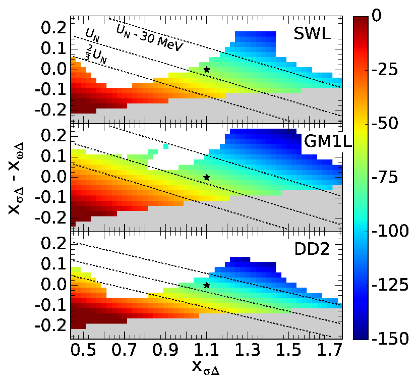In particular, we find that for the chosen parametrizations $\Delta$ s are largely absent when $x_{\sigma\Delta}-x_{\omega\Delta}\lesssim-0.1$ , and do

not populate at all when $x_{\sigma\Delta}-x_{\omega\Delta}<-0.2$ . A study by Zhu et al. 2016 investigated $\Delta$ s in the density-dependent relativistic Hartree-Fock (DDRHF) approach, and much of the analysis therein was conducted with $x_{\sigma\Delta}=0.8$ and $x_{\omega\Delta}=1.0$ . However, they did not account for hyperonization and our results suggest that $\Delta$ s may not even appear with the given choice of couplings, illustrating the importance of simultaneously considering hyperons. Finally, our investigation of the coupling range spanning $-0.25\lesssim x_{\sigma\Delta}-x_{\omega\Delta}\lesssim 0.25$ appears sufficient, as outside this range $\Delta$ s either do not populate or their presence results in an EOS that is erroneous due to either a negative effective baryon mass or a pressure that is not monotonically increasing. Thus, if $\Delta$ s are to appear in NS matter, $x_{\sigma\Delta}$ and $x_{\omega\Delta}$ are likely relatively close in value.

\Fref

fig:deltas-potential-heatmap indicates that an increase in either $x_{\sigma\Delta}$ or $x_{\sigma\Delta}-x_{\omega\Delta}$ results in a decrease in $U_{\Delta}$ , the potential becoming more attractive. The region between the top two contours is consistent with the potential constraint suggested by Drago et al. 2014 given in \erefeq:drago-constraint. Satisfaction of this constraint requires that $1.0\lesssim x_{\sigma\Delta}\lesssim 1.7$ in SWL and DD2, and $0.9\lesssim x_{\sigma\Delta}\lesssim 1.6$ in GM1L. Requiring that \erefeq:wehrberger-constraint be simultaneously satisfied completely excludes the bottom half of the coupling space and leaves only a limited region in the top-middle that is consistent with the constraints, this region including the previously employed couplings indicated by the star marker and given in \erefeq:meson-delta-couplings. The region between the bottom two contours is consistent with the potential constraint suggested in Kolomeitsev et al. 2017. However, if we simultaneously require the satisfaction of \erefeq:wehrberger-constraint here the SWL and DD2 parametrizations are completely excluded, and the $\Delta$ couplings are limited to a very small range in the GM1L parametrization.

The maximum mass of NSs in the $\sigma\omega\Delta$ coupling space is shown in \freffig:deltas-mass-heatmap. The maximum mass constraint is satisfied by the majority of the meson- $\Delta$ coupling space in all parametrizations, with large regions producing a maximum mass greater than that of the purely hyperonic EOS with ESC08 vector couplings indicated by the solid contours. Consequently the maximum mass constraint alone does not serve to constrain $x_{\sigma\Delta}$ and $x_{\omega\Delta}$ significantly. The highest maximum masses appear where both the $\Delta$ saturation potential is the most

attractive and the difference between the scalar and vector meson- $\Delta$ couplings is the greatest. Satisfaction of both \erefeq:wehrberger-constraint and the mass constraint requires $x_{\sigma\Delta}>1.0$ for SWL, $x_{\sigma\Delta}>0.9$ for GM1L, and $x_{\sigma\Delta}>0.975$ for DD2. Kolomeitsev et al. 2017 concluded that the most likely value for $U_{\Delta}(n_{0})\approx-50\,\mathrm{MeV}$ , and we find that the maximum mass constraint can only be satisfied with this potential provided $x_{\omega\Delta}>x_{\sigma\Delta}$ , violating \erefeq:wehrberger-constraint (Riek et al. 2009; Kolomeitsev et al. 2017).

The total number $N_{\Delta}$ of delta isobars present in a given NS model can be calculated from

\frac{dN_{\Delta}}{dr}=\frac{4\pi r^{2}}{\sqrt{1-2m(r)/r}}\sum_{\Delta}n_{\Delta}(r)\,,

(72)

which is to be solved in combination with the TOV equation that will be introduced in \srefsec:GR. $N_{\Delta}$ is given in \freffig:deltas-fraction-heatmap as a fraction of the total baryon number, $f_{\Delta}=N_{\Delta}/N_{B}$ . The $\Delta$ fraction varies considerably in the range $2\%\lesssim f_{\Delta}\lesssim 18\%$ when the $\sigma\omega\Delta$ couplings are consistent with the constraints given in \erefeq:drago-constraint and \erefeq:wehrberger-constraint. However, a quick examination of the same region in \freffig:deltas-mass-heatmap reveals that this variance in $f_{\Delta}$ has little to no effect on the maximum stellar mass. It appears that there is a $f_{\Delta}$ hot-spot that is centered in a region of the $\sigma\omega\Delta$ coupling space

inaccessible to the GM1L and DD2 EOS models, but the predictable result is that $f_{\Delta}$ increases with an increase in $x_{\sigma\Delta}-x_{\omega\Delta}$ when $x_{\sigma\Delta}\gtrsim 0.8$ . The DD2 parametrization presents with the highest $f_{\Delta}$ for the smallest difference $x_{\sigma\Delta}-x_{\omega\Delta}$ , followed by SWL and then GM1L.

The critical density $n_{\mathrm{cr}}$ for the appearance of $\Delta$ s is shown in \freffig:deltas-onset-heatmap for the $\sigma\omega\Delta$ coupling space. As long as \erefeq:wehrberger-constraint is satisfied, $\Delta$ s appear prior to the onset of hyperonization, and $n_{\mathrm{cr}}^{\mathrm{SWL}}\lesssim 2.3\,n_{0}$ , $n_{\mathrm{cr}}^{\mathrm{GM1L}}\lesssim 2.3\,n_{0}$ , and $n_{\mathrm{cr}}^{\mathrm{DD2}}\lesssim 1.9\,n_{0}$ . If we also enforce simultaneous satisfaction of \erefeq:drago-constraint the critical densities could be as low as $n_{\mathrm{cr}}^{\mathrm{SWL}}\approx 2\,n_{0}$ , $n_{\mathrm{cr}}^{\mathrm{GM1L}}\approx 1.9\,n_{0}$ , and $n_{\mathrm{cr}}^{\mathrm{DD2}}\approx 1.6\,n_{0}$ . Increasing $x_{\sigma\Delta}$ leads to a gradual decrease in $n_{\mathrm{cr}}$ when $x_{\sigma\Delta}-x_{\omega\Delta}\gtrsim-0.1$ , and a gradual increase in $n_{\mathrm{cr}}$ when $x_{\sigma\Delta}-x_{\omega\Delta}\lesssim-0.1$ , the increase in the repulsive vector coupling overcoming the increasingly attractive potential in the latter case. However, increasing $x_{\sigma\Delta}-x_{\omega\Delta}$ leads to an obvious and rapid decrease in $n_{c}$ for the entire $\sigma\omega\Delta$ coupling space, and if \erefeq:wehrberger-constraint is simultaneously satisfied an increase in $x_{\sigma\Delta}-x_{\omega\Delta}$ also leads to a significant reduction in the radius of the canonical $1.4\,M_{\odot}$ NS as shown in \freffig:deltas-radius-heatmap. For example, the DD2 parametrization with nucleons (and hyperons) produces a 13.5 km radius for

the canonical $1.4\,M_{\odot}$ NS and thus fails to satisfy the 13.2 km upper-radial constraint from Lattimer and Steiner 2014, but if $\Delta$ s are included and $x_{\sigma\Delta}>x_{\omega\Delta}$ the radius is reduced sufficiently to satisfy the constraint. If we allow \erefeq:drago-constraint to be violated resulting in a very attractive $U_{\Delta}$ , the inclusion of $\Delta$ s makes it possible for all three parametrizations to satisfy at least part of the $2\sigma$ upper limit on the radial constraints from Steiner et al. 2010.

5.3.2 The $x_{\rho\Delta}$ Coupling

To examine the dependence of the NS mass, the $\Delta$ critical density $n_{\mathrm{cr}}$ , and the $\Delta$ fraction $f_{\Delta}$ on the isovector meson- $\Delta$ coupling $x_{\rho\Delta}$ we set $x_{\sigma\Delta}=x_{\omega\Delta}=1.1$ and varied $x_{\rho\Delta}$ in the range $0.5<x_{\rho\Delta}<2.5$ (Spinella 2017). (Note that the saturation potential of the $\Delta$ is determined in symmetric nuclear matter and is therefore independent of $x_{\rho\Delta}$ .) The NS maximum mass was found to not be terribly sensitive to $x_{\rho\Delta}$ , decreasing over the entire range by less than $1\%$ for the GM1L and DD2 parametrizations. However, $n_{\mathrm{cr}}$ and $f_{\Delta}$ turned out to be much more sensitive to changes in $x_{\rho\Delta}$ for the GM1L parametrization due to the fact that the isovector contribution to the chemical potential is much higher than for DD2. The critical density for GM1L increases from $\sim 2\,n_{0}$ to $\sim 3\,n_{0}$ across the entire $x_{\rho\Delta}$ range, with a corresponding drop in $f_{\Delta}$ of $\sim 8-9\%$ as this EOS reverts back to a nearly purely hyperonic EOS. The $n_{\mathrm{cr}}$ of the DD2 parametrization increases very little from around $1.7\,n_{0}$ to $1.9\,n_{0}$ , but with an accompanying drop in $f_{\Delta}$ of almost 3% down to about 8%. Overall, lower values of $x_{\rho\Delta}$ lead to a lower critical density, resulting in higher fractions of $\Delta$ s to replace hyperons and lower the strangeness fraction, increasing the NS maximum mass.

6 General Relativistic Stellar Structure Equations

Neutron stars are objects of highly compressed matter so that the geometry of surrounding space-time is changed considerably from flat space. Einstein’s theory of general relativity is therefore to be used when modeling the properties of NSs rather than Newtonian mechanics. Einstein’s field equation is given by (we use units where the gravitational constant and the speed of light are $G=c=1$ )

\displaystyle R^{\mu\nu}-\frac{1}{2}g^{\mu\nu}R=8\pi T^{\mu\nu}\,,

(73)

where $R^{\mu\nu}$ is the Ricci tensor, $g^{\mu\nu}$ the metric tensor, $R$ the scalar curvature, and $T^{\mu\nu}$ the energy-momentum tensor of matter. The latter is given by

\displaystyle T^{\mu\nu}=\left(\epsilon+P(\epsilon)\right)u^{\mu}u^{\nu}+g^{\mu\nu}P(\epsilon)\,.

(74)

Models for the EOS, $P(\epsilon)$ , which are input quantities in the energy-momentum tensor equation, have been derived in \srefsec:eos. These models will be used in this section to study the properties of NSs.

6.1 Non-rotating Proto-Neutron Stars

We begin with non-rotating, spherically symmetric NSs. They are relatively easy to study since the metric of such objects depends only on the radial coordinate. The line element $ds^{2}$ in this case is given by the Schwarzschild metric (Schwarzschild 1916; Misner et al. 1973; Shapiro and Teukolsky 2008)

\displaystyle ds^{2}=-{\rm e}^{2\,\Phi(r)}dt^{2}+{\rm e}^{2\,\Lambda(r)}dr^{2}+r^{2}\,(d\theta^{2}+{\rm sin}^{2}\theta\,d\phi^{2})\,,

(75)

where $\Phi(r)$ and $\Lambda(r)$ denote unknown metric functions whose mathematical form is determined by Einstein’s field equation \erefeq:einstein and the conservation of energy-momentum, $\nabla_{\mu}T^{\mu\nu}=0$ , and have the form

	$\displaystyle{\rm e}^{2\,\Lambda(r)}$	$\displaystyle=$	$\displaystyle\left(1-\frac{2m(r)}{r}\right)^{-1}\quad({\rm inside~and~outside~of~star)}\,,$		(76)
	$\displaystyle{\rm e}^{2\,\Phi(r)}$	$\displaystyle=$	$\displaystyle\left(1-\frac{2m(r)}{r}\right)\qquad\;({\rm only~outside~of~star})\,.$		(77)

The solution of $\Phi(r)$ for the stellar interior is given by

\displaystyle\frac{d\Phi(r)}{dr}=-\frac{1}{\epsilon+P(\epsilon)}\frac{dP(r)}{dr}\,,

(78)

where the pressure gradient is given by the Tolman-Oppenheimer-Volkoff (TOV) equation (Oppenheimer and Volkoff 1939; Tolman 1939; Misner et al. 1973),

\displaystyle\frac{dP}{dr}=-\,\frac{\left(\epsilon(r)+P(r)\right)\,\left(m(r)+4\pi r^{3}P(r)\right)}{r^{2}\left(1-2m(r)/r\right)}\,.

(79)

The quantity $m(r)$ in \erefeq:TOV denotes the gravitational stellar mass given by

\displaystyle m(r)=4\pi\int_{0}^{r}\!dr\;r^{2}\,\epsilon(r)\,.

(80)

The boundary condition associated with \erefeq:TOV specifies the pressure at the stellar center, $P(r=0)$ . \Erefeq:TOV is integrated, for a given EOS, outward to a radial distance where the pressure vanishes (turns negative). This defines the radius, $R$ , of the stellar model and the star’s total gravitational mass is then given by $M\equiv m(R)$ . Figures 29 and 29 show $M$ as a function of $R$ of proto-neutron stars computed for the

DD2 and GM1L models for the nuclear EOS. The most massive stars of our sample are those with an entropy per baryon of $s=1$ and a lepton fraction of $Y_{L}=0.4$ , since the matter in their cores provides the most pressure (see Figs. 3 and 3) of all the entropy–lepton number combinations investigated in this work. The EOS computed for $s=2$ and $Y_{\nu_{e}}=0$ provides the least amount of pressure (i.e., is the softest EOS of our collection) and therefore leads to the least massive stars. We note that the mass-radius curves of all stars lighter than $\sim 1\,M_{\odot}$ are not reliable since temperature effects on the matter of the stellar crust have not been taken into account in our calculations.

6.2 Rotating Proto-Neutron Stars

The properties of rotating compact objects are much more complicated to study than those of non-rotating compact objects. This has its origin in the fact that due to rotation the stars are deformed (so that the metric functions depend on the polar angle $\theta$ ) as well as the dragging of the local inertial frames, which is caused by rotating systems in the general theory of relativity. The line element accounting for these effects is given by (Butterworth and Ipser 1976; Friedman et al. 1986)

	$\displaystyle ds^{2}=$	$\displaystyle-$	$\displaystyle{\rm e}^{2\,\nu(r,\theta,\Omega)}\,dt^{2}+{\rm e}^{2\,\psi(r,\theta,\Omega)}\,(d\phi-\omega(r,\Omega)\,dt)^{2}+{\rm e}^{2\,\mu(r,\theta,\Omega)}\,d\theta^{2}$		(81)
		$\displaystyle+$	$\displaystyle{\rm e}^{2\,\lambda(r,\theta,\Omega)}\,dr^{2}\,.$		(81)

Here, $\omega$ is the angular frequency of the local inertial frames which depends on the radial coordinate, $r$ , and on the star’s rotational frequency $\Omega$ . We take $\Omega$ to be constant throughout the star’s fluid (rigid-body rotation). Of particular interest in the discussion of rotating compact objects is the effective angular frequency $\bar{\omega}\equiv\Omega-\omega$ , which is the angular frequency of the stellar fluid relative to the local inertial frames.

6.2.1 The General Relativistic Kepler Frequency

No simple stability criteria are known for rotating star configurations in general relativity. An absolute upper limit on rapid rotation, is however set by the Kepler frequency $\Omega_{\rm K}$ , at which mass shedding from a star’s equator sets in. The expression of the general relativistic Kepler frequency is derived from the line element shown in \erefeq:metric.rot, evaluated at the equator of a compact stellar object. Since $dr=0$ and $d\theta=0$ for a mass element rotating at the equator, one obtains from \erefeq:metric.rot for the proper time $d\tau^{2}$ $(=-ds^{2})$ the relation

\displaystyle d\tau=\bigl({\rm e}^{2\,\nu(r,\theta,\Omega)}-{\rm e}^{2\,\psi(r,\theta,\Omega)}\,(\Omega-\omega(r,\theta,\Omega))^{2}\bigr)^{1/2}\,dt\,.

(82)

The equatorial orbit, which is the circular path with the maximum possible distance from the center of a gravitating body, is obtained from \erefeq:12.1bk by determining the extremum of the functional $J(r)$ associated with \erefeq:12.1bk, that is,

\displaystyle J(r)\equiv\int dt\;\bigl({\rm e}^{2\,\nu(r,\theta,\Omega)}-{\rm e}^{2\,\psi(r,\theta,\Omega)}\,(\Omega-\omega(r,\theta,\Omega))^{2}\bigr)^{1/2}\,.

(83)

Applying the extremal condition $\delta J(r)=0$ to this functional leads to

\displaystyle\delta\int dt\;\bigl({\rm e}^{2\,\nu(r,\theta,\Omega)}-{\rm e}^{2\,\psi(r,\theta,\Omega)}\,(\Omega-\omega(r,\theta,\Omega))^{2}\bigr)^{1/2}=0\,,

(84)

from which it follows that (Weber 1999)

\int dt\,\delta r\;\frac{\nu_{,r}\,{\rm e}^{2\,\nu}-\left(\psi_{,r}\,(\Omega-\omega)-\omega_{,r}\right)(\Omega-\omega)\,{\rm e}^{2\,\psi}}{\bigl({\rm e}^{2\,\nu}-{\rm e}^{2\,\psi}(\Omega-\omega)^{2}\bigr)^{1/2}}=0\,.

(85)

For the sake of brevity, we suppress all arguments here and in the following. The subscripts _,r on the metric functions and the frame dragging frequency in \erefeq:12.5bk denote partial derivatives with respect to the radial coordinate, $r$ . Next, we introduce the orbital velocity $V$ of a co-moving observer at the star’s equator relative to a locally non-rotating observer with zero angular momentum in the $\phi$ -direction. This velocity is given by

V={\rm e}^{\psi-\nu}\,(\Omega-\omega)\,.

(86)

This relation is suggested by the expression of the time-like component $u^{t}$ of the four-velocity of a mass element rotating in the equatorial plane,

\displaystyle u^{t}=\frac{dt}{d\tau}={\rm e}^{-\nu}\;\left(1-V^{2}\right)^{-1/2}\,,

(87)

where $V$ is given by \erefeq:Veq. Substituting \erefeq:Veq1 into \erefeq:12.5bk then leads to

\displaystyle{\psi_{,r}}\,{\rm e}^{2\,\nu}\,V^{2}-{\omega_{,r}}\,{\rm e}^{\nu+\psi}\,V-{\nu_{,r}}\,{\rm e}^{2\,\nu}=0\,,

(88)

which guarantees that the integrand in \erefeq:12.5bk vanishes identically for arbitrary variations $\delta r$ . \Erefeq:12.6bk represents a quadratic equation for the velocity $V$ . The solutions are given by (Friedman et al. 1986)

\displaystyle V=\frac{\omega_{,r}}{2\,\psi_{,r}}\,{\rm e}^{\psi-\nu}\pm\biggl(\frac{\nu_{,r}}{\psi_{,r}}+\biggl(\frac{\omega_{,r}}{2\,\psi_{,r}}\,{\rm e}^{2(\psi-\nu)}\biggr)^{2}\biggr)^{1/2}\,.

(89)

The general relativistic Kepler frequency, $\Omega_{\rm K}$ , is then obtained from (cf. \erefeq:Veq1) as

\displaystyle\Omega_{\rm K}={\rm e}^{\nu-\psi}\,V+\omega\,.

(90)

We note that Eqs. (89) and (90) need to be computed self-consistently together with Einstein’s field equations, which determined the metric functions $\nu$ and $\psi$ and the frame dragging frequency $\omega$ at an (initially unknown) equatorial distance. The result of classical Newtonian mechanics for the Kepler frequency and the velocity of a particle in a circular orbit, $\Omega_{\rm K}=\sqrt{M/R^{3}}$ and $V=R\Omega$ respectively, are recovered from Eqs. (89) and (90) by neglecting the curvature of space-time geometry, the rotational deformation of a rotating star, and the dragging effect of the local inertial frames.

\Fref

fig:Mass_Density_GM1L shows the impact of rapid rotation on the gravitational masses of

proto-neutron stars. The solid lines in this figure show the masses of non-rotating (i.e., TOV) stars. The dashed lines reveal by how much these masses increase if the stars are rotating at the highest possible spin rate, which is the Kepler frequency given by (90). The increase in mass of cold NSs is typically at the 20% level, depending on the EOS (Friedman et al. 1986). The same is the case for the gravitational masses of proto-neutron stars, as can be inferred from \freffig:Mass_Density_GM1L. We also note that the stars’ central energy density, $\epsilon_{c}$ , decreases with rotation speed, because of the additional rotational pressure in the radial outward direction created by rotation.

As mentioned just above, to find the Kepler frequency $\Omega_{\rm K}$ (Kepler period, $P=2\pi/\Omega_{\rm K}$ ) of a compact star, Eqs. (89) and (90) and are to be computed self-consistently in combination with the differential equations for the metric and frame-dragging functions in \erefeq:metric.rot, which follow from Einstein’s field equation (73). The entire set of coupled equations is to be evaluated at the equator of the rotating star (Friedman et al. 1986; Weber and Glendenning 1992), which is not known at the beginning of the computational procedure. Here, the results of stars rotating at the Kepler period are computed in the framework of Hartle’s perturbative rotation formalism (Weber and Glendenning 1992). The latter constitute a perturbative approach to Einstein’s field equations, that leads to results that are in very good agreement with those obtained by numerically exact treatments of Einstein’s field equations. This is particularly the case for the mass increase due to fast rotation and the value of the Kepler frequency.

\Fref

fig:MvsV_GM1L shows that the maximum possible rotational (Kepler) speed at the equator of PNSs is around $0.7\,c$ . This value depends only mildly on the actual stellar composition. One also sees that the hottest of the three stellar families (green line) terminates (solid black dot) at an equatorial speed that is smaller than the speed of the other two sequences. This has its origin in the fact that $s=2$ and $Y_{\nu_{e}}=0$ PNSs have the highest temperatures of all three configurations and thus the biggest radii, so that mass-shedding from the equator sets in first in these stars.

The Kepler periods of the rotating PNSs of Figs. 30 through 32 are displayed in \freffig:PvsM_GM1L. Based on the results shown in this figure, we conclude that PNSs posses about the same Kepler periods

as cold neutron stars.

6.2.2 Gravitational Radiation-Reaction Driven Instabilities

Besides the absolute upper limit on rapid rotation set by the Kepler frequency, there are other instabilities that have been shown to set in at a lower rotational frequency, and which therefore set more stringent limits on stable rotation (Lindblom 1986; Owen et al. 1998; Andersson et al. 1999; Andersson and Kokkotas 2001; Lin et al. 2021). They typically originate from counter-rotating surface vibrational modes, which at sufficiently high rotational star frequencies are dragged forward. In this case, gravitational radiation which inevitably accompanies the aspherical transport of matter does not damp the modes, but rather drives them (Chandrasekhar 1970; Friedman 1983b; Friedman 1983a). Bulk and shear viscosity play the important role of damping such gravitational-wave radiation-reaction instabilities at a sufficiently reduced rotational frequency such that the viscous damping rates and power in gravity waves are comparable (Lindblom and Detweiler 1977; Andersson and Kokkotas 2001). Theoretical studies suggest that either the $f$ -modes or the $r$ -modes determine the maximum rotation frequency of neutron stars.

6.3 The Moment of Inertia

Another very important stellar quantity, which will be discussed in this section, is the moment of inertia, $I$ . This quantity is given by Hartle 1973

\displaystyle I(\Omega)=\frac{1}{\Omega}\int_{A}\!\!dr\,d\theta\,d\phi\;T_{\,\phi}{{}^{t}}(r,\theta,\phi;\Omega)\,\left(-g(r,\theta,\phi;\Omega)\right)^{1/2}\,,

(91)

where $A$ denotes the region inside of a compact stellar object rotating at a uniform angular velocity, $\Omega$ . The quantity $g$ denotes the determinant of the metric tensor $g_{\mu\nu}$ , whose components can be read off from \erefeq:metric.rot. One obtains (Weber 1999)

\sqrt{-g}={\rm e}^{\lambda+\mu+\nu+\psi}\,.

(92)

The energy-momentum tensor component $T_{\phi}{}^{t}$ is given by (see \erefeq:Tmunu.GR)

T_{\phi}{}^{t}=(\epsilon+P)\;u_{\phi}\,u^{t}\,,

(93)

with the four-velocities $u_{\phi}$ and $u^{t}$ given by

	$\displaystyle u^{t}$	$\displaystyle=$	$\displaystyle\frac{{\rm e}^{-\nu}}{\left(1-(\omega-\Omega)^{2}\,{\rm e}^{2\psi-2\nu}\right)^{1/2}}\,,$		(94)
	$\displaystyle u_{\phi}$	$\displaystyle=$	$\displaystyle(\Omega-\omega)\;{\rm e}^{2\,\psi}\;u^{t}\,.$		(95)

Substituting Eqs. (94) and (95) into \erefeq:11.TPt leads for $T_{\phi}{}^{t}$ to

\displaystyle T_{\phi}{}^{t}=\frac{(\epsilon+P)\,(\Omega-\omega)\,{\rm e}^{2\,\psi}}{{\rm e}^{2\,\nu}-(\omega-\Omega)^{2}\,{\rm e}^{2\,\psi}}\,.

(96)

Substituting the expression given in \erefeq:minusg and \erefeq:11.70bk into \erefeq:11.64bk leads for the moment of inertia of a rotationally deformed compact stellar object to (Weber 1999)

\displaystyle I(\Omega)=2\pi\!\int_{0}^{\pi}\!d\theta\int_{0}^{R(\theta)}\!\!dr\,{\rm e}^{\lambda+\mu+\nu+\psi}\,\frac{\epsilon+P(\epsilon)}{{\rm e}^{2\nu-2\psi}-(\omega-\Omega)^{2}}\,\frac{\Omega-\omega}{\Omega}\,.

(97)

In Figs. 34 and 34 we show the results for the moment of inertia computed for the DD2 and GM1L nuclear parametrizations.

As can be seen, massive PNSs with $s=1$ and $Y_{L}=0.4$ posses the largest moments of inertia, followed by PNS with $s=2$ and $Y_{L}=0.2$ , and $s=2$ and $Y_{\nu_{e}}=0.0$ . This trend is consistent with the stiffness of the PNS equations of state shown in Figs. 3 through 5, the associated mass-radius relationships shown in Figs. 29 and 29, and the mass-central density curves shown \freffig:Mass_Density_GM1L. Figures 34 and 34 show that $2\,M_{\odot}$ PNSs, for instance, possess moments of inertia of around 270 km³. It is interesting to compare this value with the moment of inertia of a spherical uniform mass distribution in Newtonian physics, which is given by $I=\frac{2}{5}MR^{2}=\frac{3}{5}(\frac{M}{M_{\odot}})(\frac{R}{\rm km})^{2}~{\rm km}^{3}$ . This gives values for $I$ for the $2\,M_{\odot}$ PNSs in Figs. 29 and 29 which are between 175 km³ and 235 km³. These values are on the same order of magnitude as the general relativistic results, but differ significantly quantitatively. Sudden changes $\Delta I$ in the moments of inertia of (proto-) neutron stars are expected to lead to sudden changes $\Delta\Omega$ in the spin frequencies of such objects. Assuming angular momentum conservation during such episodes, the change in spin frequency may be estimated as

\frac{\Delta\Omega}{\Omega}=-\frac{\Delta I}{I+\Delta I}\,,

(98)

where $\Omega$ is the frequency of the star before the change in the moment of inertia. Observed changes in the spin frequencies of rotating neutron stars (pulsars) range from $10^{-6}$ to $10^{-9}$ and have been suggested to originate from sudden decreases in the moments of inertia of such objects (Lyne 1992; Fuentes, J. R. et al. 2017; Manchester 2017; Montoli et al. 2022). Similar arguments have been used by Garcia and Ranea-Sandoval 2015 and Mastrano et al. 2015 to explain the anti-glitch observed for the magnetar AXP 1E 2259+586 Archibald et al. 2013. \Erefeq:delOmega indicates that already $|\Delta I|\sim 10^{-6}$ km³ to $10^{-9}$ km³ could suffice to cause such changes. This is also the reason why the nuclear crust on hypothetical strange quark stars could explain the observed pulsar glitches Glendenning and Weber 1992.

7 Future Directions of Research

It is often stressed that there has never been a more exciting time in the overlapping areas of nuclear physics, particle physics, relativistic astrophysics and astronomy than today. This interest is stimulated by investments made in international nuclear physics facilities such as FAIR, FRIB, NICA, CERN, BNL, J-Park and multiple new instruments for sky surveys that have become operational in recent years, such as FAST, eROSITA, NICER and the gravitational-wave detectors LIGO, VIRGO, KAGRA. In particular, the observation of the first binary neutron star merger, GW170817, using LIGO and VIRGO (Abbott 2017) have led the scientific community into the new era named multi-messenger astronomy with gravitational waves.

Depending on the combined masses of two merging NSs, there are in principle four possible outcomes to a merger (Chirenti et al. 2019): 1) prompt formation of a black hole, 2) formation of a hypermassive NS (HMNS) (Baumgarte et al. 2000; Shapiro 2000), 3) formation of a supramassive rotating NS (Falcke and Rezzolla 2014), or 4) the formation of a stable NS. Numerical relativity simulations have shown that the threshold masses related to these scenarios depend strongly on the properties and the EOS of hot and dense NS matter. (For a comprehensive review of the physics of NS mergers, see Baiotti and Rezzolla 2017, and references therein.) The same is true for the lifetime of HMNSs, which depends strongly on the total mass of the binary system and, thus, on the nuclear EOS. The post-merger emissions are typically characterized by two distinct frequency peaks, one at high and the other at lower frequencies. The EOS dependent high-frequency peak is believed to be associated with the oscillations of the HMNS produced in a merger, while the low-frequency peak is understood to be related to the merger process and to the total compactness (i.e., mass-radius ratio) of the merging objects (Takami et al. 2015), which is inexorably linked to the EOS of dense nuclear matter.

The EOS of cold and dense nuclear matter is sufficient to describe NS matter prior to a NS merger. After contact, however, large shocks develop which considerably increase the internal energy of the colliding NSs. Numerical simulations have shown that overall matter in NS collisions reaches densities that are several times higher than the nuclear saturation density and temperatures that are roughly as high as 50 MeV (Baiotti and Rezzolla 2017; Hanauske et al. 2019a; Perego, Albino et al. 2019). As shown in this chapter, such extreme conditions of density and pressure modify the EOS and in particular the baryon-lepton composition of the matter tremendously.

Very recently, is has been shown that a strong first-order phase transition in NS mergers may register itself in the gravitational-wave frequency, $f_{\rm peak}$ , and the stellar tidal deformability, $\Lambda$ Bauswein et al. 2019. Since both the tidal deformability during inspiral and the oscillation frequencies of the post-merger remnant can be determined very reliably Faber and Rasio 2012; Baiotti and Rezzolla 2017; Paschalidis and Stergioulas 2017; Friedman 2018; Duez and Zlochower 2018, this finding relates NS merger simulations to the general science question whether or not phase transitions occur in dense nuclear matter. Signatures of possible hadron-quark phase transitions in NS mergers have also been studied by Most et al. 2019. This study shows that changes in the pressure of the quark phase can produce a decisive signature in the post-merger gravitational-wave signal and spectrum. It was also shown that a hadron-quark phase transition may lead to a hot and dense quark core which could produce a ring-down signal different from what is expected for a pure hadronic core. The possibility of detecting the hadron-quark phase transition with gravitational waves has been discussed recently by Hanauske et al. 2019b.

A great deal of experimental, theoretical as well as computational work will need to be carried out over the coming years to determine a comprehensive class of state-of-the-art models for the EOS of ultra-hot and dense nuclear matter for use in binary NS merger simulations and PNS simulations (Shen et al. 2011; Rezzolla and Olindo 2013; Banik et al. 2014; Hanauske et al. 2019b).

Acknowledgments

This research was supported by the National Science Foundation (USA) under Grants No. PHY-1714068 and PHY-2012152. MO and IFR-S thank CONICET, UNLP, and MinCyT (Argentina) for financial support under grants PIP-0714, G157, G007 and PICT 2019-3662. The results of this paper contribute to the research projects of the NP3M collaboration on the Nuclear Physics of Multi-Messenger Mergers.

References

Abbott (2017) Abbott, B. P. et al.. (2017). GW170817: Observation of gravitational waves from a binary neutron star inspiral, Phys. Rev. Lett. 119, pp. 161101.
Alford et al. (2001) Alford, M., Rajagopal, K., Reddy, S., Wilczek, F. (2001). Minimal color-flavor-locked-nuclear interface, Phys. Rev. D 64, p. 074017.
Alford et al. (2008) Alford, M. G., Schmitt, A., Rajagopal, K., and Schäfer, T. (2008). Color superconductivity in dense quark matter, Rev. Mod. Phys. 80, pp. 1455–1515.
Andersson et al. (1999) Andersson, N., Kokkotas, K., and Schutz, B. F. (1999). Gravitational radiation limit on the spin of young neutron stars, Astrophys. J. 510, 2, pp. 846–853.
Andersson and Kokkotas (2001) Andersson, N. and Kokkotas, K. D. (2001). The r-mode instability in rotating neutron stars, Int. J. Mod. Phys. D 10, pp. 381–441.
Antoniadis et al. (2013) Antoniadis, J. et al. (2013). A Massive Pulsar in a Compact Relativistic Binary, Science 340, pp. 6131.
Archibald et al. (2013) Archibald, R. F. et al. (2013). An anti-glitch in a magnetar. Nature 497, pp. 591–-593.
Arzoumanian et al. (2018) Arzoumanian, Z., Brazier, A., Burke-Spolaor, S., Chamberlin, S., Chatterjee, S., Christy, B., Cordes, J. M., Cornish, N. J., Crawford, F., Cromartie, H. T., Crowter, K., DeCesar, M. E., Demorest, P. B., Dolch, T., Ellis, J. A., Ferdman, R. D., Ferrara, E. C., Fonseca, E., Garver-Daniels, N., Gentile, P. A., Halmrast, D., Huerta, E. A., Jenet, F. A., Jessup, C., Jones, G., Jones, M. L., Kaplan, D. L., Lam, M. T., Lazio, T. J. W., Levin, L., Lommen, A., Lorimer, D. R., Luo, J., Lynch, R. S., Madison, D., Matthews, A. M., McLaughlin, M. A., McWilliams, S. T., Mingarelli, C., Ng, C., Nice, D. J., Pennucci, T. T., Ransom, S. M., Ray, P. S., Siemens, X., Simon, J., Spiewak, R., Stairs, I. H., Stinebring, D. R., Stovall, K., Swiggum, J. K., Taylor, S. R., Vallisneri, M., van Haasteren, R., Vigeland, S. J., and and, W. Z. (2018). The NANOGrav 11-year data set: High-precision timing of 45 millisecond pulsars, The Astrophys. J. Suppl. Ser. 235, 2, pp. 37.
Baiotti and Rezzolla (2017) Baiotti, L. and Rezzolla, L. (2017). Binary neutron star mergers: a review of einstein’s richest laboratory, Reports on Progress in Physics 80, 9, pp. 096901.
Banik et al. (2014) Banik, S., Hempel, M., and Bandyopadhyay, D. (2014). New Hyperon Equations of State for Supernovae and Neutron Stars in Density-Dependent Hadron Field Theory, Astrophys. J. Suppl. Ser. 214, 2, p. 22.
Baumgarte et al. (2000) Baumgarte, T. W., Shapiro, S. L., and Shibata, M. (2000). On the maximum mass of differentially rotating neutron stars, Astrophys. J. 528, 1, pp. L29–L32.
Bauswein et al. (2019) Bauswein, A., Bastian, N.-U. F., Blaschke, D. B., Chatziioannou, K., Clark, J. A., Fischer, T., and Oertel, M. (2019). Identifying a first-order phase transition in neutron-star mergers through gravitational waves, Phys. Rev. Lett. 122, p. 061102.
Baym and Chin (1976) Baym, G. and Chin, S. (1976). Can a neutron star be a giant mit bag? Physics Letters B 62, 2, pp. 241–244.
Baym, et al. (2018) Baym, Gordon and Hatsuda, Tetsuo and Kojo, Toru and Powell, Philip D. and Song, Yifan and Takatsuka, Tatsuyuki (2018). From hadrons to quarks in neutron stars: a review, Rept. Prog. Phys. 81, 5, pp. 056902.
Becker (2009) Becker, W. (2009). Neutron Stars and Pulsars, Astrophysics and Space Science Library (Springer, Berlin Heidelberg).
Blaschke and Chamel (2018) Blaschke, D. and Chamel, N. (2018). Phases of Dense Matter in Compact Stars (Springer International Publishing, Cham), ISBN 978-3-319-97616-7, pp. 337–400.
Boguta (1982) Boguta, J. (1982). Baryonic degrees of freedom leading to density isomers, Phys. Lett. B 109, 4, pp. 251–254.
Boguta and Bodmer (1977) Boguta, J. and Bodmer, A. R. (1977). Relativistic calculation of nuclear matter and the nuclear surface, Nucl. Phys. A 292, pp. 413.
Bonanno, Luca and Sedrakian, Armen (2012) Bonanno, Luca and Sedrakian, Armen (2012). Composition and stability of hybrid stars with hyperons and quark color-superconductivity, A&A 539, pp. A16.
Buballa (2005) Buballa, M. (2005). Njl-model analysis of dense quark matter, Phys. Rept. 407, 4-6, pp. 205–376.
Burgio and Plumari (2008) Burgio, G. and Plumari, S. (2008). Structure of hybrid protoneutron stars within the nambu-jona-lasinio model, Phys. Rev. D 77, 8, pp. 085022.
Burrows and Vartanyan (2021) Burrows, A. and Vartanyan, D. (2021). Core-collapse supernova explosion theory, Nature 589, pp. 29–39.
Butterworth and Ipser (1976) Butterworth, E. M. and Ipser, J. R. (1976). On the structure and stability of rapidly rotating fluid bodies in general relativity. I. The numerical method for computing structure and its application to uniformly rotating homogeneous bodies. Astrophys. J. 204, pp. 200–223.
Cai et al. (2015) Cai, B.-J., Fattoyev, F. J., Li, B.-A., and Newton, W. G. (2015). Critical density and impact of $\mathrm{\Delta}(1232)$ resonance formation in neutron stars, Phys. Rev. C 92, pp. 015802.
Camelio et al. (2017) Camelio, G., Lovato, A., Gualtieri, L., Benhar, O., Pons, J., and Ferrari, V. (2017). Evolution of a proto-neutron star with a nuclear many-body equation of state: Neutrino luminosity and gravitational wave frequencies, Phys. Rev. D 96, pp. 043015.
Chandrasekhar (1970) Chandrasekhar, S. (1970). Solutions of two problems in the theory of gravitational radiation, Phys. Rev. Lett. 24, pp. 611–615.
Chapline and Nauenberg (1977) Chapline, G. and Nauenberg, M. (1977). Asymptotic freedom and the baryon-quark phase transition, Phys. Rev. D 16, pp. 450–456.
Chen et al. (2009) Chen, Y., Yuan, Y., and Liu, Y. (2009). Neutrino mean free path in neutron star matter with $\Delta$ isobars, Phys. Rev. C 79, pp. 055802.
Chirenti et al. (2019) Chirenti, C., Miller, M. C., Strohmayer, T., and Camp, J. (2019). Searching for hypermassive neutron stars with short gamma-ray bursts, Astrophys. J. 884, 1, pp. L16.
Demorest et al. (2010) Demorest, P., Pennucci, T., Ransom, S., Roberts, M., and Hessels, J. (2010). Shapiro Delay Measurement of A Two Solar Mass Neutron Star, Nature 467, pp. 1081–1083.
Dexheimer and Schramm (2008) Dexheimer, V. and Schramm, S. (2008). Proto–neutron and neutron stars in a chiral SU(3) model, Astrophys. J. 683, 2, pp. 943–948.
Dolan and Jackiw (1974) Dolan, L. and Jackiw, R. (1974). Symmetry behavior at finite temperature, Phys. Rev. D 9, pp. 3320–3341.
Drago et al. (2014) Drago, A., Lavagno, A., Pagliara, G., and Pigato, D. (2014). Early appearance of $\Delta$ isobars in neutron stars, Phys. Rev. C 90, pp. 065809.
Duez and Zlochower (2018) Duez, M. D. and Zlochower, Y. (2018). Numerical relativity of compact binaries in the 21st century, Rep. Prog. Phys. 82, 1, p. 016902.
Faber and Rasio (2012) Faber, J. A. and Rasio, F. A. (2012). Binary neutron star mergers, Living Reviews in Relativity 15, 1, p. 8.
Falcke and Rezzolla (2014) Falcke, H. and Rezzolla, L. (2014). Fast radio bursts: the last sign of supramassive neutron stars, A&A 562, pp. A137.
Fechner and Joss (1978) Fechner, W. B. and Joss, P. C. (1978). Quark Stars with ’Realistic’ Equations of State, Nature 274, pp. 347–349.
Fischer et al. (2010) Fischer, T., Whitehouse, S. C., Mezzacappa, A., Thielemann, F. K., and Lienbendörfer, M. (2010). Protoneutron star evolution and the neutrino-driven wind in general relativistic neutrino radiation hydrodynamics simulations, A&A 517, pp. A80.
Foglizzo (2016) Foglizzo, T. (2016). Explosion Physics of Core-Collapse Supernovae (Springer International Publishing, Cham), pp. 1–21.
Friedman and Gal (2021) Friedman, E. and Gal, A. (2021). Constraints on ${\Xi}^{\text{--}}$ nuclear interactions from capture events in emulsion, Phys. Lett. B 820, pp. 136555.
Friedman (1983a) Friedman, J. L. (1983a). Upper limit on the frequency of fast pulsars, Phys. Rev. Lett. 51, pp. 718–718.
Friedman (1983b) Friedman, J. L. (1983b). Upper limit on the frequency of pulsars, Phys. Rev. Lett. 51, pp. 11–14.
Friedman (2018) Friedman, J. L. (2018). Gravitational-wave astrophysics from neutron star inspiral and coalescence, Int. J. Mod. Phys. D 27, 11, 1843018.
Friedman et al. (1986) Friedman, J. L., Ipser, J. R., and Parker, L. (1986). Rapidly Rotating Neutron Star Models, Astrophys. J. 304, pp. 115.
Fritzsch et al. (1973) Fritzsch, H., Gell-Mann, M., and Leutwyler, H. (1973). Advantages of the color octet gluon picture, Physics Letters B 47, 4, pp. 365–368.
Fuchs et al. (1995) Fuchs, C., Lenske, H., and Wolter, H. H. (1995). Density dependent hadron field theory, Phys. Rev. C 52, pp. 3043–3060.
Fuentes, J. R. et al. (2017) Fuentes, J. R., Espinoza, C. M., Reisenegger, A., Shaw, B., Stappers, B. W., and Lyne, A. G. (2017). The glitch activity of neutron stars, A&A 608, p. A131.
Fukushima and Hatsuda (2011) Fukushima, K. and Hatsuda, T. (2011). The phase diagram of dense QCD, Rept. Prog. Phys. 74, pp. 014001.
Fukushima and Sasaki (2013) Fukushima, K. and Sasaki, C. (2013). The phase diagram of nuclear and quark matter at high baryon density, Prog. Part. Nucl. Phys. 72, pp. 99–154.
Garcia and Ranea-Sandoval (2015) Garcia, F., Ranea-Sandoval, I. F. (2015). A simple mechanism for the anti-glitch observed in AXP 1E 2259+586. Mon. Not. R. Astron. Soc. 449, pp. L73–L76.
Glendenning (2012) Glendenning, N. K. (2012). Compact Stars: Nuclear Physics, Particle Physics and General Relativity, Astronomy and Astrophysics Library (Springer, New York).
Glendenning (1985) Glendenning, N. K. (1985). Neutron stars are giant hypernuclei?, Astrophys. J. 293, pp. 470–493.
Glendenning and Weber (1992) Glendenning, N. K. and Weber, F. (1992). Nuclear Solid Crust on Rotating Strange Quark Stars, Astrophys. J. 400, p. 647.
Hanauske et al. (2019a) Hanauske, M., Bovard, L., Most, E., Papenfort, J., Steinheimer, J., Motornenko, A., Vovchenko, V., Dexheimer, V., Schramm, S., and Stöcker, H. (2019a). Detecting the hadron-quark phase transition with gravitational waves, Universe 5, 6.
Hanauske et al. (2019b) Hanauske, M., Steinheimer, J., Motornenko, A., Vovchenko, V., Bovard, L., Most, E. R., Papenfort, L. J., Schramm, S., and Stöcker, H. (2019b). Neutron star mergers: Probing the eos of hot, dense matter by gravitational waves, Particles 2, 1, pp. 44–56.
Hartle (1973) Hartle, J. (1973). Slowly Rotating Relativistic Stars. IX: Moments of Inertia of Rotationally Distorted Stars, Astrophys. and Space Sci. 24, pp. 385–405.
Hatsuda and Kunihiro (1994) Hatsuda, T. and Kunihiro, T. (1994). Qcd phenomenology based on a chiral effective lagrangian, Phys. Rept. 247, 5, pp. 221–367.
Hofmann et al. (2001) Hofmann, F., Keil, C. M., and Lenske, H. (2001). Application of the density dependent hadron field theory to neutron star matter, Phys. Rev. C 64, pp. 025804.
Huber et al. (1998) Huber, H., Weber, F., Weigel, M. K., and Schaab, C. (1998). Neutron Star Properties with Relativistic Equations of State, Int. J. Mod. Phys. E 7, 3, pp. 301–339.
Hüdepohl et al. (2010) Hüdepohl, L., Müller, B., Janka, H.-T., Marek, A., and Raffelt, G. G. (2010). Neutrino signal of electron-capture supernovae from core collapse to cooling, Phys. Rev. Lett. 104, pp. 251101.
Itoh (1970) Itoh, N. (1970). Hydrostatic Equilibrium of Hypothetical Quark Stars, Prog. Theor. Phys. 44, pp. 291.
Ivanenko and Kurdgelaidze (1965) Ivanenko, D. D. and Kurdgelaidze, D. F. (1965). Hypothesis concerning quark stars, Astrophysics 1, pp. 251–252.
Janka (2012) Janka, H.-T. (2012). Explosion mechanisms of core-collapse supernovae, Ann. Rev. Nucl. Part. Sci. 62, 1, pp. 407–451.
Kajantie et al. (1991) Kajantie, K., Kärkkäinen, L., and Rummukainen, K. (1991). Tension of the interface between two ordered phases in lattice su(3) gauge theory, Nucl. Phys. B 357, 2, pp. 693–712.
Ke and Liu (2014) Ke, W. and Liu, Yu-xin (2014). Interface tension and interface entropy in the 2+1 flavor Nambu-Jona-Lasinio model, Phys. Rev. D 89, p. 074041.
Keister and Kisslinger (1976) Keister, B. and Kisslinger, L. (1976). Free-quark phases in dense stars, Phys. Lett. B 64, 1, pp. 117–120.
Klevansky (1992) Klevansky, S. P. (1992). The nambu—jona-lasinio model of quantum chromodynamics, Rev. Mod. Phys. 64, pp. 649–708.
Kolomeitsev et al. (2017) Kolomeitsev, E., Maslov, K., and Voskresensky, D. (2017). Delta isobars in relativistic mean-field models with $\sigma$ –scaled hadron masses and couplings, Nucl. Phys. A 961, pp. 106–141.
Lattimer and Steiner (2014) Lattimer, J. M. and Steiner, A. W. (2014). Constraints on the symmetry energy using the mass-radius relation of neutron stars, The Eur. Phys. J. A 50, 2, p. 40.
Lavagno (2010) Lavagno, A. (2010). Hot and dense hadronic matter in an effective mean-field approach, Phys. Rev. C 81, pp. 044909.
Li et al. (2018) Li, J. J., Sedrakian, A., and Weber, F. (2018). Competition between delta isobars and hyperons and properties of compact stars, Phys. Lett. B 783, pp. 234–240.
Lin et al. (2021) Lin, Z., Bratton, E., Weber, F., Orsaria, M. G., and Ranea-Sandoval, I. F. (2021). Gravitational radiation-reaction driven instabilities in rotating neutron stars, Astron. Nachr. 342, pp. 799–807.
Lindblom (1986) Lindblom, L. (1986). Estimates of the maximum angular velocity of rotating neutron stars, Astrophys. J. 303, pp. 146.
Lindblom and Detweiler (1977) Lindblom, L. and Detweiler, S. L. (1977). On the secular instabilities of the Maclaurin spheroids. Astrophys. J. 211, pp. 565–567.
Lugones et al. (2013) Lugones, G., Grunfeld, A. G., Ajmi, M. A. (2013). Surface tension and curvature energy of quark matter in the Nambu-Jona-Lasinio model, Phys. Rev. C 88, p. 045803.
Lynch et al. (2013) Lynch, R. S. et al. (2013). The Green Bank Telescope 350 MHz Drift-scan Survey II: Data Analysis and the Timing of 10 New Pulsars, Including a Relativistic Binary, Astrophys. J. 763, p. 81.
Lyne (1992) Lyne, A. G. (1992). Glitches as probes of neutron star interiors, Philosophical Transactions: Physical Sciences and Engineering 341, 1660, pp. 29–37.
Malfatti et al. (2019) Malfatti, G., Orsaria, M. G., Contrera, G. A., Weber, F., and Ranea-Sandoval, I. F. (2019). Hot quark matter and (proto-) neutron stars, Phys. Rev. C 100, p. 015803.
Malfatti (2020) Malfatti, G. (2020). Non-local quark models for description of dense matter in the cores of neutron stars, Ph.D. thesis, La Plata U., 10.35537/10915/107749, arXiv:2010.14728 [nucl-th].
Malfatti et al. (2020) Malfatti, G., Orsaria, M. G., Ranea-Sandoval, I. F., Contrera, G. A., and Weber, F. (2020). Delta baryons and diquark formation in the cores of neutron stars, Phys. Rev. D 102, pp. 063008.
Manchester (2017) Manchester, R. (2017). Pulsar glitches, Proceedings of the International Astronomical Union 13, pp. 197–202.
Mariani et al. (2017) Mariani, M., Orsaria, M., and Vucetich, H. (2017). Constant entropy hybrid stars: a first approximation of cooling evolution, A&A 601, pp. A21.
Mariani (2020) Mariani, M. (2020). Estrellas híbridas aisladas: criterios de estabilidad en modelos de proto-estrellas de neutrones y magnetares, Ph.D. thesis, Universidad Nacional de La Plata, Argentina.
Maslov et al. (2016) Maslov, K., Kolomeitsev, E., and Voskresensky, D. (2016). Relativistic mean-field models with scaled hadron masses and couplings: Hyperons and maximum neutron star mass, Nucl. Phys. A 950, pp. 64–109.
Mastrano et al. (2015) Mastrano, A., Suvorov, A. G., Melatos, A. (2015). Interpreting the AXP 1E 2259+586 antiglitch as a change in internal magnetization. Mon. Not. R. Astron. Soc. 453, pp. 522-–530.
Mezzacappa (2005) Mezzacappa, A. (2005). Ascertaining the core collapse supernova mechanism: The state of the art and the road ahead, Ann. Rev. Nucl. Part. Sci. 55, 1, pp. 467–515.
Misner et al. (1973) Misner, C. W., Thorne, K. S., and Wheeler, J. A. (1973). Gravitation (Freeman and Company, San Francisco).
Miyatsu et al. (2013) Miyatsu, T., Cheoun, M.-K., and Saito, K. (2013). Equation of state for neutron stars in su(3) flavor symmetry, Phys. Rev. C 88, pp. 015802.
Montoli et al. (2022) Montoli, A., Pizzochero, P. M., and Antonelli, M. (2022). Insight into the physics of neutron star interiors from pulsar glitches, Astrophysics in the XXI Century with Compact Stars (World Scientific), ISBN 978-9-811-22093-7, (in press).
Most et al. (2019) Most, E. R., Papenfort, L. J., Dexheimer, V., Hanauske, M., Schramm, S., Stöcker, H., and Rezzolla, L. (2019). Signatures of quark-hadron phase transitions in general-relativistic neutron-star mergers, Phys. Rev. Lett. 122, p. 061101.
Oertel et al. (2017) Oertel, M., Hempel, M., Klähn, T., and Typel, S. (2017). Equations of state for supernovae and compact stars, Rev. Mod. Phys. 89, p. 015007.
Oppenheimer and Volkoff (1939) Oppenheimer, J. R. and Volkoff, G. M. (1939). On massive neutron cores, Phys. Rev. 55, pp. 374–381.
Orsaria et al. (2013) Orsaria, M., Rodrigues, H., Weber, F., and Contrera, G. A. (2013). Quark-hybrid matter in the cores of massive neutron stars, Phys. Rev. D8, 2, pp. 023001.
Orsaria et al. (2014) Orsaria, M., Rodrigues, H., Weber, F., and Contrera, G. A. (2014). Quark deconfinement in high-mass neutron stars, Phys. Rev. C89, 1, pp. 015806.
Orsaria et al. (2019) Orsaria, M. G., Malfatti, G., Mariani, M., Ranea-Sandoval, I. F., García, F., Spinella, W. M., Contrera, G. A., Lugones, G., and Weber, F. (2019). Phase transitions in neutron stars and their links to gravitational waves, J. Phys. G: Nucl. Part. Phys. 46, 7, pp. 073002.
Owen et al. (1998) Owen, B. J., Lindblom, L., Cutler, C., Schutz, B. F., Vecchio, A., and Andersson, N. (1998). Gravitational waves from hot young rapidly rotating neutron stars, Phys. Rev. D 58, pp. 084020.
Page et al. (2006) Page, D., Geppert, U., and Weber, F. (2006). The cooling of compact stars, Nucl. Phys. A 777, pp. 497–530,
Page and Reddy (2006) Page, D. and Reddy, S. (2006). Dense Matter in Compact Stars: Theoretical Developments and Observational Constraints, Ann. Rev. Nucl. Part. Sci. 56, 1, pp. 327–374.
Pandharipande (1971) Pandharipande, V. (1971). Hyperonic matter, Nucl. Phys. A 178, 1, pp. 123–144.
Paschalidis and Stergioulas (2017) Paschalidis, V. and Stergioulas, N. (2017). Rotating stars in relativity, Living Reviews in Relativity 20, 1, p. 7,
Perego, Albino et al. (2019) Perego, Albino, Bernuzzi, Sebastiano, and Radice, David (2019). Thermodynamics conditions of matter in neutron star mergers, Eur. Phys. J. A 55, 8, pp. 124.
Pons et al. (1999) Pons, J. A., Reddy, S., Prakash, M., Lattimer, J. M., and Miralles, J. A. (1999). Evolution of Proto-Neutron Stars, Astrophys. J. 513, pp. 780–804.
Prakash et al. (1997) Prakash, M., Bombaci, I., Prakash, M., Ellis, P. J., Lattimer, J. M., and Knorren, R. (1997). Composition and structure of protoneutron stars, Physics Reports 280, 1, pp. 1–77.
Rezzolla and Olindo (2013) Rezzolla, L. and Olindo, Z. (2013). Relativistic Hydrodynamics (Oxford University Press).
Rezzolla et al. (2019) Rezzolla, L., Pizzochero, P., Jones, D., Rea, N., and Vidaña, I. (2019). The Physics and Astrophysics of Neutron Stars, Astrophysics and Space Science Library (Springer International Publishing).
Riek et al. (2009) Riek, F., Lutz, M. F. M., and Korpa, C. L. (2009). Photoabsorption off nuclei with self-consistent vertex corrections, Phys. Rev. C 80, pp. 024902.
Rijken et al. (2010) Rijken, T. A., Nagels, M. M., and Yamamoto, Y. (2010). Baryon-Baryon Interactions: — Nijmegen Extended-Soft-Core Models —, Prog. Theor. Phys. Suppl. 185, pp. 14–71.
Sawyer (1972) Sawyer, R. F. (1972). Energy shifts of excited nucleons in neutron-star matter, Astrophys. J. 176, pp. 205–211.
Schaffner-Bielich and Gal (2000) Schaffner-Bielich, J. and Gal, A. (2000). Properties of strange hadronic matter in bulk and in finite systems, Phys. Rev. C 62, pp. 034311.
Schürhoff et al. (2010) Schürhoff, T., Schramm, S., and Dexheimer, V. (2010). Neutron Stars with small Radii—The Role of $\delta$ Resonaces, Astrophys. J. 724, 1, pp. L74–L77.
Schwarzschild (1916) Schwarzschild, K. (1916). On the gravitational field of a sphere of incompressible fluid according to Einstein’s theory, Sitzungsber. Preuss. Akad. Wiss. Berlin (Math. Phys. ) 1916, pp. 424–434.
Sedrakian (2007) Sedrakian, A. (2007). The physics of dense hadronic matter and compact stars, Prog. Part. Nucl. Phys. 58, 1, pp. 168–246.
Sedrakian et al. (2022) Sedrakian, A., Li, J.-J., and Weber, F. (2022). Hyperonization in Compact Stars, Astrophysics in the XXI Century with Compact Stars (World Scientific), ISBN 978-9-811-22093-7, (in press).
Shao (2011) Shao, G.-Y. (2011). Evolution of proto-neutron stars with the hadron–quark phase transition, Phys. Lett. B 704, 4, pp. 343–-346.
Shapiro (2000) Shapiro, S. L. (2000). Differential rotation in neutron stars: Magnetic braking and viscous damping, Astrophys. J. 544, 1, pp. 397–408.
Shapiro and Teukolsky (2008) Shapiro, S. L. and Teukolsky, S. A. (1983). Black Holes, White Dwarfs, and Neutron Stars: The Physics of Compact Objects (Wiley).
Shen et al. (2011) Shen, G., Horowitzn, C. J., and Teige, S. (2011). A new equation of state for astrophysical simulations, Phys. Rev. C 83, pp. 035802.
Sotani et al. (2011) Sotani, H., Yasutake, N., Maruyama, T., and Tatsumi, T. (2011). Signatures of hadron-quark mixed phase in gravitational waves, Phys. Rev. D 83, p. 024014.
Spinella (2017) Spinella, W. M. (2017). A Systematic Investigation of Exotic Matter in Neutron Stars, Ph.D. thesis, Claremont Graduate University & San Diego State University.
Spinella and Weber (2020) Spinella, W. M. and Weber, F. (2020). Dense Baryonic Matter in the Cores of Neutron Stars, Topics on Strong Gravity, Chap. 4 (World Scientific), pp. 85–152.
Spinella et al. (2018) Spinella, W. M., Weber, F., Orsaria, M. G., and Contrera, G. A. (2018). Neutrino Emissivity in the Quark-Hadron Mixed Phase, Universe 4, 5, pp. 64.
Steiner et al. (2000) Steiner, A., Prakash, M., and Lattimer, J. (2000). Quark-hadron phase transitions in young and old neutron stars, Phys. Lett. B 486, 3-4, pp. 239–248.
Steiner et al. (2010) Steiner, A. W., Lattimer, J. M., and Brown, E. F. (2010). The Equation of State from Observed Masses and Radii of Neutron Stars, Astrophys. J. 722, 1, pp. 33–54.
Takami et al. (2015) Takami, K., Rezzolla, L., and Baiotti, L. (2015). Spectral properties of the post-merger gravitational-wave signal from binary neutron stars, Phys. Rev. D 91, pp. 064001.
Tolman (1939) Tolman, R. C. (1939). Static solutions of einstein’s field equations for spheres of fluid, Phys. Rev. 55, pp. 364–373.
Tolos and Fabbietti (2020) Tolos, L. and Fabbietti, L. (2020). Strangeness in nuclei and neutron stars, Prog. Part. Nucl. Phys. 112, pp. 103770.
Typel (2018) Typel, S. (2018). Relativistic Mean-Field Models with Different Parametrizations of Density Dependent Couplings, Particles 1, 1, pp. 3–22.
Typel et al. (2010a) Typel, S., Röpke, G., Klähn, T., Blaschke, D., and Wolter, H. H. (2010a). Composition and thermodynamics of nuclear matter with light clusters, Phys. Rev. C 81, pp. 015803.
Typel et al. (2010b) Typel, S., Röpke, G., Klähn, T., Blaschke, D., and Wolter, H. H. (2010b). Composition and thermodynamics of nuclear matter with light clusters, Phys. Rev. C 81, 1, pp. 015803.
Weber (1999) Weber, F. (1999). Pulsars as Astrophysical Laboratories for Nuclear and Particle Physics (Series in High Energy Physics, Cosmology and Gravitation) (CRC Press).
Weber (2005) Weber, F. (2005). Strange quark matter and compact stars, Prog. Part. Nucl. Phys. 54, pp. 193–288.
Weber and Glendenning (1992) Weber, F. and Glendenning, N. K. (1992). Application of the Improved Hartle Method for the Construction of General Relativistic Rotating Neutron Star Models, Astrophys. J. 390, pp. 541.
Weissenborn et al. (2012) Weissenborn, S., Chatterjee, D., and Schaffner-Bielich, J. (2012). Hyperons and massive neutron stars: Vector repulsion and su(3) symmetry, Phys. Rev. C 85, pp. 065802.
Yasutake et al. (2014) Yasutake, N., Łastowiecki, R., Benić, S., Blaschke, D., Maruyama, T., and Tatsumi, T. (2014). Finite-size effects at the hadron-quark transition and heavy hybrid stars, Phys. Rev. C 89, pp. 065803.
Zhu et al. (2016) Zhu, Z.-Y., Li, A., Hu, J.-N., and Sagawa, H. (2016). $\mathrm{\Delta}(1232)$ effects in density-dependent relativistic hartree-fock theory and neutron stars, Phys. Rev. C 94, pp. 045803.

Index

Alp, A. Chapter 1
Anti-glitch §6.3
Chemical equilibrium §3.2
Chemical potential §2.2
DD2 parameter set §5
DDRMF theory §2.1
Dyson equation §2.2
Einstein’s field equation §6
Electric charge neutrality §3.2
Energy-Momentum tensor §3
Farrell, D. Chapter 1
Fermi-Dirac distribution §2.2
Field equations §2.1
Four-velocity §6.3
Frame dragging §6.2
Gibbs condition §4
GM1L parameter set §5
Grand canonical potential §3.1
GRR driven instabilities §6.2.2
Kepler frequency §6.2.1, §6.2.1
Malfatti, G. Chapter 1
Meson- $\Delta$ coupling §5.3
Metric functions §6.1
Moment of inertia §6.3, §6.3
Nambu–Jona-Lasinio model §4
Neutron star §1
NJL model §4
Nuclear lagrangian §2.1
Orbital velocity §6.2.1
Orsaria, M.G. Chapter 1
Polyakov loop §4
Proper time §6.2.1
Proto-neutron star §1
Ranea-Sandoval, I.F. Chapter 1
Schwarzschild metric §6.1
Spectral function §2.2
Spinella, W. Chapter 1
Surface tension §4
SWL parameter set §5
TOV equation §6.1
Two-point Green function §2.2
Weber, F. Chapter 1
$\Delta$ isobar §5.2
’t Hooft term §4