Time-Varying Graph Learning Under Structured Temporal Priors

Inferring the topology from data containing (hidden) structure, which is also called graph learning [1, 2, 3, 4], has become a hot research topic since that prior graphs are usually unavailable for graph-based models in many applications, e.g., graph neural networks [5]. In parallel with statistical models [6, 7], graph signal processing (GSP) [8] also plays a pivotal role in graph learning, which attempts to learn graphs from perspective of signal processing. One notable assumption that GSP based models leverage is smoothness, under which signal values of two connected vertices with large edge weights tend to be similar [3]. On the other hand, a typical feature existing in most models is that the environment is assumed to be static such that one can learn merely a single graph from all observed data. However, relationships between entities are usually time-varying in real world. Therefore, learning a series of time-varying graphs with timestamps is a reasonable choice.

Current time-varying graph learning methods attempt to jointly learn graphs of all time slots by exploiting prior assumptions about evolutionary patterns of dynamic graphs [9]. One may find that the most used assumptions here is temporal homogeneity [10], under which only a small number of edges are allowed to change between two consecutive graphs. The essence of prior assumptions like temporal homogeneity is to establish temporal relations between graphs of different time slots using prior knowledge, which are crucial for learning time-varying graphs since they actually bring structural information, in addition to data, to learning process.

Albeit interesting, assumption of temporal homogeneity only cares about variations between graphs in neighboring time slots and treat them equally. Obviously, this assumption is simple enough but it may be inconsistent with the real temporal relations in some applications. Here we take crowd flow networks of urban area as an example. The variations of crowd flow networks at different time periods in a day are not uniform due to the difference of travel behaviour [11]. For example, the patterns of networks in early morning (1 a.m.–5 a.m.) are apparently different from those in rush hours (7 a.m.–9 a.m.). Thus, it is not reasonable to treat all variations equally. Furthermore, common knowledge tells us that networks in the same time period of two different working days, e.g., 10 a.m. in Monday and Tuesday, are also similar. Capturing this periodic pattern is beyond the ability of the temporal homogeneity assumption.

To this end, a more general time-varying graph learning method should be proposed by generalizing the assumption of temporal homogeneity. In this paper, a flexible structure named temporal graph is leveraged to describe structured temporal relations of time-varying graphs. In temporal graph, relations between graphs of any paired time slots, not limited to adjacent time slots, can be established, and we use weights to measure the ”closeness” of these relations. Therefore, temporal homogeneity assumption [10] is a special case of our framework. Furthermore, the algorithm for solving the classic model [10] suffers from increasing complexity as the number of time slots since it learns graphs of all time slots jointly. To address computational issue, a distributed algorithm based on Alternating Direction Method of Multipliers (ADMM) is developed to solve the induced optimization problem, which can save considerable time when the number of time periods is large. Numerical tests illustrate that our method outperforms the state-of-art methods in face of intricate temporal structures.

We will learn undirected graphs $\mathcal{G}$ with non-negative weights. Given $N$ observed signals $\mathbf{x}_{1},\ldots,\mathbf{x}_{N}\in\mathbb{R}^{d}$ generated from $\mathcal{G}$, graph learning is aimed to infer the adjacency matrix $\mathbf{A}\in\mathbb{R}^{d\times d}$ of $\mathcal{G}$. Under smoothness priors, it is equivalent to solving the following problem [2]

where $\circ$ is Hadamard product and $\mathbf{1}=[1,\ldots,1]^{\top}\in\mathbb{R}^{d}$ is a column vector of ones. Parameters $\alpha$ and $\beta$ are predefined constants. Furthermore, $\mathcal{A}$ is the set defined as [2]

where $\mathbb{R}_{+}$ is the set of nonnegative real numbers and $\mathbf{0}\in\mathbb{R}^{d}$ is a column vector of zeros. For data matrix $\mathbf{X}\in\mathbb{R}^{d\times N}=[\mathbf{x}_{1},\ldots,\mathbf{x}_{N}]=[\tilde{\mathbf{x}}_{1},\ldots,\tilde{\mathbf{x}}_{d}]^{\top}$, the pairwise distance matrix $\mathbf{R}\in\mathbb{R}^{d\times d}$ in (1) is defined as

where $\mathbf{R}_{[ij]}$ is the $(i,j)$ entry of $\mathbf{R}$. The first term of (1) is the smoothness of the observed signals over $\mathcal{G}$. Besides, the second and third term control degrees of each node and sparsity of edges [2]. Note that $\mathbf{A}$ is a symmetric matrix with diagonal entries equal to zero, and hence the number of free variables of $\mathbf{A}$ is $p\triangleq\frac{d(d-1)}{2}$. We define a vector $\mathbf{w}\in\mathbb{R}^{p}$ whose entries are the upper right variables of $\mathbf{A}$. Therefore, problem (1) can be rewritten as [2]

where the linear operator $\mathbf{S}$ satisfies $\mathbf{S}\mathbf{w}=\mathbf{A}\mathbf{1}$ and $\mathbf{r}$ is the vector form of the upper right variables of $\mathbf{R}$.

Under these notations, the time-varying graph learning will produce a series of graphs $\mathbf{w}_{1},\ldots,\mathbf{w}_{T}$ using signals $\mathbf{X}_{1},\mathbf{X}_{2},..\mathbf{X}_{T}$ collected during $T$ time periods, where $\mathbf{X}_{t}\in\mathbb{R}^{d\times N}$ is the data matrix of time slot $t$. Specifically, temporal homogeneity assumption based model is formulated as [10]

where $\eta$ is a global parameter controls the weight of temporal priors and $\mathbf{r}_{t}$ is calculated using $\mathbf{X}_{t}$. The last term of (5) indicates that only a small number of edges are allowed to change between two consecutive graphs.

Observe (5) and we can find that temporal homogeneity prior only imposes constraints on variations of graphs between two adjacent time slots equally, which is too simple and may fail to characterize the temporal relations in real world. In this paper, we suggest a general structure named temporal graph to describe temporal relations of time-varying graphs. The temporal graph $\mathcal{G}_{N}$ is a graph structure whose nodes represent graphs of $T$ time slots and edges indicate the relationships between the connected nodes, i.e, constraints on variations between the corresponding graphs. As shown in Fig.1, temporal graph is undirected but with nonnegative weighted edges. Any two nodes can be connected in temporal graph, e.g., $\gamma_{1t}$ in Fig.1, instead of allowing merely two consecutive graphs connection. Furthermore, we give up treating these temporal constraints equally and use edge weights to measure the “importance” of them. Clearly, temporal graph is more general and able to describe intricate temporal structures in real world.

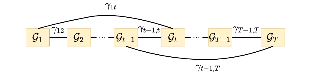
Formally, we define a temporal graph $\mathcal{G}_{N}=\{\mathcal{V}_{N},\mathcal{E}_{N}\}$, where $\mathcal{V}_{N}$ is the node set containing graphs of all time slots and $\mathcal{E}_{N}$ is the edge set containing connections between these graphs. In this paper, we suppose that there are $T$ nodes and $s$ edges in $\mathcal{G}_{N}$, i.e., $\left|\mathcal{V}_{N}\right|=T$ and $\left|\mathcal{E}_{N}\right|=s$. Time-varying graph learning using temporal graph is formulated as

where $\gamma_{ij}$ is the relative weights between the $i$-th and $j$-th time slots. Parameter $\eta$ is used to scale the weight of edge objectives relative to node objectives. Note that, (6) will boil down to (5) if we build $\mathcal{G}_{N}$ as a chain with equal weights.

We should mention that the design of $\mathcal{G}_{N}$, which is obtained by our prior knowledge of temporal relations, is critical for the learning performance. Better knowledge of temporal relations in real world does help improve the performance. The main contribution of temporal graph $\mathcal{G}_{N}$ is providing a more flexible structure to describe temporal relations fusing our prior knowledge. In the worst case, when we have no structured temporal priors, our framework can still boil down to model (5) but provides a more efficient algorithm introduced in the next section.

The algorithm for solving (5) attempts to learn $\mathcal{G}_{1},...,\mathcal{G}_{T}$ in a centralized fashion, resulting in increasing complexity as $T$. We hence develop a novel distributed algorithm based on ADMM framework [12, 13, 14] to solve (6). The algorithm is able to learn graphs of different time slots in parallel, showing its efficiency when $T$ is large. For an edge $(i,j)\in\mathcal{E}_{N}$, we first introduce a consensus variable of $\mathbf{w}_{i}$, denoted as $\mathbf{z}_{ij}$. In fact, $\mathbf{z}_{ij}$ represents the connection starting from $i$ to $j$. For the same edge, $\mathbf{z}_{ji}$ is the consensus variable of $\mathbf{w}_{j}$. With consensus variables, (6) is equivalent to the following problem

where $\mathcal{N}(i)$ denotes the set of all the nodes that are connected with node $i$ in $\mathcal{G}_{N}$. We define a matrix $\mathbf{W}\in\mathbb{R}^{p\times T}\triangleq[\mathbf{w}_{1},...,\mathbf{w}_{T}]$ containing all primal variables. In addition, matrices of consensus variables $\mathbf{Z}\in\mathbb{R}^{p\times 2s}$ and dual variables $\mathbf{U}\in\mathbb{R}^{p\times 2s}$ are also defined. For the $n$-th edge $(i,j)$ in temporal graph $\mathcal{G}_{N}$, $n=1,\ldots,s$, the corresponding consensus variable vectors $\mathbf{z}_{ij},\mathbf{z}_{ji}$ are the $(2n-1)$-th and $2n$-th columns of $\mathbf{Z}$, respectively. This also holds true for matrix $\mathbf{U}$. The scaled form of augmented Lagrangian of (7) is obtained as

where $\rho>0$ is an ADMM penalty parameter [14]. Following ADMM framework, we alternately update $\mathbf{W},\mathbf{U}$ and $\mathbf{Z}$.

1) Update $\mathbf{W}$: For $\mathbf{W}=[\mathbf{w}_{1},\ldots,\mathbf{w}_{T}]$, the update of $\left(\mathbf{w}^{k+1}_{t},1\leq t\leq T\right)$ is as follows

Obviously, we can update each $\mathbf{w}^{k+1}_{t}$ separately,

If we let $\bm{\theta}_{t}^{k}\triangleq\frac{1}{m}\sum_{j\in\mathcal{N}(t)}\left(\mathbf{z}_{tj}^{k}-\mathbf{u}_{tj}^{k}\right)$, where $m=|\mathcal{N}(t)|$, (10) can be reformulated as

In this paper, we use projected gradient descent (PGD) algorithm [16] to solve problem (11). The gradient of the objective function of (11) is as follows

where $.(-1)$ is an elementwise reciprocal operator. We set $\mathbf{y}^{0}=\mathbf{w}_{t}^{k}$ and iteratively update $\mathbf{y}^{r}$ using

until it converges to $\mathbf{y}^{*}$ with a certain precision, where $(\cdot)_{+}\triangleq\text{max}(\cdot,0)$, $r$ is the number of iterations of PGD algorithm and $\epsilon$ the step size. After obtaining the solution $\mathbf{y}^{*}$ of (11), we set $\mathbf{w}_{t}^{k+1}=\mathbf{y}^{*}$. Note that all $\mathbf{w}_{t}$ can be updated in parallel.

2) Update $\mathbf{Z}$: For each edge $(i,j)\in\mathcal{E}_{N}$, we can update the corresponding column vectors $\mathbf{z}_{ij},\mathbf{z}_{ji}$ of $\mathbf{Z}$ as follows

It is difficult to solve (14) due to that $\mathbf{z}_{ij}$ and $\mathbf{z}_{ji}$ are coupled with each other in $\left\lVert\mathbf{z}_{ij}-\mathbf{z}_{ji}\right\rVert_{1}$. Inspired by the method proposed in [17], we define a function $\tilde{\psi}$

with which (14) can be solved by

where $\mathrm{prox}_{\frac{\eta\gamma_{ij}}{\rho}\tilde{\psi}}(\cdot)$ is the proximal operator of function $\tilde{\psi}$ [18]. However, we have no knowledge of the closed form of the operator $\mathrm{prox}_{\frac{\eta\gamma_{ij}}{\rho}\tilde{\psi}}(\cdot)$. Hence a property of proximal operators mentioned in [17] might be introduced here.

In our problem, $h_{1}=\tilde{\psi},h_{2}=\ell_{1}$ norm, $\mathbf{G}=[-\mathbf{I}\,\,\,\mathbf{I}]$, $\mathbf{H}$ is zero matrix and $\lambda=\frac{1}{2}$. According to Property 1, the following update can be easily reached for (16),

Now each column of $\mathbf{Z}$ can be updated in parallel.

In summary, our algorithm can be implemented in a distributed fashion since the columns of $\mathbf{W},\mathbf{Z}$ and $\mathbf{U}$ can all be updated in parallel. The global convergence is also guaranteed by ADMM framework since (6) is a convex problem. Furthermore, the stopping criterion is that the primal and dual residuals are both below a given tolerance. More details can be referred in [14].

In this paper, we propose a general time-varying graph learning framework, under which temporal graph is employed to describe temporal structures. A distributed algorithm using ADMM framework is developed to solve the induced optimization problem. Experimental results show that our framework outperforms the state-of-art methods when facing complicated temporal structures.

References

- [1] G. Mateos, S. Segarra, A. G. Marques, and A. Ribeiro, “Connecting the dots: Identifying network structure via graph signal processing,” IEEE Signal Process. Mag., vol. 36, no. 3, pp.16–43, 2019.
- [2] V. Kalofolias, “How to learn a graph from smooth signals,” in Artif. Intel. and Stat. (AISTATS), 2016, pp. 920–929.
- [3] X. Dong, D. Thanou, P. Frossard, and P. Vandergheynst, “Learning laplacian matrix in smooth graph signal representations,” IEEE Trans. Signal Process., vol. 64, no. 23, pp. 6160–6173, 2016.
- [4] X. Dong, D. Thanou, M. Rabbat, and P. Frossard, “Learning graphs from data: A signal representation perspective,” IEEE Signal Process. Mag., vol. 36, no. 3, pp. 44–63, 2019.
- [5] Z. Wu, S. Pan, F. Chen, G. Long, C. Zhang, and S. Philip, “A comprehensive survey on graph neural networks,” IEEE Trans. Neural Netw Learn Syst., vol.32, no. 1, pp. 4–24, 2020.
- [6] J. Friedman, T. Hastie, and R. Tibshirani, “Sparse inverse covariance estimation with the graphicallasso,” Biostatistics, vol. 9, no. 3, pp. 432–441, 2008.
- [7] M. Yuan and Y. Lin, “Model selection and estimation in the gaussian graphical model,” Biometrika, vol. 94,no. 1, pp. 19–35, 2007.
- [8] A. Ortega, P. Frossard, and J. Kovačević, J. Moura and P. Vandergheynst, “Graph signal processing: Overview, challenges, and applications,” Proc. IEEE, vol. 106, no. 5, pp. 808–828, 2018.
- [9] V. Kalofolias, A. Loukas, D. Thanou, and P. Frossard, “Learning time varying graphs,” in IEEE Intl. Conf. Acoust., Speech and Signal Process. (ICASSP), 2017, pp. 2826–2830.
- [10] K. Yamada, Y. Tanaka, and A. Ortega, “Time-varying graph learning with constraints on graph temporal variation,” arXiv preprint arXiv:2001.03346 [eess.SP], 2020.
- [11] D. Thanou, X. Dong, D. Kressner, and P. Frossard, “Learning heat diffusion graphs,” IEEE Trans. Signal Inf. Proc. Netw., vol. 3, no. 3, pp. 484–499, 2017.
- [12] J. Nocedal and S. Wright, Numerical optimization, Springer Science & Business Media, 2006.
- [13] S. Boyd and L. Vandenberghe, Convex optimization, Cambridge university press, 2004.
- [14] S. Boyd, N. Parikh, and E. Chu, Distributed optimization and statistical learning via the alternating direction method of multipliers, Now Publishers Inc, 2011.
- [15] N. Komodakis and J. Pesquet, “Playing with duality: An overview of recent primal dual approaches for solving large-scale optimization problems,” IEEE Signal Process. Mag., vol. 32, no.6, pp. 31–54, 2015.
- [16] P. Calamai and J. More “Projected gradient methods for linearly constrained problems,” Math Program., vol. 39, no. 1, pp. 93–116, 1987.
- [17] D. Hallac, Y. Park, S. Boyd, and J. Leskovec, “Network inference via the time-varying Graphical Lasso,” in Proc. of the 23rd ACM SIGKDD International Conference on Knowledge Discovery and Data Mining, 2017, pp. 205–213.
- [18] N. Parikh and S. Boyd, “Proximal algorithms,” Foundations and Trends in optimization, vol. 1, no. 3, p. 127–239, 2014.
- [19] D. Powers, “Evaluation: from precision, recalland f-measure to roc, informedness, markedness andcorrelation,” arXiv preprint arXiv:2010.16061, 2020.
- [20] D. Hallac, J. Leskovec, and S. Boyd, “Network lasso: Clustering and optimization in large graphs,” in Proc. of the 21th ACM SIGKDD International Conference on Knowledge Discovery and Data Mining, 2015, pp. 387–396.