Kernel learning for sound field estimation
with $L_{1}$ and $L_{2}$ regularizations

Estimating and interpolating an acoustic field from discrete measurements of microphones are fundamental problems in acoustic signal processing. Such estimations can be applied to the visualization of acoustic fields [1], interpolation of room impulse responses [2, 3], identification of sound sources [4, 5], capturing sound fields for spatial audio [6, 7, 8], and spatial active noise control [9, 10], among others. We focus on the sound field estimation problem in a source-free region.

A typical strategy of sound field estimation is to decompose the measurements into spatial Fourier basis functions [11], such as plane waves [7] and spherical harmonics [12, 13]. However, the empirical setting of the truncation order and expansion center for the basis expansion is necessary. Sparsity-based approaches using the same basis functions have also been widely investigated [14, 15] to increase the spatial resolution. The main drawback of this method is that the inference operator of expansion coefficients becomes nonlinear. Thus, the estimation is basically performed by iterative processing.

The infinite-dimensional analysis of a sound field is proposed in [16], which corresponds to the kernel ridge regression when estimating a pressure field with pressure microphones [17]. This method does not require the empirical setting of truncation order and expansion center. Furthermore, the estimation is performed by a linear operation. In [18, 19], the kernel function using prior information on source directions is proposed. The estimation accuracy can be higher than that of the method without prior source direction [20, 17] by using the directionally weighted kernel.

The kernel function with directional weighting includes two parameters to be set, which are derived from the parameters of the von Mises–Fisher distribution [21]. One is the prior source directions and the other represents the spread of the weighting. In [18, 19], these parameters were empirically determined; however, source directions are not necessarily available in practical situations. Moreover, the optimal setting of the spread parameter is not a trivial task.

We propose a method to optimize the parameters of the directional kernel function from microphone measurements. We simplify the problem by discretizing the parameters and representing the kernel function as a weighted sum of sub-kernels. As a result, an optimization problem similar to the multiple kernel learning [22, 23] is derived. We investigate two types of regularizations for the weighting parameter to derive an algorithm for solving this problem. Although the kernel function is optimized by iterative processing, the estimation process is still a linear operation. We performed numerical simulations in a three-dimensional (3D) space to evaluate our proposed method.

Suppose a region of interest $\Omega\subseteq\mathbb{R}^{3}$ is a simply connected open subset of $\mathbb{R}^{3}$. The pressure field at the position $\bm{r}\in\Omega$ and angular frequency $\omega\in\mathbb{R}$ is denoted as $u(\bm{r},\omega)$ (i.e., $u:\Omega\times\mathbb{R}\rightarrow\mathbb{C}$). When $\Omega$ does not include any sources, $u$ satisfies the homogeneous Helmholtz equation as

where $\Delta$ denotes the Laplace operator and $k:=\omega/c$ is the wavenumber with the sound velocity $c$. We assume that the pressure field is measured by $M$ omnidirectional microphones arbitrarily placed inside $\Omega$. The position and observed signal of the $m$th microphone are denoted as $\bm{r}_{m}\in\Omega$ and $s_{m}(\omega)\in\mathbb{C}$, respectively, ($m\in\{1,\ldots,M\}$). Hereafter, $\omega$ is omitted for notational simplicity.

Our objective is to estimate $u(\bm{r})$ for $\bm{r}\in\Omega$ from the microphone measurements $\{s_{m}\}_{m=1}^{M}$ (see Fig. 1). This sound field estimation problem is formulated as follows:

where $\mathscr{H}$ is some function space for which we seek a solution, and $\|\cdot\|_{\mathscr{H}}$ is a norm on $\mathscr{H}$.

When $\mathscr{H}$ is a function space called a reproducing kernel Hilbert space (RKHS), (2) corresponds to kernel ridge regression [24]. We assume that RKHS $\mathscr{H}$ is defined with the inner product $\langle\cdot,\cdot\rangle_{\mathscr{H}}$ and positive-definite kernel $\kappa:\mathscr{H}\times\mathscr{H}\rightarrow\mathbb{C}$. On the basis of the representer theorem [25], its solution is represented as

where $\alpha_{m}\in\mathbb{C}$. Thus, (2) is transformed to the optimization problem for $\alpha_{m}$ and its solution is obtained as

where $\bm{\alpha}=[\alpha_{1},\ldots,\alpha_{M}]^{\mathsf{T}}$, $\bm{s}=[s_{1},\ldots,s_{M}]^{\mathsf{T}}$, and $\bm{K}$ is the Gram matrix defined as

An appropriate kernel function $\kappa$ associated with $\mathscr{H}$ and $\langle\cdot,\cdot\rangle_{\mathscr{H}}$ should be defined to obtain an appropriate estimate of $u(\bm{r})$.

We generalize the weighting function by a convex combination of (10) as

where $\gamma_{d}$ ($d\in\{1,\ldots,D\}$) is the weighting coefficient in $\mathbb{R}_{\geq 0}$, i.e., non-negative real constant. The parameters $\bm{\eta}$ and $\beta$ are discretized into $D_{\bm{\eta}}$ values of $\bm{\eta}_{d}$ and $D_{\beta}$ values of $\beta_{d}$ (i.e., $D=D_{\bm{\eta}}D_{\beta}$). Then, the kernel function is represented as the weighted sum of the sub-kernels as

where the sub-kernel $\kappa_{d}$ is given by (12) with $\bm{\eta}_{d}$ and $\beta_{d}$. Thus, problem (13) is transformed into the problem of determining $\gamma_{d}$ as well as $u$. This problem is known as multiple kernel learning [22, 23] in the context of machine learning. We also denote the vector of $\gamma_{d}$ as $\bm{\gamma}=[\gamma_{1},\ldots,\gamma_{D}]^{\mathsf{T}}\in\mathbb{R}_{\geq 0}^{D}$.

To jointly optimize $\bm{\gamma}$ and $u$, some constraint should be imposed on $\bm{\gamma}$ because excessively large $\bm{\gamma}$ can lead to a small cost function value. We investigate two types of regularization for $\bm{\gamma}$: $L_{1}$ and $L_{2}$.

We conducted numerical experiments in a 3D free field to evaluate the proposed method. For comparison, the method with the fixed kernel function without prior information of source directions [17] is used. This kernel function corresponds to (15) for $\beta=0$, i.e., uniform directional weighting $w(\bm{x})=1$, which becomes $\kappa(\bm{r}_{1},\bm{r}_{2})=j_{0}(k\|\bm{r}_{1}-\bm{r}_{2}\|)$.

The target region $\Omega$ was a sphere of radius $0.40~\mathrm{m}$, and the coordinate origin was set at the center of $\Omega$. Omnidirectional microphones were arranged on two layers of spherical surfaces, whose radii were $0.40~\mathrm{m}$ and $0.45~\mathrm{m}$, to avoid the non-uniqueness problem [11, 6]. The number of microphones was 25 for each layer, so the total number $M$ was 50. The microphones were arranged on each layer by using the spherical $t$-design [29]. Two point sources were placed at $(2.5,0.0,0.0)~\mathrm{m}$ and $(0.0,2.5,1.0)~\mathrm{m}$, and their amplitudes were both $20$. White Gaussian noise was added to the observation signals so that the signal-to-noise ratio (SNR) becomes $20~\mathrm{dB}$. The speed of sound was set to $340~\mathrm{m/s}$.

In the proposed method, the kernel functions $\kappa_{d}$ were obtained by discretizing $\bm{\eta}$ and $\beta$ into $10$ values each, i.e., $D_{\bm{\eta}}=10$ and $D_{\beta}=10$. The arrival directions $\bm{\eta}_{d}$ were set by regularly dividing the azimuth angle $[-\pi,\pi)$. The parameters $\beta_{d}$ were set from $0.0$ to $9.0$ at intervals of $1.0$.

As an evaluation measure, we define the following normalized mean squared error (NMSE):

where $u_{\mathrm{true}}$ and $u_{\mathrm{est}}$ respectively denote the true and estimated pressures, and $\{\bm{r}_{\mathrm{eval}}^{(i)}\}_{i\in I}$ denotes evaluation positions obtained by discretizing $\Omega$ every $0.05~\mathrm{m}$.

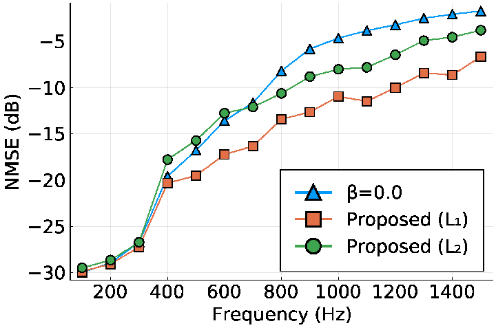
Fig. 2 shows the relationship between frequency and NMSE. The NMSEs of the two proposed methods were lower than that of the method using $\beta=0$. In particular, $L_{1}$ regularization performed better than $L_{2}$ regularization at all the frequencies. This result indicates that the sparsity constraint on $\bm{\gamma}$ was effective in this setting. On the other hand, the computational time of $L_{2}$ regularization was almost $10^{-2}$ times that of $L_{1}$ regularization for estimating $\bm{\gamma}$. As an example, the estimated pressure and normalized error distributions on the $x$-$y$-plane at $900~\mathrm{Hz}$ are shown in Figs. 4 and 4, respectively. In this case, 57% of $\gamma_{d}$ became $0$ in the $L_{1}$ regularization.

We proposed a kernel-interpolation-based sound field estimation method with learning kernels. The parameters for directional weighting in the kernel functions have been empirically determined on the basis of prior information on source directions; however, such information is not necessarily available in practical situations. To optimize these parameters on the basis of the observation values, we formulated the optimization problem by discretizing the parameters and representing the kernel function as the weighted sum of sub-kernels. Two types of regularization, $L_{1}$ and $L_{2}$, for the weights were investigated. Although the algorithms for solving these optimization problems are iterative processing, the estimation operation is linear and can be implemented using a finite response filter. The proposed method outperformed the method without the kernel learning in the numerical experiments.

This work was supported by JST PRESTO Grant Number JPMJPR18J4.

References

- [1] J. D. Maynard, E. G. Williams, and Y. Lee, “Nearfield acoustic holography: I. Theory of generalized holography and the development of NAH,” J. Acoust. Soc. Amer., vol. 78, no. 4, pp. 1395–1413, 1985.
- [2] R. Mignot, L. Daudet, and F. Ollivier, “Room reverberation reconstruction: Interpolation of the early part using compressed sensing,” IEEE Trans. Audio, Speech, Lang. Process., vol. 21, no. 11, pp. 2301–2312, 2013.
- [3] J. G. C. Ribeiro, N. Ueno, S. Koyama, and H. Saruwatari, “Kernel interpolation of acoustic transfer function between regions considering reciprocity,” in Proc. IEEE Sensor Array Multichannel Signal Process. Workshop (SAM), Jun. 2020.
- [4] M. Park and B. Rafaely, “Sound-field analysis by plane-wave decomposition using spherical microphone array,” J. Acoust. Soc. Amer., vol. 118, no. 5, pp. 3094–3103, 2005.
- [5] H. Teutsch and W. Kellermann, “Acoustic source detection and localization based on wavefield decomposition using circular microphone arrays,” J. Acoust. Soc. Amer., vol. 120, no. 5, pp. 2724–2736, 2006.
- [6] M. A. Poletti, “Three-dimensional surround sound systems based on spherical harmonics,” J. Audio Eng. Soc., vol. 53, no. 11, pp. 1004–1025, 2005.
- [7] S. Koyama, K. Furuya, Y. Hiwasaki, and Y. Haneda, “Analytical approach to wave field reconstruction filtering in spatio-temporal frequency domain,” IEEE Trans. Audio, Speech, Lang. Process., vol. 21, no. 4, pp. 685–696, 2013.
- [8] N. Iijima, S. Koyama, and H. Saruwatari, “Binaural rendering from distributed microphone signals considering loudspeaker distance in measurements,” in Proc. IEEE Int. Workshop Multimedia Signal Process. (MMSP), Tampere, Sep. 2020.
- [9] J. Zhang, T. D. Abhayapala, W. Zhang, P. N. Samarasinghe, and S. Jiang, “Active noise control over space: A wave domain approach,” IEEE/ACM Trans. Audio, Speech, Lang. Process., vol. 26, no. 4, pp. 774–786, 2018.
- [10] Y. Maeno, Y. Mitsufuji, P. N. Samarasinghe, N. Murata, and T. D. Abhayapala, “Spherical-harmonic-domain feedforward active noise control using sparse decomposition of reference signals from distributed sensor arrays,” IEEE/ACM Trans. Audio, Speech, Lang. Process., vol. 28, pp. 656–670, 2020.
- [11] E. Williams, Fourier Acoustics: Sound Radiation and Nearfield Acoustic Holography. London, UK: Academic Press, 1999.
- [12] A. Laborie, R. Bruno, and S. Montoya, “A new comprehensive approach of surround sound recording,” in Proc. 114th AES Conv., Amsterdam, 2003.
- [13] P. Samarasinghe, T. Abhayapala, and M. Poletti, “Wavefield analysis over large areas using distributed higher order microphones,” IEEE/ACM Trans. Audio, Speech, Lang. Process., vol. 22, no. 3, pp. 647–658, 2014.
- [14] A. Wabnitz, N. Epain, A. McEwan, and C. Jin, “Upscaling ambisonic sound scenes using compressed sensing techniques,” in Proc. IEEE Int. Workshop Appl. Signal Process. Audio Acoust. (WASPAA), New Paltz, 2011, pp. 1–4.
- [15] S. Koyama and L. Daudet, “Sparse representation of a spatial sound field in a reverberant environment,” IEEE J. Sel. Topics Signal Process., vol. 13, no. 1, pp. 172–184, 2019.
- [16] N. Ueno, S. Koyama, and H. Saruwatari, “Sound field recording using distributed microphones based on harmonic analysis of infinite order,” IEEE Signal Process. Lett., vol. 25, no. 1, pp. 135–139, 2018.
- [17] ——, “Kernel ridge regression with constraint of helmholtz equation for sound field interpolation,” in Proc. Int. Workshop Acoust. Signal Enhancement (IWAENC), Tokyo, Sep. 2018, pp. 436–440.
- [18] H. Ito, S. Koyama, N. Ueno, and H. Saruwatari, “Spatial active noise control based on kernel interpolation with directional weighting,” in Proc. IEEE Int. Conf. Acoust., Speech, Signal Process. (ICASSP), May 2020, pp. 8399–8403.
- [19] N. Ueno, S. Koyama, and H. Saruwatari, “Directionally weighted wave field estimation exploiting prior information on source direction,” IEEE Trans. Signal Process., 2021, (in press).
- [20] H. Ito, S. Koyama, N. Ueno, and H. Saruwatari, “Feedforward spatial active noise control based on kernel interpolation of sound field,” in Proc. IEEE Int. Conf. Acoust., Speech, Signal Process. (ICASSP), Brighton, May 2019, pp. 511–515.
- [21] K. V. Mardia and P. E. Jupp, Directional Statistics. Chichester: John Wiley & Sons, 2009, vol. 494.
- [22] M. Gönen and E. Alpaydın, “Multiple kernel learning algorithms,” J. Mach. Learn. Res., vol. 12, pp. 2211–2268, 2011.
- [23] S. Sonnenburg, G. Rätsch, C. Schäfer, and B. Schölkopf, “Large scale multiple kernel learning,” J. Mach. Learn. Res., vol. 7, pp. 1531–1565, 2006.
- [24] K. P. Murphy, Machine Learning: A Probabilistic Perspective. Cambridge: MIT Press, 2012.
- [25] F. Dinuzzo and B. Schölkopf, “The representer theorem for Hilbert spaces: a necessary and sufficient condition,” in Proc. Adv. Neural Inform. Process. Systems (NeurIPS), vol. 25, 2012.
- [26] F. Guevara Vasquez and C. Mauck, “Approximation by Herglotz wave functions,” SIAM J. Appl. Math., vol. 78, no. 3, pp. 1283–1299, 2018.
- [27] A. Rakotomamonjy, F. Bach, S. Canu, and Y. Grandvalet, “Simplemkl,” J. Mach. Learn. Res., vol. 9, pp. 2491–2521, 2008.
- [28] C. Cortes, M. Mohri, and A. Rostamizadeh, “L2 regularization for learning kernels,” in Proc. Conf. Uncertainty in Artificial Intelligence (UAI), Arlington, 2009, p. 109â116.
- [29] X. Chen and R. S. Womersley, “Existence of solutions to systems of underdetermined equations and spherical designs,” SIAM J. Numer. Anal., vol. 44, no. 6, pp. 2326–2341, 2006.