Deep Reinforcement Learning for Optimizing RIS-Assisted HD-FD Wireless Systems

Alice Faisal, Ibrahim Al-Nahhal, Octavia A. Dobre, and Telex M. N. Ngatched Thanks: A. Faisal, I. Al-Nahhal, O. A. Dobre, and T. M. N. Ngatched are with the Faculty of Engineering and Applied Science, Memorial University, St. John’s, NL, Canada, (e-mail: afaisal, ioalnahhal, odobre@mun.ca; tngatched@grenfell.mun.ca).

Abstract

This letter investigates the reconfigurable intelligent surface (RIS)-assisted multiple-input single-output (MISO) wireless system, where both half-duplex (HD) and full-duplex (FD) operating modes are considered together, for the first time in the literature. The goal is to maximize the rate by optimizing the RIS phase shifts. A novel deep reinforcement learning (DRL) algorithm is proposed to solve the formulated non-convex optimization problem. The complexity analysis and Monte Carlo simulations illustrate that the proposed DRL algorithm significantly improves the rate compared to the non-optimized scenario in both HD and FD operating modes using a single parameter setting. Besides, it significantly reduces the computational complexity of the downlink HD MISO system and improves the achievable rate with a reduced number of steps per episode compared to the conventional DRL algorithm.

Index Terms:

Reconfigurable intelligent surface (RIS), half-duplex full-duplex (HD-FD), deep reinforcement learning (DRL).

I Introduction

Reconfigurable intelligent surfaces (RIS) have emerged as a promising paradigm to fulfill the need of a smart and programmable wireless environment, and meet the demands of future wireless networks [1, 2]. RIS consists of a two-dimensional array of low-cost passive electromagnetic (EM) elements [3]. By overcoming the random nature of EM wave propagation, RIS enables controlling different characteristics of radio waves, such as scattering, reflection, and refraction. Consequently, it effectively enhances the signal quality and boosts the wireless spectral efficiency by realizing a controllable environment [4].

RIS-assisted multiple-input multiple-output systems have recently drawn significant attention as a cost-effective solution to enhance the wireless transmission in both half-duplex (HD) and full-duplex (FD) operating modes [5, 6, 7, 8, 9, 10]. In the HD mode, systems require additional resources to receive and forward signals, which results in a decreased spectral efficiency. In contrast, the FD mode has the potential to significantly increase the throughput of wireless systems as it enables simultaneous transmission and reception of signals in the same frequency band. However, this comes at the cost of increased interference and implementation complexity. To this end, some researchers are considering HD-FD transmission schemes that combine the advantages of both HD and FD modes [11]. In [5] and [6], RIS-HD systems are optimized to minimize the total transmit power. In [7], a joint optimization problem is considered to maximize the achievable rate of an RIS-HD system. In [8] and [9], the sum-rate and spectral efficiency of an RIS-FD system is maximized, respectively. In [10], the weighted minimum rate is maximized for a multi-user RIS-FD system. Most of these works decoupled the optimization variables using alternating optimization algorithms, which exhibit both loss of optimality and high computational complexity.

Deep learning has emerged as a powerful approach to optimize the RIS phase shifts by tackling the practical implementation problems of the optimization techniques [12, 13]. In particular, deep reinforcement learning (DRL) is a potential candidate to optimize the RIS phase shifts without the need for offline training with a labeled dataset. A few works have considered DRL approaches to optimize RIS-HD systems [14, 15, 16]. The authors in [14] proposed an optimization-driven deep deterministic policy gradient (DDPG) to minimize the access point’s transmit power. The sum-rate maximization problem of a multi-user RIS-HD system was addressed in [15] using a DRL algorithm. Furthermore, a conventional DRL algorithm is introduced in [16] to maximize the received signal-to-noise ratio of the downlink RIS-HD multiple-input single-output (MISO) system. To the best of the authors’ knowledge, utilizing DRL for RIS-FD systems has not yet been discussed in the literature.

In this letter, a novel DRL algorithm is proposed to optimize the phase shifts of an RIS-assisted HD-FD MISO system. The contributions are summarized as follows:

•

The proposed DRL algorithm achieves promising results in the HD and FD operating modes without the need of additional parameters tuning.
•

It provides a significant improvement in the rate compared to the non-optimized RIS phase shifts in the HD and FD operating modes.
•

It significantly reduces the computational complexity, while providing a considerable rate improvement with a reduced number of required steps for each episode, compared to the conventional DRL in [16] for the HD mode.
•

The complexity analysis and Monte Carlo simulations support the findings.

The remainder of this letter is organized as follows: Section II presents the system model and problem formulation for the RIS-assisted HD-FD MISO system. The proposed DRL algorithm is introduced in Section III, and its computational complexity is analyzed in Section IV. Simulation results and conclusions are presented in Sections V and VI, respectively.

II System Model and Problem Formulation

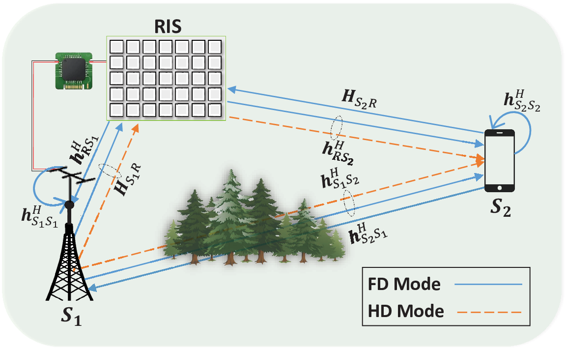
Consider an RIS-assisted HD-FD MISO system as illustrated in Fig. 1, where $S_{1}$ and $S_{2}$ represent the base station (BS) and user equipment (UE), respectively. Both the BS and UE are equipped with $M$ transmit antennas and one receive antenna. The UE sometimes operates in a HD mode, where it only receives information from the BS (i.e., downlink HD mode), while other times the UE and BS transmit and receive information simultaneously in the same frequency band (i.e., FD mode). Henceforth, $\Omega$ denotes the operating mode, where $\Omega\in\{\text{HD},\text{FD}\}$ . The RIS is composed of $N$ programmable reflecting elements, which assists the communication between $S_{1}$ and $S_{2}$ by optimizing the RIS phase shifts through an RIS controller. Given $\bar{i}=3-i$ $\forall\hskip 1.99997pti=1,2$ , let $\mathbf{H}_{{S_{\bar{i}}R}}\in\mathbb{C}^{N\times M}$ , $\mathbf{h}^{H}_{RS_{i}}\in\mathbb{C}^{1\times N}$ , and $\mathbf{h}^{H}_{{S_{\bar{i}}S_{i}}}\in\mathbb{C}^{1\times M}$ denote the channel coefficients of the $S_{\bar{i}}$ -RIS, RIS- $S_{i}$ , and $S_{\bar{i}}$ - $S_{i}$ links, respectively. The self-interference (SI) channels, which are involved in the FD mode at the BS and UE are denoted by $\mathbf{h}^{H}_{S_{i}S_{i}}\in\mathbb{C}^{1\times M}$ .

At the receiver-side, the signal is received from the direct and reflected links of the BS and RIS, respectively. Thus, the noisy received signals of the downlink HD and FD operating modes are respectively expressed as

y_{i}^{\Omega}=\Bigl(\underbrace{\mathbf{h}_{RS_{i}}^{H}\bm{\Theta}\mathbf{H}_{S_{\bar{i}}R}}_{\text{{Reflected signal}}}\hskip 5.69054pt+\hskip-2.84526pt\underbrace{\mathbf{h}_{{S_{\bar{i}}S_{i}}}^{H}}_{\text{Direct signal}}\hskip-5.69054pt\Bigr)\mathbf{w}_{\bar{i}}x_{\bar{i}}+n,\hskip 1.00006pti=2,\hskip 1.00006pt\Omega=\text{HD},

(1)

and

y_{i}^{\Omega}=\Bigl(\underbrace{\mathbf{h}_{RS_{i}}^{H}\bm{\Theta}\mathbf{H}_{S_{\bar{i}}R}}_{\text{Reflected signal}}\hskip 0.0pt+\hskip-8.53581pt\underbrace{\mathbf{h}_{{S_{\bar{i}}S_{i}}}^{H}}_{\text{\hskip 2.84526ptDirect signal}}\hskip-8.53581pt\Bigr)\mathbf{w}_{\bar{i}}x_{\bar{i}}\hskip 1.00006pt+\hskip 1.00006pt\underbrace{\mathbf{h}_{{S_{i}S_{i}}}^{H}\mathbf{w}_{i}x_{i}}_{\text{Residual SI}}+\hskip 1.00006ptn,\\ \hskip 1.00006pti=1,2,\Omega=\text{FD},

(2)

where $n\sim\mathcal{CN}(0,\sigma^{2})$ denotes the additive white complex Gaussian noise with zero-mean and variance $\sigma^{2}$ . The diagonal matrix $\bm{\Theta}=\text{diag}\bigl(e^{j\varphi_{1}},\cdots,e^{j\varphi_{n}},\cdots,e^{j\varphi_{N}}\bigr)\in\mathbb{C}^{N\times N}$ represents the phase shifts of the RIS, where $\varphi_{n}\in[-\pi,\pi)$ is the phase shift introduced by the $n$ -th reflecting element. The source node, $S_{i}$ , employs an active beamforming $\mathbf{w}_{i}\in\mathbb{C}^{M\times 1}$ to transmit the information signal, $x_{i}$ , with $\mathbb{E}\{|x_{i}|^{2}\}=1$ , where $\mathbb{E}\{\cdot\}$ denotes the expectation operation. The third term in (2) represents the SI introduced by the FD mode operation.

The achievable rate and sum-rate of the downlink HD and FD operating modes, measured in bit per second per Hertz (bps/Hz), are respectively given as

Refer to caption — Fig. 1: RIS-assisted HD-FD MISO system.

\mathcal{R}^{\Omega}=\text{log}_{2}\left(1+\frac{\left|\left(\mathbf{h}_{RS_{i}}^{H}\bm{\Theta}\mathbf{H}_{S_{\bar{i}}R}+\mathbf{h}_{{S_{\bar{i}}S_{i}}}^{H}\right)\mathbf{w}_{\bar{i}}\right|^{2}}{\sigma^{2}}\right),\hskip 1.00006pti=2,\hskip 1.00006pt\Omega=\text{HD},

(3)

and

\mathcal{R}^{\Omega}=\sum_{i=1}^{2}\text{log}_{2}\left(1+\frac{\left|\left(\mathbf{h}^{H}_{RS_{{i}}}\bm{\Theta}\mathbf{H}_{S_{\bar{i}}R}+\mathbf{h}^{H}_{S_{\bar{i}}S_{i}}\right)\mathbf{w}_{\bar{i}}\right|^{2}}{|\mathbf{h}^{H}_{S_{i}S_{i}}\mathbf{w}_{i}|^{2}+\sigma^{2}}\right),\hskip 1.00006pt\Omega=\text{FD}.

(4)

Here, the goal is to maximize the rate of the RIS-assisted HD-FD MISO system by optimizing the RIS phase shifts. Thus, the resulting optimization problem can be expressed as


(P1)	$\displaystyle\underset{\displaystyle\bm{\varphi}}{\mathrm{max}}\quad\mathcal{R}^{\Omega},\hskip 2.84526pt\Omega\in\{\text{HD},\text{FD}\}$		(5a)
	$\displaystyle\mathmakebox[\widthof{$\underset{\displaystyle\phantom{\bm{\varphi}}}{\mathrm{max}}$}][c]{\mathmakebox[\widthof{$\mathrm{max}$}][l]{\mathrm{\kern 1.00006pts.t.}}}\quad$	$\displaystyle{-\pi\leq\varphi_{n}\leq\pi,\hskip 1.99997ptn=1,\cdots,N.}$	(5b)

It is worth noting that the conventional DRL algorithm in [16] has been proposed to solve the non-convex problem (P1) only when $\Omega$ = HD, and suffers from high computational complexity. Moreover, the DRL for the FD operating mode has not yet been investigated in the literature.

III Proposed DRL Algorithm

This section proposes a novel DRL algorithm to solve (P1) for the RIS-assisted HD-FD MISO system. To deal with (P1), the RIS phase shifts are optimized using the proposed DRL algorithm. Then, for a given optimized $\bm{\Theta}$ , the transmit beamformers, $\mathbf{w}_{\bar{i}}$ , are optimized using a closed and semi-closed form solutions for the HD and FD operating modes, respectively. The optimization problem is solved in an iterative fashion until the optimized $\bm{\Theta}$ and $\mathbf{w}_{\bar{i}}$ converge.

III-A Beamforming Design for a Given $\mathbf{\Theta}$

The optimal beamforming vector for the HD operating mode is calculated using the maximum ratio transmission approach, whereas a semi-closed optimal solution of the FD beamforming vectors is given in [8]. Consequently, for a given optimized $\bm{\Theta}$ , the optimal beamforming vectors of the HD and FD modes, $\mathbf{w}_{\bar{i}}$ , are respectively given as

\mathbf{w}_{\bar{i}}^{\dagger}=\sqrt{P_{\text{max}}}\frac{\left(\mathbf{h}_{RS_{i}}^{H}\bm{\Theta}\mathbf{H}_{S_{\bar{i}}R}+\mathbf{h}_{{S_{\bar{i}}S_{i}}}^{H}\right)^{H}}{\left|\left|\left(\mathbf{h}_{RS_{i}}^{H}\bm{\Theta}\mathbf{H}_{S_{\bar{i}}R}+\mathbf{h}_{{S_{\bar{i}}S_{i}}}^{H}\right)\right|\right|},\hskip 1.00006pti=2,\hskip 1.00006pt\Omega=\text{HD},

(6)

and

\mathbf{w}^{\dagger}_{\bar{i}}=(\delta\mathbf{h}_{S_{\bar{i}}S_{\bar{i}}}\mathbf{h}^{H}_{S_{\bar{i}}S_{\bar{i}}}+v^{\dagger}\mathbf{I})^{-1}\bm{\mathcal{B}},\hskip 1.00006pti=1,2,\hskip 1.00006pt\Omega=\text{FD},

(7)

where $P_{\text{max}}$ is the maximum transmitted power of $S_{\bar{i}}$ , $\mathbf{I}$ is the identity matrix, and $v^{\dagger}$ is the optimal dual Lagrangian variable associated with the power constraint that is found by performing a bisection search over the interval $\left[0,\sqrt{\bm{\mathcal{B}}^{T}\bm{\mathcal{B}}}/\sqrt{P_{\text{max}}}\right]$ . Here, $\bm{\mathcal{B}}$ and $\delta$ are given as

\bm{\mathcal{B}}\triangleq\frac{1}{\tilde{b}_{i}}\left(1+\frac{b_{{i}}}{|\mathbf{h}_{S_{\bar{i}}S_{\bar{i}}}^{H}\mathbf{\tilde{w}}_{\bar{i}}|^{2}+\sigma^{2}}\right)\mathbf{h}_{\bar{i}}\mathbf{h}^{H}_{\bar{i}}\mathbf{\tilde{w}}_{\bar{i}},

(8)

and

\delta\triangleq\frac{b_{{i}}\left(|\mathbf{h}^{H}_{\bar{i}}\mathbf{\tilde{w}}_{\bar{i}}|^{2}+\tilde{b}_{i}\right)}{\tilde{b}_{i}\left(|\mathbf{h}_{S_{\bar{i}}S_{\bar{i}}}^{H}\mathbf{\tilde{w}}_{\bar{i}}|^{2}+\sigma^{2}\right)^{2}},

(9)

where $b_{{i}}\triangleq|\mathbf{h}^{H}_{{i}}\mathbf{w}_{{i}}|^{2}$ , $\tilde{b}_{i}\triangleq|\mathbf{h}^{H}_{S_{i}S_{{i}}}\mathbf{w}_{i}|^{2}$ $+$ $\sigma^{2}$ , $\mathbf{h}_{\bar{i}}\triangleq\mathbf{H}^{H}_{S_{\bar{i}}R}\bm{\Theta}^{H}\mathbf{h}_{RS_{{i}}}+\mathbf{h}_{S_{\bar{i}}S_{{i}}}$ , and $\mathbf{\tilde{w}}_{\bar{i}}$ is a given feasible point.

III-B Phase Shift Design Based on the Proposed DRL Algorithm

III-B1 Problem Transformation

The RIS controller represents the DRL agent, while the RIS-assisted HD-FD MISO communication system represents the DRL environment. Thus, the state space, action space, and reward for the proposed DRL algorithm are defined as follows:

•

State space: The state space at time step $t$ , $s_{t}\in\mathbb{R}^{1\times(N+1)}$ , includes $\varphi_{n}\hskip 1.00006pt{\forall\hskip 1.99997ptn}=1,\cdots,N$ and the corresponding $\mathcal{R}^{\Omega}$ at time step $t-1$ , and is defined as

$s_{t}=\left[\mathcal{R}^{\Omega,(t-1)},\varphi^{(t-1)}_{1},\cdots,\varphi^{(t-1)}_{n},\cdots,\varphi^{(t-1)}_{N}\right].$ (10)
•

Action space: Since (P1) aims to optimize the RIS phase shifts, the action space at time step $t$ , $a_{t}\in\mathbb{R}^{1\times N}$ , is expressed as

$a_{t}=\left[\varphi^{(t)}_{1},\cdots,\varphi^{(t)}_{n},\cdots,\varphi^{(t)}_{N}\right].$ (11)
•

Reward: As the target of (P1) is to maximize $\mathcal{R}^{\Omega}$ , the reward is expressed as

$r_{t}=\mathcal{R}^{\Omega,(t)},\hskip 2.84526pt\Omega\in\{\text{HD},\text{FD}\}.$ (12)

At each time step $t$ , the agent receives the current state $s_{t}$ from the environment, takes an action $a_{t}$ based on a policy $\tilde{\pi}$ , and receives a scalar reward $r_{t}$ . Then, a new state $s_{t+1}$ is obtained. The return of a state is defined as the total discounted reward from time step $t$ onwards, and is given by $R_{t}=\sum_{k=t}^{\infty}\gamma^{k-t}r(s_{k},a_{k})$ , where $\gamma\in(0,1]$ is the DRL discount factor. The goal is to learn a policy that maximizes the expected cumulative discounted reward from the start state, as: $J(\tilde{\pi})=\mathbb{E}\left[R_{1}|\tilde{\pi}\right]$ . The DDPG, which combines the benefits of value-based and policy-based approaches [17], is used to learn the optimal policy for a continuous $a_{t}$ . In particular, the DDPG algorithm aims at maximizing the Q-value of $(s,a)$ pair by training a deep neural network (DNN), defined as

Q^{\tilde{\pi}_{\bm{\theta}}}(s,a)=\mathbb{E}_{\tilde{\pi}_{\bm{\theta}}}\biggl[R_{1}|s_{1}=s,a_{1}=a\biggr],

(13)

where $\bm{\theta}$ represents the DNN parameters, as well as finding the optimal policy by performing the gradient ascent of

\nabla_{\bm{\theta}}J(\tilde{\pi}_{\bm{\theta}})=\mathbb{E}_{\tilde{\pi}_{\bm{\theta}}}\left[Q^{\tilde{\pi}_{\bm{\theta}}}(s,a)\nabla_{\bm{\theta}}\text{log}\pi_{\bm{\theta}}(a|s)\right].

(14)

The DDPG algorithm is based on the actor-critic technique, which consists of two DNN models: actor and critic. The actor, $\mu(s_{t}|\bm{\theta}_{\mu})$ , represents the policy network that takes the state as an input for a given $\bm{\theta}_{\mu}$ and outputs $a_{t}=\mu(s_{t}|\bm{\theta}_{\mu})+\xi$ , where $\xi$ is a random process that is added to the actions for exploration. $\xi$ is modeled as complex Gaussian process with zero mean and variance 0.1. The critic, $Q(s_{t},a_{t}|\bm{\theta}_{q})$ , represents the network that evaluates the actions. It takes $s_{t}$ and $a_{t}$ as an input for a given $\bm{\theta}_{q}$ , and outputs the Q-value. The DDPG algorithm utilizes the concept of experience replay with memory $D$ to reduce the correlation of the training samples by randomly sampling minibatch transitions, $N_{B}$ . Moreover, target networks are introduced to stabilize the learning process. The target networks are generated by making a copy of the actor and critic evaluation NNs, $\mu^{\prime}(s_{t}|\bm{\theta}_{\mu^{\prime}})$ and $Q^{\prime}(s_{t},a_{t}|\bm{\theta}_{q^{\prime}})$ , and are used to calculate the corresponding target values, $y_{t}$ in (15). The actor and critic NN parameters, $\bm{\theta}_{\mu}$ and $\bm{\theta}_{q}$ , are updated using the stochastic gradient descent (SGD) from (16) and policy gradient from (17), respectively. Finally, the target NN parameters are updated using a soft update coefficient, $\tau$ , based on (18) and (19). After $T$ steps of each episode, the agent’s performance saturates and it outputs the optimized $\Theta$ . The structure of the proposed DRL algorithm is illustrated in Fig. 2 and summarized in Algorithm 1.

Algorithm 1 Proposed DRL algorithm.

\bm{\theta}_{\mu}

and

\bm{\theta}_{q}

with random weights,

D

\gamma

\tau

, and learning rate

\alpha

; Set:

\bm{\theta}_{\mu^{\prime}}\leftarrow\bm{\theta}_{\mu}

and

\bm{\theta}_{q^{\prime}}\leftarrow\bm{\theta}_{q}

;

2: repeat

Collect the channels of the

k

-th episode based on

\Omega

;

Randomly initialize

\varphi_{n}\hskip 1.99997pt{\forall\hskip 1.99997pt}n=1,\cdots,N

to obtain the initial state;

5: if

\Omega=\text{HD}

then

6: Calculate

\mathbf{w}_{\bar{i}}

using (6);

7: else

8: Calculate

\mathbf{w}_{\bar{i}}

using (7);

9: end if

10: Initialize

\xi\sim\mathcal{CN}(0,0.1)

;

11: repeat

12:

Obtain

a_{t}=\mu(s_{t}|\bm{\theta}_{\mu})+\xi

from the actor network and reshape it;

13: Repeat Lines #4-8;

14: Observe the new state,

s_{t+1}

, given

a_{t}

;

15:

Store (

s_{t},a_{t},r_{t},s_{t+1}

) in

D

;

16:

When

D

is full, sample a minibatch of

N_{B}

transitions randomly (

s_{j},a_{j},r_{j},s_{j+1}

) from

D

;

17: Compute the target value using target networks:

y_{j}=r_{j}+\gamma Q^{\prime}(s_{j+1},\mu^{\prime}(s_{j+1}|\bm{\theta}_{\mu^{\prime}})|\bm{\theta}_{q^{\prime}});

(15)

18:

Update the critic by minimizing the loss using SGD:

L=\frac{1}{N_{B}}\sum_{j}\left(y_{j}-Q(s_{j},a_{j}|\bm{\theta}_{q})\right)^{2};

(16)

19: Update the actor using the policy gradient:

\nabla_{\bm{\theta}_{\mu}}=\frac{1}{N_{B}}\sum_{j}\nabla_{a}Q(s,a|\bm{\theta}_{q})|_{s=s_{j},a=\mu(s_{j})}\nabla_{\bm{\theta}_{\mu}}\mu(s|\bm{\theta}_{\mu})|_{s_{j}};

(17)

20: Update the target NNs through soft update:

\bm{\theta}_{q^{\prime}}\longleftarrow\tau\bm{\theta}_{q}+(1-\tau)\bm{\theta}_{q^{\prime}},

(18)

\bm{\theta}_{\mu^{\prime}}\longleftarrow\tau\bm{\theta}_{\mu^{\prime}}+(1-\tau)\bm{\theta}_{\mu^{\prime}}.

(19)

21: until

t=T

;

22: until

k=K

;

23: Optimal action that corresponds to the optimal

\bm{\Theta}

III-B2 Proposed DNN Design

As can be seen from Fig. 2, the proposed DRL algorithm contains four NNs (i.e., two NNs for the actor and two NNs for the critic). A novel design is proposed for the four NNs, which consists of the input layer, two hidden layers and the output layer. The two hidden layers are a combination of one convolutional layer and one feed-forward (FF) layer with a flatten layer between them. The input layer of the actor and critic networks contains $N+1$ neurons (i.e., size of $s_{t}$ ) and $2N+1$ neurons (i.e., concatenation of $s_{t}$ and $a_{t}$ ), respectively. The output layer of the actor and critic networks contains $N$ neurons (i.e., size of $a_{t}$ ) and one neuron (i.e., scalar Q-value), respectively. The convolutional hidden layer for each of the actor and critic networks uses the ReLU activation function since it does not suffer from vanishing or exploding problems. In contrast, the FF hidden layer uses the softmax activation function to obtain probabilistic values for all inputs.

IV Complexity Analysis

The computational complexity of the conventional DRL algorithm in [16] and the proposed DRL algorithm for $\Omega=\text{HD}$ is derived in terms of the number of NN parameters $C_{\mathcal{P}}$ required to be stored, real additions $C_{\mathcal{A}}$ , and real multiplications $C_{\mathcal{M}}$ . The conventional DRL algorithm uses two hidden FF layers, and its computational complexity is given as

		$\displaystyle C_{\mathcal{P}}=\sum_{i=1}^{3}(\eta_{i}+1)\eta_{i+1},$		(20)
		$\displaystyle C_{\mathcal{M}}=\sum_{i=1}^{3}\eta_{i}\eta_{i+1},$		(21)
		$\displaystyle C_{\mathcal{A}}=\sum_{i=1}^{3}\eta_{i}\eta_{i+1}+\sum_{i=1}^{3}\eta_{i+1},$		(22)

where $\eta_{i}$ is the number of neurons of the $i$ -th layer. It is worth noting that, for simplicity, each activation function is considered to cost one real addition.

Based on the NNs design in Section III-B2, the complexity for the proposed DRL algorithm is given as

		$\displaystyle C_{\mathcal{P}}=(\eta_{F}\eta_{3}+F_{z}+1)F_{n}+(\eta_{4}+1)\eta_{3}+\eta_{4},$		(23)
		$\displaystyle C_{\mathcal{M}}=(F_{z}+\eta_{3})\eta_{F}F_{n}+\eta_{3}\eta_{4},$		(24)
		$\displaystyle C_{\mathcal{A}}=(F_{z}+\eta_{3}+1)\eta_{F}F_{n}+(\eta_{4}+1)\eta_{3}+\eta_{4},$		(25)

where $\eta_{F}=\lfloor\frac{\eta_{1}-{F_{z}}}{F_{s}}+1\rfloor$ , with $\lfloor\cdot\rfloor$ as the floor operation, $F_{z}$ is the filter size, $F_{n}$ is the number of filters, and $F_{s}$ is the stride. The complexity reduction of using the proposed DRL algorithm over the conventional one for $\Omega=\text{HD}$ is

\text{Reduction}=1-\frac{\left\{C^{\text{Actor}}_{\chi}+C^{\text{Critic}}_{\chi}\right\}_{\text{Proposed}}}{\left\{C^{\text{Actor}}_{\chi}+C^{\text{Critic}}_{\chi}\right\}_{\text{{Conventional}}}},\hskip 1.99997pt\chi\in\{\mathcal{P},\mathcal{A},\mathcal{M}\}.

(26)

V Simulation Results

This section evaluates the performance of the proposed DRL algorithm for the RIS-assisted HD-FD MISO system. The simulation setup is shown in Fig. 3, where the considered parameters are $d_{v}=2\,\mathrm{m}$ and $d_{1}=50\,\mathrm{m}$ . The distances of the BS-RIS and UE-RIS links are calculated as $d_{2}=\sqrt{d^{2}_{0}+d^{2}_{v}}$ m and $d_{3}=\sqrt{(d_{1}-d_{0})^{2}+d^{2}_{v}}$ m, respectively. The path loss (PL) at distance $d_{j}$ , $\forall j\in\{1,2,3\}$ is modeled as $\text{PL}=PL_{0}-10\zeta\text{log}_{10}\left(\frac{d_{j}}{{D_{r}}}\right)$ [16], where $PL_{0}$ is the PL at a reference distance ${D_{r}}$ and $\zeta$ is the PL exponent, in which $PL_{0}={-30\,\mathrm{dB}}$ and ${D_{r}}=1\,\mathrm{m}$ . As in [16], the BS-UE channels are modeled as Rayleigh fading (assuming a blocking element between $S_{1}$ and $S_{2}$ ), while the rest of the channels are Rician with a factor of $10$ . The PL exponents of the BS-UE, BS-RIS, and UE-RIS channels are set to $\zeta_{\text{BU}}=3$ and $\zeta_{\text{BR}}=\zeta_{\text{UR}}=2$ , respectively. The PL of the SI channels for the FD mode is $-95\,\mathrm{dB}$ . The total transmit power is $P=5\,\mathrm{dBm}$ , while the noise power is $\sigma^{2}=-80\,\mathrm{dBm}$ . The antenna gain at the BS and UE is $0\,\mathrm{dBi}$ , while the RIS gain is $5\,\mathrm{dBi}$ . The penetration loss in the BS-UE and RIS-UE links is $10\,\mathrm{dB}$ .

The parameters of the proposed DRL algorithm are summarized in Fig. 3. Furthermore, the design of the NNs is explained in Section III-B2, and its parameters are provided in Fig. 3. The Adam optimizer is used to update the parameters of the NNs. To assess the performance of the proposed algorithm, it is compared with the non-optimized scenario, referred to as random phase shifts. The conventional DRL algorithm in [16] with $T=1000$ is also included to show the superiority of the proposed DRL algorithm in the HD mode. It is worth noting that the current form of the conventional DRL algorithm can not be used to optimize the RIS phase shifts in the FD mode.

Figure. 4 studies the impact of the RIS location on the system performance. It is shown that the proposed DRL algorithm significantly improves the rate for both operating modes, compared to the random phase shifts and without-RIS scenarios, especially when the RIS is located closer to either the BS or the UE. On the other hand, the random phase shifts scenario does not improve the rate when the RIS is located relatively far from both BS and UE, compared to the scenario without-RIS. Consequently, a proper optimization for the RIS phase shifts is needed to achieve a satisfactory performance. For the rest of the letter, it is considered that $d_{0}=1\,\mathrm{m}$ .

Figure. 5 illustrates the effect of increasing $N$ on the system performance. As can be observed, $R^{\Omega}$ increases as $N$ increases for all algorithms. The proposed DRL algorithm provides an improvement of 4.6 bps/Hz and 8.5 bps/Hz in the achievable rate and sum-rate of the HD and FD modes, respectively, compared to the random phase shifts scenario at $N=40$ . It is worth noting that the gain gap increases as $N$ increases for the proposed DRL algorithm.

In the HD operating mode, the proposed DRL algorithm improves the achievable rate performance by 1.4 bps/Hz and 0.6 bps/Hz at $N=20$ and $N=40$ , respectively, when compared to [16], as depicted in Fig. 5. Moreover, as shown in Fig. 6(a), the proposed DRL algorithm in the HD mode (with $T=800$ steps) significantly reduces the computational complexity of each NN in the range of 94% to 86% for the practical case of $N=20$ to $60$ , respectively, compared to conventional DRL in [16] (with $T=1000$ steps). Although the complexity reduction seems to decrease as $N$ increases, it saturates at 63% for a certain large value of $N$ , as seen from the asymptotic complexity bound in Fig. 6(b).

Finally, the proposed DRL algorithm provides a significant improvement in the rate for both operating modes, compared with the random phase shifts scenario. Besides, with a 20% reduction in the number of required steps when compared with the conventional DRL algorithm, the proposed DRL algorithm guarantees a faster convergence and improves the rate with lower computational complexity for each of the four NNs.

VI Conclusion

This letter considered DRL for the rate maximization problem of the RIS-assisted HD-FD MISO system, for the first time in the literature. With a single parameter setting, the proposed DRL algorithm optimized the RIS phase shifts for both HD and FD operating modes. A novel DNN structure was proposed to learn the optimal policy of the proposed DRL algorithm. Compared to the non-optimized scenario, the proposed DRL algorithm significantly improved the rate for the HD and FD operating modes, respectively. Compared to the conventional DRL algorithm in HD mode, the proposed DRL algorithm saved 20% of the required steps per episode and achieved up to 1.4 bps/Hz rate improvement with up to 94% reduction in the computational complexity. Future works can consider extending the proposed DRL algorithm to optimize the multi-user scenario.

References

[1] I. Al-Nahhal et al., “Reconfigurable intelligent surface-assisted uplink sparse code multiple access,” IEEE Commun. Lett., vol. 25, no. 6, pp. 2058–2062, Feb. 2021.
[2] L. Bariah et al., “A prospective look: Key enabling technologies, applications and open research topics in 6G networks,” IEEE Access, vol. 8, pp. 174792–174820, Aug. 2020.
[3] E. Basar et al., “Wireless communications through reconfigurable intelligent surfaces,” IEEE Access, vol. 7, pp. 116753–116773, Aug. 2019.
[4] R. Alghamdi et al., “Intelligent surfaces for 6G wireless networks: A survey of optimization and performance analysis techniques,” IEEE Access, vol. 8, pp. 202795–202818, Oct. 2020.
[5] Q. Wu and R. Zhang, “Beamforming optimization for wireless network aided by intelligent reflecting surface with discrete phase shifts,” IEEE Trans. Commun., vol. 68, no. 3, pp. 1838–1851, Dec. 2020.
[6] G. Zhou et al., “Robust beamforming design for intelligent reflecting surface aided MISO communication systems,” IEEE Wireless Commun. Lett., vol. 9, no. 10, pp. 1658–1662, Jun. 2020.
[7] N. S. Perović et al., “Achievable rate optimization for MIMO systems with reconfigurable intelligent surfaces,” IEEE Trans. Wireless Commun., vol. 20, no. 6, pp. 3865–3882, Feb. 2021.
[8] H. Shen et al., “Beamformig design with fast convergence for IRS-aided full-duplex communication,” IEEE Commun. Lett., vol. 24, no. 12, pp. 2849–2853, Aug. 2020.
[9] J. Zhao et al., “Energy efficient full-duplex communication systems with reconfigurable intelligent surface,” in Proc. IEEE Veh. Technol. Conf. (VTC Fall), Feb. 2020, pp. 1–5.
[10] Z. Peng et al., “Multiuser full-duplex two-way communications via intelligent reflecting surface,” IEEE Trans. Signal Process., vol. 69, pp. 837–851, Jan. 2021.
[11] M. Elhattab et al., “Reconfigurable intelligent surface enabled full-duplex/half-duplex cooperative non-orthogonal multiple access,” Jan. 2021. [Online]. Available: https://arxiv.org/abs/2101.01307
[12] A. Zappone et al., “Wireless networks design in the era of deep learning: Model-based, AI-based, or both?” IEEE Trans. Commun., vol. 67, no. 10, pp. 7331–7376, Jun. 2019.
[13] Y. Chen et al., “Reinforcement learning meets wireless networks: A layering perspective,” IEEE Internet Things J., vol. 8, no. 1, pp. 85–111, Jan. 2021.
[14] J. Lin et al., “Deep reinforcement learning for robust beamforming in IRS-assisted wireless communications,” in Proc. IEEE Global Commun. Conf. (GLOBECOM), Jan. 2020, pp. 1–6.
[15] C. Huang et al., “Reconfigurable intelligent surface assisted multiuser MISO systems exploiting deep reinforcement learning,” IEEE J. Sel. Areas Commun., vol. 38, no. 8, pp. 1839–1850, Jun. 2020.
[16] K. Feng et al., “Deep reinforcement learning based intelligent reflecting surface optimization for MISO communication systems,” IEEE Wireless Commun. Lett., vol. 9, no. 5, pp. 745–749, Jan. 2020.
[17] T. P. Lillicrap et al., “Continuous control with deep reinforcement learning,” in Proc. Int. Conf. Learn. Represent. (ICLR), May 2016, pp. 1–14.