Heavy Ball Neural Ordinary Differential Equations

Hedi XiaDepartment of MathematicsUniversity of California, Los AngelesVai Suliafu Scientific Computing and Imaging (SCI) InstituteUniversity of Utah, Salt Lake City, UT, USAHangjie JiDepartment of MathematicsUniversity of California, Los AngelesTan M. NguyenDepartment of MathematicsUniversity of California, Los AngelesAndrea L. BertozziDepartment of MathematicsUniversity of California, Los AngelesStanley J. OsherDepartment of MathematicsUniversity of California, Los AngelesBao Wang Department of MathematicsScientific Computing and Imaging (SCI) InstituteUniversity of Utah, Salt Lake City, UT, USA Thanks: Co-first author Thanks: Please correspond to: wangbaonj@gmail.com

Abstract

We propose heavy ball neural ordinary differential equations (HBNODEs), leveraging the continuous limit of the classical momentum accelerated gradient descent, to improve neural ODEs (NODEs) training and inference. HBNODEs have two properties that imply practical advantages over NODEs: (i) The adjoint state of an HBNODE also satisfies an HBNODE, accelerating both forward and backward ODE solvers, thus significantly reducing the number of function evaluations (NFEs) and improving the utility of the trained models. (ii) The spectrum of HBNODEs is well structured, enabling effective learning of long-term dependencies from complex sequential data. We verify the advantages of HBNODEs over NODEs on benchmark tasks, including image classification, learning complex dynamics, and sequential modeling. Our method requires remarkably fewer forward and backward NFEs, is more accurate, and learns long-term dependencies more effectively than the other ODE-based neural network models. Code is available at https://github.com/hedixia/HeavyBallNODE.

1 Introduction

Neural ordinary differential equations (NODEs) are a family of continuous-depth machine learning (ML) models whose forward and backward propagations rely on solving an ODE and its adjoint equation (Chen et al. 2018). NODEs model the dynamics of hidden features ${\bm{h}}(t)\in{\mathbb{R}}^{N}$ using an ODE, which is parametrized by a neural network $f({\bm{h}}(t),t,\theta)\in{\mathbb{R}}^{N}$ with learnable parameters $\theta$ , i.e.,

\frac{d{\bm{h}}(t)}{dt}=f({\bm{h}}(t),t,\theta).

(1)

Figure 1: Contrasting NODE, ANODE, SONODE, HBNODE, and GHBNODE for CIFAR10 classification in NFEs, training time, and test accuracy. (Tolerance:

10^{-5}

, see Sec. 5.2 for experimental details.)

Starting from the input ${\bm{h}}(t_{0})$ , NODEs obtain the output ${\bm{h}}(T)$ by solving (1) for $t_{0}\leq t\leq T$ with the initial value ${\bm{h}}(t_{0})$ , using a black-box numerical ODE solver. The number of function evaluations (NFEs) that the black-box ODE solver requires in a single forward pass is an analogue for the continuous-depth models (Chen et al. 2018) to the depth of networks in ResNets. The loss between NODE prediction ${\bm{h}}(T)$ and the ground truth is denoted by $\mathcal{L}({\bm{h}}(T))$ ; we update parameters $\theta$ using the following gradient (Pontryagin 2018)

\frac{d\mathcal{L}({\bm{h}}(T))}{d\theta}=\int_{t_{0}}^{T}{\bm{a}}(t)\frac{\partial f({\bm{h}}(t),t,\theta)}{\partial\theta}dt,

(2)

where ${\bm{a}}(t):=\partial\mathcal{L}/\partial{\bm{h}}(t)$ is the adjoint state, which satisfies the adjoint equation

\frac{d{\bm{a}}(t)}{dt}=-{\bm{a}}(t)\frac{\partial f({\bm{h}}(t),t,\theta)}{\partial{\bm{h}}}.

(3)

NODEs are flexible in learning from irregularly-sampled sequential data and particularly suitable for learning complex dynamical systems (Chen et al. 2018; Rubanova et al. 2019; Zhang et al. 2019; Norcliffe et al. 2020; Du et al. 2020; Kidger et al. 2020), which can be trained by efficient algorithms (Quaglino et al. 2020; Daulbaev et al. 2020; Zhuang et al. 2021). NODE-based continuous generative models have computational advantages over the classical normalizing flows (Chen et al. 2018; Grathwohl et al. 2019; Yildiz et al. 2019; Finlay et al. 2020). NODEs have also been generalized to neural stochastic differential equations, stochastic processes, and graph NODEs (Jia and Benson 2019; Li et al. 2020; Poli et al. 2019; Tzen and Raginsky 2019; Huang et al. 2020; Norcliffe et al. 2021). The drawback of NODEs is also prominent. In many ML tasks, NODEs require very high NFEs in both training and inference, especially in high accuracy settings where a lower tolerance is needed. The NFEs increase rapidly with training; high NFEs reduce computational speed and accuracy of NODEs and can lead to blow-ups in the worst-case scenario (Grathwohl et al. 2019; Dupont et al. 2019; Massaroli et al. 2020; Norcliffe et al. 2020). As an illustration, we train NODEs for CIFAR10 classification using the same model and experimental settings as in (Dupont et al. 2019), except using a tolerance of $10^{-5}$ ; Fig. 1 shows both forward and backward NFEs and the training time of different ODE-based models; we see that NFEs and computational times increase very rapidly for NODE, ANODE (Dupont et al. 2019), and SONODE (Norcliffe et al. 2020). More results on the large NFE and degrading utility issues for different benchmark experiments are available in Sec. 5. Another issue is that NODEs often fail to effectively learn long-term dependencies in sequential data (Lechner and Hasani 2020), discussed in Sec. 4.

1.1 Contribution

We propose heavy ball neural ODEs (HBNODEs), leveraging the continuous limit of the classical momentum accelerated gradient descent, to improve NODE training and inference. At the core of HBNODE is replacing the first-order ODE (1) with a heavy ball ODE (HBODE), i.e., a second-order ODE with an appropriate damping term. HBNODEs have two theoretical properties that imply practical advantages over NODEs:

•

The adjoint equation used for training a HBNODE is also a HBNODE (see Prop. 1 and Prop. 2), accelerating both forward and backward propagation, thus significantly reducing both forward and backward NFEs. The reduction in NFE using HBNODE over existing benchmark ODE-based models becomes more aggressive as the error tolerance of the ODE solvers decreases.
•

The spectrum of the HBODE is well-structured (see Prop. 4), alleviating the vanishing gradient issue in back-propagation and enabling the model to effectively learn long-term dependencies from sequential data.

To mitigate the potential blow-up problem in training HBNODEs, we further propose generalized HBNODEs (GHBNODEs) by integrating skip connections (He et al. 2016) and gating mechanisms (Hochreiter and Schmidhuber 1997) into the HBNODE. See Sec. 3 for details.

1.2 Organization

We organize the paper as follows: In Secs 2 and 3, we present our motivation, algorithm, and analysis of HBNODEs and GHBNODEs, respectively. We analyze the spectrum structure of the adjoint equation of HBNODEs/GHBNODEs in Sec. 4, which indicates that HBNODEs/GHBNODEs can learn long-term dependency effectively. We test the performance of HBNODEs and GHBNODEs on benchmark point cloud separation, image classification, learning dynamics, and sequential modeling in Sec. 5. We discuss more related work in Sec. 6, followed by concluding remarks. Technical proofs and more experimental details are provided in the appendix.

2 Heavy Ball Neural Ordinary Differential Equations

2.1 Heavy ball ordinary differential equation

Classical momentum method, a.k.a., the heavy ball method, has achieved remarkable success in accelerating gradient descent (Polyak 1964) and has significantly improved the training of deep neural networks (Sutskever et al. 2013). As the continuous limit of the classical momentum method, heavy ball ODE (HBODE) has been studied in various settings and has been used to analyze the acceleration phenomenon of the momentum methods. For the ease of reading and completeness, we derive the HBODE from the classical momentum method. Starting from initial points ${\bm{x}}^{0}$ and ${\bm{x}}^{1}$ , gradient descent with classical momentum searches a minimum of the function $F({\bm{x}})$ through the following iteration

{\bm{x}}^{k+1}={\bm{x}}^{k}-s\nabla F({\bm{x}}^{k})+\beta({\bm{x}}^{k}-{\bm{x}}^{k-1}),

(4)

where $s>0$ is the step size and $0\leq\beta<1$ is the momentum hyperparameter. For any fixed step size $s$ , let ${\bm{m}}^{k}:=({{\bm{x}}^{k+1}-{\bm{x}}^{k}})/{\sqrt{s}},$ and let $\beta:=1-\gamma\sqrt{s}$ , where $\gamma\geq 0$ is another hyperparameter. Then we can rewrite (4) as

{\bm{m}}^{k+1}=(1-\gamma\sqrt{s}){\bm{m}}^{k}-\sqrt{s}\nabla F({\bm{x}}^{k});\ {\bm{x}}^{k+1}={\bm{x}}^{k}+\sqrt{s}{\bm{m}}^{k+1}.

(5)

Let $s\to 0$ in (5); we obtain the following system of first-order ODEs,

\frac{d{\bm{x}}(t)}{dt}={\bm{m}}(t);\ \frac{d{\bm{m}}(t)}{dt}=-\gamma{\bm{m}}(t)-\nabla F({\bm{x}}(t)).

(6)

This can be further rewritten as a second-order heavy ball ODE (HBODE), which also models a damped oscillator,

\frac{d^{2}{\bm{x}}(t)}{dt^{2}}+\gamma\frac{d{\bm{x}}(t)}{dt}=-\nabla F({\bm{x}}(t)).

(7)

Figure 2: Comparing the trajectory of ODE and HBODE when

F({\bm{x}})

is the Rosenbrock (left) and Beale (right) functions.

We compare the dynamics of HBODE (7) and the following ODE limit of the gradient descent (GD)

\frac{d{\bm{x}}}{dt}=-\nabla F({\bm{x}}).

(8)

In particular, we solve the ODEs (7) and (8) with $F({\bm{x}})$ defined as a Rosenbrock (Rosenbrock 1960) or Beale (Gonçalves 1971) function (see Appendix E.6 for experimental details). Fig. 2 shows that with the same numerical ODE solver, HBODE converges to the stationary point (marked by stars) faster than (8). The fact that HBODE can accelerate the dynamics of the ODE for a gradient system motivates us to propose HBNODE to accelerate forward propagation of NODE.

2.2 Heavy ball neural ordinary differential equations

Similar to NODE, we parameterize $-\nabla F$ in (7) using a neural network $f({\bm{h}}(t),t,\theta)$ , resulting in the following HBNODE with initial position ${\bm{h}}(t_{0})$ and momentum ${\bm{m}}(t_{0}):=d{\bm{h}}/dt(t_{0})$ ,

\frac{d^{2}{\bm{h}}(t)}{dt^{2}}+\gamma\frac{d{\bm{h}}(t)}{dt}=f({\bm{h}}(t),t,\theta),

(9)

where $\gamma\geq 0$ is the damping parameter, which can be set as a tunable or a learnable hyperparmater with positivity constraint. In the trainable case, we use $\gamma=\epsilon\cdot\text{sigmoid}(\omega)$ for a trainable $\omega\in\mathbb{R}$ and a fixed tunable upper bound $\epsilon$ (we set $\epsilon=1$ below). According to (6), HBNODE (9) is equivalent to

\frac{d{\bm{h}}(t)}{dt}={\bm{m}}(t);\quad\frac{d{\bm{m}}(t)}{dt}=-\gamma{\bm{m}}(t)+f({\bm{h}}(t),t,\theta).

(10)

Equation (9) (or equivalently, the system (10)) defines the forward ODE for the HBNODE, and we can use either the first-order (Prop. 2) or the second-order (Prop. 1) adjoint sensitivity method to update the parameter $\theta$ (Norcliffe et al. 2020).

Proposition 1 (Adjoint equation for HBNODE).

The adjoint state ${\bm{a}}(t):=\partial\mathcal{L}/\partial{\bm{h}}(t)$ for the HBNODE (9) satisfies the following HBODE with the same damping parameter $\gamma$ as that in (9),

\frac{d^{2}{\bm{a}}(t)}{dt^{2}}-\gamma\frac{d{\bm{a}}(t)}{dt}={\bm{a}}(t)\frac{\partial f}{\partial{\bm{h}}}({\bm{h}}(t),t,\theta).

(11)

Remark 1.

Note that we solve the adjoint equation (11) from time $t=T$ to $t=t_{0}$ in the backward propagation. By letting $\tau=T-t$ and ${\bm{b}}(\tau)={\bm{a}}(T-\tau)$ , we can rewrite (11) as follows,

\frac{d^{2}{\bm{b}}(\tau)}{d\tau^{2}}+\gamma\frac{d{\bm{b}}(\tau)}{d\tau}={\bm{b}}(\tau)\frac{\partial f}{\partial{\bm{h}}}({\bm{h}}(T-\tau),T-\tau,\theta).

(12)

Therefore, the adjoint of the HBNODE is also a HBNODE and they have the same damping parameter.

We can also employ (10) and its adjoint for the forward and backward propagations, respectively.

Proposition 2 (Adjoint equations for the first-order HBNODE system).

The adjoint states ${\bm{a}}_{\bm{h}}(t)$ $:=\partial\mathcal{L}/\partial{\bm{h}}(t)$ and ${\bm{a}}_{\bm{m}}(t):=\partial\mathcal{L}/\partial{\bm{m}}(t)$ for the first-order HBNODE system (10) satisfy

\frac{d{\bm{a}}_{\bm{h}}(t)}{dt}=-{\bm{a}}_{\bm{m}}(t)\frac{\partial f}{\partial{\bm{h}}}({\bm{h}}(t),t,\theta);\quad\frac{d{\bm{a}}_{\bm{m}}(t)}{dt}=-{\bm{a}}_{\bm{h}}(t)+\gamma{\bm{a}}_{\bm{m}}(t).

(13)

Remark 2.

Let $\tilde{{\bm{a}}}_{\bm{m}}(t)=d{\bm{a}}_{\bm{m}}(t)/dt$ , then ${\bm{a}}_{\bm{m}}(t)$ and $\tilde{{\bm{a}}}_{\bm{m}}(t)$ satisfies the following first-order heavy ball ODE system

\frac{d{\bm{a}}_{\bm{m}}(t)}{dt}=\tilde{{\bm{a}}}_{\bm{m}}(t);\quad\frac{d\tilde{{\bm{a}}}_{\bm{m}}(t)}{dt}={\bm{a}}_{\bm{m}}(t)\frac{\partial f}{\partial{\bm{h}}}({\bm{h}}(t),t,\theta)+\gamma\tilde{{\bm{a}}}_{\bm{m}}(t).

(14)

Note that we solve this system backward in time in back-propagation. Moreover, we have ${\bm{a}}_{{\bm{h}}}(t)=\gamma{\bm{a}}_{\bm{m}}(t)-\tilde{{\bm{a}}}_{\bm{m}}(t)$ .

Similar to (Norcliffe et al. 2020), we use the coupled first-order HBNODE system (10) and its adjoint first-order HBNODE system (13) for practical implementation, since the entangled representation permits faster computation (Norcliffe et al. 2020) of the gradients of the coupled ODE systems.

3 Generalized Heavy Ball Neural Ordinary Differential Equations

Figure 3: Contrasting

{\bm{h}}(t)

for different models.

{\bm{h}}(t)

in ANODE, SONODE, and HBNODE grows much faster than that in NODE. GHBNODE controls the growth of

{\bm{h}}(t)

effectively when

t

is large.

In this section, we propose a generalized version of HBNODE (GHBNODE), see (15), to mitigate the potential blow-up issue in training ODE-based models. In our experiments, we observe that ${\bm{h}}(t)$ of ANODEs (Dupont et al. 2019), SONODEs (Norcliffe et al. 2020), and HBNODEs (10) usually grows much faster than that of NODEs. The fast growth of ${\bm{h}}(t)$ can lead to finite-time blow up. As an illustration, we compare the performance of NODE, ANODE, SONODE, HBNODE, and GHBNODE on the Silverbox task as in (Norcliffe et al. 2020). The goal of the task is to learn the voltage of an electronic circuit that resembles a Duffing oscillator, where the input voltage $V_{1}(t)$ is used to predict the output $V_{2}(t)$ . Similar to the setting in (Norcliffe et al. 2020), we first augment ANODE by 1 dimension with 0-augmentation and augment SONODE, HBNODE, and GHBNODE with a dense network. We use a simple dense layer to parameterize $f$ for all five models, with an extra input term for $V_{1}(t)$ ¹¹ 1 Here, we exclude an ${\bm{h}}^{3}$ term that appeared in the original Duffing oscillator model because including it would result in finite-time explosion.. For both HBNODE and GHBNODE, we set the damping parameter $\gamma$ to be ${\rm sigmoid}(-3)$ . For GHBNODE (15) below, we set $\sigma(\cdot)$ to be the hardtanh function with bound $[-5,5]$ and $\xi=\ln(2)$ . The detailed architecture can be found in Appendix E. As shown in Fig. 3, compared to the vanilla NODE, the $\ell_{2}$ norm of ${\bm{h}}(t)$ grows much faster when a higher order NODE is used, which leads to blow-up during training. Similar issues arise in the time series experiments (see Sec. 5.4), where SONODE blows up during long term integration in time, and HBNODE suffers from the same issue with some initialization.

To alleviate the problem above, we propose the following generalized HBNODE

	$\displaystyle\frac{d{\bm{h}}(t)}{dt}$	$\displaystyle=\sigma({\bm{m}}(t)),$		(15)
	$\displaystyle\frac{d{\bm{m}}(t)}{dt}$	$\displaystyle=-\gamma{\bm{m}}(t)+f({\bm{h}}(t),t,\theta)-\xi{\bm{h}}(t),$		(15)

where $\sigma(\cdot)$ is a nonlinear activation, which is set as $\tanh$ in our experiments. The positive hyperparameters $\gamma,\xi>0$ are tunable or learnable. In the trainable case, we let $\gamma=\epsilon\cdot\text{sigmoid}(\omega)$ as in HBNODE, and $\xi=\text{softplus}(\chi)$ to ensure that $\gamma,\xi\geq 0$ . Here, we integrate two main ideas into the design of GHBNODE: (i) We incorporate the gating mechanism used in LSTM (Hochreiter and Schmidhuber 1997) and GRU (Cho et al. 2014), which can suppress the aggregation of ${\bm{m}}(t)$ ; (ii) Following the idea of skip connection (He et al. 2016), we add the term $\xi{\bm{h}}(t)$ into the governing equation of ${\bm{m}}(t)$ , which benefits training and generalization of GHBNODEs. Fig. 3 shows that GHBNODE can indeed control the growth of ${\bm{h}}(t)$ effectively.

Proposition 3 (Adjoint equations for GHBNODEs).

The adjoint states ${\bm{a}}_{\bm{h}}(t):=\partial\mathcal{L}/\partial{\bm{h}}(t)$ , ${\bm{a}}_{\bm{m}}(t):=\partial\mathcal{L}/\partial{\bm{m}}(t)$ for the GHBNODE (15) satisfy the following first-order ODE system

\frac{\partial{\bm{a}}_{\bm{h}}(t)}{\partial t}=-{\bm{a}}_{\bm{m}}(t)\Big(\frac{\partial f}{\partial{\bm{h}}}({\bm{h}}(t),t,\theta)-\xi{\bm{I}}\Big),\quad\frac{\partial{\bm{a}}_{\bm{m}}(t)}{\partial t}=-{\bm{a}}_{\bm{h}}(t)\sigma^{\prime}({\bm{m}}(t))+\gamma{\bm{a}}_{\bm{m}}(t).

(16)

Though the adjoint state of the GHBNODE (16) does not satisfy the exact heavy ball ODE, based on our empirical study, it also significantly reduces the backward NFEs.

4 Learning long-term dependencies – Vanishing gradient

It is known that the vanishing and exploding gradients are two bottlenecks for training recurrent neural networks (RNNs) with long-term dependencies (Bengio et al. 1994; Pascanu et al. 2013) (see Appendix C for a brief review on the exploding and vanishing gradient issues in training RNNs). The exploding gradients issue can be effectively resolved via gradient clipping, training loss regularization, etc (Pascanu et al. 2013; Erichson et al. 2021). Thus in practice the vanishing gradient is the major issue for learning long-term dependencies (Pascanu et al. 2013). As the continuous analogue of RNN, NODEs as well as their hybrid ODE-RNN models, may also suffer from vanishing in the adjoint state ${\bm{a}}(t):=\partial\mathcal{L}/\partial{\bm{h}}(t)$ (Lechner and Hasani 2020). When the vanishing gradient issue happens, ${\bm{a}}(t)$ goes to ${\bf 0}$ quickly as $T-t$ increases, then $d\mathcal{L}/d\theta$ in (2) will be independent of these ${\bm{a}}(t)$ . We have the following expressions for the adjoint states of the NODE and HBNODE (see Appendix C for detailed derivation):

•

For NODE, we have

\frac{\partial\mathcal{L}}{\partial{\bm{h}}_{t}}=\frac{\partial\mathcal{L}}{\partial{\bm{h}}_{T}}\frac{\partial{\bm{h}}_{T}}{\partial{\bm{h}}_{t}}=\frac{\partial\mathcal{L}}{\partial{\bm{h}}_{T}}\exp\Big\{-\int_{T}^{t}\frac{\partial f}{\partial{\bm{h}}}({\bm{h}}(s),s,\theta)ds\Big\}.

(17)

•

For GHBNODE²² 2 HBNODE can be seen as a special GHBNODE with $\xi=0$ and $\sigma$ be the identity map., from (13) we can derive

{\small\begin{bmatrix}\frac{\partial\mathcal{L}}{\partial{\bm{h}}_{t}}&\hskip-7.22743pt\frac{\partial\mathcal{L}}{\partial{\bm{m}}_{t}}\end{bmatrix}=\begin{bmatrix}\frac{\partial\mathcal{L}}{\partial{\bm{h}}_{T}}&\hskip-7.22743pt\frac{\partial\mathcal{L}}{\partial{\bm{m}}_{T}}\end{bmatrix}\begin{bmatrix}\frac{\partial{\bm{h}}_{T}}{\partial{\bm{h}}_{t}}&\hskip-7.22743pt\frac{\partial{\bm{h}}_{T}}{\partial{\bm{m}}_{t}}\\ \frac{\partial{\bm{m}}_{T}}{\partial{\bm{h}}_{t}}&\hskip-7.22743pt\frac{\partial{\bm{m}}_{T}}{\partial{\bm{m}}_{t}}\\ \end{bmatrix}=\begin{bmatrix}\frac{\partial\mathcal{L}}{\partial{\bm{h}}_{T}}\ \frac{\partial\mathcal{L}}{\partial{\bm{m}}_{T}}\end{bmatrix}\exp\Big\{-\underbrace{\int_{T}^{t}\begin{bmatrix}{\bf 0}&\hskip-3.61371pt\frac{\partial\sigma}{\partial{\bm{m}}}\\ \big(\frac{\partial f}{\partial{\bm{h}}}-\xi{\bm{I}}\big)&\hskip-3.61371pt-\gamma{\bm{I}}\end{bmatrix}ds}_{:={\bm{M}}}\Big\}.}

(18)

Note that the matrix exponential is directly related to its eigenvalues. By Schur decomposition, there exists an orthogonal matrix ${\bm{Q}}$ and an upper triangular matrix ${\bm{U}}$ , where the diagonal entries of ${\bm{U}}$ are eigenvalues of ${\bm{Q}}$ ordered by their real parts, such that

-{\bm{M}}={\bm{Q}}{\bm{U}}{\bm{Q}}^{\top}\Longrightarrow\exp\{-{\bm{M}}\}={\bm{Q}}\exp\{{\bm{U}}\}{\bm{Q}}^{\top}.

(19)

Let ${\bm{v}}^{\top}:=\begin{bmatrix}\frac{\partial\mathcal{L}}{\partial{\bm{h}}_{T}}\ \frac{\partial\mathcal{L}}{\partial{\bm{m}}_{T}}\end{bmatrix}{\bm{Q}}$ , then (18) can be rewritten as

\begin{bmatrix}\frac{\partial\mathcal{L}}{\partial{\bm{h}}_{t}}\ \frac{\partial\mathcal{L}}{\partial{\bm{m}}_{t}}\end{bmatrix}=\begin{bmatrix}\frac{\partial\mathcal{L}}{\partial{\bm{h}}_{T}}\ \frac{\partial\mathcal{L}}{\partial{\bm{m}}_{T}}\end{bmatrix}\exp\{-{\bm{M}}\}=\begin{bmatrix}\frac{\partial\mathcal{L}}{\partial{\bm{h}}_{T}}\ \frac{\partial\mathcal{L}}{\partial{\bm{m}}_{T}}\end{bmatrix}{\bm{Q}}\exp\{{\bm{U}}\}{\bm{Q}}^{\top}={\bm{v}}^{\top}\exp\{{\bm{U}}\}{\bm{Q}}^{\top}.

(20)

By taking the $\ell_{2}$ norm in (20) and dividing both sides by $\left\lVert\begin{bmatrix}\frac{\partial\mathcal{L}}{\partial{\bm{h}}_{T}}\ \frac{\partial\mathcal{L}}{\partial{\bm{m}}_{T}}\end{bmatrix}\right\rVert_{2}$ , we arrive at

\frac{\left\lVert\begin{bmatrix}\frac{\partial\mathcal{L}}{\partial{\bm{h}}_{t}}\ \frac{\partial\mathcal{L}}{\partial{\bm{m}}_{t}}\end{bmatrix}\right\rVert_{2}}{\left\lVert\begin{bmatrix}\frac{\partial\mathcal{L}}{\partial{\bm{h}}_{T}}\ \frac{\partial\mathcal{L}}{\partial{\bm{m}}_{T}}\end{bmatrix}\right\rVert_{2}}=\frac{\left\lVert{\bm{v}}^{\top}\exp\{{\bm{U}}\}{\bm{Q}}^{\top}\right\rVert_{2}}{\left\lVert{\bm{v}}^{\top}{\bm{Q}}^{\top}\right\rVert_{2}}=\frac{\left\lVert{\bm{v}}^{\top}\exp\{{\bm{U}}\}\right\rVert_{2}}{\left\lVert{\bm{v}}\right\rVert_{2}}=\left\lVert{\bm{e}}^{\top}\exp\{{\bm{U}}\}\right\rVert_{2},

(21)

i.e., $\left\lVert\begin{bmatrix}\frac{\partial\mathcal{L}}{\partial{\bm{h}}_{t}}\ \frac{\partial\mathcal{L}}{\partial{\bm{m}}_{t}}\end{bmatrix}\right\rVert_{2}=\left\lVert{\bm{e}}^{\top}\exp\{{\bm{U}}\}\right\rVert_{2}\left\lVert\begin{bmatrix}\frac{\partial\mathcal{L}}{\partial{\bm{h}}_{T}}\ \frac{\partial\mathcal{L}}{\partial{\bm{m}}_{T}}\end{bmatrix}\right\rVert_{2}$ where ${\bm{e}}={{\bm{v}}}/{\left\lVert{\bm{v}}\right\rVert_{2}}$ .

Proposition 4.

The eigenvalues of $-{\bm{M}}$ can be paired so that the sum of each pair equals $(t-T)\gamma$ .

For a given constant $a>0$ , we can group the upper triangular matrix $\exp\{{\bm{U}}\}$ as follows

\exp\{{\bm{U}}\}:=\begin{bmatrix}\exp\{{\bm{U}}_{L}\}&{\bm{P}}\\ {\bf 0}&\exp\{{\bm{U}}_{V}\}\end{bmatrix},

(22)

where the diagonal of ${\bm{U}}_{L}$ ( ${\bm{U}}_{V}$ ) contains eigenvalues of $-{\bm{M}}$ that are no less (greater) than $(t-T)a$ . Then, we have $\|{\bm{e}}^{\top}\exp\{{\bm{U}}\}\|_{2}\geq\|{\bm{e}}_{L}^{\top}\exp\{{\bm{U}}_{L}\}\|_{2}$ where the vector ${\bm{e}}_{L}$ denotes the first $m$ columns of ${\bm{e}}$ with $m$ be the number of columns of ${\bm{U}}_{L}$ . By choosing $0\leq\gamma\leq 2a$ , for every pair of eigenvalues of $-{\bm{M}}$ there is at least one eigenvalue whose real part is no less than $(t-T)a$ . Therefore, $\exp\{{\bm{U}}_{L}\}$ decays at a rate at most $(t-T)a$ , and the dimension of ${\bm{U}}_{L}$ is at least $N\times N$ . We avoid exploding gradients by clipping the $\ell_{2}$ norm of the adjoint states similar to that used for training RNNs.

In contrast, all eigenvalues of the matrix $\int_{T}^{t}{\partial f}/{\partial{\bm{h}}}ds$ in (17) for NODE can be very positive or negative, resulting in exploding or vanishing gradients. As an illustration, we consider the benchmark Walker2D kinematic simulation task that requires learning long-term dependencies effectively (Lechner and Hasani 2020; Brockman et al. 2016). We train ODE-RNN (Rubanova et al. 2019) and (G)HBNODE-RNN on this benchmark dataset, and the detailed experimental settings are provided in Sec. 5.4. Figure 4 plots $\|\partial\mathcal{L}/\partial{\bm{h}}_{t}\|_{2}$ for ODE-RNN and $\|[\partial\mathcal{L}/\partial{\bm{h}}_{t}\ \partial\mathcal{L}/\partial{\bm{m}}_{t}]\|_{2}$ for (G)HBNODE-RNN, showing that the adjoint state of ODE-RNN vanishes quickly, while that of (G)HBNODE-RNN does not vanish even when the gap between $T$ and $t$ is very large.

Refer to caption — Figure 4: Plot of the the $\ell_{2}$ -norm of the adjoint states for ODE-RNN and (G)HBNODE-RNN back-propagated from the last time stamp. The adjoint state of ODE-RNN vanishes quickly when the gap between the final time $T$ and intermediate time $t$ becomes larger, while the adjoint states of (G)HBNODE-RNN decays much more slowly. This implies that (G)HBNODE-RNN is more effective in learning long-term dependency than ODE-RNN.

5 Experimental Results

In this section, we compare the performance of the proposed HBNODE and GHBNODE with existing ODE-based models, including NODE (Chen et al. 2018), ANODE (Dupont et al. 2019), and SONODE (Norcliffe et al. 2020) on the benchmark point cloud separation, image classification, learning dynamical systems, and kinematic simulation. For all the experiments, we use Adam (Kingma and Ba 2014) as the benchmark optimization solver (the learning rate and batch size for each experiment are listed in Table 1) and Dormand–Prince-45 as the numerical ODE solver. For HBNODE and GHBNODE, we set $\gamma={\rm sigmoid}(\theta)$ , where $\theta$ is a trainable weight initialized as $\theta=-3$ . The network architecture used to parameterize $f({\bm{h}}(t),t,\theta)$ for each experiment below are described in Appendix E. All experiments are conducted on a server with 2 NVIDIA Titan Xp GPUs.

Table 1: The batch size and learning rate for different datasets.

Dataset	Point Cloud	MNIST	CIFAR10	Plane Vibration	Walker2D
Batch Size	50	64	64	64	256
Learning Rate	0.01	0.001	0.001	0.0001	0.003

5.1 Point cloud separation

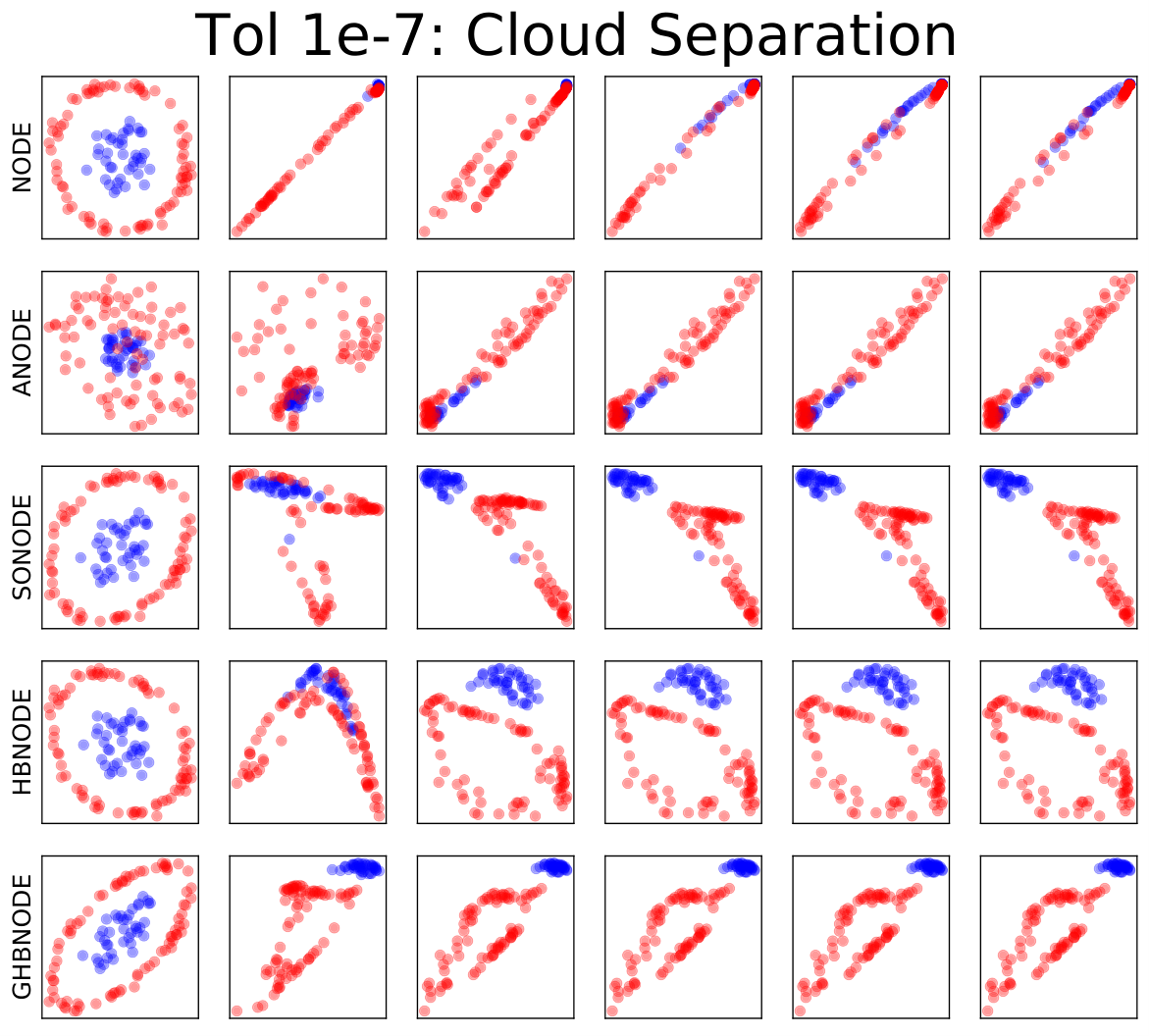
In this subsection, we consider the two-dimensional point cloud separation benchmark. A total of $120$ points are sampled, in which $40$ points are drawn uniformly from the circle $\|{\bm{r}}\|<0.5$ , and $80$ points are drawn uniformly from the annulus $0.85<\|{\bm{r}}\|<1.0$ . This experiment aims to learn effective features to classify these two point clouds. Following Dupont et al. 2019, we use a three-layer neural network to parameterize the right-hand side of each ODE-based model, integrate the ODE-based model from $t_{0}=0$ to $T=1$ , and pass the integration results to a dense layer to generate the classification results. We set the size of hidden layers so that the models have similar sizes, and the number of parameters of NODE, ANODE, SONODE, HBNODE, and GHBNODE are $525$ , $567$ , $528$ , $568$ , and $568$ , respectively. To avoid the effects of numerical error of the black-box ODE solver we set tolerance of ODE solver to be $10^{-7}$ . Figure 5 plots a randomly selected evolution of the point cloud separation for each model; we also compare the forward and backward NFEs and the training loss of these models (100 independent runs). HBNODE and GHBNODE improve training as the training loss consistently goes to zero over different runs, while ANODE and SONODE often get stuck at local minima, and NODE cannot separate the point cloud since it preserves the topology (Dupont et al. 2019).

5.2 Image classification

We compare the performance of HBNODE and GHBNODE with the existing ODE-based models on MNIST and CIFAR10 classification tasks using the same setting as in Dupont et al. 2019. We parameterize $f({\bm{h}}(t),t,\theta)$ using a 3-layer convolutional network for each ODE-based model, and the total number of parameters for each model is listed in Table 2. For a given input image of the size $c\times h\times w$ , we first augment the number of channel from $c$ to $c+p$ with the augmentation dimension $p$ dependent on each method³³ 3 We set $p=0,5,4,4,5/0,10,9,9,9$ on MNIST/CIFAR10 for NODE, ANODE, SONODE, HBNODE, and GHBNODE, respectively.. Moreover, for SONODE, HBNODE and GHBNODE, we further include velocity or momentum with the same shape as the augmented state.

Table 2: The number of parameters for each models for image classification.

Model	NODE	ANODE	SONODE	HBNODE	GHBNODE
#Params (MNIST)	85,315	85,462	86,179	85,931	85,235
#Params (CIFAR10)	173,611	172,452	171,635	172,916	172,916

Figure 6: Contrasting NODE (Chen et al. 2018), ANODE (Dupont et al. 2019), SONODE (Norcliffe et al. 2020), HBNODE, and GHBNODE for MNIST classification in NFE, training time, and test accuracy. (Tolerance:

10^{-5}

NFEs.

As shown in Figs. 1 and 6, the NFEs grow rapidly with training of the NODE, resulting in an increasingly complex model with reduced performance and the possibility of blow up. Input augmentation has been verified to effectively reduce the NFEs, as both ANODE and SONODE require fewer forward NFEs than NODE for the MNIST and CIFAR10 classification. However, input augmentation is less effective in controlling their backward NFEs. HBNODE and GHBNODE require much fewer NFEs than the existing benchmarks, especially for backward NFEs. In practice, reducing NFEs implies reducing both training and inference time, as shown in Figs. 1 and 6.

Accuracy.

We also compare the accuracy of different ODE-based models for MNIST and CIFAR10 classification. As shown in Figs. 1 and 6, HBNODE and GHBNODE have slightly better classification accuracy than the other three models; this resonates with the fact that less NFEs lead to simpler models which generalize better (Dupont et al. 2019; Norcliffe et al. 2020).

NFEs vs. tolerance.

We further study the NFEs for different ODE-based models under different tolerances of the ODE solver using the same approach as in Chen et al. 2018. Figure 7 depicts the forward and backward NFEs for different models under different tolerances. We see that (i) both forward and backward NFEs grow quickly when tolerance is decreased, and HBNODE and GHBNODE require much fewer NFEs than other models; (ii) under different tolerances, the backward NFEs of NODE, ANODE, and SONODE are much larger than the forward NFEs, and the difference becomes larger when the tolerance decreases. In contrast, the forward and backward NFEs of HBNODE and GHBNODE scale almost linearly with each other. This reflects that the advantage in NFEs of (G)HBNODE over the benchmarks become more significant when a smaller tolerance is used.

5.3 Learning dynamical systems from irregularly-sampled time series

In this subsection, we learn dynamical systems from experimental measurements. In particular, we use the ODE-RNN framework (Chen et al. 2018; Rubanova et al. 2019), with the recognition model being set to different ODE-based models, to study the vibration of an airplane dataset (Noël and Schoukens 2017). The dataset was acquired, from time $0$ to $73627$ , by attaching a shaker underneath the right wing to provide input signals, and $5$ attributes are recorded per time stamp; these attributes include voltage of input signal, force applied to aircraft, and acceleration at $3$ different spots of the airplane. We randomly take out $10\%$ of the data to make the time series irregularly-sampled. We use the first $50\%$ of data as our train set, the next $25\%$ as validation set, and the rest as test set. We divide each set into non-overlapping segments of consecutive $65$ time stamps of the irregularly-sampled time series, with each input instance consisting of $64$ time stamps of the irregularly-sampled time series, and we aim to forecast $8$ consecutive time stamps starting from the last time stamp of the segment. The input is fed through the the hybrid methods in a recurrent fashion; by changing the time duration of the last step of the ODE integration, we can forecast the output in the different time stamps. The output of the hybrid method is passed to a single dense layer to generate the output time series. In our experiments, we compare different ODE-based models hybrid with RNNs. The ODE of each model is parametrized by a $3$ -layer network whereas the RNN is parametrized by a simple dense network; the total number of parameters for ODE-RNN, ANODE-RNN, SONODE-RNN, HBNODE-RNN, and GHBNODE-RNN with $16$ , $22$ , $14$ , $15$ , $15$ augmented dimensions are 15,986, 16,730, 16,649, 16,127, and 16,127, respectively. To avoid potential error due to the ODE solver, we use a tolerance of $10^{-7}$ .

In training those hybrid models, we regularize the models by penalizing the L2 distance between the RNN output and the values of the next time stamp. Due to the second-order natural of the underlying dynamics (Norcliffe et al. 2020), ODE-RNN and ANODE-RNN learn the dynamics very poorly with much larger training and test losses than the other models even they take smaller NFEs. HBNODE-RNN and GHBNODE-RNN give better prediction than SONODE-RNN using less backward NFEs.

Figure 8: Contrasting ODE-RNN, ANODE-RNN, SONODE-RNN, HBNODE-RNN, and GHBNODE-RNN for learning a vibrational dynamical system. Left most: The learned curves of each model vs. the ground truth (Time:

<

66 for training, 66-75 for testing).

5.4 Walker2D kinematic simulation

In this subsection, we evaluate the performance of HBNODE-RNN and GHBNODE-RNN on the Walker2D kinematic simulation task, which requires learning long-term dependency effectively (Lechner and Hasani 2020). The dataset (Brockman et al. 2016) consists of a dynamical system from kinematic simulation of a person walking from a pre-trained policy, aiming to learn the kinematic simulation of the MuJoCo physics engine (Todorov et al. 2012). The dataset is irregularly-sampled where $10\%$ of data are removed from the simulation. Each input is consisted of 64 time stamps and fed though the the hybrid methods in a recurrent fashion, and the outputs of hybrid methods is passed to a single dense layer to generate the output time series. The target is to provide auto-regressive forecast so that the output time series is as close as the input sequence shifted 1 time stamp to the right. We compare ODE-RNN (with 7 augmentation), ANODE-RNN (with 7 ANODE style augmentation), HBNODE-RNN (with 7 augmentation), and GHBNODE-RNN (with 7 augmentation) ⁴⁴ 4 Here, we do not compare with SONODE-RNN since SONODE has some initialization problem on this dataset, and the ODE solver encounters failure due to exponential growth over time. This issue is originally tackled by re-initialization (Norcliffe et al. 2020). We re-initialized SONODE 100 times; all failed due to initialisation problems.. The RNN is parametrized by a 3-layer network whereas the ODE is parametrized by a simple dense network. The number of parameters of the above four models are 8,729, 8,815, 8,899, and 8,899, respectively. In Fig. 9, we compare the performance of the above four models on the Walker2D benchmark; HBNODE-RNN and GHBNODE-RNN not only require significantly less NFEs in both training (forward and backward) and in testing than ODE-RNN and ANODE-RNN, but also have much smaller training and test losses.

Figure 9: Contrasting ODE-RNN, ANODE-RNN, SONODE-RNN, HBNODE-RNN, and GHBNODE-RNN for the Walker-2D kinematic simulation.

6 Related Work

Reducing NFEs in training NODEs.

Several techniques have been developed to reduce the NFEs for the forward solvers in NODEs, including weight decay (Grathwohl et al. 2019), input augmentation (Dupont et al. 2019), regularizing solvers and learning dynamics (Finlay et al. 2020; Kelly et al. 2020; Ghosh et al. 2020; Pal et al. 2021), high-order ODE (Norcliffe et al. 2020), data control (Massaroli et al. 2020), and depth-variance (Massaroli et al. 2020). HBNODEs can reduce both forward and backward NFEs at the same time.

Second-order ODE accelerated dynamics.

It has been noticed in both optimization and sampling communities that second-order ODEs with an appropriate damping term, e.g., the classical momentum and Nesterov’s acceleration in discrete regime, can significantly accelerate the first-order gradient dynamics (gradient descent), e.g., (Polyak 1964; Nesterov 1983; Chen et al. 2014; Su et al. 2014; Wilson et al. 2018). Also, these second-order ODEs have been discretized via some interesting numerical schemes to design fast optimization schemes, e.g., Shi et al. 2019.

Learning long-term dependencies.

Learning long-term dependency is one of the most important goals for learning from sequential data. Most of the existing works focus on mitigating exploding or vanishing gradient issues in training RNNs, e.g., (Arjovsky et al. 2016; Wisdom et al. 2016; Jing et al. 2017; Vorontsov et al. 2017; Mhammedi et al. 2017; Helfrich et al. 2018; Tan M. Nguyen and Richard G. Baraniuk and Andrea L. Bertozzi and Stanley J. Osher and Bao Wang 2020). Attention-based models are proposed for learning on sequential data concurrently with the effective accommodation of learning long-term dependency (Vaswani et al. 2017; Devlin et al. 2018). Recently, NODEs have been integrated with long-short term memory model (Hochreiter and Schmidhuber 1997) to learn long-term dependency for irregularly-sampled time series (Lechner and Hasani 2020). HBNODEs directly enhance learning long-term dependency from sequential data.

Momentum in neural network design.

As a line of orthogonal work, the momentum has also been studied in designing neural network architecture, e.g., (Moreau and Bruna 2017; Tan M. Nguyen and Richard G. Baraniuk and Andrea L. Bertozzi and Stanley J. Osher and Bao Wang 2020; Li et al. 2018; Sander et al. 2021), which can also help accelerate training and learn long-term dependencies. These techniques can be considered as changing the neural network $f$ in (1). We leave the synergistic integration of adding momentum to $f$ with our work on changing the left-hand side of (1) as a future work.

ResNet-style models.

Interpreting ResNet as an ODE model has been an interesting research direction which has lead to interesting neural network architectures and analysis from the numerical ODE solvers and differential equation theory viewpoints, e.g., Lu et al. 2018; Li et al. 2019; Wang et al. 2020b.

7 Concluding Remarks

We proposed HBNODEs to reduce the NFEs in solving both forward and backward ODEs, which also improve generalization performance over the existing benchmark models. Moreover, HBNODEs alleviate vanishing gradients in training NODEs, making HBNODEs able to learn long-term dependency effectively from sequential data. In the optimization community, Nesterov acceleration (Nesterov 1983) is also a famous algorithm for accelerating gradient descent, that achieves an optimal convergence rate for general convex optimization problems. The ODE counterpart of the Nesterov’s acceleration corresponds to (9) with $\gamma$ being replaced by a time-dependent damping parameter, e.g., $t/3$ (Su et al. 2014) or with restart Wang et al. 2020a. The adjoint equation of the Nesterov’s ODE (Su et al. 2014) is no longer a Nesterov’s ODE. We notice that directly using Nesterov’s ODE cannot improve the performance of the vanilla neural ODE. How to integrate Nesterov’s ODE with neural ODE is an interesting future direction. Another interesting direction is connecting HBNODE with symplectic ODE-net (Zhong et al. 2020) through an appropriate change of variables.

8 Acknowledgement

This material is based on research sponsored by the NSF grant DMS-1924935 and DMS-1952339, the DOE grant DE-SC0021142, and the ONR grant N00014-18-1-2527 and ONR MURI grant N00014-20-1-2787.

References

Arjovsky et al. [2016] Martin Arjovsky, Amar Shah, and Yoshua Bengio. Unitary evolution recurrent neural networks. In International Conference on Machine Learning, pages 1120–1128, 2016.
Bengio et al. [1994] Yoshua Bengio, Patrice Simard, and Paolo Frasconi. Learning long-term dependencies with gradient descent is difficult. IEEE Transactions on Neural Networks, 5(2):157–166, 1994.
Brockman et al. [2016] Greg Brockman, Vicki Cheung, Ludwig Pettersson, Jonas Schneider, John Schulman, Jie Tang, and Wojciech Zaremba. OpenAI Gym, 2016. URL http://arxiv.org/abs/1606.01540. cite arxiv:1606.01540.
Chen et al. [2018] Ricky TQ Chen, Yulia Rubanova, Jesse Bettencourt, and David Duvenaud. Neural ordinary differential equations. In Proceedings of the 32nd International Conference on Neural Information Processing Systems, pages 6572–6583, 2018.
Chen et al. [2014] Tianqi Chen, Emily Fox, and Carlos Guestrin. Stochastic gradient Hamiltonian Monte Carlo. In International conference on machine learning, pages 1683–1691, 2014.
Cho et al. [2014] Kyunghyun Cho, Bart Van Merriënboer, Caglar Gulcehre, Dzmitry Bahdanau, Fethi Bougares, Holger Schwenk, and Yoshua Bengio. Learning phrase representations using RNN encoder-decoder for statistical machine translation. arXiv preprint arXiv:1406.1078, 2014.
Daulbaev et al. [2020] Talgat Daulbaev, Alexandr Katrutsa, Larisa Markeeva, Julia Gusak, Andrzej Cichocki, and Ivan Oseledets. Interpolation technique to speed up gradients propagation in neural odes. In H. Larochelle, M. Ranzato, R. Hadsell, M. F. Balcan, and H. Lin, editors, Advances in Neural Information Processing Systems, volume 33, pages 16689–16700. Curran Associates, Inc., 2020. URL https://proceedings.neurips.cc/paper/2020/file/c24c65259d90ed4a19ab37b6fd6fe716-Paper.pdf.
Devlin et al. [2018] Jacob Devlin, Ming-Wei Chang, Kenton Lee, and Kristina Toutanova. Bert: Pre-training of deep bidirectional transformers for language understanding. arXiv preprint arXiv:1810.04805, 2018.
Du et al. [2020] Jianzhun Du, Joseph Futoma, and Finale Doshi-Velez. Model-based reinforcement learning for semi-markov decision processes with neural odes. In H. Larochelle, M. Ranzato, R. Hadsell, M. F. Balcan, and H. Lin, editors, Advances in Neural Information Processing Systems, volume 33, pages 19805–19816. Curran Associates, Inc., 2020. URL https://proceedings.neurips.cc/paper/2020/file/e562cd9c0768d5464b64cf61da7fc6bb-Paper.pdf.
Dupont et al. [2019] Emilien Dupont, Arnaud Doucet, and Yee Whye Teh. Augmented neural odes. In H. Wallach, H. Larochelle, A. Beygelzimer, F. d'Alché-Buc, E. Fox, and R. Garnett, editors, Advances in Neural Information Processing Systems, volume 32. Curran Associates, Inc., 2019. URL https://proceedings.neurips.cc/paper/2019/file/21be9a4bd4f81549a9d1d241981cec3c-Paper.pdf.
Erichson et al. [2021] N. Benjamin Erichson, Omri Azencot, Alejandro Queiruga, Liam Hodgkinson, and Michael W. Mahoney. Lipschitz recurrent neural networks. In International Conference on Learning Representations, 2021. URL https://openreview.net/forum?id=-N7PBXqOUJZ.
Finlay et al. [2020] Chris Finlay, Joern-Henrik Jacobsen, Levon Nurbekyan, and Adam Oberman. How to train your neural ODE: the world of Jacobian and kinetic regularization. In Hal Daumé III and Aarti Singh, editors, Proceedings of the 37th International Conference on Machine Learning, volume 119 of Proceedings of Machine Learning Research, pages 3154–3164. PMLR, 13–18 Jul 2020. URL http://proceedings.mlr.press/v119/finlay20a.html.
Ghosh et al. [2020] Arnab Ghosh, Harkirat Behl, Emilien Dupont, Philip Torr, and Vinay Namboodiri. Steer : Simple temporal regularization for neural ode. In H. Larochelle, M. Ranzato, R. Hadsell, M. F. Balcan, and H. Lin, editors, Advances in Neural Information Processing Systems, volume 33, pages 14831–14843. Curran Associates, Inc., 2020. URL https://proceedings.neurips.cc/paper/2020/file/a9e18cb5dd9d3ab420946fa19ebbbf52-Paper.pdf.
Gonçalves [1971] Amilcar dos Santos Gonçalves. A Version of Beale’s Method Avoiding the Free-Variables. In Proceedings of the 1971 26th Annual Conference, ACM ’71, page 433–441, New York, NY, USA, 1971. Association for Computing Machinery. ISBN 9781450374842. doi: 10.1145/800184.810512. URL https://doi.org/10.1145/800184.810512.
Grathwohl et al. [2019] Will Grathwohl, Ricky T. Q. Chen, Jesse Bettencourt, and David Duvenaud. Scalable reversible generative models with free-form continuous dynamics. In International Conference on Learning Representations, 2019. URL https://openreview.net/forum?id=rJxgknCcK7.
He et al. [2016] Kaiming He, Xiangyu Zhang, Shaoqing Ren, and Jian Sun. Identity mappings in deep residual networks. In European conference on computer vision, pages 630–645. Springer, 2016.
Helfrich et al. [2018] Kyle Helfrich, Devin Willmott, and Qiang Ye. Orthogonal recurrent neural networks with scaled Cayley transform. In Jennifer Dy and Andreas Krause, editors, Proceedings of the 35th International Conference on Machine Learning, volume 80 of Proceedings of Machine Learning Research, pages 1969–1978, Stockholmsmässan, Stockholm Sweden, 10–15 Jul 2018. PMLR. URL http://proceedings.mlr.press/v80/helfrich18a.html.
Hochreiter and Schmidhuber [1997] Sepp Hochreiter and Jürgen Schmidhuber. Long short-term memory. Neural Computation, 9(8):1735–1780, 1997.
Huang et al. [2020] Zijie Huang, Yizhou Sun, and Wei Wang. Learning continuous system dynamics from irregularly-sampled partial observations. In Advances in Neural Information Processing Systems, 2020.
Jia and Benson [2019] Junteng Jia and Austin R Benson. Neural jump stochastic differential equations. In H. Wallach, H. Larochelle, A. Beygelzimer, F. d'Alché-Buc, E. Fox, and R. Garnett, editors, Advances in Neural Information Processing Systems, volume 32. Curran Associates, Inc., 2019. URL https://proceedings.neurips.cc/paper/2019/file/59b1deff341edb0b76ace57820cef237-Paper.pdf.
Jing et al. [2017] Li Jing, Yichen Shen, Tena Dubcek, John Peurifoy, Scott Skirlo, Yann LeCun, Max Tegmark, and Marin Soljačić. Tunable efficient unitary neural networks (eunn) and their application to rnns. In Proceedings of the 34th International Conference on Machine Learning-Volume 70, pages 1733–1741. JMLR. org, 2017.
Kelly et al. [2020] Jacob Kelly, Jesse Bettencourt, Matthew J Johnson, and David K Duvenaud. Learning differential equations that are easy to solve. In H. Larochelle, M. Ranzato, R. Hadsell, M. F. Balcan, and H. Lin, editors, Advances in Neural Information Processing Systems, volume 33, pages 4370–4380. Curran Associates, Inc., 2020. URL https://proceedings.neurips.cc/paper/2020/file/2e255d2d6bf9bb33030246d31f1a79ca-Paper.pdf.
Kidger et al. [2020] Patrick Kidger, James Morrill, James Foster, and Terry J. Lyons. Neural controlled differential equations for irregular time series. In NeurIPS, 2020. URL https://proceedings.neurips.cc/paper/2020/hash/4a5876b450b45371f6cfe5047ac8cd45-Abstract.html.
Kingma and Ba [2014] Diederik P Kingma and Jimmy Ba. Adam: A method for stochastic optimization. arXiv preprint arXiv:1412.6980, 2014.
Lechner and Hasani [2020] Mathias Lechner and Ramin Hasani. Learning long-term dependencies in irregularly-sampled time series. arXiv preprint arXiv:2006.04418, 2020.
Li et al. [2018] Huan Li, Yibo Yang, Dongmin Chen, and Zhouchen Lin. Optimization algorithm inspired deep neural network structure design. arXiv preprint arXiv:1810.01638, 2018.
Li et al. [2019] Qianxiao Li, Ting Lin, and Zuowei Shen. Deep learning via dynamical systems: An approximation perspective. arXiv preprint arXiv:1912.10382, 2019.
Li et al. [2020] Xuechen Li, Ting-Kam Leonard Wong, Ricky T. Q. Chen, and David Duvenaud. Scalable gradients for stochastic differential equations. In Silvia Chiappa and Roberto Calandra, editors, Proceedings of the Twenty Third International Conference on Artificial Intelligence and Statistics, volume 108 of Proceedings of Machine Learning Research, pages 3870–3882. PMLR, 26–28 Aug 2020. URL http://proceedings.mlr.press/v108/li20i.html.
Lu et al. [2018] Yiping Lu, Aoxiao Zhong, Quanzheng Li, and Bin Dong. Beyond finite layer neural networks: Bridging deep architectures and numerical differential equations. In International Conference on Machine Learning, pages 3276–3285. PMLR, 2018.
Massaroli et al. [2020] Stefano Massaroli, Michael Poli, Jinkyoo Park, Atsushi Yamashita, and Hajime Asma. Dissecting neural odes. In 34th Conference on Neural Information Processing Systems, NeurIPS 2020. The Neural Information Processing Systems, 2020.
Mhammedi et al. [2017] Zakaria Mhammedi, Andrew Hellicar, Ashfaqur Rahman, and James Bailey. Efficient orthogonal parametrisation of recurrent neural networks using householder reflections. In Proceedings of the 34th International Conference on Machine Learning-Volume 70, pages 2401–2409. JMLR. org, 2017.
Moreau and Bruna [2017] Thomas Moreau and Joan Bruna. Understanding the learned iterative soft thresholding algorithm with matrix factorization. arXiv preprint arXiv:1706.01338, 2017.
Nesterov [1983] Yurii E Nesterov. A method for solving the convex programming problem with convergence rate o (1/kˆ 2). In Dokl. Akad. Nauk Sssr, volume 269, pages 543–547, 1983.
Noël and Schoukens [2017] Jean-Philippe Noël and M Schoukens. F-16 aircraft benchmark based on ground vibration test data. In 2017 Workshop on Nonlinear System Identification Benchmarks, pages 19–23, 2017.
Norcliffe et al. [2020] Alexander Norcliffe, Cristian Bodnar, Ben Day, Nikola Simidjievski, and Pietro Liò. On second order behaviour in augmented neural odes. In Advances in Neural Information Processing Systems, 2020.
Norcliffe et al. [2021] Alexander Norcliffe, Cristian Bodnar, Ben Day, Jacob Moss, and Pietro Liò. Neural {ode} processes. In International Conference on Learning Representations, 2021. URL https://openreview.net/forum?id=27acGyyI1BY.
Pal et al. [2021] Avik Pal, Yingbo Ma, Viral Shah, and Christopher V Rackauckas. Opening the blackbox: Accelerating neural differential equations by regularizing internal solver heuristics. In Marina Meila and Tong Zhang, editors, Proceedings of the 38th International Conference on Machine Learning, volume 139 of Proceedings of Machine Learning Research, pages 8325–8335. PMLR, 18–24 Jul 2021. URL https://proceedings.mlr.press/v139/pal21a.html.
Pascanu et al. [2013] Razvan Pascanu, Tomas Mikolov, and Yoshua Bengio. On the difficulty of training recurrent neural networks. In International Conference on Machine Learning, pages 1310–1318, 2013.
Poli et al. [2019] Michael Poli, Stefano Massaroli, Junyoung Park, Atsushi Yamashita, Hajime Asama, and Jinkyoo Park. Graph neural ordinary differential equations. arXiv preprint arXiv:1911.07532, 2019.
Polyak [1964] Boris T Polyak. Some methods of speeding up the convergence of iteration methods. USSR Computational Mathematics and Mathematical Physics, 4(5):1–17, 1964.
Pontryagin [2018] Lev Semenovich Pontryagin. Mathematical theory of optimal processes. Routledge, 2018.
Quaglino et al. [2020] Alessio Quaglino, Marco Gallieri, Jonathan Masci, and Jan Koutník. Snode: Spectral discretization of neural odes for system identification. In International Conference on Learning Representations, 2020. URL https://openreview.net/forum?id=Sye0XkBKvS.
Rosenbrock [1960] H. H. Rosenbrock. An Automatic Method for Finding the Greatest or Least Value of a Function. The Computer Journal, 3(3):175–184, 01 1960. ISSN 0010-4620. doi: 10.1093/comjnl/3.3.175. URL https://doi.org/10.1093/comjnl/3.3.175.
Rubanova et al. [2019] Yulia Rubanova, Ricky T. Q. Chen, and David K Duvenaud. Latent ordinary differential equations for irregularly-sampled time series. In H. Wallach, H. Larochelle, A. Beygelzimer, F. d'Alché-Buc, E. Fox, and R. Garnett, editors, Advances in Neural Information Processing Systems, volume 32. Curran Associates, Inc., 2019. URL https://proceedings.neurips.cc/paper/2019/file/42a6845a557bef704ad8ac9cb4461d43-Paper.pdf.
Sander et al. [2021] Michael E. Sander, Pierre Ablin, Mathieu Blondel, and Gabriel Peyré. Momentum residual neural networks. arXiv preprint arXiv:2102.07870, 2021.
Shi et al. [2019] Bin Shi, Simon S Du, Weijie Su, and Michael I Jordan. Acceleration via symplectic discretization of high-resolution differential equations. In H. Wallach, H. Larochelle, A. Beygelzimer, F. d'Alché-Buc, E. Fox, and R. Garnett, editors, Advances in Neural Information Processing Systems, volume 32. Curran Associates, Inc., 2019. URL https://proceedings.neurips.cc/paper/2019/file/a9986cb066812f440bc2bb6e3c13696c-Paper.pdf.
Su et al. [2014] Weijie Su, Stephen Boyd, and Emmanuel Candes. A differential equation for modeling nesterov’s accelerated gradient method: Theory and insights. In Advances in Neural Information Processing Systems, pages 2510–2518, 2014.
Sutskever et al. [2013] Ilya Sutskever, James Martens, George Dahl, and Geoffrey Hinton. On the importance of initialization and momentum in deep learning. In International Conference on Machine Learning, pages 1139–1147, 2013.
Tan M. Nguyen and Richard G. Baraniuk and Andrea L. Bertozzi and Stanley J. Osher and Bao Wang [2020] Tan M. Nguyen and Richard G. Baraniuk and Andrea L. Bertozzi and Stanley J. Osher and Bao Wang. MomentumRNN: Integrating momentum into recurrent neural networks. In Advances in Neural Information Processing Systems (NeurIPS), pages 9154–9164, 2020.
Todorov et al. [2012] Emanuel Todorov, Tom Erez, and Yuval Tassa. Mujoco: A physics engine for model-based control. In 2012 IEEE/RSJ International Conference on Intelligent Robots and Systems, pages 5026–5033, 2012. doi: 10.1109/IROS.2012.6386109.
Tzen and Raginsky [2019] Belinda Tzen and Maxim Raginsky. Neural stochastic differential equations: Deep latent gaussian models in the diffusion limit. arXiv preprint arXiv:1905.09883, 2019.
Vaswani et al. [2017] Ashish Vaswani, Noam Shazeer, Niki Parmar, Jakob Uszkoreit, Llion Jones, Aidan N Gomez, Lukasz Kaiser, and Illia Polosukhin. Attention is all you need. In I. Guyon, U. V. Luxburg, S. Bengio, H. Wallach, R. Fergus, S. Vishwanathan, and R. Garnett, editors, Advances in Neural Information Processing Systems, volume 30. Curran Associates, Inc., 2017. URL https://proceedings.neurips.cc/paper/2017/file/3f5ee243547dee91fbd053c1c4a845aa-Paper.pdf.
Vorontsov et al. [2017] Eugene Vorontsov, Chiheb Trabelsi, Samuel Kadoury, and Chris Pal. On orthogonality and learning recurrent networks with long term dependencies. In Proceedings of the 34th International Conference on Machine Learning-Volume 70, pages 3570–3578. JMLR. org, 2017.
Wang et al. [2020a] Bao Wang, Tan M Nguyen, Andrea L Bertozzi, Richard G Baraniuk, and Stanley J Osher. Scheduled restart momentum for accelerated stochastic gradient descent. arXiv preprint arXiv:2002.10583, 2020a.
Wang et al. [2020b] Bao Wang, Binjie Yuan, Zuoqiang Shi, and Stanley J. Osher. EnResNet: ResNets ensemble via the Feynman–Kac formalism for adversarial defense and beyond. SIAM Journal on Mathematics of Data Science, 2(3):559–582, 2020b.
Wilson et al. [2018] Ashia C. Wilson, Benjamin Recht, and Michael I. Jordan. A Lyapunov Analysis of Momentum Methods in Optimization. arXiv preprint arXiv:1611.02635, 2018.
Wisdom et al. [2016] Scott Wisdom, Thomas Powers, John Hershey, Jonathan Le Roux, and Les Atlas. Full-capacity unitary recurrent neural networks. In Advances in Neural Information Processing Systems, pages 4880–4888, 2016.
Yildiz et al. [2019] Cagatay Yildiz, Markus Heinonen, and Harri Lahdesmaki. ODE2VAE: Deep generative second order ODEs with Bayesian neural networks. In H. Wallach, H. Larochelle, A. Beygelzimer, F. d'Alché-Buc, E. Fox, and R. Garnett, editors, Advances in Neural Information Processing Systems, volume 32. Curran Associates, Inc., 2019. URL https://proceedings.neurips.cc/paper/2019/file/99a401435dcb65c4008d3ad22c8cdad0-Paper.pdf.
Zhang et al. [2019] Tianjun Zhang, Zhewei Yao, Amir Gholami, Joseph E Gonzalez, Kurt Keutzer, Michael W Mahoney, and George Biros. ANODEV2: A Coupled Neural ODE Framework. In H. Wallach, H. Larochelle, A. Beygelzimer, F. d'Alché-Buc, E. Fox, and R. Garnett, editors, Advances in Neural Information Processing Systems, volume 32. Curran Associates, Inc., 2019. URL https://proceedings.neurips.cc/paper/2019/file/227f6afd3b7f89b96c4bb91f95d50f6d-Paper.pdf.
Zhong et al. [2020] Yaofeng Desmond Zhong, Biswadip Dey, and Amit Chakraborty. Symplectic ode-net: Learning hamiltonian dynamics with control. In International Conference on Learning Representations, 2020. URL https://openreview.net/forum?id=ryxmb1rKDS.
Zhuang et al. [2021] Juntang Zhuang, Nicha C Dvornek, sekhar tatikonda, and James s Duncan. {MALI}: A memory efficient and reverse accurate integrator for neural {ode}s. In International Conference on Learning Representations, 2021. URL https://openreview.net/forum?id=blfSjHeFM_e.

Checklist

1.
For all authors…
1. (a)
  
  Do the main claims made in the abstract and introduction accurately reflect the paper’s contributions and scope? [Yes]
2. (b)
  
  Did you describe the limitations of your work? [Yes] See Section 4.1.
3. (c)
  
  Did you discuss any potential negative societal impacts of your work? [N/A]
4. (d)
  
  Have you read the ethics review guidelines and ensured that your paper conforms to them? [Yes]
2.
If you are including theoretical results…
1. (a)
  
  Did you state the full set of assumptions of all theoretical results? [Yes] See Section 4.1.
2. (b)
  
  Did you include complete proofs of all theoretical results? [Yes] See Supplementary Materials
3.
If you ran experiments…
1. (a)
  
  Did you include the code, data, and instructions needed to reproduce the main experimental results (either in the supplemental material or as a URL)? [Yes]
2. (b)
  
  Did you specify all the training details (e.g., data splits, hyperparameters, how they were chosen)? [Yes]
3. (c)
  
  Did you report error bars (e.g., with respect to the random seed after running experiments multiple times)? [Yes]
4. (d)
  
  Did you include the total amount of compute and the type of resources used (e.g., type of GPUs, internal cluster, or cloud provider)? [Yes]
4.
If you are using existing assets (e.g., code, data, models) or curating/releasing new assets…
1. (a)
  
  If your work uses existing assets, did you cite the creators? [Yes]
2. (b)
  
  Did you mention the license of the assets? [Yes]
3. (c)
  
  Did you include any new assets either in the supplemental material or as a URL? [N/A]
4. (d)
  
  Did you discuss whether and how consent was obtained from people whose data you’re using/curating? [N/A]
5. (e)
  
  Did you discuss whether the data you are using/curating contains personally identifiable information or offensive content? [N/A]
5.
If you used crowdsourcing or conducted research with human subjects…
1. (a)
  
  Did you include the full text of instructions given to participants and screenshots, if applicable? [N/A]
2. (b)
  
  Did you describe any potential participant risks, with links to Institutional Review Board (IRB) approvals, if applicable? [N/A]
3. (c)
  
  Did you include the estimated hourly wage paid to participants and the total amount spent on participant compensation? [N/A]

Supplementary Material for
Heavy Ball Neural Ordinary Differential Equations

Appendix A Review of the Adjoint Equation for the First- and Second-order ODEs

The adjoint sensitivity method is the key to assuring constant memory usage in training neural ODEs [Chen et al. 2018]. In this section, we present two different proofs for the first-order adjoint sensitivity equations. The differentiation proof in Appendix A.1.1 is adapted from the proof by Norcliffe et al. 2020. We provide a new integral proof in Appendix A.1.2 to extend theoretical support for the Lipschitz continuous functions. We also revisit the proof of the second-order adjoint sensitivity equations by Norcliffe et al. 2020.

A.1 First-order Adjoint Sensitivity Equation

A Neural ODE for hidden features ${\bm{h}}(t)\in{\mathbb{R}}^{N}$ takes the form

\frac{\partial{\bm{h}}}{\partial t}=f({\bm{h}}(t),t,\theta),\quad{\bm{h}}(t_{0})={\bm{h}}_{t_{0}},\quad{\bm{h}}(T)={\bm{h}}_{T},

(23)

where $f({\bm{h}}(t),t,\theta)\in{\mathbb{R}}^{N}$ is a neural network with learnable parameters $\theta$ . The corresponding adjoint equation, with $\mathcal{L}$ being a scalar loss function, is defined by the following ODE,

\frac{\partial{\bm{A}}(t)}{\partial t}=-{\bm{A}}(t)\frac{\partial f}{\partial{\bm{h}}},\quad{\bm{A}}(T)=-{\bm{I}},\quad{\bm{a}}(t)=-\frac{d\mathcal{L}}{d{\bm{h}}_{T}}{\bm{A}}(t).

(24)

For gradient-based optimization, we need to compute the following derivatives

\frac{d\mathcal{L}}{d\theta}=\frac{d\mathcal{L}}{d{\bm{h}}_{T}}\frac{d{\bm{h}}_{T}}{d\theta},\quad\frac{d\mathcal{L}}{d{\bm{h}}_{t_{0}}}=\frac{d\mathcal{L}}{d{\bm{h}}_{T}}\frac{d{\bm{h}}_{T}}{d{\bm{h}}_{t_{0}}}.

(25)

In the following sections, we show that

\frac{d{\bm{h}}_{T}}{d\theta}=\int_{T}^{t_{0}}{\bm{A}}\frac{\partial f}{\partial\theta}dt,\quad\frac{d{\bm{h}}_{T}}{d{\bm{h}}_{t_{0}}}=-{\bm{A}}(t_{0}).

(26)

By linearity, we immediately arrive at the following adjoint sensitivity equations

\frac{d\mathcal{L}}{d\theta}=\int_{t_{0}}^{T}{\bm{a}}\frac{\partial f}{\partial\theta}dt,\quad\frac{d\mathcal{L}}{d{\bm{h}}_{t_{0}}}={\bm{a}}(t_{0}).

(27)

A.1.1 Proof of the First-Order Adjoint Sensitivity Equation: Differentiation Approach

We adapt the proof of the adjoint sensitivity equations from Norcliffe et al. 2020. Assume that $f\in C^{1}$ , $\phi$ is either $\theta$ or ${\bm{h}}_{t_{0}}$ , then the following equations hold

\frac{\partial{\bm{A}}(t)}{\partial t}=-{\bm{A}}(t)\frac{\partial f}{\partial{\bm{h}}},\quad\frac{\partial^{2}{\bm{h}}}{\partial\phi\partial t}=\frac{\partial f}{\partial\theta}\frac{d\theta}{d\phi}+\frac{\partial f}{\partial{\bm{h}}}\frac{d{\bm{h}}}{d\phi},\quad\frac{\partial\big({\bm{A}}\frac{\partial{\bm{h}}}{\partial\phi}\big)}{\partial t}=\frac{\partial{\bm{A}}}{\partial t}\frac{\partial{\bm{h}}}{\partial\phi}+{\bm{A}}\frac{\partial^{2}{\bm{h}}}{\partial\phi\partial t}.

(28)

Combining the three equations in (28) yields the differential equation

\frac{\partial\big({\bm{A}}\frac{\partial{\bm{h}}}{\partial\phi}\big)}{\partial t}=\frac{\partial{\bm{A}}}{\partial t}\frac{\partial{\bm{h}}}{\partial\phi}+{\bm{A}}\frac{\partial^{2}{\bm{h}}}{\partial\phi\partial t}=-{\bm{A}}(t)\frac{\partial f}{\partial{\bm{h}}}\frac{\partial{\bm{h}}}{\partial\phi}+{\bm{A}}\Big(\frac{\partial f}{\partial\theta}\frac{d\theta}{d\phi}+\frac{\partial f}{\partial{\bm{h}}}\frac{d{\bm{h}}}{d\phi}\Big)={\bm{A}}\frac{\partial f}{\partial\theta}\frac{d\theta}{d\phi}.

(29)

Integrating both sides of (29) in $t$ from $T$ to $t_{0}$ , we arrive at the integral equation

\Big({\bm{A}}\frac{\partial{\bm{h}}}{\partial\phi}\Big)\Big|_{T}^{t_{0}}=\int_{T}^{t_{0}}{\bm{A}}\frac{\partial f}{\partial\theta}\frac{d\theta}{d\phi}dt.

(30)

Using the conditions ${\bm{A}}(T)=-{\bm{I}}$ , ${\bm{h}}(t_{0})={\bm{h}}_{t_{0}}$ , ${\bm{h}}(T)={\bm{h}}_{T}$ , we rewrite the equation (30) as

\frac{d{\bm{h}}_{T}}{d\phi}=-{\bm{A}}(t_{0})\frac{d{\bm{h}}_{t_{0}}}{d\phi}+\int_{T}^{t_{0}}{\bm{A}}\frac{\partial f}{\partial\theta}\frac{d\theta}{d\phi}dt.

(31)

Substituting $\phi={\bm{h}}_{t_{0}}$ and $\phi=\theta$ respectively in (31) leads to

\frac{d{\bm{h}}_{T}}{d{\bm{h}}_{t_{0}}}=-{\bm{A}}(t_{0}),\quad\frac{d{\bm{h}}_{T}}{d\theta}=\int_{T}^{t_{0}}{\bm{A}}\frac{\partial f}{\partial\theta}dt.

(32)

This proof is adapted from the proof provided by Norcliffe et al. 2020 for general second-order neural ODEs by differentiation and this proof only holds for $f\in C^{1}$ .

A.1.2 Proof of the First-Order Adjoint Sensitivity Equations: Integration Approach

The proof in Appendix A.1.1 requires that $f\in C^{1}$ . However, with activation functions like ReLU, $f$ may not be smooth enough to satisfy this requirement. Meanwhile, the adjoint equation (24) that ${\bm{A}}$ satisfies may not have a continuous right hand side, which can fail the Picard-Lindelöf theorem that guarantees the existence and uniqueness of solutions to the adjoint equation.

To circumvent these deficiencies, we propose a new proof based on integration. Assume that $f({\bm{h}},t,\theta)$ is continuous in $t$ and Lipschitz continuous in ${\bm{h}},\theta$ , and there exists some open ball around ${\bm{h}}_{t_{0}}={\bm{s}}_{0}$ , $\theta=\theta_{0}$ such that for every pair of initial condition and parameters in the open ball, there exists a unique solution for $t\in[t_{0},T]$ . We denote the solution starting from ${\bm{h}}_{t_{0}}={\bm{s}}_{0}$ , $\theta=\theta_{0}$ as ${\bm{h}}_{0}$ . In order to avoid difficulties in proving the existence and uniqueness of the solution, we explicitly define the adjoint equation through the following matrix exponential

{\bm{A}}(t)=-\exp\Bigg\{-\int_{T}^{t}\frac{\partial f}{\partial{\bm{h}}}({\bm{h}}_{0}(\tau),\tau,\theta_{0})d\tau\Bigg\}.

(33)

By definition, ${\bm{A}}$ is Lipschitz continuous and satisfies the differential equation almost everywhere

\frac{d{\bm{A}}(t)}{dt}=-{\bm{A}}(t)\frac{\partial f}{\partial{\bm{h}}}({\bm{h}}_{0}(t),t,\theta_{0}).

(34)

Since ${\bm{h}}\in C^{1}(t)$ and $\frac{d{\bm{A}}}{dt}\in L^{1}(t)$ , we obtain the following using integration by parts,

{\bm{A}}{\bm{h}}|_{t_{0}}^{T}=\int_{t_{0}}^{T}{\bm{A}}\frac{\partial{\bm{h}}}{\partial t}dt+\int_{t_{0}}^{T}\frac{d{\bm{A}}}{dt}{\bm{h}}dt.

(35)

Taking partial derivatives with respect to $\phi$ on both sides of (35), as ${\bm{A}}(t)$ is only a function of $t$ , we have

{\bm{A}}\frac{\partial{\bm{h}}}{\partial\phi}\Big|_{t_{0}}^{T}=\frac{\partial}{\partial\phi}\int_{t_{0}}^{T}{\bm{A}}\frac{\partial{\bm{h}}}{\partial t}dt+\frac{\partial}{\partial\phi}\int_{t_{0}}^{T}\frac{d{\bm{A}}}{dt}{\bm{h}}dt.

(36)

In order to exchange integral and derivatives, we use the dominated convergence theorem. Because $f$ is Lipschitz continuous on ${\bm{h}}$ , ${\bm{h}}$ is Lipschitz continuous on $\phi$ , and thus $\frac{\partial{\bm{h}}}{\partial\phi}$ is Lebesgue integrable. Therefore, by chain rule, the following equation holds almost everywhere,

\frac{\partial^{2}{\bm{h}}}{\partial t\partial\phi}=\frac{\partial^{2}{\bm{h}}}{\partial\phi\partial t}=\frac{df}{d\phi}=\frac{\partial f}{\partial\theta}\frac{d\theta}{d\phi}+\frac{\partial f}{\partial{\bm{h}}}\frac{d{\bm{h}}}{d\phi}.

(37)

Because $t$ is bounded, the right hand side of equation (37) is Lebesgue integrable, and so is the left hand side. Because both $\frac{\partial{\bm{h}}}{\partial\phi}$ and $\frac{\partial^{2}{\bm{h}}}{\partial t\partial\phi}$ are Lebesgue integrable, by dominated convergence theorem, we have the following exchange of integrals and derivatives

\frac{\partial}{\partial\phi}\int_{t_{0}}^{T}{\bm{A}}\frac{\partial{\bm{h}}}{\partial t}dt=\int_{t_{0}}^{T}{\bm{A}}\frac{\partial^{2}{\bm{h}}}{\partial t\partial\phi}dt,\quad\frac{\partial}{\partial\phi}\int_{t_{0}}^{T}\frac{d{\bm{A}}}{dt}{\bm{h}}dt=\int_{t_{0}}^{T}\frac{d{\bm{A}}}{dt}\frac{\partial{\bm{h}}}{\partial\phi}dt.

(38)

Combining equation (36) with (38) gives us

{\bm{A}}\frac{\partial{\bm{h}}}{\partial\phi}\Big|_{t_{0}}^{T}=\int_{t_{0}}^{T}{\bm{A}}\frac{\partial^{2}{\bm{h}}}{\partial t\partial\phi}dt+\int_{t_{0}}^{T}\frac{d{\bm{A}}}{dt}\frac{\partial{\bm{h}}}{\partial\phi}dt.

(39)

By taking Lebesgue integral of equation (37), we have the equation

\int_{t_{0}}^{T}{\bm{A}}\frac{\partial^{2}{\bm{h}}}{\partial t\partial\phi}dt=\int_{t_{0}}^{T}{\bm{A}}\Big(\frac{\partial f}{\partial\theta}\frac{d\theta}{d\phi}+\frac{\partial f}{\partial{\bm{h}}}\frac{d{\bm{h}}}{d\phi}\Big)dt.

(40)

Meanwhile, at ${\bm{h}}_{0}$ , we can integrate equation (34) to a similar form as

\int_{t_{0}}^{T}\frac{d{\bm{A}}}{dt}\frac{\partial{\bm{h}}}{\partial\phi}dt=-\int_{t_{0}}^{T}{\bm{A}}\frac{\partial f}{\partial{\bm{h}}}\frac{d{\bm{h}}}{d\phi}dt.

(41)

Consequently, at ${\bm{h}}_{0}$ , we can sum up equations (39), (40), and (41) and arrive at

{\bm{A}}\frac{\partial{\bm{h}}}{\partial\phi}\Big|_{t_{0}}^{T}=\int_{t_{0}}^{T}{\bm{A}}\frac{\partial f}{\partial\theta}\frac{d\theta}{d\phi}dt,

(42)

which is the same integral equation as equation (30) in the differentiation proof in Appendix A.1.1. Thus, plugging in the initial conditions provides us with the same result.

A.1.3 Corollary of the First-order Gradient Propagation

An immediate corollary of the above proof is that combining equations (26) and (33) results in

\frac{d{\bm{h}}_{T}}{d{\bm{h}}_{t_{0}}}=-{\bm{A}}(t_{0})=\exp\Bigg\{-\int_{T}^{t_{0}}\frac{\partial f}{\partial{\bm{h}}}({\bm{h}}_{0}(\tau),\tau,\theta_{0})d\tau\Bigg\}.

(43)

As (43) is true for every choice of $t_{0}$ , we can also generalize it to

\frac{d{\bm{h}}_{T}}{d{\bm{h}}_{t}}=\exp\Bigg\{-\int_{T}^{t}\frac{\partial f}{\partial{\bm{h}}}({\bm{h}}_{0}(\tau),\tau,\theta_{0})d\tau\Bigg\},

(44)

which shows the relative gradient between different times in integral.

A.2 Second-order Adjoint Sensitivity Equation

A SONODE satisfies the following equations

\frac{\partial{\bm{h}}}{\partial t}={\bm{v}},\quad\frac{\partial{\bm{v}}}{\partial t}=f({\bm{h}}(t),{\bm{v}}(t),t,\theta),\quad{\bm{h}}(t_{0})={\bm{h}}_{t_{0}},\quad{\bm{v}}(t_{0})={\bm{v}}_{t_{0}},

(45)

which can be viewed as a coupled first-order ODE system of the form

\frac{\partial}{\partial t}\begin{bmatrix}{\bm{h}}\\ {\bm{v}}\end{bmatrix}=\begin{bmatrix}{\bm{v}}\\ f({\bm{h}}(t),{\bm{v}}(t),t,\theta)\end{bmatrix},\quad\begin{bmatrix}{\bm{h}}\\ {\bm{v}}\end{bmatrix}(t_{0})=\begin{bmatrix}{\bm{h}}_{t_{0}}\\ {\bm{v}}_{t_{0}}\end{bmatrix}.

(46)

Denote ${\bm{z}}=\begin{bmatrix}{\bm{h}}\\ {\bm{v}}\end{bmatrix}$ and final state as

\begin{bmatrix}{\bm{h}}(T)\\ {\bm{v}}(T)\end{bmatrix}=\begin{bmatrix}{\bm{h}}_{T}\\ {\bm{v}}_{T}\end{bmatrix}={\bm{z}}_{T}.

(47)

Using the conclusions from Appendix A.1, then the adjoint equation is given by

\frac{\partial{\bm{A}}(t)}{\partial t}=-{\bm{A}}(t)\begin{bmatrix}{\bf 0}&{\bm{I}}\\ \frac{\partial f}{\partial{\bm{h}}}&\frac{\partial f}{\partial{\bm{v}}}\end{bmatrix},\quad{\bm{A}}(T)=-{\bm{I}},\quad{\bm{a}}(t)=-\frac{d\mathcal{L}}{d{\bm{z}}_{T}}{\bm{A}}(t).

(48)

By rewriting ${\bm{A}}=\begin{bmatrix}{\bm{A}}_{\bm{h}}&{\bm{A}}_{\bm{v}}\end{bmatrix}$ , we have the following differential equations

\frac{\partial{\bm{A}}_{\bm{h}}(t)}{\partial t}=-{\bm{A}}_{\bm{v}}(t)\frac{\partial f}{\partial{\bm{h}}},\quad\frac{\partial{\bm{A}}_{\bm{v}}(t)}{\partial t}=-{\bm{A}}_{\bm{h}}(t)-{\bm{A}}_{\bm{v}}(t)\frac{\partial f}{\partial{\bm{v}}},

(49)

with initial conditions

{\bm{A}}_{\bm{h}}(T)=-\begin{bmatrix}{\bm{I}}\\ {\bf 0}\end{bmatrix},\quad{\bm{A}}_{\bm{v}}(T)=-\begin{bmatrix}{\bf 0}\\ {\bm{I}}\end{bmatrix},

(50)

and adjoint states

{\bm{a}}_{\bm{h}}(t)=\frac{d\mathcal{L}}{d{\bm{z}}_{T}}{\bm{A}}_{\bm{h}}(t),\quad{\bm{a}}_{\bm{v}}(t)=\frac{d\mathcal{L}}{d{\bm{z}}_{T}}{\bm{A}}_{\bm{v}}(t).

(51)

The gradient equations becomes

\frac{d\mathcal{L}}{d\theta}=\int_{t_{0}}^{T}{\bm{a}}\begin{bmatrix}{\bf 0}\\ \frac{\partial f}{\partial\theta}\end{bmatrix}dt=\int_{t_{0}}^{T}{\bm{a}}_{\bm{v}}\frac{\partial f}{\partial\theta}dt,\quad\frac{d\mathcal{L}}{d{\bm{h}}_{t_{0}}}={\bm{a}}_{\bm{h}}(t_{0}),\quad\frac{d\mathcal{L}}{d{\bm{v}}_{t_{0}}}={\bm{a}}_{\bm{v}}(t_{0}).

(52)

In SONODE, ${\bm{h}}_{t_{0}}$ is fixed, and thus ${\bm{a}}_{\bm{h}}$ disappears in gradient computation. Therefore, we are only interested in ${\bm{a}}_{\bm{v}}$ . Thus the adjoint ${\bm{A}}_{\bm{v}}$ satisfies the following second-order ODE

\frac{\partial^{2}{\bm{A}}_{\bm{v}}(t)}{\partial t^{2}}={\bm{A}}_{\bm{v}}(t)\frac{\partial f}{\partial{\bm{h}}}-\frac{\partial({\bm{A}}_{\bm{v}}(t)\frac{\partial f}{\partial{\bm{v}}})}{\partial t},

(53)

and thus

\frac{\partial^{2}{\bm{a}}_{\bm{v}}(t)}{\partial t^{2}}={\bm{a}}_{\bm{v}}(t)\frac{\partial f}{\partial{\bm{h}}}-\frac{\partial({\bm{a}}_{\bm{v}}(t)\frac{\partial f}{\partial{\bm{v}}})}{\partial t},

(54)

with initial conditions

{\bm{a}}_{\bm{v}}(T)=-\frac{d\mathcal{L}}{d{\bm{z}}}{\bm{A}}_{\bm{v}}(T)=\frac{d\mathcal{L}}{d{\bm{v}}_{T}},\quad\frac{\partial{\bm{a}}_{\bm{v}}(T)}{\partial t}=-\frac{d\mathcal{L}}{d{\bm{h}}_{T}}-{\bm{a}}_{\bm{v}}(T)\frac{\partial f}{\partial{\bm{v}}}(T).

(55)

This proves the second order adjoint equations for ${\bm{a}}_{\bm{v}}$ .

Appendix B Proof of Propositions 1, 2, and 3

B.1 Proof of Adjoint Equation for HBNODE (Propositions 1)

As HBNODE takes the form

\frac{d^{2}{\bm{h}}(t)}{dt^{2}}+\gamma\frac{d{\bm{h}}(t)}{dt}=f({\bm{h}}(t),t,\theta),

(56)

which can also be viewed as a SONODE. By applying the adjoint equation of SONODE (54), we arrive at

\frac{\partial^{2}{\bm{a}}(t)}{\partial t^{2}}={\bm{a}}(t)\frac{\partial f}{\partial{\bm{h}}}+\gamma\frac{\partial{\bm{a}}(t)}{\partial t}.

(57)

As HBNODE only carries its state ${\bm{h}}$ to the loss $\mathcal{L}$ , we have $\frac{d\mathcal{L}}{d{\bm{v}}_{T}}=0$ , and thus the initial conditions in equation (55) become

{\bm{a}}(T)={\bf 0},\quad\frac{\partial{\bm{a}}(T)}{\partial t}=-\frac{d\mathcal{L}}{d{\bm{h}}_{T}}.

(58)

B.2 Proof of Adjoint Equation for First-order HBNODE (Proposition 2)

The coupled form of HBNODE is a coupled first-order ODE system of the form

\frac{\partial}{\partial t}\begin{bmatrix}{\bm{h}}\\ {\bm{m}}\end{bmatrix}=\begin{bmatrix}{\bm{m}}\\ -\gamma{\bm{m}}+f({\bm{h}}(t),t,\theta)\end{bmatrix},\quad\begin{bmatrix}{\bm{h}}\\ {\bm{m}}\end{bmatrix}(t_{0})=\begin{bmatrix}{\bm{h}}_{t_{0}}\\ {\bm{m}}_{t_{0}}\end{bmatrix}.

(59)

Denote the final state as

\begin{bmatrix}{\bm{h}}(T)\\ {\bm{m}}(T)\end{bmatrix}=\begin{bmatrix}{\bm{h}}_{T}\\ {\bm{m}}_{T}\end{bmatrix}=z.

(60)

Using the conclusions from Appendix A.1, we have the adjoint equation

\frac{\partial{\bm{A}}(t)}{\partial t}=-{\bm{A}}(t)\begin{bmatrix}{\bf 0}&{\bm{I}}\\ \frac{\partial f}{\partial{\bm{h}}}&-\gamma{\bm{I}}\end{bmatrix},\quad{\bm{A}}(T)=-{\bm{I}},\quad{\bm{a}}(t)=-\frac{d\mathcal{L}}{d{\bm{z}}}{\bm{A}}(t).

(61)

Let $\begin{bmatrix}{\bm{a}}_{\bm{h}}&{\bm{a}}_{\bm{m}}\end{bmatrix}={\bm{a}}$ , by linearity we have

\frac{\partial\begin{bmatrix}{\bm{a}}_{\bm{h}}&{\bm{a}}_{\bm{m}}\end{bmatrix}}{\partial t}=-\begin{bmatrix}{\bm{a}}_{\bm{h}}&{\bm{a}}_{\bm{m}}\end{bmatrix}\begin{bmatrix}{\bf 0}&{\bm{I}}\\ \frac{\partial f}{\partial{\bm{h}}}&-\gamma{\bm{I}}\end{bmatrix},\quad\begin{bmatrix}{\bm{a}}_{\bm{h}}(T)&{\bm{a}}_{\bm{m}}(T)\end{bmatrix}=\begin{bmatrix}\frac{d\mathcal{L}}{d{\bm{h}}_{T}}&\frac{d\mathcal{L}}{d{\bm{m}}_{T}}\end{bmatrix},

(62)

which gives us the initial conditions at $t=T$ , and the simplified first-order ODE system

\frac{\partial{\bm{a}}_{\bm{h}}}{\partial t}=-{\bm{a}}_{\bm{m}}\frac{\partial f}{\partial{\bm{h}}},\quad\frac{\partial{\bm{a}}_{\bm{m}}}{\partial t}=-{\bm{a}}_{\bm{h}}+\gamma{\bm{a}}_{\bm{m}}.

(63)

B.3 Proof of Adjoint Equation for GHBNODE (Proposition 3)

The coupled form of GHBNODE is a first-order ODE system of the form

\frac{\partial}{\partial t}\begin{bmatrix}{\bm{h}}\\ {\bm{m}}\end{bmatrix}=\begin{bmatrix}\sigma({\bm{m}})\\ -\gamma{\bm{m}}+f({\bm{h}}(t),t,\theta)-\xi{\bm{h}}(t)\end{bmatrix},\quad\begin{bmatrix}{\bm{h}}\\ {\bm{m}}\end{bmatrix}(t_{0})=\begin{bmatrix}{\bm{h}}_{t_{0}}\\ {\bm{m}}_{t_{0}}\end{bmatrix}.

(64)

Denote the final state as

\begin{bmatrix}{\bm{h}}(T)\\ {\bm{m}}(T)\end{bmatrix}=\begin{bmatrix}{\bm{h}}_{T}\\ {\bm{m}}_{T}\end{bmatrix}={\bm{z}}_{T}.

(65)

Using the conclusions from Appendix A.1, we have the adjoint equation

\frac{\partial{\bm{A}}(t)}{\partial t}=-{\bm{A}}(t)\begin{bmatrix}{\bf 0}&\sigma^{\prime}({\bm{m}})\\ \frac{\partial f}{\partial{\bm{h}}}-\xi{\bm{I}}&-\gamma{\bm{I}}\end{bmatrix},\quad{\bm{A}}(T)=-{\bm{I}},\quad{\bm{a}}(t)=-\frac{d\mathcal{L}}{d{\bm{z}}_{T}}{\bm{A}}(t).

(66)

Let $\begin{bmatrix}{\bm{a}}_{\bm{h}}&{\bm{a}}_{\bm{m}}\end{bmatrix}={\bm{a}}$ , by linearity we have

\frac{\partial\begin{bmatrix}{\bm{a}}_{\bm{h}}&{\bm{a}}_{\bm{m}}\end{bmatrix}}{\partial t}=-\begin{bmatrix}{\bm{a}}_{\bm{h}}&{\bm{a}}_{\bm{m}}\end{bmatrix}\begin{bmatrix}{\bf 0}&\sigma^{\prime}({\bm{m}})\\ \frac{\partial f}{\partial{\bm{h}}}-\xi{\bm{I}}&-\gamma{\bm{I}}\end{bmatrix},\quad\begin{bmatrix}{\bm{a}}_{\bm{h}}(T)&{\bm{a}}_{\bm{m}}(T)\end{bmatrix}=\begin{bmatrix}\frac{d\mathcal{L}}{d{\bm{h}}_{T}}&\frac{d\mathcal{L}}{d{\bm{m}}_{T}}\end{bmatrix},

(67)

which gives us the initial conditions at $t=T$ , and the simplified first-order ODE system

\frac{\partial{\bm{a}}_{\bm{h}}}{\partial t}=-{\bm{a}}_{\bm{m}}\Big(\frac{\partial f}{\partial{\bm{h}}}-\xi{\bm{I}}\Big),\quad\frac{\partial{\bm{a}}_{\bm{m}}}{\partial t}=-{\bm{a}}_{\bm{h}}\sigma^{\prime}({\bm{m}})+\gamma{\bm{a}}_{\bm{m}}.

(68)

Appendix C Vanishing and Exploding Gradients in Training RNNs

Recurrent cells are the building blocks of RNNs. A recurrent cell can be mathematically written as

{\bm{h}}_{t}=\sigma({\bm{U}}{\bm{h}}_{t-1}+{\bm{W}}{\bm{x}}_{t}+{\bm{b}}),\ {\bm{x}}_{t}\in{\mathbb{R}}^{d},\ \mbox{for}\ t=1,2,\cdots,T,

(69)

where ${\bm{h}}_{t}\in{\mathbb{R}}^{h}$ is the hidden state, ${\bm{U}}\in{\mathbb{R}}^{h\times h},{\bm{W}}\in{\mathbb{R}}^{h\times d}$ , and ${\bm{b}}\in{\mathbb{R}}^{h}$ are trainable parameters; $\sigma(\cdot)$ is a nonlinear activation function, e.g., sigmoid. Backpropagation through time is a popular algorithm for training RNNs, which usually results in exploding or vanishing gradients [Bengio et al. 1994]. Thus RNNs may fail to learn long term dependencies. As an illustration, let ${\bm{h}}_{T}$ and ${\bm{h}}_{t}$ be the state vectors at the timestamps $T$ and $t$ ( $T\gg t$ ), respectively. Assume $\mathcal{L}$ is the loss to minimize, then

{\small\frac{\partial\mathcal{L}}{\partial{\bm{h}}_{t}}=\frac{\partial\mathcal{L}}{\partial{\bm{h}}_{T}}\cdot\frac{\partial{\bm{h}}_{T}}{\partial{\bm{h}}_{t}}=\frac{\partial\mathcal{L}}{\partial{\bm{h}}_{T}}\cdot\prod_{k=t}^{T-1}\frac{\partial{\bm{h}}_{k+1}}{\partial{\bm{h}}_{k}}=\frac{\partial\mathcal{L}}{\partial{\bm{h}}_{T}}\cdot\prod_{k=t}^{T-1}({\bm{D}}_{k}{\bm{U}}^{\top}),}

(70)

where ${\bm{D}}_{k}={\rm diag}(\sigma^{\prime}({\bm{U}}{\bm{h}}_{k}+{\bm{W}}{\bm{x}}_{k+1}))$ is a diagonal matrix with $\sigma^{\prime}({\bm{U}}{\bm{h}}_{k}+{\bm{W}}{\bm{x}}_{k+1})$ being its diagonal entries. $\|\prod_{k=t}^{T-1}({\bm{D}}_{k}{\bm{U}}^{\top})\|_{2}$ tends to either vanish or explode Bengio et al. 1994.

When applying RNNs to sequence applications with ${\bm{x}}=({\bm{x}}_{1},\cdots,{\bm{x}}_{T})$ be an input sequence of length $T$ and ${\bm{y}}=(y_{1},\cdots,y_{T})$ be the sequence of labels, we let $\mathcal{L}_{t}$ be the loss at the timestamp $t$ and the total loss on the whole sequence be

\mathcal{L}=\sum_{t=1}^{T}\mathcal{L}_{t},

(71)

the vanishing or exploding issue can be shown following (70).

For neural ODEs, note that the adjoint state ${\bm{a}}(t)$ is defined as $\partial\mathcal{L}/\partial{\bm{h}}(t)$ , which also tends to explode or vanish during training.

C.1 Derivation of equation (18)

GHBNODE can be viewed as a system of higher dimensional NODE as in equation (64). With ${\bm{z}}=\begin{bmatrix}{\bm{h}}\\ {\bm{m}}\end{bmatrix}$ , ${\bm{z}}$ satisfies NODE equation, and therefore it also satisfies the equation for relative gradient information as in (44),

\frac{d{\bm{z}}_{T}}{d{\bm{z}}_{t}}=\exp\Bigg\{-\int_{T}^{t}\frac{\partial f}{\partial{\bm{z}}}({\bm{z}}_{0}(\tau),\tau,\theta_{0})d\tau\Bigg\}.

(72)

By definition of multivariate derivatives, we have

\frac{d{\bm{z}}_{T}}{d{\bm{z}}_{t}}=\begin{bmatrix}\frac{\partial{\bm{h}}_{T}}{\partial{\bm{h}}_{t}}&\frac{\partial{\bm{h}}_{T}}{\partial{\bm{m}}_{t}}\\ \frac{\partial{\bm{m}}_{T}}{\partial{\bm{h}}_{t}}&\frac{\partial{\bm{m}}_{T}}{\partial{\bm{m}}_{t}}\\ \end{bmatrix},

(73)

and

\frac{\partial f}{\partial{\bm{z}}}=\begin{bmatrix}{\bf 0}&\frac{\partial\sigma}{\partial{\bm{m}}}\\ \frac{\partial f}{\partial{\bm{h}}}-\xi{\bm{I}}&-\gamma{\bm{I}}\end{bmatrix}.

(74)

With equations (73) and (74), we can rewrite equation (72) in terms of ${\bm{h}}$ and ${\bm{m}}$ as

\begin{bmatrix}\frac{\partial{\bm{h}}_{T}}{\partial{\bm{h}}_{t}}&\frac{\partial{\bm{h}}_{T}}{\partial{\bm{m}}_{t}}\\ \frac{\partial{\bm{m}}_{T}}{\partial{\bm{h}}_{t}}&\frac{\partial{\bm{m}}_{T}}{\partial{\bm{m}}_{t}}\\ \end{bmatrix}=\exp\left\{-\int_{T}^{t}\begin{bmatrix}{\bf 0}&\frac{\partial\sigma}{\partial{\bm{m}}}\\ \frac{\partial f}{\partial{\bm{h}}}-\xi{\bm{I}}&-\gamma{\bm{I}}\end{bmatrix}\right\}ds.

(75)

In particular, since HBNODEs are GHBNODEs with $\xi=0$ and $\sigma$ being the identity map, the gradient equation of HBNODEs takes the form

\begin{bmatrix}\frac{\partial{\bm{h}}_{T}}{\partial{\bm{h}}_{t}}&\frac{\partial{\bm{h}}_{T}}{\partial{\bm{m}}_{t}}\\ \frac{\partial{\bm{m}}_{T}}{\partial{\bm{h}}_{t}}&\frac{\partial{\bm{m}}_{T}}{\partial{\bm{m}}_{t}}\\ \end{bmatrix}=\exp\left\{-\int_{T}^{t}\begin{bmatrix}{\bf 0}&{\bm{I}}\\ \frac{\partial f}{\partial{\bm{h}}}&-\gamma{\bm{I}}\end{bmatrix}\right\}ds.

(76)

This concludes the derivation of equation (18).

Appendix D Proof of Proposition 4

Proof.

Let ${{\bm{F}}}=\frac{1}{t-T}\int_{T}^{t}\frac{\partial f}{\partial{\bm{h}}}({\bm{h}}(s),s,\theta)ds-\xi{\bm{I}}$ , ${{\bm{J}}}=\frac{1}{t-T}\int_{T}^{t}\frac{\partial\sigma}{\partial{\bm{m}}}({\bm{m}}(s))ds$ , and ${{\bm{H}}}=\frac{1}{t-T}{\bm{M}}$ , then we have the following equation

{{\bm{H}}}=\frac{1}{t-T}{\bm{M}}=\begin{bmatrix}0&{{\bm{J}}}\\ {{\bm{F}}}&-\gamma{\bm{I}}\end{bmatrix}.

(77)

As $(\lambda+\gamma){\bm{I}}$ commutes with any matrix ${{\bm{F}}}$ , the characteristics polynomials of ${{\bm{H}}}$ and ${{\bm{J}}{\bm{F}}}$ satisfy the relation

ch_{{\bm{H}}}(\lambda)=\det(\lambda{\bm{I}}-{{\bm{H}}})=\det\begin{bmatrix}\lambda{\bm{I}}&-{{\bm{J}}}\\ -{{\bm{F}}}&(\lambda+\gamma){\bm{I}}\end{bmatrix}=det(\lambda(\lambda+\gamma){\bm{I}}-{{\bm{J}}{\bm{F}}})=-ch_{{\bm{J}}{\bm{F}}}(\lambda(\lambda+\gamma)).

(78)

Since the characteristics polynomial of ${{\bm{J}}{\bm{F}}}$ splits in the field $\mathbb{C}$ of complex numbers, i.e. $ch_{{\bm{J}}{\bm{F}}}(x)=\prod_{i=1}^{n}(x-\lambda_{{{\bm{J}}{\bm{F}}},i})$ , we have

ch_{{\bm{H}}}(\lambda)=-ch_{{\bm{J}}{\bm{F}}}(\lambda(\lambda+\gamma))=-\prod_{i=1}^{n}(\lambda(\lambda+\gamma)-\lambda_{{{\bm{J}}{\bm{F}}},i}).

(79)

Therefore, the eigenvalues of ${{\bm{H}}}$ appear in $n$ pairs with each pair satisfying the quadratic equation

\lambda(\lambda+\gamma)-\lambda_{{{\bm{J}}{\bm{F}}},i}=0.

(80)

By Vieta’s formulas, the sum of these pairs are all $-\gamma$ . Therefore, the eigenvalues of ${\bm{M}}$ comes in $n$ pairs and the sum of each pair is $-(t-T)\gamma$ . ∎

Appendix E Experimental details

We first list some common settings below:

•

NODE and ANODE do not have initial layers.
•

For SONODE $n^{*}=2n$ , and for other ones $n^{*}=n$ .
•

Hyper parameters are listed in Table 3
•

HTanh: HardTanh(-5, 5)
•

LReLU: LeakyReLU(0.3)
•

tpad: Padding with time $t$ within ODE. i.e., transform the shape $c\times x\times y$ to $(c+1)\times x\times y$ by concatenating with a tensor of shape $1\times x\times y$ filled with all $t$ .
•

For all tasks, we use learnable $\gamma$ with $\epsilon=1$ for both HBNODE and GHBNODE, and learnable $\xi$ .
•

${\rm fc}_{n}$ : a fully connected layer with output dimension to be $n$ .

Table 3: The hyper-parameters for each models.

Model	NODE	ANODE	SONODE	HBNODE	GHBNODE
$n$ (Initialization)	1	2	1	1	1
$h$ (Initialization)	22	22	22	22	22
$n$ (Point Cloud)	2	3	2	2	2
$h$ (Point Cloud)	20	20	13	14	14
$n$ (MNIST)	1	6	5	5	6
$h$ (MNIST)	92	64	50	50	45
$n$ (CIFAR)	3	13	12	12	12
$h$ (CIFAR)	125	64	50	51	51

Table 4: The hyper-parameters for ODE-RNN integration models.

Model	ODE-RNN	ANODE-RNN	SONODE-RNN	HBNODE-RNN	GHBNODE-RNN
$d$	1	1	2	2	2
$n$ (Plane Vibration)	21	27	19	20	20
$h_{1}$ (Plane Vibration)	63	83	19	20	20
$h_{2}$ (Plane Vibration)	84	108	19	20	20
$n$ (Walker 2D)	24	24	23	24	24
$h_{1}$ (Walker 2D)	72	72	46	48	48
$h_{2}$ (Walker 2D)	48	48	46	48	48

E.1 Network architecture used in Section 3 Initialization Test

•

$\text{ODE}:\text{input}_{n^{*}+1}\to\text{fc}_{n}$

E.2 Experimental details for 5.1

•

$\text{Initial Velocity}:\text{input}_{2}\to\text{fc}_{h}\to\text{HTanh}\to\text{fc}_{h}\to\text{HTanh}\to\text{fc}_{n}$
•

$\text{ODE}:\text{input}_{n^{*}}\to\text{fc}_{h}\to\text{ELU}\to\text{fc}_{h}\to\text{ELU}\to\text{fc}_{n}$
•

$\text{Output}:\text{input}_{n}\to\text{fc}_{1}\to\text{Tanh}$

E.3 Experimental details for 5.2

E.3.1 MNIST

•

$\text{Initial Velocity}:\text{input}_{1\times 28\times 28}\to\text{conv}_{h,1}\to\text{LReLU}\to\text{conv}_{h,3}\to\text{LReLU}\to\text{conv}_{2n-1,1}$
•

$\text{ODE}:\text{input}_{n^{*}\times 28\times 28}\to\text{tpad}\to\text{conv}_{h,1}\to\text{ReLU}\to\text{tpad}\to\text{conv}_{h,3}\to\text{ReLU}\to\text{tpad}\to\text{conv}_{n,1}$
•

$\text{Output}:\text{input}_{n\times 28\times 28}\to\text{fc}_{10}$

E.3.2 CIFAR

•

$\text{Initial Velocity}:\text{input}_{3\times 28\times 28}\to\text{conv}_{h,1}\to\text{LReLU}\to\text{conv}_{h,3}\to\text{LReLU}\to\text{conv}_{2n-3,1}$
•

$\text{ODE}:\text{input}_{n^{*}\times 32\times 32}\to\text{tpad}\to\text{conv}_{h,1}\to\text{ReLU}\to\text{tpad}\to\text{conv}_{h,3}\to\text{ReLU}\to\text{tpad}\to\text{conv}_{n,1}$
•

$\text{Output}:\text{input}_{n\times 32\times 32}\to\text{fc}_{10}$

E.4 Experimental details for 5.3

•

$\text{ODE}:\text{input}_{n*}\to\text{fc}_{h_{1}}\to\text{ReLU}\to\text{fc}_{h_{2}}\to\text{ReLU}\to\text{fc}_{n}$
•

$\text{RNN}:\text{input}_{dn+k}\to\text{fc}_{dn}$
•

$\text{Output}:\text{input}_{n}\to\text{fc}_{5}$

E.5 Experimental details for 5.4

•

$\text{ODE}:\text{input}_{n*}\to\text{fc}_{n}$
•

$\text{RNN}:\text{input}_{dn+k}\to\text{fc}_{h_{1}}\to\text{Tanh}\to\text{fc}_{h_{2}}\to\text{Tanh}\to\text{fc}_{dn}$
•

$\text{Output}:\text{input}_{n}\to\text{fc}_{17}$

E.6 Experimental details for ODE vs. HBNODE on benchmarks

To numerically show that the HBNODE (7) converges faster to the stationary point than the ODE limit of gradient descent (8), we apply the Dormand–Prince-45 ODE solver, which is the default solver for NODEs, to solve both ODEs. We set $F({\bm{x}})$ to be two celebrated functions used in the optimization community, namely, the Rosenbrock and the Beale functions.

Rosenbrock function.

The Rosenbrock function is given by

F({\bm{x}}):=F(x,y)=100(y-x^{2})^{2}+(1-x)^{2},

which has the minimum $(x,y)=(1,1)$ . Starting from $(0,0)$ , we apply Dormand–Prince-45 solver using a step size $\Delta t=0.001$ to solve both ODEs (7) and (8) for $t$ from $0$ to $1$ . For the HBODE, we set $\gamma=0.9$ and set the initial value of $d{\bm{x}}/dt=(0,0)$ .

Beale function.

The Beale function is given by

F(x,y)=(1.5-x+xy)^{2}+(2.25-x+xy^{2})^{2}+(2.625-x+xy^{3})^{2}

which has the minimum $(x,y)=(3,0.5)$ . Starting from $(0,0)$ , we apply Dormand–Prince-45 solver using a step size $0.01$ to solve both ODEs in (7) and (8) for $t$ from $0$ to $2$ . For the HBODE, we set $\gamma=0.7$ and set the initial value of $d{\bm{x}}/dt=(0,0)$ .