Focus Your Distribution: Coarse-to-Fine Non-Contrastive Learning for Anomaly Detection and Localization
Abstract
The essence of unsupervised anomaly detection is to learn the compact distribution of normal samples and detect outliers as anomalies in testing. Meanwhile, the anomalies in real-world are usually subtle and fine-grained in a high-resolution image especially for industrial applications. Towards this end, we propose a novel framework for unsupervised anomaly detection and localization. Our method aims at learning dense and compact distribution from normal images with a coarse-to-fine alignment process. The coarse alignment stage standardizes the pixel-wise position of objects in both image and feature levels. The fine alignment stage then densely maximizes the similarity of features among all corresponding locations in a batch. To facilitate the learning with only normal images, we propose a new pretext task called non-contrastive learning for the fine alignment stage. Non-contrastive learning extracts robust and discriminating normal image representations without making assumptions on abnormal samples, and it thus empowers our model to generalize to various anomalous scenarios. Extensive experiments on two typical industrial datasets of MVTec AD and BenTech AD demonstrate that our framework is effective in detecting various real-world defects and achieves a new state-of-the-art in industrial unsupervised anomaly detection.
Introduction
Image anomaly detection is the identification of unexpected or abnormal image patterns in the dataset, which has wide applications in spotting defects from manufacturing lines (Bergmann et al. 2019), analyzing medical images (Seeböck et al. 2016), and monitoring video streams (Sultani, Chen, and Shah 2018; Liu, Li, and Póczos 2018). Different from classical supervised learning tasks that assume an even distribution among classes, the anomalies occur rarely in real-world and are often hard to collect and label. Moreover, the lack of prior knowledge about anomalous patterns imposes a great challenge for designing comprehensive anomaly detection algorithms.
Due to the scarcity and uncertainty of abnormal images, existing anomaly detection methods usually follow the unsupervised or one-class classification setting. That is, models are provided with only normal data in training. During inference, the anomaly is spotted by the difference between the test data and learned normal features. (Tax and Duin 1999; Tax and Duin 2004; Schölkopf et al. 1999). Existing works (Schölkopf et al. 1999; Masci et al. 2011; Golan and El-Yaniv 2018; Ruff et al. 2018; Hendrycks et al. 2019) are proven to be successful in abstracting semantically rich representation for isolating defect images; nonetheless, they lack the ability to explore the fine-grained structures for anomalies. For example, a common setting in previous works (Golan and El-Yaniv 2018; Sohn et al. 2021) is to set one category in CIFAR-10 dataset (Krizhevsky, Hinton et al. 2009) as the normal class and the rest as anomalies. In actual manufacturing or medical industries, however, the difference between normal images and anomalies is more fine-grained and subtle than these object class differences (Bergmann et al. 2019).
We thus designed a novel framework targeting the fine-grained anomalous patterns in actual industrial setting, where images are usually taken under a clean background and shared positions and defects are usually subtle. The intuition of our method is inspired by the human inference process. When asked to play the spot the difference game, human beings would usually first roughly align, or find the correspondence, between the global context of two images. Then, they closely examine the detailed local distinction underlying two patterns. Inspirited by this, we design a two-stage coarse-to-fine framework that learns robust feature distributions for normal images.
We first apply a coarse alignment module to roughly extract and align global feature embeddings. The module operates on both pixel-level for the input image and feature-level for each pyramid feature map. In the fine alignment stage, we apply self-supervised learning and propose a novel pretext task for learning the normal representation. The current state-of-the-art (Li et al. 2021) in self-supervised anomaly detection designs augmentations that generate abnormal samples through mixing normal image patches. However, we lack sufficient prior knowledge of the real-world anomaly distributions, so the created defects cannot model the numerous real-life possibilities of anomalies. We thus define a new task for self-supervised learning called non-contrastive learning - using no abnormal samples and only normal images to train a robust feature encoder. By enforcing the similarity among each position’s feature from a minibatch, we capture the local fine-grained correspondence in every aligned position of images. The distribution of normal images thus becomes more compact and more semantically meaningful, making the abnormal outliers more salient and easier to detect.
To summarize, the main contributions of this paper are:
- •
We propose a coarse-to-fine anomaly detection paradigm to detect and localize the fine-grained defects in real-world industrial dataset;
- •
We propose a novel pretext task named dense non-contrastive learning for self-supervised learning of compact normal features without any assumption of abnormal samples;
- •
We provide extensive experimental results and ablation studies to highlight the strength of our method, and the results in MvTec anomaly detection dataset (Bergmann et al. 2019) show that our method outperforms the previous state-of-the-art anomaly detection methods.
Related Work
The mainstream unsupervised anomaly detection and localization methods are either reconstruction-based or representation-based.
Reconstruction-based method applies autoencoders (Bergmann et al. 2019; Gong et al. 2019) or generative adversarial networks (Sabokrou et al. 2018; Pidhorskyi et al. 2018) to encode and reconstruct the normal data. During inference, an anomaly is spotted when the reconstructed image diverges from the original one. The pixel-wise reconstruction error can be applied to localize anomalies (Bergmann et al. 2019), and the image level anomaly score is thus determined by aggregating pixel-wise errors (Gong et al. 2019). Despite the high interpretability of reconstruction and comparison, the pixel-wise difference fails to encode the global semantic meaning of images (Ren et al. 2019; Li et al. 2021). Also, the autoencoder sometimes generates comparable reconstruction results for the anomalous images too (Perera, Nallapati, and Xiang 2019).
Representation-based method, on the other hand, extracts discriminative feature vectors from normal images (Ruff et al. 2018; Bergman and Hoshen 2020; Rippel, Mertens, and Merhof 2021) or normal image patches(Bergmann et al. 2020; Yi and Yoon 2020; Cohen and Hoshen 2020) and yields more promising results for anomaly detection. The anomaly score is calculated by the distance between the embedding of a test image and the distribution of normal image representations. The normal image distribution is typically characterized by the center of a n-sphere for the normal image (Ruff et al. 2018; Yi and Yoon 2020), the Gaussian distribution of normal images (Rippel, Mertens, and Merhof 2021; Defard et al. 2020), or the kNN for the entire normal image embedding (Bergman, Cohen, and Hoshen 2020; Cohen and Hoshen 2020). One of the most recent works, PaDiM (Defard et al. 2020), learns the parameters of multivariate Gaussian distribution from different CNN layers. As a concurrent work with ours, PANDAS (Reiss et al. 2021) also uses non-contrastive learning to achieve feature adaptation to further refine the pretrained CNN backbone. The main difference between our method and PANDA is how to solve the model collapse issue. In PANDA, it suggests three options: simple early stopping, sample-wise early stopping and continual learning to avoid the model collapse. In our method, we use a stop-gradient strategy to alleviate this issue and we adapt the feature in an dense pixel-wise manner.
To assist the learning of semantic vectors for images, many works (Golan and El-Yaniv 2018; Bergman and Hoshen 2020; Sohn et al. 2021; Tack et al. 2020) employed self-supervised learning (Chen et al. 2020; He et al. 2020; Komodakis and Gidaris 2018; Chen and He 2020) to discriminate normal data and outliers. Some methods are predicting rotation of images (Golan and El-Yaniv 2018; Bergman and Hoshen 2020) and contrastive learning with usual image augmentation strategies (Sohn et al. 2021; Tack et al. 2020). Although these methods well capture the semantic object information in images, they fail to encode the fine-grained local irregularities in anomalies (Li et al. 2021). Thus, several works (DeVries and Taylor 2017; Yun et al. 2019; Li et al. 2021) created a set of new data augmentations that replicates the local defects in anomalies. The method Cutout (DeVries and Taylor 2017) randomly removes a small rectangular area from images, and CutPaste (Li et al. 2021) further modifies the algorithm to cut a patch from one image and paste it on the other. However, the representation of created negative irregularities usually does not overlap with real-world anomalies (Li et al. 2021), which limits the generalization potential of these methods in inference processes.
In our paper, we follow the method of self-supervision in anomaly detection to propose a novel coarse-to-fine task. Earlier self-supervised methods (Chen et al. 2020; He et al. 2020) typically employ negative samples to learn diversified representations for different classes. Inspired by the recent innovative self-supervised method SimSiam (Chen and He 2020), we replace the generated anomalous samples that disagree with reality with our non-contrastive learning in a dense pixel-wise self-supervision manner. With the stop-gradient operation (Chen and He 2020) that discards negative samples, we eliminate any prior assumption about the anomalous data in training, and our model can therefore generalize to a variety of anomalies in real world. Furthermore, through our proposed coarse alignment of images and dense supervision of pixel-wise feature learning, we reduce the variances in normal data representation, enabling the learned compact distribution to predict robust distance estimates for outliers.
Coarse-to-Fine Non-Contrastive Learning
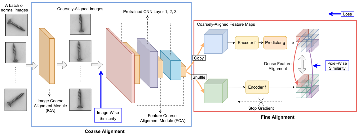
In this section, we demonstrate our novel framework to detect and localize fine-grained anomalies. As indicated in Figure 1, our method consists of a coarse alignment stage and a fine alignment stage. The coarse alignment module first captures and aligns the global context of images. The standardized image features are then passed to the dense representation encoder in for fine-grained self-supervised learning. We construct compact Gaussian distribution from our dense normal features and spot distribution outliers as anomalies.
Coarse Alignment Stage
Image-Level Coarse Alignment (ICA)
The image-level coarse alignment (ICA) aims at regularizing the pixel distribution of normal images: it orients all images in a batch to a similar direction and position for dense comparison. Specifically, we regress the affine transformations on an input image :
| (1) |
Inspired by Spatial Transformer Network (Jaderberg et al. 2015), we adopt its similar architecture to our ICA module, which uses a tiny network to learn the above affine mapping from the original image (denoted by ) to a globally aligned representation (). To train ICA module, we randomly pair the images in a batch and then minimize the distance between them:
| (2) |
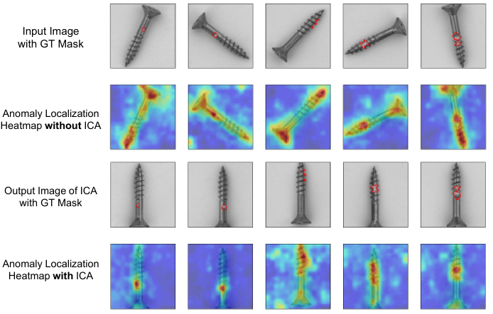
Note that we do not assign any standard orientation or alignment for our module to regress, so it learns a unified position in a self-supervised manner. Each time we random select two images , the loss in Equation 2 supervises the alignment of and toward the reduction of entropy in this system. Thus, given enough iterations, the system reaches a consensus on alignment and the entropy is thus reduced to a local minimum. The results of roughly unified positions are displayed by the coarsely-aligned images in Figure 2.
Feature-Level Coarse Alignment (FCA)
For transformed images in Figure 2, their positions are not strictly aligned to a unified representation. We thus introduce a feature-level coarse alignment (FCA) module to further adjust the high-level image representations. We use a pre-trained ResNet-18 (He et al. 2016) as the feature extractor. As shown in Figure 1, we insert the FCA between succeeding layers to align the embedding distribution with feature-level affine transformation. FCA has a similar implementation as ICA; nonetheless, this module enforces the backbone to extract generalizable features to align positions in a global high-level embedding. The FCA module is only governed by self-supervised loss in the fine alignment stage. The implementation details of image-level and feature-level alignment are in Appendix.
Fine Alignment Stage: Pixel-wise Non-contrastive Learning
Non-contrastive learning is the training of a semantically meaningful normal image representation without leveraging its distance with anomalies. To detect the fine-grained anomalies, we propose the pixel-wise alignment module, which maximizes the feature similarity across every embedding position for all normal images.
As indicated by the Algorithm 1, we first randomly shuffle the minibatch and sample two feature maps. Let denote the two encoded image feature map belonging to two different images from the last FCA. Then, for every position , in these two features, we extract the corresponding feature vectors and . We aim at encoding a unique vector representation for each position in the feature map, as well as narrowing its distribution for all normal images. Thus, we use convolutional operator instead of fully-connected layers in the feature extractor. The vectors are passed to a shared 3-layer 11conv encoder . Only is processed through a 2-layer 11conv predictor to project its feature to the vector space of . Given the two output vectors from the encoder and , we minimize their negative cosine similarity:
| (3) |
where and are the parameters of encoder and predictor, respectively. We conduct the above minimization for and at all positions respectively to densely supervise the positionally-aligned feature distribution.
To avoid model collapsing (Wang and Isola 2020) when training with normal data only, we introduce the stop-gradient operation from (Chen and He 2020). That is, is only allowed to descent backward through the upper branch of the network w.r.t. , and it updates no information of to the encoder . A symmetry operation is applied to further supervise the learning of robust and generalizable features. The aggregated loss for every position thus becomes:
| (4) |
Its implementation is detailed in Algorithm 1. We train the above stages in an end-to-end manner and adjust the weight between coarse and fine alignment with and . Hence, the final loss in our framework is:
| (5) |
is the dominant loss function supervising all parameters and is the auxiliary loss function used to guarantee the convergence of . By optimizing the coarse and fine alignment module collectively, we allow the network to self-adjust and learn meaningful correlations of normal image embeddings.
Anomaly Score Computation in Inference
With the densely extracted features, we model the representation of normal images with the Gaussian distribution for every pixels on feature map following (Defard et al. 2020). We extract the normal image representation at position by concatenating the three pyramid layers of features of CNN at . Let denote the aggregated feature from the CNN for all images of training set. We model a distinctive Gaussian distribution for each pixel on the feature map by:
| (6) |
During inference, we compute the anomaly score by taking the Mahalanobis distances at every pixel between the test images and the normal distribution:
| (7) |
Then, the distance matrix is an anomaly map with dense pixel-wise anomaly scores. A greater score indicates a severer anomalous signal. We thus use the maximum anomaly score map to represent the anomaly score for the entire image.
| Category | DOCC | FCDD | U-S | P-SVDD | SPADE | PaDiM | Cut Paste | Ours | Ours | |
| (WR50) | (WR50) | (R18) | (R18) | (WR50) | ||||||
| texture | carpet | (90.6, -) | (-, 96) | (95.3, -) | (92.9, 92.6) | (-, 97.5) | (-, 98.9) | (93.1, 98.3) | (98.30.4, 98.40.1) | (98.8, 98.5) |
| grid | (52.4, -) | (-, 91) | (98.7, -) | (94.6, 96.2) | (-, 93.7) | (-, 94.9 | (99.9, 97.5) | (97.41.4, 95.70.4) | (98.9, 96.8) | |
| leather | (78.3, -) | (-, 98) | (93.4, -) | (90.9, 97.4) | (-, 97.6) | (-, 99.1) | (100.0, 99.5) | (100.00.0, 98.90.2) | (100.0, 99.2) | |
| tile | (96.5, -) | (-, 91) | (95.8, -) | (97.8, 91.4) | (-, 87.4) | (-, 91.2) | (93.4, 90.5) | (95.41.1, 93.70.7) | (98.8, 96.8) | |
| wood | (91.6, -) | (-, 88) | (95.5, -) | (96.5, 90.8) | (-, 88.5) | (-, 93.6) | (98.6, 95.5) | (99.80.2, 94.20.1) | (99.4, 99.6) | |
| average | (81.9, -) | (-, 93) | (95.7, -) | (94.5, 93.7) | (-, 92.9) | (-, 95.6) | (97.0, 96.3) | (98.20.8, 96.20.3) | (99.20.5, 98.20.2) | |
| object | bottle | (99.6, -) | (-, 97) | (96.7, -) | (98.6, 98.1) | (-, 98.4) | (-, 98.1) | (98.3, 97.6) | (100.00.0, 98.30.0) | (100.00.0, 98.30.0) |
| cable | (90.9, -) | (-, 90) | (82.3, -) | (90.3, 96.8) | (-, 97.2) | (-, 95.8) | (80.6, 90.0) | (94.30.5, 96.70.2) | (95.30.4, 97.50.2) | |
| capsule | (91.0, -) | (-, 93) | (92.8, -) | (76.7, 95.8) | (-, 99.0) | (-, 98.3) | (96.2, 97.4) | (93.21.8, 98.50.6) | (92.52.0, 98.60.8) | |
| hazelnut | (95.0, -) | (-, 95) | (91.4, -) | (92.0, 97.5) | (-, 99.1) | (-, 97.7) | (97.3, 97.3) | (99.80.2, 98.30.1) | (99.90.1, 98.70.1) | |
| metal nut | (85.2, -) | (-, 94) | (94.0, -) | (94.0, 98.0) | (-, 98.1) | (-, 96.7) | (99.3, 93.1) | (99.90.1, 97.10.2) | (99.90.1, 98.20.1) | |
| pill | (80.4, -) | (-, 81) | (86.7, -) | (86.1, 95.1) | (-, 96.5) | (-, 94.7) | (92.4, 95.7) | (94.91.2, 97.20.3) | (94.51.5, 97.30.5) | |
| screw | (86.9, -) | (-, 86) | (87.4, -) | (81.3, 95.7) | (-, 98.9) | (-, 97.4) | (86.3, 96.7) | (89.70.8, 98.70.5) | (90.1, 98.70.4) | |
| toothbrush | (96.4, -) | (-, 94) | (98.6, -) | (100.0, 98.1) | (-, 97.9) | (-, 98.7) | (98.3, 98.1) | (99.90.1, 98.90.0) | (100.00.0, 98.90.0) | |
| transistor | (90.8, -) | (-, 88) | (83.6, -) | (91.5, 97.0) | (-, 94.1) | (-, 97.2) | (95.5, 93.0) | (99.70.1, 98.60.1) | (99.20.3, 98.10.3) | |
| zipper | (92.4, -) | (-, 95.1) | (95.8, -) | (97.9, 95.1) | (-, 96.5) | (-, 98.2) | (99.4, 99.3) | (97.00.5, 97.80.4) | (97.50.5, 98.20.3) | |
| average | (90.9, -) | (-, 91) | (90.9, -) | (90.8, 96.7) | (-, 97.6) | (-, 97.3) | (94.3, 95.8) | (96.80.5, 98.00.2) | (97.00.5, 98.30.3) | |
| average | (87.9, -) | (-, 92) | (92.5, -) | (92.1, 95.7) | (85.5, 96.5) | (95.3, 96.7) | (95.2, 96.0) | (97.30.5, 97.40.2) | (97.70.4, 98.20.3) | |
Experiments
Datasets and Metrics
We perform experiments on two industrial anomaly detection datastes MVTec AD dataset (Bergmann et al. 2019) and BeanTech AD dataset (Mishra et al. 2021). MVTec AD dataset consists of 5354 real-world images with 15 categories, among which 10 of them are objects and the rest 5 are texture classes. BeanTech AD dataset has 3 categories of 2540 images. In both datasets, the training set consists of only normal images, while the testing set has a mixture of both normal and abnormal images. These datasets provides both anomaly types and anomaly masks as test image labels for evaluation. As mentioned previously, the anomalies in these datasets are more fine-grained than those in the academic dataset settings, e.g. the CIFAR-10 (Krizhevsky, Hinton et al. 2009) dataset whose anomaly is defined as different object classes.
Under the one-class classification protocol, we train a model for each category with its respective normal images. The implementation details are listed in Appendix. During inference, we evaluate our method with image-level AUC and pixel-level AUC.
| Categories | AE MSE | AE MSE+SSIM | VT-ADL | Ours (Loc) | Ours (Det) |
|---|---|---|---|---|---|
| 01 | 49.0 | 53.0 | 99.0 | 96.1 | 99.6 |
| 02 | 92.0 | 96.0 | 94.0 | 95.3 | 95.3 |
| 03 | 95.0 | 89.0 | 77.0 | 99.7 | 99.5 |
| average | 78.0 | 79.0 | 90.0 | 97.0 | 98.1 |
| Color Transformation | Spatial Transformation | |||||||
|---|---|---|---|---|---|---|---|---|
| Baseline (det) | Ours (det) | Baseline (loc) | Ours (loc) | Baseline (det) | Ours (det) | Baseline (loc) | Ours (loc) | |
| carpet | 98.5 | 99.3 | 97.4 | 98.7 | 98.1 | 97.3 | 97.9 | 97.7 |
| grid | 90.1 | 95.5 | 93.1 | 94.6 | 91.8 | 95.4 | 93.2 | 95.2 |
| leather | 99.5 | 100.0 | 98.8 | 98.9 | 99.8 | 100.0 | 97.8 | 98.6 |
| tile | - | - | - | - | 96.2 | 97.3 | 91.5 | 94.4 |
| wood | - | - | - | - | 98.7 | 99.1 | 92.9 | 93.8 |
| bottle | 98.9 | 99.9 | 97.2 | 98.1 | 99.6 | 99.7 | 97.4 | 97.5 |
| cable | 92.8 | 95.7 | 96.6 | 97.2 | 93.4 | 96.6 | 95.7 | 96.5 |
| capsule | - | - | - | - | 86.8 | 87.9 | 97.5 | 97.6 |
| hazelnut | 94.2 | 96.4 | 97.1 | 97.4 | 98.2 | 99.8 | 97.5 | 97.7 |
| metal nut | 99.1 | 99.1 | 96.1 | 96.2 | 96.8 | 97.7 | 94.5 | 95.2 |
| pill | 90.8 | 92.2 | 94.3 | 95.8 | 89.7 | 92.2 | 94.8 | 96.9 |
| screw | 89.7 | 90.9 | 98.1 | 98.3 | 66.8 | 70.9 | 95.2 | 97.4 |
| toothbrush | 99.6 | 99.9 | 98.5 | 98.4 | 99.8 | 98.7 | 98.1 | 97.9 |
| transistor | 98.7 | 98.9 | 97.7 | 98.1 | 92.8 | 94.0 | 92.3 | 96.9 |
| zipper | 92.5 | 96.9 | 97.5 | 97.9 | 90.3 | 97.8 | 97.8 | 97.3 |
| average | 95.4 | 97.1 | 96.7 | 97.5 | 93.3 | 95.6 | 95.5 | 96.7 |
Anomaly Detection and Localization for MVTec
In Table 1, we compare our method with the state-of-the-art one-class anomaly detection approaches in MVTec AD dataset, including deep one-class classifier (DOCC) (Ruff et al. 2021), FCDD (Liznerski et al. 2020), uninformed student (U-S) (Bergmann et al. 2020), patch SVDD (Yi and Yoon 2020), SPADE (Cohen and Hoshen 2020), PaDiM (Defard et al. 2020), Cut Paste (Li et al. 2021) under the metrics of image-level AUC and pixel-level AUC, we give the results of the mean and standard deviation of 5 repeated experiments. With our proposed coarse-to-fine non-contrastive learning method, we achieve the best result among all existing works and make notable improvements on both of texture and object defects. Our method surpasses the current state-of-the-art by a margin of 2.1, yieding 97.7 image-level AUC and 98.2 pixel-level AUC. Some results of anomaly localization are visualized in Fig 3 for our method, and more comprehensive results of defect localization are provided in Appendix. We can observe that not only does the anomaly heatmap highlights the object with defect, it also displays intense and fine-grained attention on the small anomalous regions. This proves how our framework focuses precisely on the anomalies.
Anomaly Detection and Localization for BeanTech
In Table 2, we compare our method with the anomaly detection approaches reported in (Mishra et al. 2021) on the BeanTech AD dataset. They applied auto-encoder with MSE loss, auto-encoder with MSE and SSIM loss, and VT-ADL in anomaly localization. We give the results of ResNet-18 and we additionally report the image-level results. Our method achieves the best result among all existing and surpasses the current state-of-the-art by a margin of 7.0, yielding 98.1 image-level AUC and 97.0 pixel-level AUC. This result shows our method’s potential to generalize to new anomalous detection scenarios, where the anomalous data has varied distribution and needs close scrutinization of details.
Performance for Disturbed MVTec
Considering that the current MVTec AD dataset does not contain products with multiple appearances but only has spatially aligned products, we build a new dataset called Disturbed MVTec through various augmentations. We aim at simulating more challenging real life detection situations and verify the robustness and effectiveness of our framework. Specifically, we build two disturbed scenarios with color and spatial transformation, respectively. For the color transformation, we apply random brightness contrast enhancement and limited adaptive histogram equalization in MVTec’s train and test images. For the spatial transformation, we apply random zoom in, zoom out, rotation and flip in the train and test images in MVTec. The examples of these two disturbed datasets and augmentation details are documented in our Appendix. Corresponding experimental results wth ResNet-18 are reported in Table 3. It should be noted that some categories are suitable for color augmentation, especially for the texture classes. For instance, areas of different colors will be treated as anomalies on tile, wood and capsule, so we did not perform color augmentation on them. Moreover, some categories may not suitable do some special kinds of spatial augmentation. For instance, we can not apply vertical flip or rotation in transistor. We can observe that our method performs generally better than the baseline (Defard et al. 2020) under these color and spatial transformations, which shows our framework’s adaptability to complicated settings that simulate the real-world disturbances in industrial images.
Quantitative Analysis on Distribution
To quantify the improvement of distribution compactness in our work, we compare the distance variance score of our method to the baseline (ImageNet pre-trained model). Given a class of total N normal image representations , the distance variance score is calculated by first computing each pixel’s distance to its alignment center:
| (8) |
| (9) |
Then, we get the distance map at every location for all normal images. We compute the distance variance score as the aggregated variance for all distance embedding:
| (10) |
where is the average distance for all images at position . If the distribution of image representations becomes more compact, then would decrease, since the variation in distances between feature vectors to their center should be smaller. We finally aggregate the distance score for all 15 categories in our dataset:
| (11) |
The for the baseline is 0.95, and our method achieves a score of 0.84, which is a 11.6% decrease in the variance score. It thus demonstrates that our method effectively shrinks the feature distributions, while it also keeps the meaningful and discriminating variations in encoding.

Ablation Study
Component-wise Analysis
We investigate the contributions of the main components for our method in Table 4. “Baseline” only uses the ImageNet pre-trained ResNet-18 to model the Gaussian distribution in Equation 6 in inference. “Non-contrastive Learning” is the fine alignment stage to densely maximize the similarity of all images in a batch with the stop-gradient operation. “Coarse Alignment” is the initial image-level and feature-level alignment modules for distribution regularization. The baseline gives less AUC and PRO results comparing to other methods, such as U-S (Bergmann et al. 2020) and PaDiM (Defard et al. 2020). Adding a single non-contrastive learning block improves the image-level AUC to 95.7 and pixel-level AUC to 96.8, which surpasses all previous works. This demonstrates the effectiveness of our designed non-contrastive learning module, because it eliminates the abnormal samples in training and shrinks the distribution of normal samples. Then, adding the coarse alignment module further enhances our advantage over the current state-of-the-art. This is very intuitive, since without first aligning the coarse locations of images, the densely minimized distance among pixels may not be correctly associated. Hence, the ablation study shows the additive effect of each module and the comprehensiveness of our framework.
| Baseline | Dense Non-contrastive Learning | Coarse Alignment | Image-level AUC | Pixel-level AUC | PRO | |
| ICA | FCA | |||||
| ✓ | 92.3 | 95.4 | 89.1 | |||
| ✓ | ✓ | 95.7 | 96.8 | 90.5 | ||
| ✓ | ✓ | ✓ | 96.2 | 97.0 | 90.7 | |
| ✓ | ✓ | ✓ | ✓ | 97.3 | 97.4 | 91.8 |
| carpet | grid | leather | tile | wood | bottle | cable | capsule | |
|---|---|---|---|---|---|---|---|---|
| w/o | 99.3 | 96.3 | 99.5 | 95.9 | 98.8 | 100.0 | 89.4 | 90.4 |
| w | 98.3 | 97.4 | 100.9 | 95.4 | 99.8 | 100.0 | 94.3 | 93.2 |
| hazelnut | pill | metal nut | screw | toothbrush | transistor | zipper | average | |
| w/o | 96.1 | 99.1 | 91.8 | 74.2 | 99.4 | 94.8 | 89.5 | 94.3 |
| w | 99.8 | 99.9 | 94.9 | 89.7 | 99.9 | 99.7 | 97.0 | 97.3 |
Effects of Coarse Alignment Stage
We give the qualitative results of a specific class to show the effects of the coarse alignment stage in Table 5. We can observe that the coarse align stage can improve most of the categories in MVTec AD dataset, especially for “screw”, and we will discuss this improvement is achieved below.
Image-Level Coarse Alignment module
To visualize the result of image-level coarse alignment, we choose the most disordered category screw. As indicated in Figure 2, the screws in dataset have different orientations and positions. The localization heatmap has sparse and distributed attention over the screws, which cannot accurately localize the defects. After passing them through ICA, they are all roughly aligned to the straight-up direction. The heatmap also becomes more focused on the specific defect locations, instead of spreading in different orientations and positions. That is to say, the ICA module narrows the distribution of normal samples and reduces the difficulties in feature learning, which improves the anomaly detection and localization performance.
| Baseline | Layer1 | Layer2 | Layer3 | Image-level AUC | Pixel-level AUC | PRO |
|---|---|---|---|---|---|---|
| ✓ | 96.2 | 96.4 | 90.4 | |||
| ✓ | ✓ | 96.6 | 96.5 | 90.5 | ||
| ✓ | ✓ | 96.7 | 96.6 | 90.7 | ||
| ✓ | ✓ | 96.5 | 96.2 | 90.5 | ||
| ✓ | ✓ | ✓ | ✓ | 97.3 | 97.4 | 91.8 |
Feature-Level Coarse Alignment Module
We investigate the effects of the position of the feature-level coarse alignment module in Table 6. The baseline is the clean backbone without feature-level alignment. We find that inserting FCA after a single feature layer has limited improvement over the baseline, while inserting it in all three layers gives a thorough boost in AUC and PRO. We speculate that although adding FCA in a single layer enables the network to adjust the feature’s positions, it limits the flexibility and reception field of the alignment to a single scope. Adding them to all three layers successively reinforces the feature alignment process and allows the self-supervised signal in Equation 4 to descent backward without information loss.
Conclusion
In this paper, we propose a coarse-to-fine non-contrastive learning framework for unsupervised anomaly detection. The key to our success is the dense non-contrastive learning with coarse alignment and fine alignment module, which encourages the model to learn and narrow down the distribution of normal patterns. Our method achieves high performance on the industrial defect dataset and surpasses the state-of-the-art in both anomaly detection and localization tasks.
Supplementary Material for
Focus Your Distribution: Coarse-to-Fine Non-Contrastive Learning for AnomalyDetection and Localization

Details on Experiments
Implementation Details of two Coarse Alignment modules
Our implementation of the Image-level Coarse Alignment module (ICA) and Feature-level Coarse Alignment module (FCA) is inspired by (Jaderberg et al. 2015). As shown in Figure 4, ICA contains two Convolution layers, two max-pooling layers, and two fully-connected layers. The final FC layer outputs the angle for rotation transformation matrix of input images, which then aligns them to a unified direction.
We develop a self-supervised learning task to train the ICA. Specifically, the ICA loss minimizes the distance between each paired images on one batch in a pixel-wise manner. The pixels are thus enforced to learn shared, representitive position alignment information. We give the details of this self-supervised learning task and its loss function in Algorithm 2.
FCA shares the same the basic structure with ICA, and the only difference between them is the transformation matrix M. In ICA, the matrix M is only used to rotate the image with a single rotation angle, while the M in FCA contains 6 parameters for the affine transformation, including scale, rotation, and translation. Moreover, different from ICA who has a distinctive similarity loss, the supervision signal for FCA is from the non-contrastive learning loss in the fine alignment stage. Therefore, the feature-wise fine alignment gives a full set of high-level alignment, which facilitates the adjustment of features in its downstream non-contrastive learning.
Implementation Details of Training
We use the first three blocks of ImageNet pre-trained ResNet-18 (He et al. 2016) as our backbone network. We train our model on image with one GPU. We update the parameters using momentum SGD with the learning rate of 0.01 for the ICA and 0.0001 for the others. The momentum is set to 0.9, and the batch size is 32. Moreover, we use a single cycle of cosine learning rate decay schedule and L2 weight regularization with a coefficient of 0.00001.
Implementation Details of Disturbed MVTec
For the color transformation, we apply random brightness contrast enhancement and limited adaptive histogram equalization in the train and test images in MVTec. See the examples in Figure 5. We train our model without ICA and FCA in this new color-transformed dataset, the results are reported in the below table. It should be noted that some categories may not suitable do color augmentation, especially for the texture classes. For instance, areas of different colors will be treated as anomalies on tile, wood and capsule, so we did not experiment on them.
For the spatial transformation, we apply random zoom in/out/rotation/flip in the train and test images in MVTec. See the examples in Figure 6. We train our model without ICA and FCA in this new spatial-transformed dataset, the results are reported in the below table. It should be noted that some categories may not suitable do some special kinds of augmentation. For instance, we can not apply flip or rotation in transistor, because transistors are required to be arranged in the specified direction and position.
Optimization Hypothesis in Fine Alignment Stage
We introduce the stop-gradient operation from (Chen and He 2020) to allow training with only normal data and avoid collapsing. We now provide a hypothesis for the mechanism in this non-contrastive learning framework, especially how it helps our model to fit and align compact distribution of normal images.
Optimization Problem Formulation
We hypothesize that our non-contrastive learning implicitly defines a nonparametric clustering algorithm, and the stop-gradient operation thus becomes a decent procedure in the optimization steps. The purpose of our non-contrastive learning module is to regress a representative embedding for a class of normal images along the pixel dimension. This can then be viewed as a single-mode seeking problem for all normal data, from which we identify the most typical features as the mode. At the best case, the mode is the ground truth representation for all normal objects in class .
A natural algorithm for mode seeking is the mean-shift method proposed by (Comaniciu and Meer 2002). That is, let denote N independent random variables, the mean-shift updates through a fixed-point iteration:
| (12) |
where is the kernel that weighs the distance between and . The update continues as converges.
In our setting, let and denote the two corresponding pixels sampled from the feature map and . For each iteration , we define the loss as:
| (13) |
where are parameters for the predictor and encoder .
We use negative cosine similarity as in our paper, but it can be relaxed to any distance measurements. To regress the global minimizer where for all , we perform the gradient descent update of :
| (14) |
With the stop-gradient operation, is treated as a constant and does not back-propagate its gradient to . We can thus interpret as the optimizing target for and to regress toward. Therefore, at each iteration , we update new parameters by treating previous as the approximation for the ground truth representation :
| (15) |
As we aggregate the updates for a batch of images from our random shuffle algorithm, the process of aligning each pair of and toward is equivalent to:
| (16) |
where Z is the random variable for normal image feature maps in a batch. Since we perform the pairing of images by random and assign equal weights to all images, Eq (16) becomes:
| (17) |
where denotes the batch size. We can relax Eq (17) to Eq (12) by adding a flat kernel:
| (18) |
where represents all feature maps in a batch. Then,
| (19) |
Our non-contrastive learning thus becomes an implicitly-defined mean shift algorithm. At each iteration, among all normal images in the training set, the parameters of embedding only shift toward the mean of randomly sampled feature maps from a single batch. By the convergence of fixed-point iteration (Burden and Faires 2011), our method regresses to a mode representation of all normal images given enough training epoches. The scattered feature vectors for embedding thus shrink into a compact distribution where their feature encodings are shared and aligned.
Experimental Results of PRO Metric
The pixel-level AUC score favors over large anomalies. To resolve this, Bergmann et al (Bergmann et al. 2019) introduced the PRO (per-region overlap) metric. For each connected component in the anomaly mask, it plots the mean correctly classified pixel rates over the false positive rate (FPR). The PRO score is the normalized value of the integral of this curve from 0 to 0.3 FPR. A greater PRO score indicates better performance in localizing both obvious and subtle anomalies. We compare our method with existing works under per-region-level in Table 7. We can observe that our method surpasses the state-of-the-art.
Application to Semantic Outlier Detection
We conduct the semantic anomaly detection experiment on CIFAR-10 (Krizhevsky, Hinton et al. 2009) following the protocol in (Golan and El-Yaniv 2018; Sohn et al. 2021), where a single class is treated as normal and the remaining 9 classes are anomalies. We achieves 66.7 AUC, which surpasses some previous works, including OCSVM (Schölkopf et al. 2001), KDE (Parzen 1962), AnoGAN (Schlegl et al. 2017), DeepSVDD (Ruff et al. 2018) and OCGAN (Perera, Nallapati, and Xiang 2019). Still, its performance lags behind some other algorithms that specifically designed for image-level anomaly detection (Perera, Nallapati, and Xiang 2019). This result highlights the difference between fine-grained anomaly detection and image-level defect detection. While the image-level detection focuses on the overall semantic information, our fine-grained anomaly detection aims at detecting subtle anomalies that are usually indiscernible in global semantic context. Such difference suggests that these two detection tasks need different algorithms to target different aspects for the problem.
Anomaly Detection and Localization for Shanghai Tech Campus Dataset
To further investigate the generalization performance of our method, we conduct experiments on Shanghai Tech Campus Dataset. Considering Shanghai Tech is used for video anomaly detection which has 13 sences, we choice 8 sences from them which don’t require the correlation information of the front and rear frames of the video to detect anomaly. We draw images every 5 frames and use all the extracted single frame for training. The results are shown in Table 8.
| Category | U-S (Bergmann et al. 2020) | PaDiM (Defard et al. 2020) | Ours |
| (WR50) | (WR50) | ||
| texture | 79.4 | 93.2 | 93.1 |
| object | 88.9 | 91.3 | 93.0 |
| average | 85.7 | 92.1 | 93.0 |
| Sence | 01 | 02 | 03 | 06 | 09 | 10 | 11 | average |
|---|---|---|---|---|---|---|---|---|
| Pixel-level AUC | 98.8 | 99.0 | 97.5 | 99.4 | 96.0 | 98.1 | 93.9 | 97.5 |

More Anomaly Localization Visualizations
From Figure 7 to Figure 21, we show localization visualizations examples of 10 object and 5 texture categories. We not only show successful cases, but also some failure cases.


References
- Bergman, Cohen, and Hoshen (2020) Bergman, L.; Cohen, N.; and Hoshen, Y. 2020. Deep nearest neighbor anomaly detection. arXiv preprint arXiv:2002.10445.
- Bergman and Hoshen (2020) Bergman, L.; and Hoshen, Y. 2020. Classification-based anomaly detection for general data. International Conference on Learning Representations (ICLR).
- Bergmann et al. (2019) Bergmann, P.; Fauser, M.; Sattlegger, D.; and Steger, C. 2019. MVTec AD – A Comprehensive Real-World Dataset for Unsupervised Anomaly Detection. In Proceedings of the IEEE/CVF Conference on Computer Vision and Pattern Recognition, 9592–9600.
- Bergmann et al. (2020) Bergmann, P.; Fauser, M.; Sattlegger, D.; and Steger, C. 2020. Uninformed students: Student-teacher anomaly detection with discriminative latent embeddings. In Proceedings of the IEEE/CVF Conference on Computer Vision and Pattern Recognition, 4183–4192.
- Burden and Faires (2011) Burden, R. L.; and Faires, J. D. 2011. Numerical analysis.
- Chen et al. (2020) Chen, T.; Kornblith, S.; Norouzi, M.; and Hinton, G. 2020. A simple framework for contrastive learning of visual representations. In International conference on machine learning, 1597–1607. PMLR.
- Chen and He (2020) Chen, X.; and He, K. 2020. Exploring Simple Siamese Representation Learning. arXiv preprint arXiv:2011.10566.
- Cohen and Hoshen (2020) Cohen, N.; and Hoshen, Y. 2020. Sub-image anomaly detection with deep pyramid correspondences. arXiv preprint arXiv:2005.02357.
- Comaniciu and Meer (2002) Comaniciu, D.; and Meer, P. 2002. Mean shift: A robust approach toward feature space analysis. IEEE Transactions on pattern analysis and machine intelligence, 24(5): 603–619.
- Defard et al. (2020) Defard, T.; Setkov, A.; Loesch, A.; and Audigier, R. 2020. PaDiM: a Patch Distribution Modeling Framework for Anomaly Detection and Localization. arXiv preprint arXiv:2011.08785.
- DeVries and Taylor (2017) DeVries, T.; and Taylor, G. W. 2017. Improved regularization of convolutional neural networks with cutout. arXiv preprint arXiv:1708.04552.
- Golan and El-Yaniv (2018) Golan, I.; and El-Yaniv, R. 2018. Deep anomaly detection using geometric transformations. arXiv preprint arXiv:1805.10917.
- Gong et al. (2019) Gong, D.; Liu, L.; Le, V.; Saha, B.; Mansour, M. R.; Venkatesh, S.; and Hengel, A. v. d. 2019. Memorizing normality to detect anomaly: Memory-augmented deep autoencoder for unsupervised anomaly detection. In Proceedings of the IEEE/CVF International Conference on Computer Vision, 1705–1714.
- He et al. (2020) He, K.; Fan, H.; Wu, Y.; Xie, S.; and Girshick, R. 2020. Momentum contrast for unsupervised visual representation learning. In Proceedings of the IEEE/CVF Conference on Computer Vision and Pattern Recognition, 9729–9738.
- He et al. (2016) He, K.; Zhang, X.; Ren, S.; and Sun, J. 2016. Deep residual learning for image recognition. In Proceedings of the IEEE conference on computer vision and pattern recognition, 770–778.
- Hendrycks et al. (2019) Hendrycks, D.; Mazeika, M.; Kadavath, S.; and Song, D. 2019. Using self-supervised learning can improve model robustness and uncertainty. arXiv preprint arXiv:1906.12340.
- Jaderberg et al. (2015) Jaderberg, M.; Simonyan, K.; Zisserman, A.; and Kavukcuoglu, K. 2015. Spatial transformer networks. arXiv preprint arXiv:1506.02025.
- Komodakis and Gidaris (2018) Komodakis, N.; and Gidaris, S. 2018. Unsupervised representation learning by predicting image rotations. In International Conference on Learning Representations (ICLR).
- Krizhevsky, Hinton et al. (2009) Krizhevsky, A.; Hinton, G.; et al. 2009. Learning multiple layers of features from tiny images.
- Li et al. (2021) Li, C.-L.; Sohn, K.; Yoon, J.; and Pfister, T. 2021. CutPaste: Self-Supervised Learning for Anomaly Detection and Localization. arXiv preprint arXiv:2104.04015.
- Liu, Li, and Póczos (2018) Liu, Y.; Li, C.-L.; and Póczos, B. 2018. Classifier Two Sample Test for Video Anomaly Detections. In BMVC, 71.
- Liznerski et al. (2020) Liznerski, P.; Ruff, L.; Vandermeulen, R. A.; Franks, B. J.; Kloft, M.; and Müller, K.-R. 2020. Explainable deep one-class classification. arXiv preprint arXiv:2007.01760.
- Masci et al. (2011) Masci, J.; Meier, U.; Cireşan, D.; and Schmidhuber, J. 2011. Stacked convolutional auto-encoders for hierarchical feature extraction. In International conference on artificial neural networks, 52–59. Springer.
- Mishra et al. (2021) Mishra, P.; Verk, R.; Fornasier, D.; Piciarelli, C.; and Foresti, G. L. 2021. VT-ADL: A Vision Transformer Network for Image Anomaly Detection and Localization. arXiv preprint arXiv:2104.10036.
- Parzen (1962) Parzen, E. 1962. On estimation of a probability density function and mode. The annals of mathematical statistics, 33(3): 1065–1076.
- Perera, Nallapati, and Xiang (2019) Perera, P.; Nallapati, R.; and Xiang, B. 2019. Ocgan: One-class novelty detection using gans with constrained latent representations. In Proceedings of the IEEE/CVF Conference on Computer Vision and Pattern Recognition, 2898–2906.
- Pidhorskyi et al. (2018) Pidhorskyi, S.; Almohsen, R.; Adjeroh, D. A.; and Doretto, G. 2018. Generative probabilistic novelty detection with adversarial autoencoders. NeurIPS.
- Reiss et al. (2021) Reiss, T.; Cohen, N.; Bergman, L.; and Hoshen, Y. 2021. PANDA: Adapting Pretrained Features for Anomaly Detection and Segmentation. In Proceedings of the IEEE/CVF Conference on Computer Vision and Pattern Recognition, 2806–2814.
- Ren et al. (2019) Ren, J.; Liu, P. J.; Fertig, E.; Snoek, J.; Poplin, R.; DePristo, M. A.; Dillon, J. V.; and Lakshminarayanan, B. 2019. Likelihood ratios for out-of-distribution detection. NeurIPS.
- Rippel, Mertens, and Merhof (2021) Rippel, O.; Mertens, P.; and Merhof, D. 2021. Modeling the distribution of normal data in pre-trained deep features for anomaly detection. In 2020 25th International Conference on Pattern Recognition (ICPR), 6726–6733. IEEE.
- Ruff et al. (2021) Ruff, L.; Kauffmann, J. R.; Vandermeulen, R. A.; Montavon, G.; Samek, W.; Kloft, M.; Dietterich, T. G.; and Müller, K.-R. 2021. A unifying review of deep and shallow anomaly detection. Proceedings of the IEEE.
- Ruff et al. (2018) Ruff, L.; Vandermeulen, R.; Goernitz, N.; Deecke, L.; Siddiqui, S. A.; Binder, A.; Müller, E.; and Kloft, M. 2018. Deep one-class classification. In International conference on machine learning, 4393–4402. PMLR.
- Sabokrou et al. (2018) Sabokrou, M.; Khalooei, M.; Fathy, M.; and Adeli, E. 2018. Adversarially learned one-class classifier for novelty detection. In Proceedings of the IEEE Conference on Computer Vision and Pattern Recognition, 3379–3388.
- Schlegl et al. (2017) Schlegl, T.; Seeböck, P.; Waldstein, S. M.; Schmidt-Erfurth, U.; and Langs, G. 2017. Unsupervised anomaly detection with generative adversarial networks to guide marker discovery. In International conference on information processing in medical imaging, 146–157. Springer.
- Schölkopf et al. (2001) Schölkopf, B.; Platt, J. C.; Shawe-Taylor, J.; Smola, A. J.; and Williamson, R. C. 2001. Estimating the support of a high-dimensional distribution. Neural computation, 13(7): 1443–1471.
- Schölkopf et al. (1999) Schölkopf, B.; Williamson, R. C.; Smola, A. J.; Shawe-Taylor, J.; Platt, J. C.; et al. 1999. Support vector method for novelty detection. In NIPS, volume 12, 582–588. Citeseer.
- Seeböck et al. (2016) Seeböck, P.; Waldstein, S.; Klimscha, S.; Gerendas, B. S.; Donner, R.; Schlegl, T.; Schmidt-Erfurth, U.; and Langs, G. 2016. Identifying and categorizing anomalies in retinal imaging data. arXiv preprint arXiv:1612.00686.
- Sohn et al. (2021) Sohn, K.; Li, C.-L.; Yoon, J.; Jin, M.; and Pfister, T. 2021. Learning and Evaluating Representations for Deep One-class Classification. International Conference on Learning Representations (ICLR).
- Sultani, Chen, and Shah (2018) Sultani, W.; Chen, C.; and Shah, M. 2018. Real-world anomaly detection in surveillance videos. In Proceedings of the IEEE conference on computer vision and pattern recognition, 6479–6488.
- Tack et al. (2020) Tack, J.; Mo, S.; Jeong, J.; and Shin, J. 2020. Csi: Novelty detection via contrastive learning on distributionally shifted instances. arXiv preprint arXiv:2007.08176.
- Tax and Duin (1999) Tax, D. M.; and Duin, R. P. 1999. Support vector domain description. Pattern recognition letters, 20(11-13): 1191–1199.
- Tax and Duin (2004) Tax, D. M.; and Duin, R. P. 2004. Support vector data description. Machine learning, 54(1): 45–66.
- Wang and Isola (2020) Wang, T.; and Isola, P. 2020. Understanding contrastive representation learning through alignment and uniformity on the hypersphere. In International Conference on Machine Learning, 9929–9939. PMLR.
- Yi and Yoon (2020) Yi, J.; and Yoon, S. 2020. Patch SVDD: Patch-level SVDD for Anomaly Detection and Segmentation. In Proceedings of the Asian Conference on Computer Vision.
- Yun et al. (2019) Yun, S.; Han, D.; Oh, S. J.; Chun, S.; Choe, J.; and Yoo, Y. 2019. Cutmix: Regularization strategy to train strong classifiers with localizable features. In Proceedings of the IEEE/CVF International Conference on Computer Vision, 6023–6032.