Galaxy-galaxy strong lens perturbations: line-of-sight haloes versus lens subhaloes
Abstract
We rederive the number density of intervening line-of-sight haloes relative to lens subhaloes in galaxy-galaxy strong lensing observations, where these perturbers can generate detectable image fluctuations. Previous studies have calculated the detection limit of a line-of-sight small-mass dark halo by comparing the lensing deflection angles it would cause, to those caused by a subhalo within the lens. However, this overly simplifies the difference in observational consequences between a subhalo and a line-of-sight halo. Furthermore, it does not take into account degeneracies between an extra subhalo and the uncertain properties of the main lens. More in keeping with analyses of real-world observations, we regard a line-of-sight halo as detectable only if adding it to a smooth model generates a statistically significant improvement in the reconstructed image. We find that the number density of detectable line-of-sight perturbers has been overestimated by as much as a factor of two in the previous literature. For typical lensing geometries and configurations, very deep imaging is sensitive to twice as many line-of-sight perturbers as subhaloes, but moderate depth imaging is sensitive to only slightly more line-of-sight perturbers than subhaloes.
Keywords:
dark matter – gravitational lensing: strong1 Introduction
The most fundamental prediction of the cold dark matter (CDM) cosmological model is the existence of a large population of low mass dark matter haloes (Green et al. 2005; Diemand et al. 2007; Springel et al. 2008; Frenk & White 2012; Wang et al. 2020). This feature can be used to test the CDM model rigorously or to distinguish it from models with alternative types of dark matter. For example, the warm dark matter (WDM) model predicts a cutoff in the power spectrum of initial density perturbations, induced by particle free streaming, which translates into a cutoff in the halo mass function at a mass scale that depends on the WDM particle mass (Colín et al. 2000; Lovell et al. 2012; Schneider et al. 2012; Bose et al. 2016).
Recent observations have revealed a line in the X-ray spectra of galaxies and galaxy clusters at 3.5 keV that could result from decay of a WDM particle such as a 7 keV sterile neutrino (Boyarsky et al. 2014; Bulbul et al. 2014, but see Riemer-Sørensen 2016). In this case, the halo mass function today would exhibit a sharp cutoff at a mass, . Thus, this model would be conclusively ruled out if one could demonstrate the existence of a population of haloes below this mass scale. Conversely, the CDM model would be conclusively ruled out if such a population were not found. Haloes that are of mass today were never able to make stars and therefore remain completely dark (see Benitez-Llambay & Frenk 2020; Sawala et al. 2016, and references therein). Such haloes cannot therefore be detected by conventional means but they can, in principle, be detected through their gravitational lensing effects.
Strong lensing systems that exhibit giant arcs or Einstein rings can appear measurably perturbed if any of the light from the source passes sufficiently close to a small dark halo (Koopmans 2005; Vegetti & Koopmans 2009a; Vegetti & Koopmans 2009b; Vegetti et al. 2012; Hezaveh et al. 2016; Li et al. 2016). This is a difficult measurement but applying sophisticated data analysis and modelling tools to high resolution imagery, it is possible to detect small haloes projected near the Einstein radius of the lens and infer their mass (Koopmans 2005; Vegetti & Koopmans 2009a, e.g.). The mass detection limit for dark matter haloes depends on the resolution of the image. With Hubble Space Telescope (HST) imagery, Vegetti et al. 2010 discovered a dark perturber of mass, M⊙, which they interpret as a subhalo in the strong lens system SDSS J0946+1006 (the mass here refers to that of a truncated pseudo-Jaffe density profile). Another dark object of mass, M⊙, was found in a lens galaxy at redshift from even higher resolution imaging using adaptive optics at the Keck telescope (Vegetti et al. 2012).
To constrain the nature of the dark matter with this technique it is, of course, necessary to know the expected number of lensing perturbers in CDM and other models of interest. The perturbers can be either subhaloes of the main lens or “field” haloes that are not part of the main lens but appear projected near its Einstein radius. In what follows, we will refer to the latter as “line-of-sight” or “intervening” haloes or perturbers.
To count the expected number of subhaloes and intervening haloes consistently, Li et al. 2017 derived an effective mass, (), for a line-of-sight halo of mass, . This is determined by fitting a lensing image perturbed by an NFW halo at the lens redshift to the image perturbed by a line-of-sight halo of mass, , at redshift, . In other words, if a subhalo of mass, (), can be detected, a line-of-sight halo of mass, , should also be detected. In this way, one can calculate the effective mass function of all perturbers. Li17 showed that, for CDM, the number of detectable line-of-sight perturbers is 3-4 times larger than the number of subhalo perturbers.
A similar analysis was performed by (Despali et al. 2018, hereafter D18), who derived a fitting formula for by fitting the deflection angle of a lensing system containing a line-of-sight perturber to that of a system containing a subhalo. The analysis was performed for lenses with different image and redshift configurations. In agreement with the results of Li17, they found that the contribution from CDM line-of-sight haloes is about 3 times that from subhaloes for lenses with and , and about 10 times that from subhaloes for lenses with and . Besides, by statistically studying low mass haloes’ perturbation, Çaǧan Şengül et al. 2020 also show that line-of-sight perturbers tend to dominate the signal for systems with a source at redshift higher than 0.5.
The preliminary conclusion that the lensing distortions are dominated by line-of-sight haloes is encouraging because it greatly simplifies the theoretical analysis. Unlike for subhaloes, whose mass function is affected by environmental effects, calculating the mass function of dark central haloes in the mass range of interest - below the threshold for star formation - is straightforward since these haloes have never been affected by baryons. Thus, a standard calculation of the mass function based on dark-matter-only simulations (Frenk et al. 1988) gives very precise results (see Zavala & Frenk 2019, for a recent review).
By contrast, the mass function of subhaloes is determined by a number of processes, such as tidal stripping or tidal shocking, that alter the mass distribution and can destroy the subhalo. To calculate these processes requires modelling the host galaxy in detail, including its baryonic components. This is, of course, a much more complicated problem than simply following the evolution of dark matter haloes. Significant advances, however, have been achieved in recent years with a new generation of cosmological hydrodynamics simulations that can produce realistic galaxy populations (Vogelsberger et al. 2014; Schaye et al. 2015, e.g.). Here, we will make extensive use of the high-resolution hydrodynamics simulation of Richings et al. 2021 of a galaxy cluster and its environment which includes the relevant baryon physics processes.
Li17 and D18 both made an important assumption: that the perturbation induced by a subhalo can always be well fitted by the perturbation induced by a line-of-sight halo with an NFW profile. This assumption, however, may not be exactly true because the deflection angles produced by a line-of-sight halo can be very different from that of a subhalo in certain redshift ranges. Furthermore, these earlier studies did not carry out complete modelling of the lensing process, for example, assuming realistic noise levels, and this may further bias the results.
In this paper, we revisit the importance of the contribution of line-of-sight perturbers by modelling a set of realistic strong lensing mock images. In earlier studies, the comparison of deflection angles was used to decide whether a perturber is detectable or not, through the concept of an “effective mass”. Here we derive the detectable mass threshold for line-of-sight perturbers by directly evaluating the difference in log-likelihood between a model with a perturber and a model without a perturber, using a state-of-the-art strong lens modelling pipeline PyAutoLens11 1 https://github.com/Jammy2211/PyAutoLens (Nightingale et al. 2018; Nightingale et al. 2021b). The new threshold is now directly obtained from modelling image fluxes and thus it is more straightforward and robust, where it takes into account factors from flux modelling processes previously not considered, like the degeneracy between the perturber and the macro model. We also investigate the dependence of the relative contribution of the two types of object on the redshift and the S/N ratio of the observations.
An independent study of the sensitivity function using PyAutoLens is provided by Amorisco et al. 2022. This work reassuringly reaches the same conclusion as us on the dependence of the sensitivity function on the redshift of the perturbing halo, despite using a different approach to calculate the sensitivity function and mock strong lens datasets with different properties. Looking at only line-of-sight haloes, this study highlights the impact that the intrinsic scatter in halo concentrations has on the sensitivity function, and shows that the dependency of the concentration–mass relation on the dark matter model improves strong lensing as a probe of dark matter. In this work, we explicitly include subhalos within the lens galaxy (in addition to line-of-sight haloes), accounting for their different mass function and density profiles due to baryonic physics. Thus, we set out to answer whether the line-of-sight or lens galaxy subhalos dominate the constraints on DM.
The structure of the paper is as follows. In Section 2, we describe how we construct mock lenses, how we compute the sensitivity map and the method we use to translate sensitivity maps into constraints on the halo mass function. In Section 3, we present our results and in Section 4, we summarize our conclusions. Throughout the paper we adopt the Planck cosmological parameters (Planck Collaboration et al. 2016): , and .
2 Method
2.1 Mock Lenses
We construct five sets of mock lenses, including examples with different image configurations, redshifts, noise levels and angular resolution. For simplicity we set the density distribution of all primary lenses to be singular isothermal ellipsoids (SIE),
| (1) |
where and are the Einstein radius and axis ratio of the lens galaxy; is the angular diameter distance between redshifts, and . The lens and source redshifts are marked as, and , respectively. We do not add external shear in the mock lenses. However, when modelling the lens we do include the external shear as part of our mass model (Witt & Mao 1997).
To simulate the source galaxies, we assume a “cored” Sersic density profile:
| (2) |
where is the scale intensity, the effective radius, the Sersic index and a coefficient related to the Sersic index (see Eq. A7 of Trujillo et al. 2004). Compared to the standard Sersic profile, the core model introduces two additional parameters, , which describes the core size, and , which controls how fast the profile approaches constant surface brightness inwards. Throughout our tests we fix and ″. The small core in our model helps to remove potential numerical inaccuracies induced by the cuspy nature of the regular Sersic profile.
The fiducial mock image setup has a nearly complete Einstein ring with the lens galaxy at redshift, , and the source galaxy at . The emission of the lens galaxy is omitted in this work. The mock image has similar angular resolution to HST imaging, where the pixel size is and a Gaussian Point Spread Function (PSF) is assumed where (FWHM of ). For the noise level, we try to set it to be similar to the best cases in the SLACS sample (Bolton et al. 2006), where the maximum S/N in the image pixels is around 40 for a 2000s exposure. We adopt a background sky noise level of 0.1 e, which is estimated from HST images of SLACS lenses. To add noise to each mock image, the background sky is added to the lensed source image, the data is converted to units of counts and Poisson noise values are drawn and added to every pixel. The source intensity is adjusted to make the maximum pixel S/N be 40 and the data is then converted back to e. The lens and source parameters of the fiducial setting is shown in the third column of Table 1.
| Einstein Ring | Quad | ||
| Lens | (x, y) [(″, ″)] | (0.0, 0.0) | (0.0, 0.0) |
| [″] | 1.5 | 1.5 | |
| q | 0.95 | 0.65 | |
| [∘] | 30 | 30 | |
| External Shear | magnitude | 0.0 | 0.0 |
| [∘] | 0.0 | 0.0 | |
| Source | (x, y) [(″, ″)] | (0.1, 0.1) | (-0.05, 0.1) |
| [″] | 0.2 | 0.2 | |
| q | 0.52 | 0.7 | |
| [∘] | 30 | 30 | |
| [e- pix-1 s-1] | 2.2 | 2.3 | |
| 2.5 | 2.0 | ||
| [″] | 0.01 | 0.01 | |
| 2.0 | 2.0 |
Based on this fiducial setup, we also change the appropriate parameters to explore the effects of different image configurations, lens galaxy redshifts, noise levels and angular resolution. We summarize our mock images (without adding any low mass haloes) in Fig. 1, where each setting’s name is labelled in the upper left of each panel. The details of each setting are as follows:
- •
ER-EXP2000 — This is our fiducial setting, a nearly complete Einstein ring with a radius of , corresponding to an Einstein mass of M⊙ within 9.4 kpc.
- •
ER-EXP8000 — It has the same setting as our fiducial mock except the exposure time increases to 8000s, of which the maximum pixel S/N is 80.
- •
ER-EXP2000-LOWZ — The main lens in this case is located at redshift, , while the source is still at . When changing the lens redshift, we keep its Einstein radius (in arcsec) and noise level unchanged. At this redshift, a 1.5″ Einstein radius corresponds to an Einstein mass of M⊙ within 5.5 kpc.
- •
QUAD-EXP2000 — In this setting, we simulate an image with quadruple arcs with the same noise level and angular resolution as the fiducial case. The lens and source parameters of this configuration are listed in the fourth column of Table 1.
- •
ER-CSST — We also simulate a configuration with lens and source properties as in the fiducial case but with the same image resolution as the China Space Station Telescope (CSST). The CSST resolution is slightly worse than for the HST, with a pixel size of and a PSF of (FWHM of ). We note that the hardware design of the CSST is not fully determined yet, so for our purpose here, which is to study purely resolution effects, we assume it has similar noise conditions as the HST except for the resolution. Since the pixel area is 2.25 times larger, the background sky noise is also increased to 0.225 e. The image simulated here may therefore be treated as a pixel binned version of the fiducial mock image using a larger pixel and PSF size of the CSST.
- •
ER-JWST — The image resolution of this case is close to that of James Webb Space Telescope (JWST) images, which have a pixel size of and a PSF of (FWHM of ). Note that now the pixel areas are 0.36 times those of the previous case; the noise is also changed consistently to be 0.036 e.
In Table 2 we summarize the key features of the five mock settings (the quantities of the last three columns are defined in our results part, Sec. 3).

| Label | Configuration | Exposure time (s) | Pixel size | ||||||
|---|---|---|---|---|---|---|---|---|---|
| ER-EXP2000 | Einstein Ring | 0.5 | 1.0 | 2000 | 0.05 | 0.05 | 0.85 | 0.66 | 1.29 |
| ER-EXP8000 | Einstein Ring | 0.5 | 1.0 | 8000 | 0.05 | 0.05 | 2.50 | 1.24 | 2.02 |
| ER-EXP2000-LOWZ | Einstein Ring | 0.22 | 1.0 | 2000 | 0.05 | 0.05 | 0.39 | 0.38 | 1.03 |
| QUAD-EXP2000 | Quad | 0.5 | 1.0 | 2000 | 0.05 | 0.05 | 0.64 | 0.51 | 1.25 |
| ER-CSST | Einstein Ring | 0.5 | 1.0 | N.A.1 | 0.08 | 0.075 | 0.72 | 0.60 | 1.20 |
| ER-JWST | Einstein Ring | 0.5 | 1.0 | N.A.1 | 0.03 | 0.03 | 1.06 | 0.75 | 1.41 |
- 1
For our purpose to investigate how image resolution affect our results, we set them to have equivalent depth of observation as our fiducial setting.
We perturb the images of the mock lenses with two types of objects. One are small-mass dark matter haloes along the line-of-sight and the other are subhaloes within the host halo of the lens galaxy. We model the line-of-sight haloes with spherical NFW profiles using the mass-concentration relation given by Ludlow et al. 2016, which has been shown to match the simulation data very well at the low mass end (Wang et al. 2020).
For subhaloes associated with the lens, their mass profile in the outer parts is modified by environmental effects such as tidal stripping. N-body simulations have shown that the density of these subhaloes drops dramatically beyond a truncation radius (Gao et al. 2004, e.g.). In this paper we simulate the subhalo profile using a truncated NFW (tNFW) profile (Baltz et al. 2009, see Eq. A.26A.33 of),
| (3) |
where is the scale mass, is the scale radius and is the truncation radius. The total mass of the subhalo, , can be written as (Baltz et al. 2009, Eq. A.29 of),
| (4) |
where .
We derive the mean relation between , and using the high-resolution hydrodynamical simulation by Richings et al. 2021. This is a zoom, high resolution resimulation of a halo with (the mass within , the radius where the enclosed density is 200 times the critical density of the Universe) of M⊙ at selected from the eagle simulation volume (Schaye et al. 2015) and resimulated with 17 times better gas mass resolution than eagle, M⊙, and about 100 times better dark matter mass resolution than eagle, M⊙. Such high resolution allows us to resolve the internal structure of subhaloes more massive than 108 M⊙. Haloes were identified using the friends-of-friends algorithm (Davis et al. 1985) and subhaloes using the SUBFIND algorithm (Springel et al. 2001); the density profiles of subhaloes in the mass range M⊙ were fit with the tNFW formula to derive the values of , and .
Since in actual observations, only subhaloes around the Einstein radius matter, we only select subhaloes whose projected positions fall in an annular region between and from the lens centre to derive the relations between , and . To improve the statistics, we rotated the simulated halo 10000 times at random. For the mock lenses at and we make use of the snapshots at and respectively. To make sure the derived relations are not dominated by any particular subhalo, e.g. by one very close to the Einstein radius in 3D, we carry out bootstrap tests whereby we repeat the same procedure 200 times and each time we derive the linear relations from a random re-sample of all subhaloes. The linear relation is computed by minimizing a defined as:
| (5) |
where , are the linear relation slope and intercept, is the coordinate of the -th data point and is the number of times the -th data point is repeated in the sample. We then take the median linear relations from the 200 tests to model the subhaloes.
Taking the snapshot at as an example, in Fig. 2, we plot the values of , and for subhaloes as blue circles. The area of each circle reflects how many times each subhalo fell on the annular region around the Einstein radius, which is taken as a weight for the point when deriving the linear relation. For this lens system we find,
| (6) |
For the lens at we find,
| (7) |
where the errors are the 1 scatter determined from the bootstrap resampling.

In Fig. 3, we show the interior mean surface density profiles of tNFW subhaloes of mass M⊙ for two different lens redshifts, and the same profiles of central haloes of mass M⊙ for two different lens redshifts. The profiles of the tNFW model were derived from the mean linear relations between , , and described above. Clearly, the tNFW profiles are more compact and have higher amplitude than the NFW profiles of the same mass.

2.2 Sensitivity Mapping
A process called sensitivity mapping is performed to quantify the detectability of a perturbing halo that is nearby a strongly lensed source. One begins by modeling a strong lens dataset to infer an accurate model for the lens’s mass and source’s light (Nightingale et al. 2019). Using this model, one can then simulate a new realization of the strong lens which includes a dark matter perturber at a given position in the image-plane and with an input mass and redshift. This simulated dataset assumes the same image resolution and PSF of the true dataset and also has consistent signal-to-noise properties.
The mock dataset is now fitted with two lens models: (i) a lens mass model which does not include a dark matter perturber and; (ii) a lens mass model which does. By comparing a goodness-of-fit measure of each model-fit (e.g. the maximum log likelihood value) one therefore quantifies how sensitive the lens dataset is to a dark matter perturber, given its input location and mass. If the lens model including the perturber has a much improved goodness-of-fit compared to the model which does not, the perturber was necessary to fit the data accurately, indicating that the strong lens data is sensitive to perturbers at the location and with that mass. If the goodness-of-fits are comparable, the perturber does not improve the lens model and therefore it is too far from the lensed source or too low mass to be detectable.
It is necessary to perform two full fits to each mock dataset, to infer the maximum log likelihood of each model, for two reasons. First, the image fluxes we are fitting have noise and thus the maximum likelihood model may not be the true input model (Amorisco et al. 2022, although see). Second, due to the existence of a small perturber in the mock data and the possible degeneracy between it and the main lens mass, when fitting a model without a small perturber, the maximum likelihood model is offset with respect to the true input and can only be found via a full fit.

By repeating this process on a grid of perturber (,) location, mass and redshift one produces a sensitivity map. In this work, we assume a grid of 27 steps in the and directions, and a grid of 25 steps in redshift between = 0.02 and = 0.98. For a given object, its angular size decreases with redshift, so the angular size of the sensitive region also decreases with redshift. To save computational resources, we decrease the angular size of the explored region as the redshift increases. Furthermore, for the same reason, rather than exploring a grid of mass values, we look for the lowest value of the perturber’s mass that corresponds to the goodness-of-fits threshold of detection by a binary search algorithm (in scale). The mass boundaries for the binary search are 106 M⊙ and 1011 M⊙ and the stop criterion for the iteration is that . For every grid cell, we simulate a new strong lens dataset and fit it with the two lens models described above using the nested sampling algorithm dynesty (Speagle 2020). For efficiency, we use tight priors on every model-fit that exploit our knowledge of what values of lens mass model and source model were used to when simulating the data. This could negatively impact dynesty’s estimate of the Bayesian evidence, therefore we opt to simply compare maximum log likelihood values when producing a sensitivity map. At the end, the “sensitivity map” is a grid of (, , , ), which means that a perturber at (, , ) is detectable when it has a mass over the threshold mass, . Please note when fitting the mock image with a lens mass model including a pertuber model, the perturber model’s redshift is fixed to be while its position and mass are free (the concentration follows Ludlow et al. 2016 which is a function of and .). Fig. 4 summarizes the procedure of computing for at (, , ). Our method is conceptually analogous to that of Amorisco et al. 2022, albeit there are differences in the fitting algorithm used.
2.3 Detection threshold
Previous studies (Li et al. 2016; Despali et al. 2018) have derived the detection threshold of a line-of-sight perturbing halo by directly modelling the lensing effect of a subhalo, i.e. a perturber at the redshift of the lens. If a line-of-sight halo of mass, , best fits the lensing effect of a subhalo of mass, , then this is defined as the effective mass of the line-of-sight halo. If a line-of-sight halo has an effective mass larger than the detection threshold for the subhalo, it is considered detectable. However, in many cases, the line-of-sight halo at redshift is not a good description of the image perturbation. As a result, although one can always find a particular value of for a line-of-sight halo that gives the smallest in the fit of the image distortion generated by the subhalo, the two models are not equivalent.
In Fig. 5, we show how the deflection angles produced by our lens are altered by the addition of a perturbing halo. The main lens is an singular isothermal sphere (SIS) located at , at the centre of the image, and the source is at . The upper panel shows the deflections caused by a M⊙ NFW halo located on the main lens plane; the colour indicates the amplitude of the deflections (in units of ″) and the arrows mark their directions. In this case there are no non-linear multi-plane lensing effects, and so the change in the deflection angles due to a perturbing halo are just the deflection angles of the perturbing halo itself, which point towards the perturber’s centre. In the lower panel we plot the change in the total deflection angles when a M⊙ NFW halo at perturbs the lensing due to the main lens (subtracting the total deflection angle with the deflection caused only by the main lens). Because of multi-plane lensing effects (Schneider et al. 1992; Fleury et al. 2021) the change in the deflection angles are no longer isotropic about the perturber centre (Gilman et al. 2019; He et al. 2022). Tracing from the observer backwards, the deflection of light rays by the perturber alters where those rays intersect the main lens plane, which in turn alters the deflection angles those rays receives from the main lens. It is clear that the lensing effects of line-of-sight perturbers at different redshifts cannot be reproduced by appropriately scaled subhaloes since the deflection patterns in the two cases are completely different. Note that the mass of the line-of-sight perturber in the lower panel was chosen to best reproduce the deflection angle field in the annulus between 1.0″to 2.0″of the case in the top panel with a M⊙ halo in the main lens plane (following Eq. 15 in D18), so according to Li17 and D18, the perturbers in the two panels have the same “effective mass”, but clearly they have quite different effects.
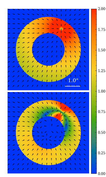
Degeneracies between the effects of the low-mass perturber and the main lens can also affect our estimation. As suggested in Fig. 5, the deflection angles far from the perturber’s centre can be easily absorbed by slightly shifting and stretching the main lens. Furthermore, the degeneracies between the effects of perturbers and the main lens galaxy can be different at different redshifts due to their distinct deflection patterns, making the problem even more complicated.
In order to take into full account the complex effects discussed above, in this paper we no longer compare deflection angles as Li17 and D18 did. Instead, to quantify the lensing effects of perturbers at different redshifts we directly fit image fluxes, a procedure that more closely reproduces what would happen on real data. We now define a new threshold for detection through the log-likelihood22 2 The log likelihoods are defined using a natural (base ) logarithm. improvement brought about by including a perturber when fitting lensing images. Specifically, we first fit the mock image with only a main lens and record the maximum log-likelihood value. We then fit the same image with a model containing both a main lens and a perturbing halo and record the log-likelihood of the best-fit model as well. If the log-likelihood difference between the two fits is larger than a pre-established threshold, we consider the perturber to be detectable.
In the tests we have carried out, the uncertainty in the modelling comes exclusively from the statistical noise in the image data. The log-likelihood difference can be directly related to a significance level, with a log-likelihood difference of 10 roughly corresponding to 4 significance. Note that in real observations, a threshold based on the log-likelihood difference or the Bayesian evidence might not be readily related to the true significance of a detection due to the possible presence of various systematic effects in the data and analysis method (Vegetti et al. 2012; Ritondale et al. 2019).
2.4 Number density of perturbers
For each mock lens, we calculate the number of line-of-sight perturbing haloes within a radius of 3 arcsec. The total number of line-of-sight perturbers with a mass in the range in a light cone corresponding to the pixel can be written as,
| (8) |
where is the halo mass function at redshift (Sheth et al. 2001, e.g.) and
| (9) |
where is the total solid angle corresponding to the areas on the redshift plane of that are sensitive to perturbers more massive than .
For comparison, we also calculate the number of detectable subhaloes for each mock image. For CDM, high-resolution N-body simulations have shown that the mass function of subhaloes follows a power law (Springel et al. 2008). Thus, the cumulative perturber density of subhaloes in the mass range, , in a host halo of mass, , may be written as,
| (10) |
where (Springel et al. 2008; Gao et al. 2012) and is a normalization parameter that depends on and can be determined from cosmological simulations. In this work, we estimate this normalization using the same simulation (Richings et al. 2021) that we used to extract the density structure of subhaloes.
To obtain a sufficiently large sample of subhaloes within the region of interest in order to derive the subhalo mass function, we follow the same strategy as before: we rotate the lens 10000 times, and only select those subhaloes that fall on the region of interest in projection. We compute the average number of subhaloes of mass M⊙ for each projection. To obtain an estimate on the error, we repeat the same procedure 200 times, each time resampling from all the subhaloes in the simulation before projecting along 10000 different lines-of-sight. We take the median value and 1 limits as our estimate. Assuming , for a lens at , we derive the normalization (from the snapshot at ) to be . For a lens at , we derive the normalization (from the snapshot at ) to be .
To ensure that our result based on this one particular simulated halo is not an outlier, we compute the normalisation of the subhalo mass function from haloes in the Eagle simulation in a similar way as above. Due to the poorer resolution of Eagle, when calculating the normalisation we only count subhaloes of mass M⊙. We select haloes in Eagle with mass within 0.1 dex of that of the main halo used in this study and apply the same method to compute . For , there are 78 haloes and arcsec-2, where the errors indicate the (34%) scatter. For , there are 63 Eagle haloes and arcsec-2. We see that the number of Eagle subhaloes around halos of a given mass has a large scatter and there can be differences of times within Eagle itself. At , the vaule of obtained for the halo analysed here is high compared to the distribution in Eagle, while at , the results are in even better agreement. In conclusion, the value of derived in this work is comparable to values for Eagle haloes and our results based on one particular resimulation should be representative.
3 Results
In Fig. 6 we show the sensitivity function for our mock lens images as a function of redshift. Each sub-panel displays a map of (see colour bar) for line-of-sight haloes placed at a given redshift plane, for 5 redshifts. In all cases, the source is at and the lens at , except in the third row, where the lens is at . For all mock lenses, the threshold mass of a detectable perturber is lowest near the lens redshift and raises rapidly towards both higher and lower redshifts; however, the general pattern of the sensitivity maps remains similar at each redshift. This pattern varies considerably from one lensing system to another. Visually, it appears similar to the corresponding pattern of the lensing image. The value of is lowest in the region where the surface brightness is highest and highest in the region where there is no light. Although the sensitivity maps for different systems are quite different, the trend of their evolution with redshift is similar.
The ability to detect low-mass dark haloes increases significantly with the exposure time of the imaging. For our fiducial 2000s exposures, our lensing systems are sensitive to line-of-sight perturbers of mass M⊙ only around the lens redshift. For 8000s, however, perturbers of mass M⊙ can be detected over a much broader redshift range, from to . In the bottom two rows of Fig. 6, we show the sensitivity function for the imaging quality achievable with the CSST and JWST, which have different resolutions. We find that with a lower image resolution, CSST lensing images are still sensitive to perturbers of mass M⊙, although the overall sensitivity is somewhat lower than with HST resolution. While for the JWST resolution imaging, the sensitivity is higher.
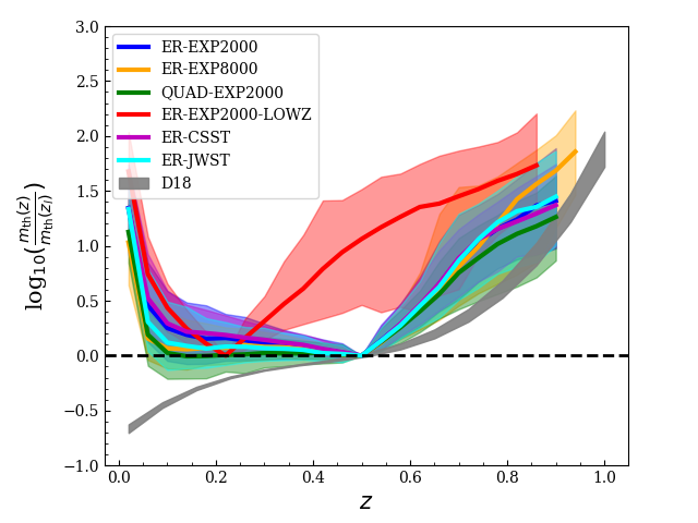
We now turn our attention to the all-important question of whether the distortions to the Einstein rings are dominated by line-of-sight perturbers or by subhaloes. We trace the position of each pixel on the image plane at a series of redshifts and calculate the threshold mass for detection, . In Fig. 7, we plot the ratio, , as a function of redshift, , for our different mock lensing systems. The colour bands are the regions enclosing 70% of the pixels, while the means are shown as solid lines. For comparison, we also plot the relation and scatter derived by D18 in grey. In D18 (as well as in Li17), a line-of-sight halo at lower redshift is easier to detect than a halo of the same mass at the lens redshift. Our new calculations predict the different behaviour. For all configurations, the detection threshold mass increases with . For lenses at redshift , the detection threshold for line-of-sight haloes at is dex higher than for haloes at .
To predict the number density of detectable subhaloes, we calculate sensitivity maps for subhaloes with truncated NFW profiles, as described in Sec. 2.1. In Fig. 8, we compare sensitivity maps for subhaloes (right) to those for line-of-sight haloes placed at the lens redshift of the same lensing system (left). The maps on the left are the same as in the subpanels of Fig. 6 at the corresponding (lens) redshift, while the right panels show the detection limits for subhaloes. The mass of an NFW halo is defined to be , while the mass of the subhalo (tNFW) is defined as the total mass given by Eq. 4. As expected, the threshold mass for detecting a subhalo is lower than that for detecting an NFW halo of the same mass by about 0.5 dex, because a subhalo is much more compact than a halo of the same mass. In the following calculations, we will use the sensitivity maps for the tNFW haloes to estimate the number of detectable subhalo perturbers
In the left panel of Fig. 9, we show, as solid lines, the expected cumulative number of detectable line-of-sight perturbers derived, as a function of redshift; different colours correspond to different systems. We can see that the number of detections rises sharply around the lens redshift and then becomes flat. For the two different mock lenses at , with a 2000s exposure (blue and green lines), 0.85 and 0.64 line-of-sight haloes can be detected per lens. The differences between the two configurations are small, which may be due to the fact that the two mock images have a similar number of high S/N pixels. For the lens at , the number of expected detections decreases to about 0.39 per lens (red line), which is of that of the lenses. Fig. 9 also shows that a high S/N ratio (blue line) helps reveal low-mass perturbers: if the exposure time increases to 8000s, the number of detectable line-of-sight perturbers increases to 2.5 per lens. We also see that by increasing the image resolution, the detectability of small perturbers increases. With CSST resolution only 0.72 line-of-sight perturber can be detected per lens, but with a higher resolution as the JWST, the detectable number increases to 1.06 per lens.
On the right panel of Fig. 9, we show the relative importance of line-of-sight haloes and subhaloes. According to our calculation, for mock lenses at , the predicted number of detectable line-of-sight haloes is about 1.3 times the number of detectable subhaloes. For the low redshift mock, , the line-of-sight halo contribution is lower and close to that of subhaloes. For the high S/N mock, the relative importance of line-of-sight haloes increases, such that it becomes 2.0 times the number of detectable subhaloes.



4 Discussion and Conclusion
In this study we have revisited a key question relevant to the search for low-mass haloes in strong lensing systems: what is the relative contribution to the sensitivity function of line-of-sight (main) haloes versus subhaloes in the lens. The main difference between this and previous works is that, instead of fitting the deflection angle map or an idealized image set, we have quantified the expected number of line-of-sight perturbers by means of realistic modelling carried out with the PyAutoLens lensing package on a set of mock lensing images with realistic levels of noise. Contrary to previous work, we find that the lensing effect of a line-of-sight perturber is largest if the perturber is located near the lens redshift, and the strength of the signal decreases rapidly as the redshift difference between the perturber and the lens plane increases. Two reasons account for the difference: firstly, previous work assumed that the effects of a perturber at one redshift could be accounted for by a perturber at a different redshift, while Fig. 5 demonstrates that the effects can be quite different because of multi-plane lensing effects; secondly, previous work did not take into account the degeneracy between the main lens and the small halo in the fitting process, whereby changes to the main lens model can absorb a significant part of the small perturber’s lensing signal. Our calculation shows that the contribution from line-of-sight haloes is still important, but does not dominate the total number of detectable perturbers for most of our mock lenses as was previously thought: previous studies overestimated the expected total number of perturbers.
In a sense, our new results present an unwanted challenge for the interpretation of future detections of low-mass haloes. Unlike the line-of-sight field dark matter haloes of interest (whose masses are below the minimum required to make a galaxy) which are unaffected by baryons and thus retain their pristine structure, subhaloes are changed by their environment, e.g. tidal striping and disruption. A detailed quantification of these processes needs understanding in detail the structure of the galaxy, including its baryonic component. This requires full modelling of galaxy formation such as that presented by Richings et al. 2020 for a lens system of the kind in which we are interested for low-mass halo and subhalo detection.
In this work we have assumed, for simplicity, that the distribution of line-of-sight haloes is not correlated with the lens host halo. In reality, line-of-sight haloes are more strongly, and anisotropically clustered around the region of the host halo than average (Richings et al. 2021). In a recent paper, Lazar et al. 2021 investigated the number density of line-of-sight perturbers in the simulations from the FIRE33 3 http://fire.northwestern.edu and IllustrisTNG44 4 https://www.tng-project.org projects; they find that the number of haloes correlated with the lens is about 35% larger than average, in agreement with the results of Richings et al. 2021. Future work aimed at constraining the nature of the dark matter from strong lensing data will need to take this sort of correlation into account.
One caveat of our work is that we do not consider the scatter in the mass-concentration relation. For a halo or subhalo of a given mass, the higher the concentration, the higher the central density and lensing signal. A recent study by Minor et al. 2021 shows that this effect can introduce a bias of 3 for a subhalo of mass M⊙ and 6 for one of mass M⊙. In a more recent study, Amorisco et al. 2022 show that the scatter in the mass-concentration relation boosts the detection of line-of-sight perturbers and helps distinguish between CDM and WDM. A halo of mass less than but of higher than average concentration may still produce a strong enough lensing signal to be detected and vice versa. When the halo or subhalo mass function rises at the low mass end, the effect of scatter in the mass-concentration relation can boost the number of detectable perturbers significantly, helping distinguish different dark matter models. We remind our readers that the results discussed here are for analyses of resolved lensing systems where the sources are extended. Effects of mass-concentration relation and multi-plane lensing have been taken into account in previous similar studies on constraining low-mass perturbers’ abundance in lensing systems with an unresolved source (Gilman et al. 2019; Gilman et al. 2020).
In this work, we also show that the ability to detect low-mass haloes increases with the exposure time of the image. For example, increasing the exposure time from 2000s to 8000s, increases the number of total detectable perturbers by a factor of 2. At face value, deeper imaging may seem not quite as efficient an observing strategy as observing more lenses. However, longer exposure times crucially increase the sensitivity to haloes of lower mass, which are important in constraining the identity of the dark matter.
Software Citations
This work used the following software packages:
- •
- •
- •
- •
- •
- •
- •
- •
- •
- •
- •
5 Acknowledgements
We thank the anonymous referee for insightful comments that helped us improve our paper. RL acknowledge the support of National Nature Science Foundation of China (Nos 11988101,11773032,12022306)), the science research grants from the China Manned Space Project (No CMS-CSST-2021-B01, CMS-CSST-2021-A01), the support from K.C.Wong Education Foundation. QH, AA, CSF and SMC acknowledge support from the European Research Council (ERC) through Advanced Investigator grant DMIDAS (GA 786910). We also acknowledge support from the STFC Consolidated Grant ST/T000244/1. JWN and RJM acknowledge support from the UKSA through awards ST/V001582/1 and ST/T002565/1; RJM is also supported by the Royal Society. AR is supported by the ERC through Horizon2020 grant EWC (AMD-776247-6). NCA is supported by an STFC/UKRI Ernest Rutherford Fellowship, Project Reference: ST/S004998/1. This work used the DiRAC@Durham facility managed by the Institute for Computational Cosmology on behalf of the STFC DiRAC HPC Facility (www.dirac.ac.uk). The equipment was funded by BEIS capital funding via STFC capital grants ST/K00042X/1, ST/P002293/1, ST/R002371/1 and ST/S002502/1, Durham University and STFC operations grant ST/R000832/1. DiRAC is part of the National e-infrastructure.
Data availability
The data underlying this article will be shared on reasonable request to the corresponding author.
References
- Amorisco et al. (2022) Amorisco N. C., et al., 2022, MNRAS, 510, 2464
- Astropy Collaboration et al. (2013) Astropy Collaboration et al., 2013, A&A, 558, A33
- Baltz et al. (2009) Baltz E. A., Marshall P., Oguri M., 2009, J. Cosmology Astropart. Phys., 2009, 015
- Benitez-Llambay & Frenk (2020) Benitez-Llambay A., Frenk C., 2020, MNRAS, 498, 4887
- Bolton et al. (2006) Bolton A. S., Burles S., Koopmans L. V. E., Treu T., Moustakas L. A., 2006, ApJ, 638, 703
- Bose et al. (2016) Bose S., Hellwing W. A., Frenk C. S., Jenkins A., Lovell M. R., Helly J. C., Li B., 2016, MNRAS, 455, 318
- Boyarsky et al. (2014) Boyarsky A., Ruchayskiy O., Iakubovskyi D., Franse J., 2014, Physical Review Letters, 113, 251301
- Bulbul et al. (2014) Bulbul E., Markevitch M., Foster A., Smith R. K., Loewenstein M., Randall S. W., 2014, ApJ, 789, 13
- Colín et al. (2000) Colín P., Avila-Reese V., Valenzuela O., 2000, ApJ, 542, 622
- Davis et al. (1985) Davis M., Efstathiou G., Frenk C. S., White S. D. M., 1985, ApJ, 292, 371
- Despali et al. (2018) Despali G., Vegetti S., White S. D. M., Giocoli C., van den Bosch F. C., 2018, MNRAS, 475, 5424
- Diemand et al. (2007) Diemand J., Kuhlen M., Madau P., 2007, ApJ, 667, 859
- Diemer (2018) Diemer B., 2018, The Astrophysical Journal Supplement Series, 239, 35
- Fleury et al. (2021) Fleury P., Larena J., Uzan J.-P., 2021, J. Cosmology Astropart. Phys., 2021, 024
- Foreman-Mackey (2016) Foreman-Mackey D., 2016, The Journal of Open Source Software, 1, 24
- Frenk & White (2012) Frenk C. S., White S. D. M., 2012, Annalen der Physik, 524, 507
- Frenk et al. (1988) Frenk C. S., White S. D. M., Davis M., Efstathiou G., 1988, ApJ, 327, 507
- Gao et al. (2004) Gao L., White S. D. M., Jenkins A., Stoehr F., Springel V., 2004, MNRAS, 355, 819
- Gao et al. (2012) Gao L., Navarro J. F., Frenk C. S., Jenkins A., Springel V., White S. D. M., 2012, MNRAS, 425, 2169
- Gilman et al. (2019) Gilman D., Birrer S., Treu T., Nierenberg A., Benson A., 2019, MNRAS, 487, 5721
- Gilman et al. (2020) Gilman D., Du X., Benson A., Birrer S., Nierenberg A., Treu T., 2020, MNRAS, 492, L12
- Green et al. (2005) Green A. M., Hofmann S., Schwarz D. J., 2005, J. Cosmology Astropart. Phys., 8, 003
- He et al. (2022) He Q., et al., 2022, MNRAS, 511, 3046
- Hezaveh et al. (2016) Hezaveh Y. D., et al., 2016, ApJ, 823, 37
- Hunter (2007) Hunter J. D., 2007, Computing in Science & Engineering, 9, 90
- Koopmans (2005) Koopmans L. V. E., 2005, MNRAS, 363, 1136
- Lazar et al. (2021) Lazar A., Bullock J. S., Boylan-Kolchin M., Feldmann R., Çatmabacak O., Moustakas L., 2021, MNRAS, 502, 6064
- Li et al. (2016) Li R., Frenk C. S., Cole S., Gao L., Bose S., Hellwing W. A., 2016, MNRAS, 460, 363
- Li et al. (2017) Li R., Frenk C. S., Cole S., Wang Q., Gao L., 2017, MNRAS, 468, 1426
- Lovell et al. (2012) Lovell M. R., et al., 2012, MNRAS, 420, 2318
- Ludlow et al. (2016) Ludlow A. D., Bose S., Angulo R. E., Wang L., Hellwing W. A., Navarro J. F., Cole S., Frenk C. S., 2016, MNRAS, 460, 1214
- Minor et al. (2021) Minor Q., Kaplinghat M., Chan T. H., Simon E., 2021, MNRAS,
- Murray et al. (2013) Murray S. G., Power C., Robotham A. S. G., 2013, Astronomy and Computing, 3, 23
- Nightingale & Dye (2015) Nightingale J. W., Dye S., 2015, MNRAS, 452, 2940
- Nightingale et al. (2018) Nightingale J. W., Dye S., Massey R. J., 2018, MNRAS, 478, 4738
- Nightingale et al. (2019) Nightingale J. W., Massey R. J., Harvey D. R., Cooper A. P., Etherington A., Tam S. I., Hayes R. G., 2019, MNRAS, 489, 2049
- Nightingale et al. (2021a) Nightingale J. W., Hayes R. G., Griffiths M., 2021a, Journal of Open Source Software, 6, 2550
- Nightingale et al. (2021b) Nightingale J. W., et al., 2021b, Journal of Open Source Software, 6, 2825
- Planck Collaboration et al. (2016) Planck Collaboration et al., 2016, A&A, 594, A13
- Price-Whelan et al. (2018) Price-Whelan A. M., et al., 2018, AJ, 156, 123
- Richings et al. (2020) Richings J., et al., 2020, MNRAS, 492, 5780
- Richings et al. (2021) Richings J., Frenk C., Jenkins A., Robertson A., Schaller M., 2021, MNRAS, 501, 4657
- Riemer-Sørensen (2016) Riemer-Sørensen S., 2016, A&A, 590, A71
- Ritondale et al. (2019) Ritondale E., Vegetti S., Despali G., Auger M. W., Koopmans L. V. E., McKean J. P., 2019, MNRAS, 485, 2179
- Sawala et al. (2016) Sawala T., et al., 2016, MNRAS, 456, 85
- Schaye et al. (2015) Schaye J., et al., 2015, MNRAS, 446, 521
- Schneider et al. (1992) Schneider P., Ehlers J., Falco E. E., 1992, Gravitational Lenses, doi:10.1007/978-3-662-03758-4.
- Schneider et al. (2012) Schneider A., Smith R. E., Macciò A. V., Moore B., 2012, MNRAS, 424, 684
- Sheth et al. (2001) Sheth R. K., Mo H. J., Tormen G., 2001, MNRAS, 323, 1
- Speagle (2020) Speagle J. S., 2020, MNRAS, 493, 3132
- Springel et al. (2001) Springel V., White S. D. M., Tormen G., Kauffmann G., 2001, MNRAS, 328, 726
- Springel et al. (2008) Springel V., et al., 2008, MNRAS, 391, 1685
- Trujillo et al. (2004) Trujillo I., Erwin P., Asensio Ramos A., Graham A. W., 2004, AJ, 127, 1917
- Van Rossum & Drake (2009) Van Rossum G., Drake F. L., 2009, Python 3 Reference Manual. CreateSpace, Scotts Valley, CA
- Vegetti & Koopmans (2009a) Vegetti S., Koopmans L. V. E., 2009a, MNRAS, 392, 945
- Vegetti & Koopmans (2009b) Vegetti S., Koopmans L. V. E., 2009b, MNRAS, 400, 1583
- Vegetti et al. (2010) Vegetti S., Koopmans L. V. E., Bolton A., Treu T., Gavazzi R., 2010, MNRAS, 408, 1969
- Vegetti et al. (2012) Vegetti S., Lagattuta D. J., McKean J. P., Auger M. W., Fassnacht C. D., Koopmans L. V. E., 2012, Nature, 481, 341
- Virtanen et al. (2020) Virtanen P., et al., 2020, Nature Methods, 17, 261
- Vogelsberger et al. (2014) Vogelsberger M., et al., 2014, MNRAS, 444, 1518
- Wang et al. (2020) Wang J., Bose S., Frenk C. S., Gao L., Jenkins A., Springel V., White S. D. M., 2020, Nature, 585, 39
- Witt & Mao (1997) Witt H. J., Mao S., 1997, MNRAS, 291, 211
- Zavala & Frenk (2019) Zavala J., Frenk C. S., 2019, Galaxies, 7, 81
- Çaǧan Şengül et al. (2020) Çaǧan Şengül A., Tsang A., Diaz Rivero A., Dvorkin C., Zhu H.-M., Seljak U., 2020, Phys. Rev. D, 102, 063502
- van der Walt et al. (2011) van der Walt S., Colbert S. C., Varoquaux G., 2011, Computing in Science Engineering, 13, 22