[datatype=bibtex] \map[overwrite=false] \step[fieldsource=note] \step[fieldset=addendum, origfieldval, final] \step[fieldset=note, null]
Extension of
the J-PARC Hadron Experimental Facility
- Third White Paper -
Abstract
The J-PARC Hadron Experimental Facility was constructed with an aim to explore the origin and evolution of matter in the universe through the experiments with intense particle beams. In the past decade, many results on particle and nuclear physics have been obtained at the present facility. To expand the physics programs to unexplored regions never achieved, the extension project of the Hadron Experimental Facility has been extensively discussed. This white paper presents the physics of the extension of the Hadron Experimental Facility for resolving the issues in the fields of the strangeness nuclear physics, hadron physics, and flavor physics.
Preface
Toward realization of the extension of the Hadron Experimental Facility at J-PARC, this White Paper presents the physics to be newly developed in the extended facility.
The extension project has been discussed extensively among particle and nuclear physics communities in Japan since the early stage of the J-PARC construction. In the user community of the Hadron Experimental Facility, Hadron Hall Users’ Association (HUA), a committee for the study of the facility extension was formed in August, 2015, and made two White Papers as arXiv.1706.07916 [nucl-ex] and arXiv.1906.02357 [nucl-ex]. In September, 2020, we organized a Task Force (TF) under HUA aiming at early realization of the extension through further discussions on the important physics features at the extended facility. The task force was composed of three groups based on three core lines of research conducted at J-PARC: strangeness nuclear physics (HIHR/K1.1-TF), hadron physics (K10-TF), and flavor physics (KL2-TF). We held a series of workshops in the first half of 2021, and substantial interest and support were given to the extension project at the international level. Physics case deeply discussed in the workshops is summarized as this third White Paper. On August 10,11,17,25, 2021, the extension project was reviewed by an international committee of ’Focused review committee of Hadron Experimental Facility Extension’ formed under J-PARC PAC, for which this third White Paper was used as an input document. Detailed information on the extension project can be found in HUA’s home page, where documents related to the project, links to the workshops and review, and supporting letters for the project are available:
https://www.rcnp.osaka-u.ac.jp/~jparchua/en/hefextension.html
We wish this third White Paper strongly pushes forward the extension project of the Hadron Experimental Facility at J-PARC.
1 Executive Summary
1.1 Introduction
The Japan Proton Accelerator Research Complex (J-PARC) is a multi-purpose accelerator facility located in Tokai village, Japan [985, 986]. The aim of J-PARC is to promote a variety of scientific research programs ranging from the basic science of particle, nuclear, atomic, and condensed matter physics and life science to the industrial application and future nuclear transmutation using intense particle beams. Among them, the Hadron Experimental Facility focuses on particle and nuclear physics to explore the origin and evolution of matter in the universe, using the primary 30 GeV proton beam and secondary beams of pions, kaons, and muons. With the intense hadron beams, a wide variety of experiments are performed to approach the open questions in the universe:
- •
Is there new physics beyond the Standard Model?
- •
How is the matter-antimatter asymmetry that resulted in the matter-dominance universe generated?
- •
What is the origin of the hadron mass that weights 99.9% of the visible matter in the universe ?
- •
How are hadrons built from quarks and gluons?
- •
What is the origin of the short-range part of the nuclear force which plays essential roles in formation of atomic nuclei?
- •
What are the properties of high-density nuclear matter that may exist in compact stars in the universe ?
To answer these questions based on fundamental physical laws, the following three core lines of research have been conducted at J-PARC.
The first is strangeness nuclear physics. It aims at elucidation of the matter containing strange quarks. Observation of a neutron-star merger event by gravitational wave at LIGO and Virgo and subsequent multi-messenger astronomical observations have provided information on the equation of states (EOS) of nuclear matter and the synthesis of heavy chemical elements [987]. However, the dense nuclear matter deep inside the neutron stars still remains unknown because the properties of the nuclear matter and interactions among the constituent particles, hadrons, have not been fully understood. Today, aiming to clarify the whole picture of neutron stars, a wide range of scientific programs have been developed from microscopic to macroscopic approaches. In particular, since hyperons are predicted to play an important role in such dense environment, the interactions involving hyperons in the nuclear matter should be determined with microscopic approaches. At J-PARC, the world’s leading research on hypernuclear physics has been conducted and provided important information, together with precise measurements of hyperon-nucleon scattering, to understand baryon-baryon interactions extended to the strangeness sector.
The second is hadron physics. It aims to understand the structure of hadrons as composite systems of quarks and gluons. Due to non-perturbative nature of QCD, hadrons are considered to be formed through complex non-trivial dynamics of quantum fields. The most important features are confinement and the spontaneous breaking of chiral symmetry, leading to the emergence of constituent quarks as quasi-particles and pions as Nambu-Goldstone bosons. Furthermore, various flavor contents with different masses result in a variety of structures including exotic hadrons, and in the flavor dependent structure of hadronic matter there should be a key for understanding deep inside the neutron stars. There are many issues not yet solved systematically. The high-intensity hadron beams in the energy region of several GeV at J-PARC enable us to explore precise spectroscopy of hadrons with quarks. A framework to explain and predict various hadron properties will be established.
The third is flavor physics. It aims at discovery of new physics beyond the Standard Model (SM). Since no clear evidence for new physics is found in vigorous direct searches at LHC, flavor physics in intensity frontier plays a particularly important role today. The decay, which directly breaks the CP symmetry, is utilized as a probe. Since the SM predicts the branching ratio to be with small theoretical uncertainties [988], it provides us with a hit of new physics that the measured branching ratio differ from the branching ratio predicted in the SM.
Charged lepton flavour violation is a definite sign for new physics beyond the SM. The COMET experiment, aiming to search for coherent neutrino-less conversion of a muon to an electron of in muonic atoms ( conversion), provides us with a window on new physics with the world’s highest sensitivity.
Since the first delivery of the proton beam to the Hadron Experimental Facility in January 2009, experiments were carried out and many fruitful results have been obtained. In order to expand the programs of particle and nuclear physics to the regions that have not been explored, more beam lines are indispensable. In the present Hadron Experimental Facility, a single production target is placed and is shared with a limited number of secondary beam lines due to the limited space of the present hall. About 50% of the primary protons from the J-PARC Main Ring (MR) are used to produce secondary particles at the target, and the remaining protons are transported to the beam dump [989].
The extension of the facility by adding more production targets and installing new secondary beam lines will substantially expand our research opportunities with the following merits.
Enabling new measurements that are not possible at the present facility.
For the strangeness and hadron physics, construction of a ‘high-intensity high-resolution beam line’ and a ‘high-momentum mass-separated beam line’, with unprecedented capabilities, are highly anticipated to solve unsettled problems in nuclear physics. In particular, a solution to the “hyperon puzzle” is expected by high-precision spectroscopy of -hypernuclei that provides ultra-precise binding-energy measurements in a wide mass range for the study of density-dependent and interactions. In rare kaon decays, the extension of the hall enables us to optimize the flux of kaons and neutrons in the ‘neutral beam line’. With an extraction angle of 5 degrees, which had originally been chosen to be 16 degrees in the existing KL beam line at the present hall due to space limitations [990], we will be able to utilize a more intense kaon beam and thereby dramatically increase the experiments’ sensitivity.
More efficient and flexible operation of the facility.
The existing K1.8 beam line is optimized for studying nuclei with two strange quarks, whereas the studies of nuclei with a single strange quark are performed at the branch line (K1.8BR) [991]. These two beam lines share the upstream part, and cannot be operated at the same time. With a new dedicated ‘low-momentum beam line’, which provides kaon beams with higher intensity and better quality (e.g., better ratio), experiments can be performed simultaneously. More flexible operation can also be realized for high momentum beams: the existing primary proton beam line (high-p) and a new ‘high-momentum mass-separated beam line’. These beam lines, operated simultaneously, can accommodate the increasing demands from a wide variety of physics programs.
The extension project further promotes the three core research lines: strangeness nuclear physics, hadron physics, and flavor physics. With the world’s highest-intensity beams available at the Hadron Experimental Facility, we aim to achieve the following goals:
- •
to elucidate at microscopic level neutron stars’ EOS, by solving the hyperon puzzle,
- •
to reveal baryon structure built from quarks and gluons, utilizing spectroscopic studies of strange and charm baryons, and
- •
to investigate new physics beyond the Standard Model through rare kaon decays.
The capability of the facility will be enhanced and enable us to reach the objective
- •
to increase the diversity of world class physics programs at J-PARC on the basis of newly constructed unique beam lines.
To maintain the world’s leading position of the Hadron Experimental Facility in the several-GeV energy region, the diversity is of vital importance. The operation with more production targets is also essential to realize sustainable researches in the accelerator-based science in the future.
The extension project has been long discussed since the early stage of the J-PARC construction. This is because when the whole J-PARC project was approved in 2000, the size of the Hadron Facility was reduced to almost a half of the original design due to budgetary limitation. The nuclear physics community in Japan has requested realization of the extension with the highest priority, and the particle physics community has also expressed its importance. The project was selected as one of 31 important projects in “Japanese Master Plan for Large Research Projects 2020” by the Science Council of Japan, and then selected as one of 15 projects in “Roadmap 2020 for promoting large scientific research projects” by Ministry of Education, Culture, Sports, Science and Technology (MEXT) of Japan.
In the user community, Hadron Hall Users’ Association (HUA), extensive discussions on the project have been made. A committee was organized under HUA for planning of the extension of the hadron experimental facility and made the first White Paper on the Hadron Experimental Facility extension project as arXiv.1706.07916 [nucl-ex] [992]. It includes the roles of the project, overview of the facilities, and how particle and nuclear physics can utilize it to attack the relevant open questions. Concering details of the beam lines and many experimental lines of research to be carried out in the project, the second White Paper was issued as arXiv.1906.02357 [nucl-ex] [993], based on the discussions in ‘International workshop on the project for the extended hadron experimental facility’ held in March 2018. The plan of the project has been updated and revised since then, by taking into account recent progress of research in the Hadron Experimental Facility together with the global situation in the field of particle and nuclear physics. In 2020, we organized a task force under HUA, and held a series of workshops in the first half of 2021 to deepen discussions on the important physics features at the extended Hadron Experimental Facility. In this report, we summarize the updates.
This report is organized as follows. The present status of the Hadron Experimental Facility is briefly introduced in subsection 1.2. The scientific goals and expected achievements in the extension project are summarized for each subject in Sec. 1.3 together with the present situation: what is the problem to be solved, what has been achieved at the present facility so far, and how to approach the goal at the new project. A facility overview of the extended Hadron Experimental Facility is described in Sec. 1.4, and the expected timeline of the project is given in Sec. 1.5. Finally, we review the global situation of accelerator-based physics in Sec. 1.6 to clarify the position of the J-PARC Hadron Experimental Facility in the world. In Sec. 2 and later, we describe details of each experimental program planned at the new beam lines in the extended facility.
1.2 Present Status of the Hadron Experimental Facility

In the present Hadron Experimental Facility, a low-momentum charged-kaon beam line (K1.8/K1.8BR), a neutral-kaon beam line (KL), and a primary proton beam line (high-p) are being operated. A new primary beam line for a muon-to-electron conversion experiment (COMET) will also be ready for operation in 2022. Figure 1 shows a layout of the present experimental hall 11 1 To operate the K1.1 beam line in Fig. 1, it is required to build the downstream part as well as the experimental area at the south side of the experimental hall. There is spatial overlap between the high-p and K1.1 beam lines. It takes more than nine months to get the experiment ready for the changeover, during which other beam lines in the hall cannot be operated due to the regulation of radiation protection. . Primary protons are slowly extracted from the Main Ring accelerator (MR) and transported to the experimental hall (MR-SX operation) [994]. Kaons produced at the primary target (T1) are extracted to each secondary kaon beam line. The primary protons are also delivered to the high-p and COMET beam lines by branching off the protons in the switchyard at the upstream of the T1 target.
Table 1 summarizes the experiments classified as “completed”, “ongoing”, “forthcoming”, and “planned” with their results. Published results are also listed in the table. Their highlights are as follows.
- Search for penta-quark via the reaction (E19)
-
Upper limits on the production cross section and width of were obtained [995]. - Search for H via the 6Li reaction (E10)
- bound state via the reaction (E27)
-
A like structure was observed [998]. - -ray spectroscopy of He and F (E13)
- bound state via the 3He reaction (E15)
-
A bound state was observed [1001]. - hypernucleus via the 12C reaction (E05)
-
A Be hypernuclear state was observed [1002]. - resonance via the d reaction (E31)
-
The scattering amplitude below the threshold was obtained [1003]. - Double-strangeness hypernuclei with hybrid emulsion method (E07)
- Measurement of the scatterings (E40)
-
Differential cross sections of the elastic scattering were derived with drastically improved precision [1007]. - Study of the decay (E14 KOTO)
-
A single-event sensitivity of was achieved with the dataset taken in 2016-2018. Three events were observed in the signal region, which was consistent with the number of expected background events, [1008]. The physics data taking continues to improve the sensitivity by installing new counters to reduce background events.
A review paper of the nuclear physics programs at the Hadron Experimental Facility was published [1009].
| Experiment | beam line | Beam | Status | |
| particle | ||||
| E03 | Measurement of X-rays from -atom | K1.8 | completed | |
| E05 | Spectroscopic study of -hypernucleus, Be, via the 12C reaction | K1.8 | completed [1002, 1010] | |
| E07 | Systematic study of double strangeness system with an emulsion-counter hybrid method | K1.8 | completed [1004, 1005, 1006] | |
| E08 | Pion double charge exchange on oxygen at J-PARC | K1.8 | planned | |
| E10 | Production of neutron-rich -hypernuclei with the double charge-exchange reactions | K1.8 | completed [1011, 996] | |
| E13 | Gamma-ray spectroscopy of light hypernuclei | K1.8 | completed [999, 1000] | |
| E18 | Coincidence Measurement of the Weak Decay of and the three-body weak interaction process | K1.8 | forthcoming | |
| E19 | High-resolution search for pentaquark in reactions | K1.8 | completed [1012, 995] | |
| E22 | Exclusive Study on the Lambda-N Weak Interaction in A=4 Lambda-Hypernuclei | K1.8 | planned | |
| E26 | Direct measurements of mass modification in A reaction and decays | K1.8 | planned | |
| E27 | Search for a nuclear bound state in the d reaction | K1.8 | completed [1013, 998] | |
| E40 | Measurement of the cross sections of scatterings | K1.8 | completed [1007] | |
| E42 | Search for -dibaryon with a large acceptance hyperon spectrometer | K1.8 | completed | |
| E45 | 3-body hadronic reactions for new aspects of baryon spectroscopy | K1.8 | forthcoming | |
| E70 | Proposal for the next E05 run with the - spectrometer | K1.8 | forthcoming | |
| E75 | Decay Pion Spectroscopy of Produced by -hypernuclear Decay | K1.8 | planned | |
| E15 | A search for deeply-bound kaonic nuclear states by in-flight 3He reaction | K1.8BR | completed [1014, 1015, 1016, 1001] | |
| E31 | Spectroscopic study of hyperon resonances below threshold via the reaction on deuteron | K1.8BR | completed [1017, 1003] | |
| E57 | Measurement of the strong interaction induced shift and width of the 1st state of kaonic deuterium at J-PARC | K1.8BR | planned | |
| E62 | Precision spectroscopy of kaonic helium 3 X-rays | K1.8BR | completed [1018, 1019] | |
| E72 | Search for a narrow resonance using the reaction with the hypTPC detector | K1.8BR | forthcoming | |
| E73 | and mesonic weak decay lifetime measurement with 3,4HeH reaction | K1.8BR | planned | |
| E80 | Systematic investigation of the light kaonic nuclei - via the in-flight 4He reactions | K1.8BR | planned | |
| Experiment | beam line | Beam | Status | |
| particle | ||||
| E14 | Proposal for Experiment at J-PARC | KL | ongoing [1020, 1021, 1022, 1008] | |
| E16 | Electron pair spectrometer at the J-PARC 50-GeV PS to explore the chiral symmetry in QCD | high-p | ongoing | |
| E50 | Charmed baryon spectroscopy via the reaction | high-p | planned | |
| E79 | Search for an dibaryon resonance | high-p | planned | |
| E29 | Study of in medium mass modification for the meson using meson bound state in nucleus | K1.1 | planned | |
| E63 | Proposal of the 2nd stage of E13 experiment | K1.1 | forthcoming | |
| E36 | Measurement of and Search for heavy sterile neutrinos using the TREK detector system | K1.1BR | completed [1023] | |
| E21 | An Experimental Search for Conversion at a Sensitivity of with a Slow-Extracted Bunched Beam | COMET | forthcoming | |
As of June 2021, a beam power of 64.5 kW was achieved with a 2.0 s beam duration in a 5.2 repetition cycle, which corresponds to 7.01013 protons per pulse. The present production target system T1, which is composed of a gold rod cooled by an indirect water-cooling system [1024, 1025], is allowable to 95 kW under the 5.2 repetition cycle. Further improvement of the accelerator beam power is being planned; the upgrade of the MR main-magnet power supplies will realize a MR-SX power over 100 kW by operation with a higher repetition rate than that at the present. To receive the beam of higher power, a new production target system up to 150 kW is also being developed, which employs a rotating-disk target with a direct helium-gas-cooling system.
1.3 Scientific Goals in the Extension Project
1.3.1 Elucidation of neutron star matter microscopically through solving the hyperon puzzle
A so-called “hyperon puzzle” is the difficulty to reconcile the astronomical observations of two-solar-mass neutron stars [1026, 1027] with the presence of hyperons in their interiors predicted by nuclear physics; the hyperon presence makes the equation of state (EOS) softer and thereby the maximum mass of neutron stars is incompatible with the observations.22 2 The high momentum tail due to the nucleon-nucleon short-range correlations (SRC) also affects the EOS of neutron stars. The observed dominance of the SRC pairs compared to the pairs is a clear consequence of the nucleon-nucleon tensor correlation. In Jlab experiments, the high-momentum fraction was measured for both proton and neutron [1028]. In 208Pb, the fraction of the high-momentum proton increased, whereas the fraction of the high-momentum neutron decreased. In the neutron star, this SRC increases the average kinetic energy of protons, while it decreases that of neutrons. This decrease of the neutron’s energy makes the symmetry energy softer. Therefore, the SRC is another source for softening the EOS [1029]. If the bare interaction with the short-range repulsive core and the tensor force is used in microscopic approaches such as the variational method, the SRC effect is expected to be taken into account in the calculation. In the neutron star density, the dominant source of repulsive interaction is three-body repulsive force. However, the SRC should also be discussed together in future. The solution of this problem requires a mechanism providing an additional repulsion between baryons to make the EOS stiffer. Such additional repulsion would be described by two-body baryon-baryon interactions and three-body baryon-baryon-baryon interactions including hyperons, which give essential effects in dense nuclear matter. We need much more comprehensive information on the hyperon-nucleon () and hyperon-hyperon () interactions both in the free space and in the nuclear medium. To determine the strength of the hyperonic three-body repulsive forces, it is vital to measure the binding energies () of -hypernuclei precisely in a wide mass-number region. The information on the density-dependent interaction can be obtained from them.
At the Hadron Experimental Facility, experiments on hypernuclei have been proposed and performed to determine the strengths of the baryon-baryon interactions extended to the strangeness sector. The and interactions have been and will be derived with world’s most accurate measurements of the hypernuclei at the existing K1.8 beam line using the reaction. The interactions in the free space will be precisely obtained by scattering experiments planned at the new K1.1 and high-p beam lines. The strength of the - coupling will also be precisely obtained by spectroscopic studies of light neutron-rich hypernuclei and precision measurements of charge symmetry breaking in hypernuclei. The -ray spectroscopy of hypernuclei is a powerful tool to determine low-lying level structure of hypernuclei precisely. The differential cross-section measurements of the and scatterings are essential to determine the - coupling in the free space, because the - coupling could be modified in the nuclear medium. These experiments have been and will be performed at K1.8 and K1.1.
To obtain information on the hyperonic three-body repulsive force, however, we need innovative measurements of hypernuclei with unprecedented precision in the wide mass-number region. Such three-body effect affects the binding energy particularly in heavy hypernuclei. The effect is expected to be from a few hundred keV to a few MeV, depending on the two-body interaction. In the heavy hypernuclei, the couples to a core nucleus of various one-hole excited states having a small energy difference with each other. It results in several hypernuclear states with narrow energy spacings of typically a few hundred keV. In order to determine the binding energies by separating each state and to provide accurate information including the three-body effect, a new spectroscopic method should be introduced. In fact, the past experiment at KEK could not separate each state due to a limited energy resolution of 2 MeV (FWHM). New experiments proposed at the newly constructed HIHR beam line can break through the situation. The binding energy can be determined with a resolution of a few hundred keV (FWHM) from the light (He) to heavy (Pb) hypernuclei, by using the missing-mass spectroscopy by using high-intensity pion beams and thin nuclear targets. The systematic high-precision spectroscopy from light to heavy hypernuclei provides essential data to extract the repulsive hyperonic three-body force effect through theoretical studies based on the realistic interaction determined from the scattering experiments to be preformed at K1.1. The -ray spectroscopy provides us with additional information to determine the level structure of hypernuclei, in particular for the heavy hypernuclei where the level spacing could be narrower than the HIHR resolution. The -ray information will be also used to interpret the binding energy spectrum obtained by HIHR. The density-dependent interaction effects also appear in the mass-number dependence of the level spacing between the and states, because the averaged nuclear density which the feels in the orbital is expected to be different for different mass number. The level spacing between and can be determined with a few keV accuracy from -ray spectroscopy using germanium detectors.
Only after combining the realistic and interactions with the hyperonic three-body force strength obtained from the comprehensive studies in hypernuclear physics, a realistic EOS can be established to solve the hyperon puzzle.
1.3.2 Revelation of baryon structure built by quarks and gluons through spectroscopic studies of strange and charm baryons
Quantum chromodynamics (QCD) has succeeded in describing the interactions between quarks and gluons, and hadron properties. However, low energy phenomena such as the formation of hadrons are not clearly explained yet, because perturbative calculations do not work in the low energy regime.
At the present Hadron Experimental Facility, experimental approaches to investigate the in-medium properties of mesons are being made. They are expected to provide crucial information on the spontaneous breaking of chiral symmetry associated with the mass generation of hadrons, which is the most important feature of QCD at low energy. Various investigations of in-medium meson properties have been and will be performed, such as the precise measurement of the spectral functions of vector mesons in medium at High-p and systematic measurement of the light kaonic nuclei at K1.8BR.
Spectroscopy of baryons (baryon spectroscopy) is another important approach to investigate how QCD works at low energy, which is to be explored at J-PARC. In particular, a basic question ”how quarks build hadrons” has yet to be answered clearly. It is vital to understand dynamics of effective degrees of freedom, that are constituent quarks and Nambu-Goldstone bosons, brought by the non-trivial gluon field at low energy. Spectroscopy of baryons with heavy flavors provides a good opportunity to investigate interactions and correlations of the effective degrees of freedom in hadrons. In excited baryons containing a heavy quark, the correlation between a quark pair inside the baryon is expected to be enhanced. It is referred as a diquark correlation. There are longstanding arguments if the diquark correlations play roles on baryon structure and are related to the diquark condensations at highly dense quark matter, though they are not settled yet.
At the energy of J-PARC, excited baryons with a charm quark or multi strange quarks are appropriate. An experiment to study the diquark correlation in charmed baryons (denoted as ) is planned at the beam line with secondary high-momentum pions.
Spectroscopy of baryons is planned at the new K10 with intense, separated kaons to investigate the diquark correlation in the strangeness sector, and to explore an unknown field of excited baryons (denoted as ) 33 3 A pilot experiment on baryons [1030] is planned also at with identifying kaons from pions of intensity more than 2 orders of magnitude, which will be able to provide basic information on the production cross sections as well as possible background processes prior to the further investigation at K10..
By introducing quarks with different flavors having different masses in a baryon, a relative motion between two quarks in a diquark and a collective motion of the diquark to the other quark are kinematically separated. We will employ the the and reactions since the production cross sections reflect the above-mentioned diquark motions [1031, 1032]. It is noted that we can populate and from the ground states up to highly excited states systematically since they are identified in the missing mass spectra. By measuring decay particles in coincidence with a populated state, we can measure the branching ratio (decay partial width) easily, which carries information on the internal structure of the excited baryon. This is an advantage in fixed-target experiments.
Further investigations of the quark correlation can be performed at the new K10 beam line, via the simplest systems - baryons. The baryons are unique because the pion coupling is rather weak compared to the other hadrons including and quarks, and thereby the quark-gluon dynamics will be directly reflected to the exited state . However, since the production cross sections of is expected to be small in case of the reaction, the investigations can only be preformed using intense and separated kaon beams available at K10.
1.3.3 Investigating new physics beyond the Standard Model through rare kaon decays
The Standard Model (SM) in particle physics successfully describe how elementary particles interact with each other. The last missing particle in the SM, a Higgs particle, was discovered in 2012 by the ATLAS and CMS experiments at the LHC [1033, 1034]. However, there still remains many questions that cannot be explained by the SM such as the matter-dominant universe and the low mass of the Higgs boson, and thereby the searches for new physics beyond the SM have been pursued intensively. Since direct production of new particles would not be discovered so easily in LHC, the role of flavor physics experiments, which investigate new physics at a high energy scale through rare phenomena by using intensity frontier machines, become more important.
At the KL beam line in the present hall, the KOTO experiment searches for the rare kaon decay . This decay directly violates CP symmetry. The branching ratio is highly suppressed, and is predicted to be with small theoretical uncertainties at a level of 2% [988]. Thus, this decay is one of the most sensitive probes to search for new physics. The KOTO experiment set the most stringent upper limit on the branching ratio to be at the 90% confidence level with the dataset taken in 2015 [1021]. The sensitivity of was achieved with the dataset taken in 2016-2018. Three events were observed in the signal region, which was consistent with the number of expected background events, [1008]. With newly installed counters to reduce background events, the KOTO experiment continues to take physics data and will reach a sensitivity better than in 3-4 years. However, the achievable sensitivity will be eventually saturated. It is desirable to design a new experiment that can observe the sufficient number of SM-predicted events for the measurement of the decay.
In the extended facility, the KOTO step-2 experiment plans to build a new neutral kaon beam line (KL2) with a smaller extraction angle than that for the KOTO experiment to increase the flux and prepare a longer detector to extend the signal region and improve the signal acceptance. The KOTO step-2 experiment aims to measure the branching ratio of the decay, with a beam intensity of 100 kW for three snow-mass-years, in an accuracy of 27% by observing 35 SM events with a signal-to-background ratio of 0.63.
The breaking of time-reversal (T) symmetry will also be investigated at the K1.1BR beam line by measuring the transverse polarization of the muon from the decay. T violation, connected to CP violation through the CPT theorem, is an important key to solve the matter-antimatter asymmetry in the universe.
The observables from the kaon rare decays, together with the measurements in factories such as the Belle II experiment, play an important role to investigate the flavor structure in new physics.
1.4 Extended Hadron Experimental Facility and Its Realization
In the extension project, the construction of the following new beam lines will expand the potential for particle and nuclear physics programs at J-PARC.
- •
HIHR beam line: High-intensity and high-resolution charged meson beam line for high-precision spectroscopy of -hypernuclei. The beam line will adopt state-of-the-art technology of the dispersion-matching method, and enable us to operate more than pions / spill up to 2 GeV/ with the beam momentum resolution of . The missing-mass resolution of a few 100 keV (FWHM) will be achieved corresponding to the -hypernuclei mass determination with several ten keV accuracy, which has never been realized so far.
- •
K10 beam line: High-momentum (2–10 GeV/) charged meson and anti-proton beam line for investigations of strangeness physics and charm physics. The beam line will provide separated secondary beams with the higher momentum than any existing beam lines. The high-momentum particle separation will be realized by two-stage RF separators.
- •
K1.1 beam line: Low-momentum (1.2 GeV/) charged meson beam line optimized for investigations of strangeness physics. High-purity and high-intensity secondary particles will be available by using two-stage electrostatic separators. A branched beam line (K1.1BR) which focuses on experiments using stopped kaons will also be prepared.
- •
KL2 beam line: High-intensity neutral meson beam line dedicated to measure the branching ratio of the rare decay . The extraction angle of 5 degrees will be adopted, instead of 16 degrees in the existing beam line, to increase the yield while keeping the ratio of kaons and neutrons which could become a source of background events.
Figure 2 shows a layout of the extended Hadron Experimental Facility together with the present facility. The size of the experimental area will be twice larger and a new production target (T2) will be placed. The new beam lines will be connected from the T2 target station. A test beam line is planned to be constructed in the experimental area that has previously been used for the KL experiment. In the extended experimental hall, five beam lines (plus the test beam line) in total will be operated simultaneously. The specifications of the beam lines for both the present and the extended Hadron Experimental Facility are summarized in Table 2. By using the two production targets, effective utilization of intense primary protons will be realized.

| Particles | Momentum | Intensity | Characteristics | |
| beam lines in the present hadron experimental facility | ||||
| K1.8 | 1.0 – 2.0 GeV/c | 106 /spill (1.8) | mass separated | |
| K1.8BR | 1.1 GeV/c | 5105 /spill (1.0) | mass separated | |
| KL | 2.1 GeV/c in ave. | 107 /spill | 16∘ extraction angle | |
| high-p | 1010 /spill | primary beam (30 GeV) | ||
| 31 GeV/c | 107 /spill | secondary beam | ||
| COMET | for experiment | |||
| beam lines in the extended area | ||||
| K1.1 | 1.2 GeV/c | 4105 /spill (1.1) | mass separated | |
| K1.1BR | 0.7 – 0.8 GeVc | 1.5105 /spill | mass separated | |
| HIHR | 2.0 GeV/c | 2108 /spill (1.2) | mass separated | |
| 10 better | ||||
| K10 | 10 GeV/c | 7106 /spill | mass separated | |
| KL2 | 5 GeV/c in ave. | 4107 /spill | 5∘ extraction angle | |
| optimized | ||||
In the original plan of the extension project, the size of the experimental area was three times larger than the present area and two new production targets (T2 and T3) were considered to be placed, as described in the first and second white papers. Thereafter we have reconsidered the extension plan to reduce the cost, by decreasing both the size of the experimental area and the number of the production targets as shown in Fig. 244 4 The number of the new secondary beam lines is unchanged from the original plan.. A staging plan of the construction has also been considered aiming at early realization of high-precision spectroscopy at the HIHR beam line, precise measurement of scsttering at K1.1, and the highest sensitivity search for at KL2. The HIHR, K1.1, and KL2 beam lines will be construct at first, and the K10 and K1.1BR beam lines will follow. In parallel, the beam line is expected to be constructed by modifying the high-p beam line in an early stage of the project, to conduct charmed baryon spectroscopy. The basic information on and baryons, such as elementary cross section of reaction, will also be obtained at . This investigation of and baryons is important to design the baryon spectroscopy of / planned at K10. The new test beam line is also expected to be built after the KL beam line is removed. The realization of a test beam line has been strongly requested from the particle and nuclear physics communities as well as astrophysics communities.
1.5 Timeline of the Project
The construction of the extended hadron hall will take 6 years in total including a period of 2.5 years of suspending the beam delivery to the existing beam lines. The suspension is necessary to move the beam dump and to extend the primary beam line to the new hall. From the summer of 2021 to the autumn of 2022, the MR has been shut down for the upgrade of magnet power supplies aiming to increase beam power over 1 MW for the fast-extraction operation (FX) and to improve the operation in both the SX and FX. Thus, to maximize the physics output from the Hadron Experimental Facility, it is essential that current approved or planned experiments at the existing beam lines are effectively conducted before the beam suspension.
The timeline of the project is shown in Fig. 3. for the case that the funding of the extension project starts in FY2023. Since the construction of the equipment parallel to the beam operation is possible in the first 3 years, most of the current programs planned with the SX power towards 100 kW will be completed before the beam suspension. Then the beam operation will be suspended for 2.5 years from FY2026 to connect the existing and extended halls.
At the K1.8 beam line, experiments of hypernuclear spectroscopy (E70 and E75) will be performed by installing the spectrometer in 2021-2022, and successor experiments will be followed for the systematic investigation of systems. Experiments related to kaonic atoms and nuclei will be conducted at the K1.8BR beam line to investigate the interaction close to the mass threshold, such as the X-ray spectroscopy of the kaonic deuterium atom (E57) and the systematic measurement of the light kaonic nuclei (E80), as well as measurements of the hypertriton lifetime (E73) and a narrow resonance (E72). Most of these experiments will be realized by improving the beam line and detector system.
At the high-p beam line providing a primary 30 GeV proton beam, the measurement of vector meson mass spectra in nuclei (E16) will continue by using reactions. A part of experiments proposed at K1.1 - -ray spectroscopy of light hypernuclei (E63) - would have a chance to be performed after the completion of the first stage of E16, by rebuilding the layout of the beam-line magnets and the experimental area at the south side of the hall. There is spatial overlap between the high-p and the K1.1 beam lines. Since the time and cost of the changeover between high-p and K1.1 will give considerable effects to the whole program of the facility, new experiments planned at K1.1 are desired to be conducted at the newly constructed K1.1 beam line in the extended hall.
At the KL beam line, study of the rare CP-violating kaon decay (E14-KOTO) will continue to search for new physics at the sensitivity of the branching fraction of . The COMET beam line at the south experimental hall will also start delivering 8 GeV protons in the bunched slow extraction mode in 2023, for the experiment to search for -to- conversion (E21-COMET). Before the beam suspension scheduled in 2026 in the earliest case, the COMET phase I experiment will be completed with three-year operation, and will be followed by the COMET phase II experiment with significant detector upgrades.
During the beam suspension, a new target system capable of the 150 kW beam will be installed as the new production targets, which employ a directly-cooled rotating-target method. Detector upgrades will be conducted at the K1.8, K1.8BR, and COMET beam lines, and a new test beam line will be built during the shutdown period. The high-p beam line is also expected to be upgraded to the beam line by placing a thin production target at the branching point in the switchyard. Secondary high-momentum and mass-unseparated beams of pions, kaons, and antiprotons up to 20 GeV/ will be available, with which a charmed baryon spectroscopy experiment (E50) will be performed to investigate diquark correlation in heavy baryons.
1.6 Global Situation of Accelerator-Based Physics
Particle accelerators are important in the modern physics to explore the fundamental components of the matter in the universe. Many accelerator facilities are in operation and planned in all over the world.
1.6.1 Particle physics
There are two approaches to search for new physics beyond the Standard Model (SM) through the accelerator-based experiments.
Energy Frontier:
One approach is the exploration of the energy frontier, where direct
searches for new particles such as supsersymmetric
(SUSY) particles and dark matter (DM) candidates are performed.
The state-of-the-art accelerator in energy frontier is the Large Hadron
Collider (LHC) at CERN.
Now the ATLAS and CMS experiments at the LHC have searched for new
signatures of physics beyond the SM based on 150 fb-1 of
data from collisions at a center-of-mass energy of = 13 TeV
collected during LHC Run 2 (2015–2018).
The research will continue in LHC Run 3 that will start at around 2022 with
= 14 TeV, followed by High-Luminosity LHC upgrade (HL-LHC) which will be
in operation at the end of 2027 (LHC Run4).
The HL-LHC project aims to increase the potential for discoveries of
new physics by cranking up the performance of the LHC.
Intensity Frontier:
The other approach is the intensity frontier that provides us with indirect probes of new
physics effects.
The Belle II experiment at the SuperKEKB accelerator is a cutting-edge
experiment in the asymmetric collider, which is designed to
make precise measurements of CP violating parameters in the -quark sector ( physics) and find new physics effects.
The main purpose of the LHCb experiment at the LHC is also to explore
new physics via the physics; LHCb has already delivered many
results and planned to continue running in LHC Run 3 and Run 4 with
major upgrades.
The -quark sector ( physics) and tau leptons are being investigated by Belle II as well as the BESIII experiment at the BEPCII.
The upgraded versions of the BESIII/BEPCII facility have been proposed.
The -quark sector ( physics) has played an essential role in
the SM through the kaon decay measurements, and has given a large
impact.
The rare kaon decays and have been studied by the KOTO
experiment at J-PARC and the NA62 experiment at CERN-SPS, respectively.
As a future plan at the CERN-SPS, the KLEVER experiment starting at around 2027 has been
considered to measure with better
sensitivity than the goal of the KOTO experiment.
Toward new physics beyond the SM, many experiments are ongoing and planned with intensity frontier accelerators. Long baseline neutrino oscillation experiments aim to reveal CP violation in the lepton sector and to resolve the neutrino-mass hierarchy problem. The T2K (J-PARC) and NOA (Fermilab) experiments are ongoing, and the Hyper Kamiokande and DUNE experiments have been planned as the next generation projects. Lepton flavor violation (LFV) is naturally made in SM extensions, but LFV of charged leptons (CLFV) has never been observed. International programs of CLFV search have proceeded and being planned using muon decays. The MEG2 experiment at PSI will start soon, aiming at a sensitivity improvement of one order of magnitude compared to the predecessor experiment MEG. The COMET and Mu2e experiments are also in preparation at J-PARC and Fermilab, respectively, and the mu3e experiment is planned after MEG2 at PSI. There are muon measurements both in Fermilab and J-PARC. The anomalous magnetic dipole moment of muon will provide us with one of the sensitive tests of the SM. The experiment at Fermilab recently reported their first result and showed a difference from theories at a significance of 4.2 by combining with the results from the previous experiment at BNL [1035]. The J-PARC experiment will be constructed and start soon.
International Linear Collider (ILC):
The International Linear Collider (ILC), a next-generation experimental facility aiming at the
discovery of new physics beyond the SM through precise Higgs measurements,
is being proposed by the
international community of high energy physics.
Electron and positron beams will collide with a center-of-mass
energy of 250 GeV in the current baseline design.
The primary goal of the ILC is to produce a large number of Higgs boson
particles, as the Higgs factory.
The ILC construction is expected to start in 2020s, and the physics
experiments would start in 2030s.
1.6.2 Nuclear physics
The ultimate goal of nuclear physics is to reveal formation and evolution of the matter widely ranging from hadrons as complex systems of quarks and gluons to neutron stars described as “giant nuclei”. The whole of their aspects will be described in quantum chromodynamics (QCD). For this purpose, various approaches are adopted at a wide variety of accelerator facilities.
Proton Accelerator Facility:
At high-intensity proton accelerator facilities, various secondary meson
beams such as pion and kaon as well as a primary proton beam are utilized
to investigate hadron structure and hadron-hadron interactions.
The Hadron Experimental Facility of J-PARC is now the world’s leading
facility in this field.
Nuclear physics programs at the facility have focused on strangeness
physics extended to double strangeness () systems, which is
essential to understand the equation of state (EOS) of nuclear matter with strangeness.
The kaon-nucleon interaction has also been investigated by utilizing
high-intensity kaon beams, and an experimental study of spectral change
of vector mesons in nuclei has started in 2020 with a 30 GeV primary
proton beam.
An upgrade of the MR main-magnet power supplies being conducted
in 2021-2022
will realize delivery of more intense beams to the Hadron Experimental
Facility by over 100 kW operation of the MR-SX.
Heavy-Ion and Anti-Proton Accelerator Facility:
One of the biggest accelerator complex projects comparable with J-PARC is
the International Anti-proton Heavy Ion Research Facility (FAIR) led by
the Institute for Heavy Ion Research in Germany (GSI).
The research at FAIR will cover a wide range of topics from nuclear and
hadron physics to applications in condensed matter physics and biology.
Experimental programs dedicated to nuclear and hadron physics
consists of the NUSTAR, CBM, and PANDA experiments.
The NUSTAR project aims at exploration of nuclei
with large neutron or proton excess by using intense radioactive beams
with energies between 0.5 GeV/u to 1.5 GeV/u employing the Superconducting FRagment Separator (Super-FRS).
The goal of the CBM experiment is to explore the QCD phase diagram in
the region of high baryon densities using high-energy nucleus-nucleus
collisions with a beam energy range up to 11 GeV/u for the heaviest
nuclei.
The PANDA experiment is aiming to reveal the dynamics of quarks and gluons that exhibits non-perturbative behaviors.
HESR is a storage ring
for antiprotons from 1.5 GeV/ to 15
GeV/ generated by a proton beam from the SIS100 accelerator.
The main topics are the production of hadrons, including exotic ones,
and the elucidation of their internal structure.
Another type of the important topics are
the hadron formation and hadron mass spectra in nuclei
for investigating the partial restoration of chiral symmetry in
nuclear matter.
Besides, hypernucleus generation and its spectroscopic studies are
planned.
The beam will be accelerated and delivered to the experimental halls
after 2027.
Similar facilities focusing on expanding the chart of the nuclides using intense ion beams are the Radioactive Isotope Beam Factory (RIBF) at RIKEN, Japan, and the Facility for Rare Isotopes Beams (FRIB) at Michigan State University in the United States. The RIBF started operation in 2007. The final-stage accelerator, the Superconducting Ring Cyclotron (SRC), is the largest and most powerful cyclotron in the world at present. The FRIB, the next-generation accelerator for conducting rare isotope experiments, is currently under construction with completion scheduled for 2022. The High Intensity heavy ion Accelerator Facility (HIAF) in China has also been constructed and its completion is expected in 2024. The primary goal of the HIAF is the same as those of the RIBF and FRIB. With the intense heavy ion beams with energies up to a few GeV/u available at HIAF, experimental programs aiming at exploration of the QCD phase diagram of nuclear matter as well as investigation of hypernuclear production in heavy ion collision are planned.
At J-PARC, a future program with acceleration of heavy-ions (J-PARC HI) has been discussed. In this program, a heavy-ion injector consisting of a linac and a booster ring will be newly constructed, and the two existing synchrotrons 3 GeV RCS (Rapid-Cycling Synchrotron) [1036] and MR will be used to accelerate heavy-ions. High-intensity heavy-ion beams up to uranium (U) with the energies of 1-19 GeV/u will be extracted to the extended Hadron Experimental Facility with the world’s highest beam rate of Hz.
Heavy-Ion Collider:
Heavy-ion colliders enable us to access higher temperature
regions of the QCD phase diagram
where a quark-gluon plasma (QGP) phase appears, which is a novel state of
matter wherein quarks and gluons are no longer confined in hadrons.
At the LHC, the ALICE experiment is optimized to study the collisions of
nuclei at the ultra-relativistic energies.
During the LHC Run 1 (2009–2013) and Run 2 (2015–2018), the ALICE
recorded Pb-Pb collisions at 2.76 TeV and 5 TeV, respectively, as well
as comparison data in - and -Pb collisions.
To extend its physics program in the future runs of Run 3 and 4,
detector upgrades are ongoing.
For comprehensive exploration of the high baryon density region of the
QCD phase diagram with precision measurements, the STAR experiment at
the Relativistic Heavy Ion Collider (RHIC) at Brookhaven National
Laboratory (BNL) has preformed the Beam Energy Scan (BES) program with
Au-Au collisions.
The program allows precision measurements of the
intermediate-to-high baryon chemical potential region of the QCD
phase diagram, by covering a wide center-of-mass energy region from
= 3 to 19.6 GeV.
Recently, new and precise results on hadron-hadron femtoscopic
measurements have been reported in high energy -, -, and -
collisions vigorously from both the ALICE and STAR experiments; such as
the - and - interactions above their
thresholds have been extracted via comparison with various theoretical
calculations.
The new experimental program at RHIC, sPHENIX, has been in
preparation to obtain detailed properties of the QGP matter
through the new experimental approach of jet correlations and s
measurements.
Electron Accelerator Facility:
High-energy electron accelerators allow us to extract information on the
quark and gluon structure of nucleons.
The 12 GeV upgrade project of the Continuous Electron Beam
Accelerator Facility (CEBAF) at the Jefferson National Accelerator
Laboratory (JLab) has been completed.
This upgrade of the facility opens a new scientific project on the JLab
physics programs, i.e., the further elucidation of the nucleon
structure and photo-production of hadrons.
In the upgrade, extensive improvements to the existing experimental
equipment at Hall A, Hall B, and Hall C have been done, and the new
fourth experimental hall, Hall D, has been constructed.
Investigations of the electromagnetic form factors at large momentum
transfer, direct measurement of nucleon-nucleon short-range correlation,
and hypernuclear physics programs with the reaction are
planned at Hall A.
At Hall B, mapping of the nucleon’s 3-dimensional structure (nuclear
femtography) will be conducted through measurements of generalized
parton distributions and transverse momentum distributions, using the
CLAS12 large acceptance spectrometer system.
The planned experimental programs at Hall C focus on precision
determination of the nucleon and nuclear structure function.
One of the main goals at Hall D is to explore the origin of quark
confinement by an experimental search for exotic hadrons such as
glueballs and hybrid mesons with the new experimental apparatus GlueX.
Electron-Ion Collider:
For understanding of inner structure of protons and nuclei at
very high precision, Electron Ion Collider (EIC), a future
electron-proton and electron-ion collider, will be constructed at BNL
in this decade.
The main goals of the EIC program are providing tomographic 3D images of
quark/gluon distribution in protons and nuclei, solving the proton
spin puzzle, and searching for gluon saturation and the color glass
condensate.
The operation of the EIC is expected to start in 2030.
Proton-Proton and Electron-Positron Colliders:
The hadron spectroscopy at the collider experiments have
played an important role in hadron physics.
At the LHC, a huge number of hadrons are produced and 60 new
hadrons have been discovered by the ATLAS, CMS and LHCb experimentss
in 11 years of LHC operation.
As represented by the observation of pentaquark particles in the
charm-sector () at the LHCb experiment, new exotic hadron
searches will continue in LHC Run 3 and 4.
The collider experiments of
the SLAC National Accelerator, PEP-II/BaBar, and the KEKB/Belle have
discovered many excited states of hadrons including some exotic hadron
candidates of tetraquark, such as particles.
In the Beijing BES III experiment, many interesting results have been
obtained on not only exotic hadrons but also more exotic states, such as
the antiproton-proton bound states.
The Belle II experiment has started to take data.
New hadrons including exotic ones are expected to be discovered.
1.6.3 Position of the J-PARC Hadron Experimental Facility
J-PARC is a multi-purpose accelerator facility that is unique in a variety of secondary-particle beams utilized for a wide range of scientific programs. In J-PARC, the Hadron Experimental Facility is a unique facility in the world that enables us to conduct particle and nuclear physics programs with the highest-intensity meson (pion and kaon) beams in the several GeV energy region. With this advantage, experiments will be performed, focusing on (1) comprehensive investigation of hypernuclei extended to systems aiming at revelation of the strangeness matter EOS, (2) hadron physics for the exploration of the low-energy QCD through the meson properties in nuclei, and (3) the search for the rare neutral-kaon decay to explore new physics beyond the Standard Model. The increasing beam power after the MR power-supply upgrade in 2021-2022 will push forward with these research programs that can be done nowhere else.
In such a situation, the extension project of the Hadron Experimental Facility has great possibilities to open new high-intensity frontier in particle and nuclear physics. The new experimental programs at the extend facility are described in the following sections, all of which cannot be implemented at the existing facilities. In particular, the systematic high-precision spectroscopy of -hypernuclei at the HIHR will clarify density dependence of the interaction in medium with unprecedented precision. The measurements will give us a big stepping stone toward the elucidation of neutron star matter in microscopic approach. Spectroscopy of strange baryons at K10 as well as that of charm baryons at provides crucial ingredients on the structure of hadrons as composite systems of quarks and gluons. The diquark correlation in baryons will be revealed by unique measurements that can be done nowhere else. Experimental studies of the rare decay with the highest intensity beam available at KL2 will continue to lead flavor physics around the world.
Contributions to particle and nuclear physics from the Hadron Experimental Facility in J-PARC are essential, together with other world’s frontier facilities, to the development of science. As summarized in Fig. 4, the PANDA, HL-LHC, and KLEVER experiments - potential competitors of experiments at J-PARC - will start their operations around after 2027. To maintain leading position of J-PARC in the field of particle and nuclear physics utilizing several GeV secondary beams, therefore, early realization of the extension project is essential.

1.6.4 Global competitiveness of the extension project
There are growing efforts worldwide in particle and nuclear physics, and many projects are on going and planned. Global competitiveness of the extension project is summarized in each project of the beam lines.
Hypernuclei at the HIHR Beam Line:
JLab has a campaign of hypernuclear physics programs to investigate
isospin and mass dependence of
the binding energies in the
-hypernuclei with electron beams.
The energy resolution of the reaction spectroscopy,
– MeV (FWHM) [1037], is comparable to that in HIHR.
However, the reaction converts a proton to a
while the reaction converts a neutron to a , and
thus produced hypernuclei are different in nuclear species.
Thus, comparison between hypernuclei produced by
the and reactions
from the same target will give
direct information on charge symmetry breaking.
So far, the resolution of experiments does not match
to that achieved by the reaction, and detailed comparison was impossible.
The JLab hypernuclear program could be a strong competitor as well as a
strong collaborator.
It should be noted that there are lots of backlog of accepted experiments
at JLab and installation/decommission of major spectrometers take a
long time (from a few months to a half year).
Frequent beam time assignment is difficult at JLab.
MAMI has an electron microtron which can produce strangeness and similar hypernuclear programs to JLab can be conducted. However, it is unlikely that reaction spectroscopy experiments will be carried out on a large scale, due to limitation of the existing kaon spectrometer. Decay pion spectroscopy of electro-produced hypernuclei was successfully carried out for , where the kaon spectrometer at MAMI served perfectly as a kaon tagger for this experiment [1038]. Though measurements are limited only to the ground states of light hypernuclei, MAMI already established high-resolution spectrometers for 90-130 MeV/ pions in this measurement, and achieved a remarkable energy resolution of 0.15 MeV (FWHM) for . At HIHR, there are experimental plans to perform decay pion spectroscopy experiments for heavier (-shell) hypernuclei. MAMI is a strong competitor on measurement of the ground state mass of light hypernuclei.
GSI-HypHI, RHIC-STAR and LHC-ALICE have started spectroscopic studies of hypernuclei with heavy ion beams. HI hypernuclear spectroscopy attracts attention because it can produce highly exotic hypernuclei, such as proton-rich or neutron-rich hypernuclei that are out of reach by standard spectroscopic techniques. Future experiments at GSI-FAIR are planned also for light hypernuclei. Although it is a promising and practically only program to access highly exotic hypernuclei, they cannot be competitor for HIHR in terms of energy resolution and signal-to-noise ratio. FAIR-PANDA is planning a spectroscopy of multi-strangenss hypernuclei with a -ray measurement by using anti-proton beams. Ultimate physics goal of link between QCD and nuclear physics might be shared with HIHR, but experimental technologies are totally different and it cannot be a direct competitor for HIHR.
Hyperon-Nucleon Scattering at the K1.1 Beam Line:
Recently, LHC-ALICE and RHIC-STAR have strongly promoted ”femtoscopy” measurements using baryon pairs (and meson-baryon pairs) produced in pp and heavier ion collisions [1039, 1040, 1041, 1042].
In the femtoscopy measurements, information on low-energy hadron-hadron interactions is derived from two-particle correlation
with small relative momenta.
In particular, the ALICE collaboration has vigorously pushed forward the
measurement with huge statistics collected in LHC-Run2, and will
continue the study in LHC-Run3 and Run4.
These measurements are suitable to deduce information on the -wave interaction such as the scattering lengths and effective ranges
for the baryon-baryon systems, including
multi-strangeness systems that are difficult
to be studied in the direct scattering experiments.
In the proposed experiment at J-PARC, measurement of the very low
energy YN scatterings is rather difficult due to less sensitivity in detection of low energy protons.
On the other hand, we can measure the differential information on cross
sections and spin observables for higher momentum regions
dominated by - and higher wave.
Direct scattering at higher momentum is also essential to study short range interactions.
Such differential information can be directly connected to phase shift
analysis which has never been performed for YN interactions.
Beside, the experimental condition is well controlled; various beam
momenta can be selected according to the physics purpose, and exclusive
measurement enables us to specify the reaction channel unambiguously
from the hyperon production to the YN scattering.
A spin-polarized hydrogen target can be also used
for further studies of spin-dependent interactions,
while such studies are not possible in the femtoscopy method.
Thus, the scattering and the femtoscopy experiments
are complementary to each other.
It should also be stressed that
the differential information is long awaited by theorists because it
is essential to construct baryon-baryon interaction models.
CLAS collaboration at JLab also has a potential to measure YN scatterings from the re-scattering of hyperons produced by the photo-induced reaction [1043]. In their analysis, the momentum region is higher than 1 GeV/. Thus, the CLAS experiment is potential competitor of the J-PARC experiments.
Baryon Spectroscopy at the and K10 Beam Lines:
LHCb and Belle II have an excellent potential to
perform baryon spectroscopy in the charm sector.
Both experiments have reconstructed excited charm baryons mainly from
excited bottom baryons and bottom mesons decays, respectively, i.e.,
via invariant mass reconstruction.
This approach is powerful for the new state search as demonstrated
so far.
On the other hand, determination of branching fractions and total cross
sections is not easy by using the invariant mass reconstruction.
In the strangeness sector, high-energy collider experiments can also produce
a wide variety of excited and baryons; however, identification
of excited strange baryons is difficult due to huge pion-multiplicity
environment.
At J-PARC, we will use a missing-mass technique to identify excited
states of strange and charm baryons using , ,
and reactions.
Taking an advantage of the technique,
we do not have to detect any daughter particles from the baryon of interest
for determining the production cross section independently of its decay mode.
When we additionally detect a daughter particle and identify the decay mode,
we can highly suppress the background contributions.
Detailed investigation of both production and decay can realize
determination of decay-branching ratios and spin-parity.
It should be noted that direct production of highly-excited states would
be possible by bringing a high angular momentum into the production
reaction.
Thus, these experiments are in a complementary relation
in which totally different methods are utilized.
Rare Neutral-Kaon Decay at the KL2 Beam Line:
CERN-NA62 and its successor project, KLEVER, are direct
competitors of the KOTO step-2 experiment.
NA62 has measured the branching ratio of the decay to be at 68% confidence level (CL) using Run 1 data
collected during 2016-18 [1044].
The indirect limit on the decay
from the NA62 result with 68% CL is .
NA62 will continue their data taking in Run 2 scheduled for 2021-24.
After completion of NA62, the KLEVER project is planned
to search for the decay with a
completely new detector system [1045].
Although the kaon momentum utilized is different between the KOTO step-2
( GeV/) and the KLEVER ( GeV/), the target
sensitivity of both experiments is about 60 events for the decay at the SM prediction of the branching ratio.
KLEVER would aim to start data taking in LHC Run 4 (2027-).
For the past decade, J-PARC has been a major player in hypernuclear study and rare neutral-kaon decay search. However, simply maintaining the current activities for the next decade would deteriorate the leading position of J-PARC. Early realization of the extension project and pursuing new possibilities are essentially important to keep our international competitiveness.
References
- [1] S. Nagamiya In Nucl. Phys. A774, 2006, pp. 895 DOI: 10.1016/j.nuclphysa.2006.06.160
- [2] Shoji Nagamiya In Prog. Theor. Exp. Phys. 2012, 2012, pp. 02B001 DOI: 10.1093/ptep/pts025
- [3] B.. Abbott In Phys. Rev. Lett. 119, 2017, pp. 161101 DOI: 10.1103/PhysRevLett.119.161101
- [4] Andrzej. Buras, Dario Buttazzo, Jennifer Girrbach-Noe and Robert Knegjens In J. High Energy Phys., 2015, pp. 033 DOI: 10.1007/JHEP11(2015)033
- [5] Keizo Agari In Prog. Theor. Exp. Phys. 2012, 2012, pp. 02B008 DOI: 10.1093/ptep/pts034
- [6] Taku Yamanaka In Prog. Theor. Exp. Phys. 2012, 2012, pp. 02B006 DOI: 10.1093/ptep/pts057
- [7] Keizo Agari In Prog. Theor. Exp. Phys. 2012, 2012, pp. 02B009 DOI: 10.1093/ptep/pts038
- [8] Hiroyuki Fujioka, 2017 arXiv:1706.07916 [nucl-ex]
- [9] Hadron’, 2019 arXiv:1906.02357 [nucl-ex]
- [10] Tadashi Koseki In Prog. Theor. Exp. Phys. 2012, 2012, pp. 02B004 DOI: 10.1093/ptep/pts071
- [11] M. Moritsu In Phys. Rev. C90, 2014, pp. 035205 DOI: 10.1103/PhysRevC.90.035205
- [12] R. Honda In Phys. Rev. C96, 2017, pp. 014005 DOI: 10.1103/PhysRevC.96.014005
- [13] Toru Harada, Ryotaro Honda and Yoshiharu Hirabayashi In Phys. Rev. C 97, 2018, pp. 024601 DOI: 10.1103/PhysRevC.97.024601
- [14] Y. Ichikawa In Prog. Theor. Exp. Phys. 2015, 2015, pp. 021D01 DOI: 10.1093/ptep/ptv002
- [15] T.. Yamamoto In Phys. Rev. Lett. 115, 2015, pp. 222501 DOI: 10.1103/PhysRevLett.115.222501
- [16] S.. Yang In Phys. Rev. Lett. 120, 2018, pp. 132505 DOI: 10.1103/PhysRevLett.120.132505
- [17] T. Yamaga In Phys. Rev. C 102, 2020, pp. 044002 DOI: 10.1103/PhysRevC.102.044002
- [18] T. Nagae In AIP Conf. Proc. 2130, 2019, pp. 020015 DOI: 10.1063/1.5118383
- [19] S. Kawasaki In JPS Conf. Proc. 26, 2019, pp. 022009 DOI: 10.7566/JPSCP.26.022009
- [20] H. Ekawa In Prog. Theor. Exp. Phys. 2019, 2019, pp. 021D02 DOI: 10.1093/ptep/pty149
- [21] S.. Hayakawa In Phys. Rev. Lett. 126, 2021, pp. 062501 DOI: 10.1103/PhysRevLett.126.062501
- [22] M. Yoshimoto In Prog. Theor. Exp. Phys. 2021, 2021, pp. 073D02 DOI: 10.1093/ptep/ptab073
- [23] K. Miwa, 2021 arXiv:2104.13608 [nucl-ex]
- [24] J.. Ahn In Phys. Rev. Lett. 126, 2021, pp. 121801 DOI: 10.1103/PhysRevLett.126.121801
- [25] H. Ohnishi, F. Sakuma and T. Takahashi In Prog. Part. Nucl. Phys. 113, 2020, pp. 103773 DOI: 10.1016/j.ppnp.2020.103773
- [26] Y. Ichikawa In Prog. Theor. Exp. Phys. 2020, 2020, pp. 123D01 DOI: 10.1093/ptep/ptaa139
- [27] H. Sugimura In Phys. Lett. B729, 2014, pp. 39 DOI: 10.1016/j.physletb.2013.12.062
- [28] K. Shirotori In Phys. Rev. Lett. 109, 2012, pp. 132002 DOI: 10.1103/PhysRevLett.109.132002
- [29] Yudai Ichikawa In Prog. Theor. Exp. Phys. 2014, 2014, pp. 101D03 DOI: 10.1093/ptep/ptu128
- [30] T. Hashimoto In Prog. Theor. Exp. Phys. 2015, 2015, pp. 061D01 DOI: 10.1093/ptep/ptv076
- [31] Y. Sada In Prog. Theor. Exp. Phys. 2016, 2016, pp. 051D01 DOI: 10.1093/ptep/ptw040
- [32] S. Ajimura In Phys. Lett. B789, 2019, pp. 620 DOI: 10.1016/j.physletb.2018.12.058
- [33] H. Asano In AIP Conf. Proc. 2130, 2019, pp. 040018 DOI: 10.1063/1.5118415
- [34] S. Okada In Prog. Theor. Exp. Phys. 2016, 2016, pp. 091D01 DOI: 10.1093/ptep/ptw130
- [35] T. Hashimoto In JPS Conf. Proc. 26, 2019, pp. 023013 DOI: 10.7566/JPSCP.26.023013
- [36] J.. Ahn In Prog. Theor. Exp. Phys. 2017, 2017, pp. 021C01 DOI: 10.1093/ptep/ptx001
- [37] J.. Ahn In Phys. Rev. Lett. 122, 2019, pp. 021802 DOI: 10.1103/PhysRevLett.122.021802
- [38] N. Shimizu In Phys. Rev. D102, 2020, pp. 051103(R) DOI: 10.1103/PhysRevD.102.051103
- [39] H. Ito, 2021 arXiv:2107.03583 [hep-ex]
- [40] H Takahashi In J. Radioanal. Nucl. Chem. 305, 2015, pp. 803 DOI: 10.1007/s10967-015-3940-9
- [41] Hiroaki Watanabe In JPS Conf. Proc. 28, 2020, pp. 041004 DOI: 10.7566/JPSCP.28.041004
- [42] Paul. Demorest et al. In Nature 467, 2010, pp. 1081 DOI: 10.1038/nature09466
- [43] John Antoniadis In Science 340, 2013, pp. 1233232 DOI: 10.1126/science.1233232
- [44] The CLAS Collaboration In Nature 560, 2018, pp. 617 DOI: 10.1038/s41586-018-0400-z
- [45] Bao-An Li, Bao-Jun Cai, Lie-Wen Chen and Jun Xu In Prog. in Part. and Nucl. Phys. 99, 2018, pp. 29 DOI: 10.1016/j.ppnp.2018.01.001
- [46] Megumi Naruki and Kotaro Shirotori In KEK/J-PARC-PAC 2014-4 2014-4, 2014
- [47] S.. Kim et al. In Prog. Theor. Exp. Phys. 2014, 2014, pp. 103D01 DOI: 10.1093/ptep/ptu131
- [48] Sang-In Shim, Atsushi Hosaka and Hyun-Chul Kim In Prog. Theor. Exp. Phys. 2020, 2020, pp. 053D01 DOI: 10.1093/ptep/ptaa049
- [49] Georges Aad In Phys. Lett. B 716, 2012, pp. 1 DOI: 10.1016/j.physletb.2012.08.020
- [50] Serguei Chatrchyan In Phys. Lett. B 716, 2012, pp. 30 DOI: 10.1016/j.physletb.2012.08.021
- [51] B. Abi In Phys. Rev. Lett. 126, 2021, pp. 141801 DOI: 10.1103/PhysRevLett.126.141801
- [52] Hideaki Hotchi In Prog. Theor. Exp. Phys. 2012, 2012, pp. 02B003 DOI: 10.1093/ptep/pts021
- [53] L. Tang In Phys. Rev. C 90, 2014, pp. 034320 DOI: 10.1103/PhysRevC.90.034320
- [54] A. Esser In Phys. Rev. Lett. 114, 2015, pp. 232501 DOI: 10.1103/PhysRevLett.114.232501
- [55] L. Adamczyk In Phys. Rev. Lett. 114, 2015, pp. 022301 DOI: 10.1103/PhysRevLett.114.022301
- [56] Shreyasi Acharya In Phys. Rev. C 99, 2019, pp. 024001 DOI: 10.1103/PhysRevC.99.024001
- [57] Kenji Morita, Takenori Furumoto and Akira Ohnishi In Phys. Rev. C 91, 2015, pp. 024916 DOI: 10.1103/PhysRevC.91.024916
- [58] Shreyasi Acharya In Phys. Lett. B 805, 2020, pp. 135419 DOI: 10.1016/j.physletb.2020.135419
- [59] J. Rowley, 2021 arXiv:2108.03134 [hep-ex]
- [60] Eduardo Cortina In J. High Energy Phys. 06, 2021, pp. 093 DOI: 10.1007/JHEP06(2021)093
- [61] Matthew Moulson In J. Phys. Conf. Ser. 1526, 2020, pp. 012028 DOI: 10.1088/1742-6596/1526/1/012028
- [62] M.. Miller In The Astrophysical Journal 887, 2019, pp. L24 DOI: 10.3847/2041-8213/ab50c5
- [63] B.. Abbott In Phys. Rev. Lett. 121, 2018, pp. 161101 DOI: 10.1103/PhysRevLett.121.161101
- [64] J.. Lattimer In Ann. Rev. Nucl. Part. Sci. 62, 2012, pp. 485 DOI: 10.1146/annurev-nucl-102711-095018
- [65] T. Hasegawa In Phys. Rev. C 53, 1996, pp. 1210 DOI: 10.1103/PhysRevC.53.1210
- [66] O Hashimoto and H Tamura In Prog. Part. Nucl. Phys. 57, 2006, pp. 564 DOI: 10.1016/j.ppnp.2005.07.001
- [67] Gal. A., E.. Hungerford and D.. Millener In Rev. Mod. Phys. 88, 2016, pp. 035004 DOI: 10.1103/RevModPhys.88.035004
- [68] I. Vidana et al. In Phys. Rev. C 61, 2000, pp. 025802 DOI: 10.1103/PhysRevC.61.025802
- [69] H.-J. Schulze and T. Rijken In Phys. Rev. C 84, 2011, pp. 035801 DOI: 10.1103/PhysRevC.84.035801
- [70] Haris Djapo, Bernd-Jochen Schaefer and Jochen Wambach In Phys. Rev. C 81, 2010, pp. 035803 DOI: 10.1103/PhysRevC.81.035803
- [71] H.. Cromartie In Nature Astronomy 4, 2020, pp. 72 DOI: 10.1038/s41550-019-0880-2
- [72] Robert. Wiringa, V… Stoks and R. Schiavilla In Phys. Rev. C 51, 1995, pp. 38 DOI: 10.1103/PhysRevC.51.38
- [73] Robert. Wiringa and Steven. Pieper In Phys. Rev. Lett. 89, 2002, pp. 182501 DOI: 10.1103/PhysRevLett.89.182501
- [74] J. Fujita and H. Miyazawa In Prog. Theor. Phys. 17, 1957, pp. 360 DOI: 10.1143/PTP.17.360
- [75] K. Sekiguchi In Phys. Rev. C 65, 2002, pp. 034003 DOI: 10.1103/PhysRevC.65.034003
- [76] A. Akmal, V.. Pandharipande and D.. Ravenhall In Phys. Rev. C 58, 1998, pp. 1804 DOI: 10.1103/PhysRevC.58.1804
- [77] B.. Pudliner, V.. Pandharipande, J. Carlson and Robert. Wiringa In Phys. Rev. Lett. 74, 1995, pp. 4396 DOI: 10.1103/PhysRevLett.74.4396
- [78] B.. Pudliner et al. In Phys. Rev. C 56, 1997, pp. 1720 DOI: 10.1103/PhysRevC.56.1720
- [79] J. Carlson et al. In Rev. Mod. Phys. 87, 2015, pp. 1067 DOI: 10.1103/RevModPhys.87.1067
- [80] M. Oertel, M. Hempel, T. Klähn and S. Typel In Rev. Mod. Phys. 89, 2017, pp. 015007 DOI: 10.1103/RevModPhys.89.015007
- [81] Kota Masuda, Tetsuo Hatsuda and Tatsuyuki Takatsuka In The Astrophysical Journal 764, 2013, pp. 12 DOI: 10.1088/0004-637x/764/1/12
- [82] Gordon Baym et al. In Rept. Prog. Phys. 81, 2018, pp. 056902 DOI: 10.1088/1361-6633/aaae14
- [83] V… Stoks, R… Klomp, C… Terheggen and J.. de Swart In Phys. Rev. C 49, 1994, pp. 2950 DOI: 10.1103/PhysRevC.49.2950
- [84] R. Machleidt In Phys. Rev. C 63, 2001, pp. 024001 DOI: 10.1103/PhysRevC.63.024001
- [85] M.. Nagels, Th.. Rijken and Y. Yamamoto In Phys. Rev. C 99, 2019, pp. 044003 DOI: 10.1103/PhysRevC.99.044003
- [86] Y. Yamamoto, T. Furumoto, N. Yasutake and Th.. Rijken In Phys. Rev. C 90, 2014, pp. 045805 DOI: 10.1103/PhysRevC.90.045805
- [87] Y. Yamamoto, T. Furumoto, N. Yasutake and TH.. Rijken In Phys. Rev. C 88, 2013, pp. 022801 DOI: 10.1103/PhysRevC.88.022801
- [88] T. Motoba, H. Bandō, R. Wünsch and J. Žofka In Phys. Rev. C 38, 1988, pp. 1322 DOI: 10.1103/PhysRevC.38.1322
- [89] J. Haidenbauer et al. In Nucl. Phys. A 915, 2013, pp. 24 DOI: 10.1016/j.nuclphysa.2013.06.008
- [90] Hoai Le, Johann Haidenbauer, Ulf-G. Meißner and Andreas Nogga In Phys. Lett. B 801, 2020, pp. 135189 DOI: 10.1016/j.physletb.2019.135189
- [91] J. Haidenbauer, Ulf-G. Meißner and A. Nogga In Eur. Phys. J. A 56, 2020, pp. 91 DOI: 10.1140/epja/s10050-020-00100-4
- [92] R. Wirth and R. Roth In Phys. Rev. Lett. 117, 2016, pp. 182501 DOI: 10.1103/PhysRevLett.117.182501
- [93] Hoai Le, Johann Haidenbauer, Ulf-G. Meißner and Andreas Nogga In Eur. Phys. J. A 56, 2020, pp. 301 DOI: 10.1140/epja/s10050-020-00314-6
- [94] Stefan Petschauer et al. In Phys. Rev. C 93, 2016, pp. 014001 DOI: 10.1103/PhysRevC.93.014001
- [95] N. Ishii, S. Aoki and T. Hatsuda In Phys. Rev. Lett. 99, 2007, pp. 022001 DOI: 10.1103/PhysRevLett.99.022001
- [96] Sinya Aoki et al. In Prog. Theor. Exp. Phys. 2012, 2012, pp. 01A105 DOI: 10.1093/ptep/pts010
- [97] Takumi Iritani In Phys. Lett. B 792, 2019, pp. 284 DOI: 10.1016/j.physletb.2019.03.050
- [98] Shinya Gongyo In Phys. Rev. Lett. 120, 2018, pp. 212001 DOI: 10.1103/PhysRevLett.120.212001
- [99] E. Hiyama et al. In Phys. Rev. Lett. 124, 2020, pp. 092501 DOI: 10.1103/PhysRevLett.124.092501
- [100] Takumi Doi et al. In Prog. Theor. Phys. 127, 2012, pp. 723 DOI: 10.1143/PTP.127.723
- [101] Shreyasi Acharya In Phys. Lett. B 797, 2019, pp. 134822 DOI: 10.1016/j.physletb.2019.134822
- [102] Shreyasi Acharya In Phys. Rev. Lett. 123, 2019, pp. 112002 DOI: 10.1103/PhysRevLett.123.112002
- [103] M. Isaka, Y. Yamamoto and Th.. Rijken In Phys. Rev. C 94, 2016, pp. 044310 DOI: 10.1103/PhysRevC.94.044310
- [104] M. Isaka, Y. Yamamoto and Th.. Rijken In presentation at JLab Hypernuclear workshop, 2016
- [105] D. Lonardoni, F. Pederiva and S. Gandolfi In Phys. Rev. C 89, 2014, pp. 014314 DOI: 10.1103/PhysRevC.89.014314
- [106] M. Oka and K. Yazaki In Phys. Lett. B 90, 1980, pp. 41 DOI: 10.1016/0370-2693(80)90046-5
- [107] Makoto Oka, K. Shimizu and K. Yazaki In Prog. Theor. Phys. Suppl. 137, 2000, pp. 1 DOI: 10.1143/PTP.137.1
- [108] K. Miwa In Proposal for J-PARC: Measurement of the differential cross section and spin observables of the scattering with a polarized beam, 2021
- [109] R. Honda In Letter of Intent for J-PARC PAC: Measurement of cross section of the scattering, 2020
- [110] T.. Yamamoto In Phys. Rev. Lett. 115, 2015, pp. 222501 DOI: 10.1103/PhysRevLett.115.222501
- [111] J. Haidenbauer, Ulf-G. Meißner, N. Kaiser and W. Weise In Eur. Phys. J. A 53, 2017, pp. 121 DOI: 10.1140/epja/i2017-12316-4
- [112] S.. Nakamura In Proposal for J-PARC: High precision spectroscopy of hypernuclei with the () reaction at the High Intensity High Resolution beamline, 2021
- [113] B.. Sjögren In Nucl. Instrum. and Meth. 7, 1960, pp. 76 DOI: 10.1016/0029-554X(60)90073-2
- [114] Y. Fujita In Nucl. Instrum. and Meth. B 126, 1997, pp. 274 DOI: 10.1016/S0168-583X(96)01008-7
- [115] M. Fujiwara In Nucl. Instrum. and Meth. A 422, 1999, pp. 484 DOI: 10.1016/S0168-9002(98)01009-2
- [116] L. Tang In JLab PAC35 Proposal PR12-10-001, 2010
- [117] Avraham Gal and D.. Millener In Phys. Lett. B 725, 2013, pp. 445 DOI: 10.1016/j.physletb.2013.07.027
- [118] P.. Pile In Phys. Rev. Lett. 66, 1991, pp. 2585 DOI: 10.1103/PhysRevLett.66.2585
- [119] T. Hasegawa In Phys. Rev. Lett. 74, 1995, pp. 224 DOI: 10.1103/PhysRevLett.74.224
- [120] S. Ajimura In Nucl. Phys. A 639, 1998, pp. 93 DOI: 10.1016/S0375-9474(98)00255-3
- [121] H. Hotchi In Phys. Rev. C 64, 2001, pp. 044302 DOI: 10.1103/PhysRevC.64.044302
- [122] T. Gogami In Nucl. Instrum. Meth. A 900, 2018, pp. 69 DOI: 10.1016/j.nima.2018.05.042
- [123] H. Thiessem In BNL-AGS Proposal E758, 1980
- [124] C. Milner In Phys. Rev. Lett. 54, 1985, pp. 1237 DOI: 10.1103/PhysRevLett.54.1237
- [125] Toshio Motoba, Kazunori Itonaga and Yasuo Yamamoto In Prog. Theor. Phys. Suppl. 185, 2010, pp. 197 DOI: 10.1143/PTPS.185.197
- [126] Peter.. Pang et al., 2021 arXiv:2105.08688 [astro-ph.HE]
- [127] G. Raaijmakers, 2021 arXiv:2105.06981 [astro-ph.HE]
- [128] Ignazio Bombaci In JPS Conf. Proc. 17, 2017, pp. 101002 DOI: 10.7566/JPSCP.17.101002
- [129] V.. Ambartsumyan and G.. Saakyan In Sov. Astron. AJ 4, 1960, pp. 187
- [130] S.. Thorsett and Deepto Chakrabarty In Astrophys. J. 512, 1999, pp. 288 DOI: 10.1086/306742
- [131] John Antoniadis In Science 340, 2013, pp. 6131 DOI: 10.1126/science.1233232
- [132] Isaac Vidana et al. In EPL 94, 2011, pp. 11002 DOI: 10.1209/0295-5075/94/11002
- [133] E. Massot, J. Margueron and G. Chanfray In Europhys. Lett. 97, 2012, pp. 39002 DOI: 10.1209/0295-5075/97/39002
- [134] I. Bednarek In Astron. Astrophys. A157, 2012, pp. 543 DOI: 10.1051/0004-6361/201118560
- [135] Simon Weissenborn, Debarati Chatterjee and Juergen Schaffner-Bielich In Phys. Rev. C 85, 2012, pp. 065802 DOI: 10.1103/PhysRevC.85.065802
- [136] Tsuyoshi Miyatsu, Myung-Ki Cheoun and Koichi Saito In Phys. Rev. C 88, 2013, pp. 015802 DOI: 10.1103/PhysRevC.88.015802
- [137] Luiz. Lopes and Debora. Menezes In Phys. Rev. C 89, 2014, pp. 025805 DOI: 10.1103/PhysRevC.89.025805
- [138] R. Machleidt, F. Sammarruca and Y. Song In Phys. Rev. C 53, 1996, pp. R1483 DOI: 10.1103/PhysRevC.53.R1483
- [139] E. Epelbaum, W. Glöckle and Ulf-G Meißner In Nucl. Phys. A 747, 2005, pp. 362 DOI: 10.1016/j.nuclphysa.2004.09.107
- [140] A. Ekström In Phys. Rev. Lett. 110, 2013, pp. 192502 DOI: 10.1103/PhysRevLett.110.192502
- [141] J. Hoppe et al. In Phys. Rev. C 96, 2017, pp. 054002 DOI: 10.1103/PhysRevC.96.054002
- [142] K. Miwa In J-PARC E40 experiment.
- [143] S. Gandolfi, J. Carlson and Sanjay Reddy In Phys. Rev. C 85, 2012, pp. 032801 DOI: 10.1103/PhysRevC.85.032801
- [144] S. Gandolfi, J. Carlson and S. Reddy In Eur. Phys. J. A 50, 2014, pp. 10 DOI: 10.1140/epja/i2014-14010-5
- [145] M.. Nagels, Th.. Rijken and Y. Yamamoto In Phys. Rev. C 99, 2019, pp. 044002 DOI: 10.1103/PhysRevC.99.044002
- [146] T. Furumoto, Y. Sakuragi and Y. Yamamoto In Phys. Rev. C 79, 2009, pp. 011601 DOI: 10.1103/PhysRevC.79.011601
- [147] Diego Lonardoni, Alessandro Lovato, Stefano Gandolfi and Francesco Pederiva In Phys. Rev. Lett. 114, 2015, pp. 092301 DOI: 10.1103/PhysRevLett.114.092301
- [148] Thomas. Rijken, M.. Nagels and Yasuo Yamamoto In Prog. Theor. Phys. Suppl. 185, 2010, pp. 14 DOI: 10.1143/PTPS.185.14
- [149] A. Reuber, K. Holinde and J. Speth In Nucl. Phys. A 570, 1994, pp. 543 DOI: 10.1016/0375-9474(94)90073-6
- [150] J. Haidenbauer and Ulf-G. Meißner In Phys. Rev. C 72, 2005, pp. 044005 DOI: 10.1103/PhysRevC.72.044005
- [151] S. Aoki In Prog. Theor. Phys. 123, 2010, pp. 89 DOI: 10.1143/PTP.123.89
- [152] S. Aoki In Proc. Jpn. Acad. B87, 2011, pp. 509 DOI: 10.2183/pjab.87.509
- [153] N. Ishii In Phys. Lett. B 712, 2012, pp. 437 DOI: 10.1016/j.physletb.2012.04.076
- [154] Roland Wirth, Daniel Gazda, Petr Navrátil and Robert Roth In Phys. Rev. C 97, 2018, pp. 064315 DOI: 10.1103/PhysRevC.97.064315
- [155] E. Hiyama and T. Yamada In Prog. Part. Nucl. Phys. 63, 2009, pp. 339 DOI: 10.1016/j.ppnp.2009.05.001
- [156] T.. Rijken, V… Stoks and Y. Yamamoto In Phys. Rev. C 59, 1999, pp. 21 DOI: 10.1103/PhysRevC.59.21
- [157] T. Gogami In Phys. Rev. C 93, 2016, pp. 034314 DOI: 10.1103/PhysRevC.93.034314
- [158] E. Botta, T. Bressani and A. Feliciello In Nucl. Phys. A 960, 2017, pp. 165 DOI: 10.1016/j.nuclphysa.2017.02.005
- [159] M. Isaka, Y. Yamamoto and Th.. Rijken In Phys. Rev. C 95, 2017, pp. 044308 DOI: 10.1103/PhysRevC.95.044308
- [160] Francesco Pederiva et al., 2015 arXiv:1506.04042 [nucl-th]
- [161] A.. Bodmer, Q.. Usmani and J. Carlson In Phys. Rev. C 29, 1984, pp. 684 DOI: 10.1103/PhysRevC.29.684
- [162] A.. Usmani, S.. Pieper and Q.. Usmani In Phys. Rev. C 51, 1995, pp. 2347 DOI: 10.1103/PhysRevC.51.2347
- [163] A.. Usmani In Phys. Rev. C 52, 1995, pp. 1773 DOI: 10.1103/PhysRevC.52.1773
- [164] Q.. Usmani and A.. Bodmer In Phys. Rev. C 60, 1999, pp. 055215 DOI: 10.1103/PhysRevC.60.055215
- [165] F. Ferrari et al. In Few Body Syst. 58, 2017, pp. 113 DOI: 10.1007/s00601-017-1273-7
- [166] M. Imran et al. In J. Phys. G 41, 2014, pp. 065101 DOI: 10.1088/0954-3899/41/6/065101
- [167] Henk Polinder, Johann Haidenbauer and Ulf-G. Meißner In Nucl. Phys. A 779, 2006, pp. 244 DOI: 10.1016/j.nuclphysa.2006.09.006
- [168] M. Kohno In Phys. Rev. C 97, 2018, pp. 035206 DOI: 10.1103/PhysRevC.97.035206
- [169] Dominik Gerstung, Norbert Kaiser and Wolfram Weise In Eur. Phys. J. A 56, 2020, pp. 175 DOI: 10.1140/epja/s10050-020-00180-2
- [170] P. Navratil, J.. Vary and B.. Barrett In Phys. Rev. C 62, 2000, pp. 054311 DOI: 10.1103/PhysRevC.62.054311
- [171] E. Hiyama et al. In Phys. Rev. C 65, 2002, pp. 011301 DOI: 10.1103/PhysRevC.65.011301
- [172] Daniel Gazda and Avraham Gal In Nucl. Phys. A 954, 2016, pp. 161 DOI: 10.1016/j.nuclphysa.2016.05.015
- [173] Andreas Nogga In AIP Conf. Proc. 2130, 2019, pp. 030004 DOI: 10.1063/1.5118394
- [174] S.. Nakamura In Phys. Rev. Lett. 110, 2013, pp. 012502 DOI: 10.1103/PhysRevLett.110.012502
- [175] T. Gogami In Phys. Rev. C 94, 2016, pp. 021302 DOI: 10.1103/PhysRevC.94.021302
- [176] T. Gogami In Phys. Rev. C 103, 2021, pp. L041301 DOI: 10.1103/PhysRevC.103.L041301
- [177] T. Motoba In Special talk at the JPS Meeting, 2021
- [178] Masahiro Isaka, Masaaki Kimura, Akinobu Doté and Akira Ohnishi In Phys. Rev. C 87, 2013, pp. 021304 DOI: 10.1103/PhysRevC.87.021304
- [179] T. Yamazaki In KEK Report 84-20, 1984, pp. 3
- [180] Kazuo Tsushima, K. Saito, Johann Haidenbauer and Anthony Thomas In Nucl. Phys. A 630, 1998, pp. 691 DOI: 10.1016/S0375-9474(98)00806-9
- [181] C.. Keil, F. Hofmann and H. Lenske In Phys. Rev. C 61, 2000, pp. 064309 DOI: 10.1103/PhysRevC.61.064309
- [182] C.. Dover In Proceedings of International Symposium on Medium Energy Physics, 1987, pp. BNL–40074
- [183] Bernard Frois and Costas. Papanicolas In Ann. Rev. Nucl. Part. Sci. 37, 1987, pp. 133 DOI: 10.1146/annurev.nucl.37.1.133
- [184] T. Takahashi In Prog. Theor. Exp. Phys. 2012, 2012, pp. 02B010 DOI: 10.1093/ptep/pts023
- [185] J.R. Sanford and C.L. Wang In BNL internal reports Nos. 11299 and 11479, 1962
- [186] C.. Wang In Phys. Rev. Lett. 25, 1970, pp. 1068 DOI: 10.1103/PhysRevLett.25.1068
- [187] H. Fujioka In HIHR/K1.1 workshop, 2021
- [188] S. Nagao In presentation at International workshop on the project for the extended hadron experimental facility of J-PARC, March 27, 2018, 2018
- [189] T. Hasegawa In INS-IM-15, 1994
- [190] Y. Akaishi, Khin Myint, T. Harada and S. Shinmura In Phys. Rev. Lett. 84, 2000, pp. 3539 DOI: 10.1103/PhysRevLett.84.3539
- [191] I. Tanihata et al. In Phys. Rev. Lett. 55, 1985, pp. 2676 DOI: 10.1103/PhysRevLett.55.2676
- [192] T. Kobayashi et al. In Phys. Rev. Lett. 60, 1988, pp. 2599 DOI: 10.1103/PhysRevLett.60.2599
- [193] E. Hiyama In Few Body Syst. 34, 2004, pp. 79 DOI: 10.1007/s00601-004-0024-8
- [194] P.. Saha In Phys. Rev. Lett. 94, 2005, pp. 052502 DOI: 10.1103/PhysRevLett.94.052502
- [195] M. Agnello In Phys. Lett. B 640, 2006, pp. 145 DOI: 10.1016/j.physletb.2006.07.051
- [196] M. Agnello In Phys. Rev. Lett. 108, 2012, pp. 042501 DOI: 10.1103/PhysRevLett.108.042501
- [197] H. Machner In Nucl. Phys. A 901, 2013, pp. 65 DOI: 10.1016/j.nuclphysa.2013.01.031
- [198] R.. Dalitz In Nucl. Phys. A 354, 1981, pp. 101 DOI: 10.1016/0375-9474(81)90595-9
- [199] R.. Dalitz and A. Deloff In Czech. J. Phys. B, 1982, pp. 32 DOI: 10.1007/BF01597174
- [200] A. Budzanowski In Phys. Lett. B692, 2010, pp. 10 DOI: 10.1016/j.physletb.2010.07.015
- [201] T. Motoba, K. Itonaga and H. BandŌ In Nucle. Phys. A 489, 1988, pp. 683 DOI: 10.1016/0375-9474(88)90116-9
- [202] Y. Yamamoto et al. In Prog. Theor. Phys. Suppl. 117, 1994, pp. 361 DOI: 10.1143/ptp.117.361
- [203] M. Agnello In Phys. Lett. B 681, 2009, pp. 139 DOI: 10.1016/j.physletb.2009.09.061
- [204] H. Homma, M. Isaka and M. Kimura In Phys. Rev. C 91, 2015, pp. 014314 DOI: 10.1103/PhysRevC.91.014314
- [205] R.. Chrien In Phys. Rev. Lett. 60, 1988, pp. 2595 DOI: 10.1103/PhysRevLett.60.2595
- [206] Y.. Tanaka In Phys. Rev. Lett. 117, 2016, pp. 202501 DOI: 10.1103/PhysRevLett.117.202501
- [207] Y.. Tanaka In Phys. Rev. C 97, 2018, pp. 015202 DOI: 10.1103/PhysRevC.97.015202
- [208] N. Tomida In Phys. Rev. Lett. 124, 2020, pp. 202501 DOI: 10.1103/PhysRevLett.124.202501
- [209] K. Kisamori In Phys. Rev. Lett. 116, 2016, pp. 052501 DOI: 10.1103/PhysRevLett.116.052501
- [210] H. Fujioka In Letter of Intent for J-PARC: Search for tetraneutron by pion double charge exchange reaction on 4He, 2016
- [211] M. Oka, K. Shimizu and K. Yazaki In Nucl. Phys. A 464, 1987, pp. 700 DOI: 10.1016/0375-9474(87)90371-X
- [212] Y. Fujiwara, Y. Suzuki and C. Nakamoto In Prog. Part. Nucl. Phys. 58, 2007, pp. 439 DOI: 10.1016/j.ppnp.2006.08.001
- [213] T. Inoue In Nucl. Phys. A 881, 2012, pp. 28 DOI: 10.1016/j.nuclphysa.2012.02.008
- [214] H. Nemura In EPJ Web of Conf. 175, 2018, pp. 05030 DOI: 10.1051/epjconf/201817505030
- [215] B. Sechi-Zorn, B. Kehoe, J. Twitty and R.. Burnstein In Phys. Rev. 175, 1968, pp. 1735 DOI: 10.1103/PhysRev.175.1735
- [216] G. Alexander In Phys. Rev. 173, 1968, pp. 1452 DOI: 10.1103/PhysRev.173.1452
- [217] J.. Kadyk et al. In Nucl. Phys. B 27, 1971, pp. 13 DOI: 10.1016/0550-3213(71)90076-9
- [218] J.. Hauptman, J.. Kadyk and G.. Trilling In Nucl. Phys. B 125, 1977, pp. 29 DOI: 10.1016/0550-3213(77)90222-X
- [219] R. Engelmann, H. Filthuth, V. Hepp and E. Kluge In Phys. Lett. 21, 1966, pp. 587 DOI: 10.1016/0031-9163(66)91310-2
- [220] F. Eisele et al. In Phys. Lett. B 37, 1971, pp. 204 DOI: 10.1016/0370-2693(71)90053-0
- [221] D. Stephen In Ph.D. thesis, 1970
- [222] Y. Kondo In Nucl. Phys. A 676, 2000, pp. 371 DOI: 10.1016/S0375-9474(00)00191-3
- [223] J.. Ahn In Nucl. Phys. A 761, 2005, pp. 41 DOI: 10.1016/j.nuclphysa.2005.07.004
- [224] Y. Yamamoto, T. Motoba and Th.. Rijken In Prog. Theor. Phys. Suppl. 185, 2010, pp. 72 DOI: 10.1143/PTPS.185.72
- [225] K. Miwa In J. Phys. : Conf. Ser. 1643, 2020, pp. 012174 DOI: 10.1088/1742-6596/1643/1/012174
- [226] S Ishikawa In Phys. Rev. C 69, 2004, pp. 034001 DOI: 10.1103/PhysRevC.69.034001
- [227] J. Haidenbauer, K. Holinde, V. Mull and J. Speth In Phys. Lett. B 291, 1992, pp. 223 DOI: 10.1016/0370-2693(92)91035-8
- [228] M. Kurosawa In Jps. J. Appl. Phys. 45, 2006, pp. 4204 DOI: 10.1143/jjap.45.4204
- [229] J. Haidenbauer In private communication
- [230] J. Haidenbauer and Ulf-G. Meißner, 2021 arXiv:2105.00836 [nucl-th]
- [231] Th.. Rijken In private communication
- [232] S. Petschauer et al. In Nucl. Phys. A 957, 2017, pp. 347 DOI: 10.1016/j.nuclphysa.2016.09.010
- [233] J. Haidenbauer and I. Vidaña In Eur. Phys. J. A 56, 2020, pp. 55 DOI: 10.1140/epja/s10050-020-00055-6
- [234] J.. Jones In Phys. Rev. Lett. 26, 1971, pp. 860 DOI: 10.1103/PhysRevLett.26.860
- [235] T.. Knasel In Phys. Rev. D 11, 1975, pp. 1 DOI: 10.1103/PhysRevD.11.1
- [236] T.. Binford In Phys. Rev. 183, 1969, pp. 1134 DOI: 10.1103/PhysRev.183.1134
- [237] R.. Baker In Nucl. Phys. B 141, 1978, pp. 29 DOI: 10.1016/0550-3213(78)90332-2
- [238] John. Price In AIP Conf. Proc. 2130, 2019, pp. 020004 DOI: 10.1063/1.5118372
- [239] H. Tamura In Phys. Rev. Lett. 84, 2000, pp. 5963 DOI: 10.1103/PhysRevLett.84.5963
- [240] D.J. Millener “Hypernuclear Gamma-Ray Spectroscopy and the Structure of p-shell Nuclei and Hypernuclei” In Topics in Strangeness Nuclear Physics Springer Berlin Heidelberg, 2007, pp. 31–79 DOI: 10.1007/978-3-540-72039-3˙2
- [241] K. Tanida and otehrs In Phys. Rev. Lett. 86, 2001, pp. 1982 DOI: 10.1103/PhysRevLett.86.1982
- [242] C. Rappold In Phys. Rev. C 88, 2013, pp. 041001 DOI: 10.1103/PhysRevC.88.041001
- [243] H. Tamura, M. Ukai, T.. Yamamoto and T. Koike In Nucl. Phys. A 881, 2012, pp. 310 DOI: 10.1016/j.nuclphysa.2012.02.013
- [244] K. Kamada, M. Fujita and H. Tamura In Letter of Intent for J-PARC: Modification of baryon structure in nuclear matter studied from beta-decay rate of a hypernucleus, 2021
- [245] Alessandro Feliciello In AIP Conf. Proc. 2130, 2019, pp. 020020 DOI: 10.1063/1.5118388
- [246] ALICE In Nucl. Phys. A 1005, 2021, pp. 121791 DOI: 10.1016/j.nuclphysa.2020.121791
- [247] A. Feliciello and T. Nagae In Rept. Prog. Phys. 78, 2015, pp. 096301 DOI: 10.1088/0034-4885/78/9/096301
- [248] H. Tamura In Nucl. Phys. A 691, 2001, pp. 86 DOI: 10.1016/S0375-9474(01)01012-0
- [249] P.. Zyla In Prog. Theor. Exp. Phys. 2020, 2020, pp. 083C01 DOI: 10.1093/ptep/ptaa104
- [250] M. Takayama, H. Toki and A. Hosaka In Prog. Theor. Phys. 101, 1999, pp. 1271 DOI: 10.1143/PTP.101.1271
- [251] Dmitri Diakonov In Prog. Part. Nucl. Phys. 51, 2003, pp. 173 DOI: 10.1016/S0146-6410(03)90014-7
- [252] Tom Banks and A. Casher In Nucl. Phys. B 169, 1980, pp. 103 DOI: 10.1016/0550-3213(80)90255-2
- [253] Gerard ’t In Phys. Rev. Lett. 37, 1976, pp. 8 DOI: 10.1103/PhysRevLett.37.8
- [254] Gerard ’t In Phys. Rev. D 14, 1976, pp. 3432 DOI: 10.1103/PhysRevD.14.3432
- [255] M. Kobayashi and T. Maskawa In Prog. Theor. Phys. 44, 1970, pp. 1422 DOI: 10.1143/PTP.44.1422
- [256] Kenji Fukushima and Tetsuo Hatsuda In Rept. Prog. Phys. 74, 2011, pp. 014001 DOI: 10.1088/0034-4885/74/1/014001
- [257] Anthony. Thomas In Prog. Theor. Phys. 168, 2007, pp. 614 DOI: 10.1143/PTPS.168.614
- [258] Yonghee Kim, Emiko Hiyama, Makoto Oka and Kei Suzuki In Phys. Rev. D 102, 2020, pp. 014004 DOI: 10.1103/PhysRevD.102.014004
- [259] Hideko Nagahiro et al. In Phys. Rev. D 95, 2017, pp. 014023 DOI: 10.1103/PhysRevD.95.014023
- [260] K.. Can, G. Erkol, M. Oka and T.. Takahashi In Phys. Rev. D 92, 2015, pp. 114515 DOI: 10.1103/PhysRevD.92.114515
- [261] T. Yoshida et al. In Phys. Rev. D 92, 2015, pp. 114029 DOI: 10.1103/PhysRevD.92.114029
- [262] Hiroyuki Noumi In KEK/J-PARC-PAC 2012-19, 2012
- [263] D.. Crennell, H.. Gordon, Kwan-Wu Lai and J.. Scarr In Phys. Rev. D 6, 1972, pp. 1220 DOI: 10.1103/PhysRevD.6.1220
- [264] Yohei Kawakami, Masayasu Harada, Makoto Oka and Kei Suzuki In Phys. Rev. D 102, 2020, pp. 114004 DOI: 10.1103/PhysRevD.102.114004
- [265] Georg. Engel, C.. Lang, Daniel Mohler and Andreas Schäfer In Phys. Rev. D 87, 2013, pp. 074504 DOI: 10.1103/PhysRevD.87.074504
- [266] Kuang-Ta Chao, Nathan Isgur and Gabriel Karl In Phys. Rev. D 23, 1981, pp. 155 DOI: 10.1103/PhysRevD.23.155
- [267] Ahmad Arifi In private communication, 2021
- [268] J.. Kinson In Proceedings of 4th International Conference on Baryon Resonances, 1980, pp. 263
- [269] Murray Gell-Mann In Phys. Lett. 8, 1964, pp. 214 DOI: 10.1016/S0031-9163(64)92001-3
- [270] V.. Barnes In Phys. Rev. Lett. 12, 1964, pp. 204 DOI: 10.1103/PhysRevLett.12.204
- [271] J. Yelton In Phys. Rev. Lett. 121, 2018, pp. 052003 DOI: 10.1103/PhysRevLett.121.052003
- [272] Ming-Sheng Liu, Kai-Lei Wang, Qi-Fang Lü and Xian-Hui Zhong In Phys. Rev. D 101, 2020, pp. 016002 DOI: 10.1103/PhysRevD.101.016002
- [273] Sachiko Takeuchi In Nucl. Phys. A 642, 1998, pp. 543 DOI: 10.1016/S0375-9474(98)00539-9
- [274] M. Valderrama In Phys. Rev. D 98, 2018, pp. 054009 DOI: 10.1103/PhysRevD.98.054009
- [275] Natsumi Ikeno, Genaro Toledo and Eulogio Oset In Phys. Rev. D 101, 2020, pp. 094016 DOI: 10.1103/PhysRevD.101.094016
- [276] T.. Moon In Phys. Rev. D 103, 2021, pp. L111101 DOI: 10.1103/PhysRevD.103.L111101
- [277] A.M. Sirunyan In Phys. Lett. B 803, 2020, pp. 135345 DOI: 10.1016/j.physletb.2020.135345
- [278] Roel Aaij In J. High Energy Phys. 06, 2020, pp. 136 DOI: 10.1007/JHEP06(2020)136
- [279] N.˜Suzuki, B.˜Juliá-Díaz, H.˜Kamano, T.˜S.˜H.˜Lee, A.˜Matsuyama and T.˜Sato In Phys. Rev. Lett. 104, 2010, pp. 042302 DOI: 10.1103/PhysRevLett.104.042302
- [280] Volker. Burkert and Craig. Roberts In Rev. Mod. Phys. 91, 2019, pp. 011003 DOI: 10.1103/RevModPhys.91.011003
- [281] Steven Weinberg In Phys. Rev. Lett. 65, 1990, pp. 1181 DOI: 10.1103/PhysRevLett.65.1181
- [282] T. Kubota and K. Ohta In Phys. Lett. B 65, 1976, pp. 374 DOI: 10.1016/0370-2693(76)90246-X
- [283] Ahmad Arifi, Daiki Suenaga and Atsushi Hosaka In Phys. Rev. D 103, 2021, pp. 094003 DOI: 10.1103/PhysRevD.103.094003
- [284] B. Juliá-Díaz, D.. Riska and F. Coester In Phys. Rev. C 70, 2004, pp. 045204 DOI: 10.1103/PhysRevC.70.045204
- [285] In http://aea.web.psi.ch/Urs_Rohrer/MyWeb/trans.htm
- [286] K.. Tanaka et al. “Optical design of beam lines at the KEK PS new experimental hall” In Nucl. Instrum. Meth. A 363, 1995, pp. 114–119 DOI: 10.1016/0168-9002(95)00360-6
- [287] In http://aea.web.psi.ch/Urs_Rohrer/MyWeb/turtle.htm
- [288] T Aramaki In ELPH annual report, Tohoku University 2018, 2019, pp. 44
- [289] T Akaishi In ELPH annual report, Tohoku University 2018, 2019, pp. 58
- [290] M Naruki In RCNP annual report, Osaka University 2020, 2020
- [291] Kotaro Shirotori In PoS (Hadron2013), 2013, pp. 130 DOI: 10.22323/1.205.0130
- [292] Y Ma “Performance evaluation of the next generation DAQ system with high-rate detectors for the J-PARC E50 experiment” In Proposal for the ELPH experiment ELPH-2900, 2018
- [293] R Honda “Continuous timing measurement using data streaming DAQ system” In Prog. Theor. Exp. Phys., 2021, pp. in press
- [294] T. Ishikawa In Nucl. Instrum. Meth. A 622, 2010, pp. 1 DOI: 10.1016/j.nima.2010.07.051
- [295] Y. Nara et al. In Phys. Rev. C 61, 2000, pp. 024901 DOI: 10.1103/PhysRevC.61.024901
- [296] C.. Jenkins In Phys. Rev. Lett. 51, 1983, pp. 95 DOI: 10.1103/PhysRevLett.51.951
- [297] Kenji Morita et al. In Phys. Rev. C 101, 2019, pp. 015201 DOI: 10.1103/PhysRevC.101.015201
- [298] S. Acharya In Nature 588, 2020, pp. 232 DOI: 10.1038/s41586-020-3001-6
- [299] Takayasu Sekihara, Yuki Kamiya and Tetsuo Hyodo In Phys. Rev. C 98, 2018, pp. 015205 DOI: 10.1103/PhysRevC.98.015205
- [300] M. Jacob and G.. Wick In Ann. Phys. 7, 1959, pp. 404 DOI: 10.1016/0003-4916(59)90051-X
- [301] L.. Copley, G. Karl and E. Obryk In Nucl. Phys. B 13, 1969, pp. 303 DOI: 10.1016/0550-3213(69)90237-5
- [302] Torbjorn Sjostrand, Stephen Mrenna and Peter. Skands In Comput. Phys. Commun. 178, 2008, pp. 852 DOI: 10.1016/j.cpc.2008.01.036
- [303] S.. Ganguli In Nucl. Phys. B 128, 1977, pp. 408 DOI: 10.1016/0550-3213(77)90053-0
- [304] R.. Hemingway In Nucl. Phys. B 142, 1978, pp. 205 DOI: 10.1016/0550-3213(78)90197-9
- [305] J.. Hassall et al. In Nucl. Phys. B 189, 1981, pp. 397 DOI: 10.1016/0550-3213(81)90572-1
- [306] M. Baubillier In Nucl. Phys. B 192, 1981, pp. 1 DOI: 10.1016/0550-3213(81)90189-9
- [307] P. Sixel In Nucl. Phys. B 159, 1979, pp. 125 DOI: 10.1016/0550-3213(79)90330-4
- [308] D. Aston In Phys. Rev. D 32, 1985, pp. 2270 DOI: 10.1103/PhysRevD.32.2270
- [309] Bo Andersson, G. Gustafson, G. Ingelman and T. Sjostrand In Phys. Rept. 97, 1983, pp. 31 DOI: 10.1016/0370-1573(83)90080-7
- [310] L.. Biedenharn and M.. Rose In Rev. Mod. Phys. 25, 1953, pp. 729 DOI: 10.1103/RevModPhys.25.729
- [311] K. Moriya In Phys. Rev. Lett. 112, 2014, pp. 082004 DOI: 10.1103/PhysRevLett.112.082004
- [312] Andrzej. Buras, Dario Buttazzo, Jennifer Girrbach-Noe and Robert Knegjens In JHEP 11, 2014, pp. 121 DOI: 10.1007/JHEP11(2014)121
- [313] Andrzej. Buras, Dario Buttazzo, Jennifer Girrbach-Noe and Robert Knegjens In JHEP 11, 2015, pp. 033 DOI: 10.1007/JHEP11(2015)033
- [314] Joachim Brod, Martin Gorbahn and Emmanuel Stamou In Phys. Rev. D 83, 2011, pp. 034030 DOI: 10.1103/PhysRevD.83.034030
- [315] Yuval Grossman and Yosef Nir In Phys. Lett. B 398, 1997, pp. 163 DOI: 10.1016/S0370-2693(97)00210-4
- [316] Andrzej. Buras, Dario Buttazzo and Robert Knegjens In JHEP 11, 2015, pp. 166 DOI: 10.1007/JHEP11(2015)166
- [317] David Marzocca, Sokratis Trifinopoulos and Elena Venturini, 2021 arXiv:2106.15630 [hep-ph]
- [318] J. Comfort “Proposal for Experiment at J-PARC”, 2006
- [319] Tadashi Nomura In J. Phys. Conf. Ser. 1526, 2020, pp. 012027 DOI: 10.1088/1742-6596/1526/1/012027
- [320] Tetsushi Shimogawa In Nucl. Instrum. Meth. A 623, 2010, pp. 585 DOI: 10.1016/j.nima.2010.03.078
- [321] R. Murayama In Nucl. Instrum. Meth. A 953, 2020, pp. 163255 DOI: 10.1016/j.nima.2019.163255
- [322] K. Sato In Nucl. Instrum. Meth. A 982, 2020, pp. 164527 DOI: 10.1016/j.nima.2020.164527
- [323] D. Naito In PTEP 2016, 2016, pp. 023C01 DOI: 10.1093/ptep/ptv191
- [324] I. Kamiji and K. Nakagiri In J. Phys. Conf. Ser. 800, 2017, pp. 012041 DOI: 10.1088/1742-6596/800/1/012041
- [325] Y. Maeda In PTEP 2015, 2015, pp. 063H01 DOI: 10.1093/ptep/ptv074
- [326] “KOPIO Conceptual Design Report”, 2005
- [327] R.M. and D.J.A In Nucl. Instr. Meth. Phys. Res. A 666, 2012, pp. 47 DOI: 10.1016/j.nima.2011.03.017
- [328] E. Iwai In Nucl. Instr. Meth. A 786, 2015, pp. 135 DOI: 10.1016/j.nima.2015.02.046
2 Physics Programs at HIHR and K1.1 Beam Lines
H. Fujioka, T. Gogami, E. Hiyama, R. Honda, Y. Ichikawa, M. Isaka,
K. Miwa, T. Nagae, S. Nagao, S. N. Nakamura, H. Noumi, T. Takahashi,
H. Tamura, K. Tanida, M. Ukai, T. O. Yamamoto, and Y. Yamamoto
2.1 The Main Physics Motivation: Elucidating Neutron Stars Microscopically Through Solving ”Hyperon Puzzle”
2.1.1 Nuclear physics and neutron stars
One of the main goals of nuclear physics is to elucidate the origin and the evolution of all the matter in the universe, by describing a variety of hadrons, atomic nuclei, and neutron stars starting from the common theoretical basis of QCD.
Nuclear physicists have long made efforts to understand properties and structure of various nuclei, starting from structureless nucleons and (semi-)phenomenological nuclear force without considering the inner structure of nucleons and the origins of nuclear force. Rather recently, studies have started to clarify the connection between quarks and gluons, hadrons, and nuclei based on QCD. In this situation, understanding of matter inside neutron stars is an ultimate problem to test the validity and applicability of the current nuclear physics theories. Since experimentally-available nuclear data are limited to those around the nuclear saturation density (), (semi-)phenomenological nuclear theories cannot be applied to nuclear matter with higher densities than . In order to describe the high density matter in neutron stars, deeper understanding of nucleons (baryons) and nuclear force (baryon-baryon forces) are indispensable, and then complicated many-body problems should be appropriately solved. Astronomical data on neutron stars such as mass, radius, cooling speed, etc., plus information added by gravitational wave from neutrons star mergers, need to be reproduced microscopically from nuclear physics.
The present status is far from satisfactory. Once one takes a certain nucleon-nucleon () (and baryon-baryon ()) interaction model and a theoretical framework for calculating many-body nucleonic (or baryonic) systems, the Equation of State (EOS), the energy (or the pressure) per nucleon (baryon) as a function of the baryon density (or the baryon chemical potential) is determined, and the mass-radius relationship of neutron stars is uniquely derived from hydrostatic pressure balance inside a neutron star. As shown in Fig. 5, however, predictions of mass-radius relationship widely diverge depending on variety of nuclear force (baryon-baryon interaction) models giving different EOS’s. In astronomy, masses of many neutron stars have been measured, precisely in some cases, but their radii have not been measured reliably. Currently, however, reliable measurement of neutron star radii is being made by an X-ray detector NICER installed at International Space Station. The NICER team has reported that the neutron star PSR J0030+0451 has a radius of km and a mass of [1046]. Such precise observational data of neutron star radii strictly constrain EOS. Recently, a gravitational wave from a neutron star merger was detected for the first time [987]. The tidal deformability obatined from the gravitational wave data also constrains the neutron star radius [1047]. In this situation, nuclear physicists are required to develop a “new generation of nuclear physics” that can be quantitatively applied to high density matter in neutron stars.

2.1.2 Hyperon puzzle of neutron stars
From observational data, the density at the center of neutron stars is expected to be larger than . In such a condition hyperons are naively expected to appear because the Fermi energy of neutrons exceed the mass difference between a hyperon and a neutron , and consequently a part of the neutrons are converted to hyperons via weak interaction. In the Fermi gas model which ignores the interactions, hyperons appear at . In calculations considering the attractive potential of a hyperon in nuclear matter, of which depth is determined to be 30 MeV from hypernuclear binding energy data (see Fig.6) via reaction experiments at KEK [1049, 1050, 1051], hyperons appear at densities around [1052, 1053]. On the other hand, appearance of hyperons makes the EOS drastically soft and massive neutron stars cannot be supported against gravitational collapse; those calculations show that the maximum mass of neutron stars does not exceed 1.5 as shown in Fig. 7[1054, 1052, 1053].


Since 2010, three reliable observations of heavy neutron stars with masses around 2, J1614-2230 with [1026], J0348-0432 with [1027], and MSP J0740-6620 with [1055], have been reported and given a great impact on nuclear physics. This discrepancy called ”hyperon puzzle” reveals that the current nuclear physics has a serious defect.
2.1.3 Density dependence of interactions in medium –three body force
Since a nucleon (baryon) is a compound system made of quarks, it is likely that three-body and many-body nucleon (baryon) systems cannot be described by combinations of the two-body () force alone. To explain such an effect the three-body force (3BF) is introduced. The existence of the 3BF is established. With the realistic two-body interaction model (AV18) [1056, 1057] alone, which was precisely determined from rich scattering data, ab initio calculations significantly underestimate 3H and 3He binding energies. This discrepancy is attributed to the two-pion exchange (Fujita-Miyazawa type) 3BF (see Fig. 8 (1c)) with attractive nature [1058]. The existence of the 3BF was also confirmed later by - scattering experiments [1059].

On the other hand, calculations with the realistic two-body force (such as AV18) alone predict the nuclear saturation density considerably higher than the real value [1060], indicating the existence of repulsive forces acting at high density around . Thus, a phenomenological three-body repulsive force is introduced. Such a force gives larger effects inside neutron stars; actually, massive neutron stars with can be supported [1060] by adding the Urbana-type 3BF (UIX) [1061], which contains a phenomenological isospin-independent repulsive 3BF introduced to reproduce the nuclear saturation density, , in addition to the Fujita-Miyazawa type 3BF. Via the Green’s function Monte Carlo method, the AV18+UIX force was found to reproduce the binding energies of light nuclei (A 7) quite well [1061, 1062]. After revision of the 3BF (AV18+IL7), all the binding energies of nuclear levels up to A=12 were precisely reproduced as shown in Fig. 9 [1057, 1063].

To solve the hyperon puzzle, theorists proposed various ideas to stiffen the EOS at higher density [1064]. Among them, it is natural to consider repulsive 3BFs with hyperons (for the , , and channels) similar to the repulsive 3BF, although there is currently no experimental evidence for such 3BFs with hyperons. In addition, the two-body force could be significantly modified in dense nuclear matter due to - coupling, of which effects (see Fig. 8 (2b),(2c)) should be also clarified. To solve the hyperon puzzle, some theorists conjecture a possible phase transition to deconfined quark matter at high density region inside neutron stars [1065, 1066]. To make such discussions more realistic, properties of baryonic matter at high density should be described well. In other words, an exciting scinario of quark matter would be confirmed after the dense baryonic matter is quantitatively understood.
In nucleonic matter, rich and precise data of the two-body scattering and a wide variety of nuclei allow us to separate the effects of the 3BF from those of the 2BF. The situation has been much different in the case with hyperons because of sparse scattering data caused by experimental difficulties. Until now, hypernuclear data have been used to obtain supplemental information on and two-body interactions. The binding energy data () for ’s single-particle orbits in light to heavy hypernuclei as shown in Fig. 6, and the level scheme data for - and -shell hypernuclei, provided the potential depth of in nuclear matter (-30 MeV) and the strengths of the spin-dependent interactions [1050, 1051]. Then, they have been then used to test and improve the interaction models. Limited but important information has been also obtained for , , and interactions from hypernuclear data [1051].
In order to investigate the interactions in dense nuclear matter and to extract the 3BF effects, two-body interactions in free space need to be precisely determined without employing hypernuclear data. scattering experiments with high statistics are necessary for a wide range of momenta up to 1.2 GeV/c, including differential cross sections and spin observables. In parallel, quality and variety of hypernuclear data should be also much improved. Precise data on binding energies and hypernuclear structure for light to heavy hypernuclei including neutron-rich ones should be theoretically analyzed based on the two-body interactions. It enables us to extract the strength and properties of the 3BF, which will be applied to update the EOS to solve the hyperon puzzle.
The main motivation of the HIHR/K1.1 beam lines at the extended Hadron Facility in J-PARC is to promote those experimental for the purpose of studies and to solve the hyperon puzzle.
2.1.4 Present status and prospects of theoretical studies
Recent theoretical development on the baryon-baryon interactions is closely related to the HIHR/K1.1 project.
The one-pion exchange potential from Yukawa’s theory successfully reproduced the experimental nuclear () force at a long range ( fm). The shorter range part of the nuclear force potential was phenomonologically made based on the rich scattering data (in the Argonne models), or constructed by extending the pion exchange picture to heavier pseudoscaler, vector and scalar mesons (in the one-boson exchamge models). In the one-boson exchange models, parameters such as meson-baryon coupling constants and short-range (high-momentum) cutoff parameters are determined by fitting the scattering data. In 1990s, several models (Argonne AV18 [1056, 1057], Nijmegen I, II [1067], and CD Bonn [1068] models) succeeded in accurately describing all the scattering data quite well with a limited number of parameters. Those models called “realistic nuclear force” triggered development of ab initio calculations of nuclear many-body systems starting from the two-body interaction. It is to be noted that the findings of the attractive and repulsive components in the 3BF were achieved by virtue of the realistic interaction model as well as the progress of ab initio and other reliable theoretical methods for many-body systems.
Approaches from one-boson exchange models
The one-boson exchange models were extended to the interactions with hyperons ( stands for octet baryons), where the coupling constants are assumed to follow the flavor SU(3) symmetry. by the Nijmegen group and the Bonn-Juelich group. Here the parameters can be determined by fitting to sparse scattering data together with rich data. However, since they are not well constrained by insufficient scattering data, hypernuclear data were also refered to in order to improve the Nijmegen models via the Brueckner-Hartree-Fock theory (G-matrix method) which connects the two-body interaction in the free space to the effective interaction in nuclear medium. As a result, a recent Nijmegen models (ESC16) provides , , and potential depths in nuclear matter almost consistent with experimental data [1069]. In addition these ESC potentials reproduce most of the available hypernuclear binding energies over a wide mass number range from H to Pb in 1–2 MeV accuracy, and also the excitation energies of the hypernuclear excited states within a few hundreds keV [1070]. However, calculations using the two-body forces from the Nijmegen interaction thus determined cannot support neutron stars heavier than 1.5 [1071].
Recently, Yamamoto et al. introduced a repulsive 3BF in the channel so as to reproduce the 16O-16O scattering cross section data at 70 MeV/A which is sensitive to the EOS of dense matter with , and then assumed that the same strength of the 3BF exists universally in all the channels [1070]. The calculated EOS with the ESC08c interaction plus the universal 3BF predicted the maximum mass of neutron stars larger than 2.0 . It also predicts slightly weaker A-dependence of the values for the single-particle orbits in hypernuclei, compared to the prediction without 3BF, as shown in Fig. 10 Left [1071, 1070]. It is because the repulsive 3BF pushes up the hypernuclear energy more for heavier (denser) hypernuclei. It suggests that the hypernuclear binding energy data, if sufficiently precise, contain effects of the nuclear density dependence of the interaction such as the 3BF. Such studies of density dependence are impossible for the interaction because single-particle nucleon hole states are not observed in nuclear excitation spectra except for shallow (low excitation) orbits near the Fermi surface. This is a striking feature of hypernuclei, in which a is free from Pauli exclusion principle from nucleons and behaves as a distinguishable particle in a nucleus.
It is to be noted that the most recent version of the Nijmegen interaction, ESC16, gives A-dependence of significantlydifferent from the ESC08c as shown in Fig. 10 Right. It is caused by large ambiguities in the two-body interaction models available at present, particularly in the p-wave (and higher waves) interactions.
Therefore, sufficiently-precise scattering data have to be measured before studying the 3BF. Namely, once the two-body interaction is well established, precise data of values for a wide range of A will clarify the density dependence of interaction, the strength of the 3BF to be added to the two-body interaction.


Chiral EFT approach
Recently, another type of approach to interactions is in progress in the framework of chiral effective field theory (chEFT). In the chEFT framework, the interaction is evaluated via power counting in terms of the momentum scale, where pion exchange diagrams are systematically calculated but short-range parts of the interaction are renormalized as low energy constants (LEC) that have to be determined from experimental data. The phase shift data of low energy ( MeV) scattering are reproduced quite well in the N3LO calculation in a similar accuracy to the realistic interaction models such as AV19. In this framework, the 3BF appears naturally in the N3LO and higher order calculations, where two LEC’s have to be determined from 3H binding energy and few-body scattering data. In order to apply the chEFT method to / interactions including hyperons, studies have been made by Juelich-Bonn-Muenchen group and the NLO calculation has been made [1073, 1074]. This interaction is also used to calculate the binding energies in hypernuclei [1075]. In addition, ab initio calculations with the non-core shell model have been carried out for and -shell hypernuclei with the LO and NLO interactions [1076, 1077]. Due to insufficient scattering data, however, the LEC’s cannot be determined well at present even if the flavor SU(3) symmetry is imposed to the parameters. Thus, a full calculation for N2LO where the 3BF appears is not carried out yet, although the 3BF effects are estimated based on a specific model [1078]. Precise and comprehensive scattering data are eagerly awaited.
Lattice QCD approach
Recently, studies of interactions with the lattice QCD method have been developed. In particular, the HAL QCD approach succeeded in deriving the interaction potentials reliably [1079, 1080], which can be used to calculate nuclear many-body systems. Since the lattice QCD method suffers from statistical errors from light quarks, recent results calculated on the physical pion mass can be well compared with experimental data for and interactions. With the interactions determined from the HAL QCD method, bound states are searched for in the and systems [1081, 1082] and in light hypernuclei [1083].
In addition, the HAL QCD method is being extended to the three-nucleon forces, although the cost of the calculation is quite expensive. The first calculation in the triton channel with a heavy pion mass shows a repulsive 3BF at a short distance [1084].
2.1.5 Our scenario to solve the hyperon puzzle
Figure 12 schematically shows our scenario to solve the hyperon puzzle and elucidate matter in neutron stars. We will collect high-quality scattering data at the K1.1 and the High-p beam lines, and together with the scattering data already taken in the J-PARC E40 experiment we provide scattering database to theorists. They will construct upgraded theoretical models of interactions. Nijmegen’s meson-exchange models will be improved to be a “realistic model” which describes all the available scattering and hypernuclear data. The extended chiral EFT models will proceed to the N2LO calculation and the LEC’s responsible for the three-body force will be determined. In this process, data on and hypernuclei collected at the K1.8 beam lines via E07 (the emulsion experiment; under analysis), E03 (the -atomic X-ray spectroscopy; under analysis), E70 (the () spectroscopy for Be hypernucleus; schedule to run in 2022), and E75 (Li and H; schedule after 2022) experiments will be combined. In addition, high energy heavy ion collion experiments (ALICE in LHC and STAR in RHIC) have reently provided correlation data via “femtoscopy” technique [1085, 1086]. In the coming runs, ALICE will provide high statistics data on various channels including , , , etc. Although this method can hardly provide information on interactions for - (and higher-) wave and for spin-separated ( and ) channels, the data will be quite unique and valuable, particularly for the multi-strange () channels.

It is also worth mentioning that the interaction database and the realistic interaction models will be also used to test HAL QCD results for various channels, which will appear in near future on the physical pion mass. Once the HAL QCD results are completely confirmed, they will be used to supplement experimental interaction data to construct realistic interaction models.
In parallel, we also collect high-precision spectroscopic data of various hypernuclei at the HIHR and K1.1 beam lines as shown below. At first, nuclear effects of the - coupling force, which will be incorporated in the interaction models based on the scattering data, will be precisely tested by comparing ab initio calculations and precise data for light (neutron-rich) hypernuclei. When they agree well, as was achieved in non-strange nuclei as shown in Fig. 9, the realistic interaction models for hyperons are confirmed to be established.
The binding energy data for ’s single-particle orbits at various densities in nuclear matter will be obtained. Those data will be compared with ’s single-particle binding energies and level schemes calculated from the realistic interactions via various many-body approaches. The standard method is to derive the effective interaction as a function of the fermi momentum via the Brueckner-Hartree-Fock theory and derive ’s single-particle energies in hypernuclei [1071, 1069] and also calculate level structure with shell models and variational methods such as antisymmetrized molecular dynamics (AMD) [1087, 1088]. Another type of calculations to derive binding energies in finite nuclei with variational methods, such as Auxiliary Field Diffusion Monte Carlo method [1089], is also being developed. Thus, the density-dependent binding energy difference between the data and the calculations will be quantitatively obtained.
The obtained density dependence of the binding energies should be extrapolated to high density matter in neutron stars. In Nijmegen models, the coupling constant of the phenomenological 3BF (multi-Pomeron exchange interaction), which is assumed to be universal over the octet baryons at present, will be adjusted for the channel, or the theoretical framework will be improved, so as to reproduce the data. Finally, when the updated theories can reproduce all the precise spectroscopic data, the EOS of neutron stars will be reliably calculated.
In the framework of chiral EFT, the N2LO calculations with the 3BF will be carried out and the LEC’s will be determined via all the scattering data and light hypernuclear binding energy data. Then this interaction will be applied to various hypernuclear data. If the data and the calculations agree well, the interaction can be used to calculate the EOS.
Finally, the calculated EOS will be tested by observational data of the neutron star mass and radius, which will be accumulated by the NICER detector and the XRISM satellite in coming years. Gravitational wave data will also provide additional information on the stiffness of the neutron star mergers in the future. At present, however, simulated waveform templates depend on the EOS and microscopic interactions behind. When the interaction is reliably determined by our measurement, more realistic calculations of the templates will be possible and unique information will be able to be extracted from gravitaional wave data.
Through this project, the properties and the strength of the repulsive 3BF will be clarified and the matter in neutron stars will be elucidated microscopically. However, the origin of the 3BF may not be easily understood from the quark level. However, the lattice QCD calculations for the 3BF will be available in the future and greatly helps us understand the mechanism of the three-body forces. In the interactions, the origins of the short-range repulsive core were previously studied in the quark cluster model [1090, 1091], of which ideas are being tested and confirmed at present by the / interaction data and the HAL QCD results. Similarly, we expect to reach deeper understanding of the mechanism of the forces which govern both atomic nuclei and neutron stars.
2.1.6 Experimental plans for our scenario
- (1)
scattering experiments
Compared with the scattering, the scattering data are extremely poor in statistics, particularly for hyperon momenta higher than 0.5 GeV/. In most of the channels differential cross sections as well as spin observables are not measured. In order to apply the interaction models to high density nuclear systems, high-statistics scattering data for a wide momentum range are indispensable. In particular, differential cross sections and spin observables as well as higher momentum data up to 1.2 GeV/c play important roles to determine the unknown interactions for the -wave (and higher waves). We propose to collect the following new scattering data at K1.1 and High-p beam lines at J-PARC. The data will make both the Nijmegen’s meson-exchange model and the extended chiral EFT model with hyperons much more reliable and realistic.
(1a) As shown in the next section and in [1092], we propose to collect scattering events by polarized beams from 0.4 to 0.8 GeV/ . In the E40 experiment recently performed at J-PARC we have successfully obtained and differential cross section data with statistics times larger than the past experiments by introducing a new method to identify scattering events kinematically [1007]. By employing the same method and the same detector system around the target, differential cross sections for the elastic scattering will be measured with better than 10% statistical error with an angular step of cos= 0.1 for each of the 50 MeV/c momentum bins between 0.4 and 0.8 GeV/c. Analyzing power and depolarization are measured with a 10%-level statistical error with an angular step of cos= 0.2 for each 100 MeV/c momentum bin. Here, a hyperon beam is produced by the reaction with a 1.05 GeV/c pion beam in which a produced is known to have almost 100% polarization. For details, see the next section and the proposal.
(1b) In addition, another experiment to measure the differential cross sections of scattering for higher momenta ( 0.8–1.2 GeV/) is planned at the High-p beam line. hyperons are produced by reaction in a liquid hydrogen target with 8.5 GeV/c beams, and production of hyperons is tagged by a large acceptance spectrometer developed for the E50 experiment. The scattering is identified by a cylindrical spectrometer around the target. scattering events will be collected with 102 times larger statistics than the previous experiments. See [1093] for details.
- (2)
Precise hypernuclear spectroscopy
Precise spectroscopy of a wide variety of hypernuclei is essential to learn the nature of the interaction in nuclear matter and to apply it to higher density matter. Here we propose three types of experiments.
As described above, effects of a possible repulsive three-body interaction (or density-dependent effects of the interaction) are expected to appear in A-dependence of the binding energy of hypernuclei. The size of such effects cannot be theoretically predicted, but the calculation with Nijmegen ESC08c shown above (Fig. 10 Left) implies that the effect can be less than 1 MeV. Thus, in order to quantitatively extract the strength of the interaction, measurement of the values with accuracy of 0.1 MeV is desirable.
The values for ’s single-particle orbits (, , , ,…) have been measured by various reactions and the ’s potential depth in the nuclear matter was determined to be -30 MeV, as shown in Fig. 6. However, the data for heavy hypernuclei ) only come from the () spectroscopy experiments carried out at KEK-PS with a mass resolution of 2 MeV (FWHM) [1049]. As shown in the 208PbPb spectrum (see Fig. 11), hypernuclear peaks are not well separated for those heavy hypernuclei [1049]. It is because, when a occupies a certain single-particle orbit, the core nucleus is split into various excited states, each of which appears as a peak at a slightly different energy. Since the spacing between the core excited states is typically 0.5 MeV, energy resolution better than 0.5 MeV is necessary to separate those peaks. In the KEK experiment, the expected spectrum shape composed of several core excited states was calculated relying on theoretical cross sections and convoluted with the experimental resolution of 2 MeV, and then it was used to fit the measured spectrum to extract the ’s single-particle energy values. Thus, these values may have systematic errors around 1–2 MeV.
At the HIHR beam line, we plan to measure the spectrum with 400 keV (FWHM) resolution to separate each of the hypernuclear peaks in order to determine each single particle energy without such ambiguity.
In addition, since a hypernuclear level is split into a doublet (or a multiplet) by spin-spin and spin-orbit interactions between a and the core nucleus, the energies of both doublet states should be averaged to obtain a ’s single-particle energy, if the doublet spacing is expected to be not negligible. Since a double spacing is typically of the order of a few 100 keV and both of the doublet (-spin-flip and non-flip states) are usually not populated simultaneously, the spacing had better be determined by measuring rays and constructing a level scheme of the hypernucleus. Fortunately, we have a technique and apparatus of -ray spectroscopy of hypernuclei [1094]. By using the reaction with intense beams at the K1.1 beam line -ray measurement will be carried out for some of the target hypernuclei studied at HIHR.
Effects of baryon mixing such as - and - significantly change the two-body , , and interactions in nuclear matter through Pauli effect of intermediate nucleons and the three-body interactions. In particular, it is pointed out that the - coupling via the tensor interaction can generate a significant difference between the interaction in the free space and that in the nuclear matter due to a nucleon Pauli effect [1095]. Since such an effect can be large in dense nuclear matter in neutron stars, it should be experimentally clarified. The baryon-changing baryon-baryon-meson coupling constants in the meson-exchange models should be determined to correctly treat these problems.
For this purpose, we also plan to measure high resolution spectra of light neutron-rich hypernuclei via reaction at HIHR beam line, because the 3BF effect due to - mixing is expected to be enhanced in large-isospin hypernuclei. We propose to measure He and Li (and then Li and Be) using 9Be and 10B (and 11B and 12C) targets with accuracy of 0.1 MeV and a resolution of 400 keV (FWHM).
The information on the - coupling will be also obtained from the cusp spectrum of , reaction at HIHR, as well as and scattering experiments. A scattering experiment (E40) has been already conducted, while a scattering experiment will be performed at K1.1 beam line.
The interaction models updated with high statistics scattering data including the above channels at the K1.1 beam line will be used for ab initio calculations of these light hypernuclei. If the calculations agree with the precise experimental data, the long-standing problem of mixing in hypernuclei is solved and the interaction model can be used to investigate the 3BF effects.
In summary,
(2a) We propose to measure high-resolution (400 keV FWHM) spectra for light to heavy hypernuclei (Li, Li, Be, B, B, B, C, Si, Ca, V, Y, La, and Pb). With the momentum dispersion matching technique, hypernuclear excitation spectra with a resolution of 400 keV (FWHM) will be achieved. Details are described in the following sections and Ref. [1096].
(2b) We will also propose to measure high resolution (400 keV FWHM) spectra for light neutron-rich hypernuclei, He and Li (and then Li and Be) at the HIHR beam line to obtain - coupling effects.
(2c) We propose -ray spectroscopy experiments for the same hypernuclei as (2a) using reaction at the K1.1 beam line in order to clarify their level schemes and extract ’s single particle energies precisely.
2.2 High Intensity High Resolution (HIHR) Beam Line
The proposed experiment is to perform the high precision mass spectroscopy of hypernuclei produced by the reaction and will employ a newly designed momentum dispersion matching pion beam line and kaon spectrometer, the High Intensity High Resolution beam line (HIHR) which is schematically illustrated in Fig. 13.

The high intensity, high resolution beam line (HIHR) ion-optically realizes a strongly correlated beam in position and momentum. Combining a properly designed kaon spectrometer to HIHR, which is the so-called dispersion matching ion-optical technique, as described below, one can carry out high-precision spectroscopy in nuclear physics. In particular, -single particle energies in various hypernuclei can be measured at an energy resolution of as high as a few hundred keV which enables us to determine Lambda binding energy with an accuracy of keV. As the dispersion matching beam line does not require a beam measurement, one can remove beam line detectors and reduce beam line materials that affect the energy resolution due to multiple scattering and momentum straggling effects. HIHR provides a solution to utilize full-intensity beams potentially available at J-PARC, while available beam intensity would be limited a capability of detectors used as beam counters in usual beam lines. Detailed description of the momentum match technique will be given in the next section.
HIHR is composed of 4 sections as explained below. In the most upstream section, the secondary particles produced at the primary target are collected at the production angle of 3 degrees. The maximum momentum of the secondary beam is designed to be 2 GeV/. The base design of the spectrometer follows it of K1.8 beam line in the current hadron hall [991]. and the beam line layout of the extraction part would be essentially the same as that of K1.8. The secondary beam is focused vertically at the intermediate focal (IF) point. The secondary beam image is redefined here by the IF slit placed.
In the second section after the IF point, a pion beam is separated from the other particle beams. In this section, by using two sets of a pair of quadrupole magnets (Q-doublet), a so-called point-to-point ion-optics in the vertical direction is realized between the IF point and the MS point at the end of this section. An electrostatic separator (ESS) having a pair of parallel plate electrodes of 10 cm gap and 4.5 m long is placed between the Q-doublets. Charged particles are kicked vertically by an electrostatic field produced in the ESS. One can compensate the vertical kick by the pitching magnets placed just before and after the ESS. While the kicked angle by the ESS is proportional to the inverse of the particle velocity, the kicked angle by the magnets is proportional to the particle momentum, Namely, a particle beam compensated its kicked angle keeps the beam level and the other particle beams not fully compensated their kicked angles are focused at the different positions in vertical at the MS point. A mass slit (MS) is placed at the MS point so as to select a particle beam and block the other unwanted particle beams. In the third section after the MS point, the secondary beam is focused achromatically in the horizontal and vertical directions at the IF2 point (Achromatic focus in Fig. 15). The beam profile is defined again by the beam slits placed at the IF2 point. In the final section after the IF2 point, by placing a large bending magnet and a several quadrupole magnets, the beam is focused with a magnification of 1.1 and a dispersion of 11 [cm/%] at the experimental target. Here, ion-optical aberrations to the second order are eliminated by three sextupole magnets.
Overall, this experimental design is for (1) the highest possible resolution ( keV FWHM) to determine binding energies with an accuracy of keV, (2) the highest reachable yield with the high intensity beam, in the reaction spectroscopic study of hypernuclei.
2.2.1 Kinematics and key parameters of HIHR beam line and spectrometer


The proposed kinematics is assuming use of a pion beam momentum of GeV/, where the cross section of the elementary process becomes maximum as shown in Fig. 14. For the reaction, the central momentum of the kaon spectrometer is determined to be 0.72 GeV/. if the beam momentum is set at 1.05 GeV/.
The layout of HIHR magnets and calculated beam envelope are shown in Fig. 15. Though detailed design of HIHR beam line highly depends on the design of primary target and beam extraction part which will be shared with the other beam lines in the hadron extension hall, optical features of the beam line and K spectrometer were studied with a GEANT4 Monte Carlo simulation (Fig. 16) based on conceptual design [993] of HIHR calculated by an optics optimization code, TRANSPORT.
The kinematic and key parameters for the current design of HIHR estimated by the GEANT4 simulation with the 2nd order matrix tune are summarized in Table 3.

| Beam centreal momentum (GeV/) | 1.1 |
| Total length (m) from achromatic focus to the experimental target | 24.8 |
| Momentum acceptance (%) | 1 |
| Horizontal magnification | |
| Vertical magnification | |
| Dispersion (cm/%) | 11.28 |
| centreal momentum (GeV/) | 0.71 |
|---|---|
| Total length (m) | 11.4 |
| Horizontal angular acceptance (mrad) | |
| Vertical angular acceptance (mrad) | |
| Momentum acceptace (%) | |
| Horizontal magnification | |
| Vertical magnification | |
| Dispersion (cm/%) | 10.72 |
2.2.2 beam line and K spectrometer dispersion match setting
The kaon spectrometer matched to HIHR beam line comprises the QSQDMD configuration, where D, Q, S, and M stand for a dipole, a quadrupole, a sextupole, and a multipole magnet, respectively. A dispersion matching ion optical technique [1097, 1098, 1099] is a well-established technique for long-living ions, but there has been no application to the secondary meson GeV beam line. Applying this technique to the secondary beam line with high-resolution kaon spectrometer, a hypernuclear energy spectrum can be obtained in the reaction by measuring position distribution at the final focal plane of the kaon spectrometer.

Figure 17 shows a conceptual illustration of the momentum dispersion matching technique. Secondary is transferred from the primary target with a momentum.bite of , which corresponds to MeV/. Therefore, it is essential for sub-MeV spectroscopy to measure their momentum, one by one if a conventional beam line is used. Limitation of beam rate for beam detectors does not allow us to use very high intensity beam. In the momentum dispersion matching beam line, the beam momentum spread is converted to beam position distribution on the target where reaction takes place (Fig. 18). Kaon spectrometer’s dispersion and magnification are adjusted to cancel the beam line’s momentum dispersion.

Let us explain how the dispersion match conditions are realized. The first order beam transfer matrix is given as follows with the initial coordinate , position, angle and relative momentum with respect to the central momentum and for them at the final point.
| (1) |
| (2) | |||||
| (3) | |||||
| (4) | |||||
| (5) |
Here, and are a cosine of an angle between a beam direction and a normal to a target plane, a scattering angle, and an excitation energy, respectively. Values of and are respectively a derivative of the scattered momentum () to the scattering angle () and that to the beam momentum (). is a derivative of to . The position at the final focal plane of kaon spectrometer can be expressed as:
| (6) |
The matching conditions are obtained as follows.
| (7) | |||||
| (8) | |||||
| (9) | |||||
| (10) |
Fixing reaction kinematics and a scattering angle, magnetic component of beam line and spectrometers are tuned to satisfy the above conditions. Degrees of freedom to be tuned in beam line and spectrometer systems are 6 and 3, respectively. Once the matching conditions are satisfied, the excitation energy can be given as with an energy resolution of . In the real operation of the beam line, higher order terms of matrices should be taken into account and the momentum matching parameter optimization will be performed with an established parameter minimization algorism on the computer.
2.3 High Precision Spectroscopy of Hypernuclei with the Reaction at HIHR
2.3.1 Introduction
The major goal of nuclear physics is understanding the nature of many-body system whose dynamics is dictated by the strong interaction. There is a hierachy of three such systems in our universe: 1) baryons/mesons, the bound system of quarks, 2) nuclei, the self-bound system of baryons and 3) neutron stars, isospin-asymmetric nuclear matter bound by the gravitational force. The size scale of 1) and 2) is femtometers and that of 3) is 10 km. Though they differ by 1019 order of magnitudes, it is common that the strong interaction plays a key role to govern their structure and properties. The strong interaction in the low energy region where the QCD is not perturbative has been investigated in the framework of baryon potential models. The construction of NN potentials has taken advantage upon the availability of a substantial number of scattering data. High-precision potential models fit all these data with extreme accuracy. However, when only two-body forces are accounted for, light nuclei turn out to be under-bound and the saturation properties of infinite isospin-symmetric nuclear matter are not correctly reproduced. It indicates the need for a three-body interaction. The same theoretical framework could be extended to the strange sector. Though the strange quark is heavier than the u and d quarks, it is still lighter than the QCD cut-off (1 GeV) unlike the heavy quarks . Hence, the strange quark can be treated in the framework of the flavor SU(3) symmetry which is a natural extension of the isospin symmetry for ordinary nucleons. To devise a unified description of the baryonic interaction within the flavor SU(3) basis, one must then quantitatively understand the hyperon-nucleon (YN) and the hyperon-hyperon (YY) interactions. Investigation on double- and , hypernuclei and direct measurement of YN scattering experiments made great progresses at the existing J-PARC hadron hall. However, the bare YN interaction and effective YN interaction in nuclei are different due to quantum many-body effects; spectroscopic investigation of hypernuclei, nuclear many-body systems containing one particle, provides a unique and, currently, the only practical tool to provide effective YN interaction in various nuclei with an excellent precision.
While several models of YN forces were proposed in the past, recent observation of neutron stars with masses of (two solar mass) poses several important questions. There is a very simple argument to justify the appearance of strange degrees of freedom in the inner core of a neutron star. In the pure neutron matter case, whenever the chemical potential becomes sufficiently large to match the chemical potential of a hyperon in the same matter, the hyperon becomes stable since it is a distinguishable particle, and creates its own Fermi sea, thereby lowering the kinetic energy of the system. This results in a so-called ”softening” of the equation of state (EOS), due to a decrease of the Fermi pressure. In turn, a soft EOS predicts a lower sustainable mass for a neutron star. So far, existing YN interactions typically predict a maximum mass no larger than , in strong contrast with the astrophysical observations (the ”hyperon puzzle”). The key for solving this apparent contradiction is a more repulsive YN interaction, which increases the hyperon chemical potential, moving the onset of hyperons at higher densities. Most models nowadays agree on this aspect, but additional constraints are needed, and they can only be inferred from accurate spectroscopic data of hypernuclei. The relation between hypernuclei and matter inside a neutron star is not straightforward. It is clear that the hyperon chemical potential at high density cannot be effectively constrained from the existing hypernuclear data with a few MeV resolution, unless very accurate measurements on hypernuclei are performed in wide mass range. Tiny changes in the binding energy, and consequently on the determination of the YN/YNN force, can have dramatic consequences on the EOS of matter at supra-saturation conditions. Another interesting aspect of the YN interaction is the charge symmetry breaking (CSB). Recently decay-pion spectroscopy of electro-produced H, which was originally proposed at JLab [1100], was successfully carried out at Mainz [1038] and the excitation energy of He state was also successfully measured by the gamma-spectroscopy at J-PARC [999]. These new experimental data strongly support the fact that the A=4 hypernuclear isospin-doublet has a large CSB for the ground states () and small CSB for the excited states. Although the origin of such a large CSB is not fully understood, it is clear that the discussion based on two-body YN/NN interaction only does not suffice and that the inclusion of N-N coupling and three-body force are essential. Behavior of in symmetric nuclear matter and neutron-rich environments would be quite different and N-N coupling and 3-body force are important for the discussion of nuclear matter property [1075]. It is quite important to investigate these effects for the heavier and neutron richer hypernuclear systems, but these effects tend to be smaller [1101] and thus high resolution is an important key.
Though a systematic study of hypernuclei with a few MeV accuracy has already been carried out with the conventional reaction spectroscopy at BNL-AGS and KEK-PS [1102, 1103, 1049, 1104, 1105], the accuracy of existing hypernuclear data is not adequate to the features of the baryonic force models needed to properly address the hyperon puzzle, and thus higher precision data are necessary. We propose to measure binding energies of hypernuclei in wide mass region via the reaction at the HIHR beam line which will be realized in the extended hadron experimental hall of J-PARC. Precise hypernuclear spectroscopy in wide mass region is crucially important to constrain or provide necessary information to construct a reliable interaction which can be used to calculate EOS of the neutron stars. Such high precision hypernuclear spectroscopy is only possible at momentum dispersion match beam line, HIHR and cannot be performed at other facilities.
2.3.2 Experiment of the hypernuclear spectroscopy at HIHR
The proposed experiment investigates hypernuclei in wide mass range with the reaction (Fig. 19).

There are various methods for hypernuclear spectroscopy. It can be categorized in the reaction spectroscopy such as the missing mass spectroscopy with the reaction and others which include decay product studies such as gamma and decay-pion spectroscopies. The production information is complementary to the information obtained by decay product studies. Reaction spectroscopy with the missing mass technique is quite powerful way of investigation of hypernuclei. It provides reaction cross sections and detailed information of energy levels of hypernuclear states.
The hypernuclear reaction spectroscopy started with the reaction. An s-quark in the beam is exchanged with a d-quark in a neutron to produce a in the reaction. On the other hand, the reaction produces and quark pair associatively and the a and a are produced simultaneously. These reactions convert a neutron to a , and thus both and reactions produced the same hypernuclei with the same targets while they are exothermic and endothermic reactions. Typical cross sections of hypernuclei for these reactions are 1 mb/sr and 10 b/sr for and reactions, respectively.

Figure 20 shows recoil momentum transfer to the produced hypernuclei as a function of beam momentum. The reaction gives small momentum transfer, and thus a neutron is converted to a without changing angular momentum. It populates predominantly substitutional states; the produced occupies the orbit with the same angular momentum as the converted neutron. Contrary to the reaction, and give large momentum transfer to hypernculei and they can populate high-spin states with a neutron hole in large angular momentum orbits and a in small angular momentum states. This feature allows reaction to have a large cross section to populate deeply bound states like a ground state by converting a neutron with a high angular momentum to a in orbit while the cross section of such a state is highly suppressed for the reaction due to small angular momentum transfer. The reaction has similar features to populate deep bound hypernuclei as the reaction, because both are endothermic reactions and momentum transfer is large. However, its hypernuclear production cross section is extremely small, 0.1 b/sr which is 100 times less than it of the reaction. In order to compensate small production cross section, very high intensity primary electron beam (100 A=) is used. High quality electron beam allows to avoid measuring momentum and position of electron beams and combination of high-resolution spectrometers for kaon and scattered electrons make it possible to measure hypernuclear mass with a resolution of 0.5 MeV (FWHM) , however accidental coincidence background originating from the high intensity primary electron beam causes a serious problem about signal-to-noise ratio [1037, 1106]. So far, the reaction spectroscopy has limitations for resolution as well as hypernuclear yields. Since beam is produced as the secondary particles and its large momentum spread makes analysis of beam momentum inevitable. Intensity of beam is limited by operational rate limit of detector system on the beam line. Due to these reasons, the energy resolution and beam intensity for the hypernuclear spectroscopy have been limited to be a few MeV and several million s per a second, respectively. Introduction of HIHR will remove those limitations from the hypernuclear spectroscopy and it will realize the energy resolution of MeV (FWHM) which is equivalent or better than it of spectroscopy and such a good energy resolution enables us to determine binding energies of various hypernuclei with an accuracy of keV. Furthermore, there is no limitation for beam intensity. Detail of HIHR will be given in following sections. It should be noted that the reaction populates spin non-flip states in forward angles while the reaction populates both spin-flip and non-flip states because photon has spin 1. This spin states selectivity of the reaction spectroscopy may simplify the analysis of heavy hypernuclei of which density of energy levels becomes high. Since the reaction converts a neutron to a and the reaction converts a proton, different hypernuclei which belong to the same iso-spin multiplet will be studied with the same target. They are highly complementary, and it is important to have the same level of accuracy for these reaction spectroscopic techniques in order to discuss subtle effect of charge symmetry breaking effects of the N interaction. Table 2.3.2 summarizes the features of and reaction spectroscopy of hypernuclei. After the first proposal of the reaction spectroscopy by H.Thiessem [1107], pioneering experiments were performed at BNL AGS [1108, 1102] and then intensive research was carried out at KEK-PS with SKS spectrometer [1103, 1049, 1104, 1105].
| Reaction | Resolution | Cross section | Momentum | Elementary | Signal to |
|---|---|---|---|---|---|
| (MeV, FWHM) | (b/sr) for | Transfer | process | Noise ratio | |
| 1000 | Small | ||||
| 10 | Large | ||||
| →0.4 (HIHR) | |||||
| 0.1 | Large |
Figure 21 shows binding energy spectra of C measured with the reaction at BNL-AGS, KEK-SKS and J-PARC-HIHR (expectation). The energy resolutions are respectively 3 MeV, 1.5 MeV and 0.4 MeV (expectation) for BNL, KEK and HIHR. Comparing the spectra from BNL and KEK, one can easily see that a factor of two improvement of the energy resolution provides much richer information. Further improvement of energy resolution from KEK to HIHR by a factor of more than three, determination precision of energies for major peaks which correspond to in , -orbits is improved drastically as well as it will enable us to separate sub-peaks originating from core nucleus excited states. Since heavier hypernuclei have more complex nuclear structure, better energy resolution contributes to improve sensitivity of small cross section peaks.
Figure 22 shows Pb energy spectrum measured with SKS at KEK [1049] and peaks corresponding to the states with in -orbits are barely observed for a major neutron hole series of but a clear observation of these peaks was hampered by overlapping with sub-major neutron series from a neutron hole in where a neutron was converted to a . Due to small cross section of Pb, a thicker target (3.418 g/cm2) was used at SKS and it results in energy resolution of 2.3 MeV (FWHM), though a thinner carbon target (0.859 g/cm2) was used to achieve so far best energy resolution of 1.45 MeV as the reaction. Sub-MeV resolution is necessary to observe clear peaks for heavy hypernuclei and a high intensity beam enables us to use a thin target enough not to deteriorate resolution; these requirements can be met only at HIHR.
In the following section, the physics justification of the measurement will be given.


2.3.3 Neutron stars and the hyperon puzzle
Neutron stars (NS) are the most compact and dense stars in the universe, with typical masses and radii km. Their central densities can be several times larger than the nuclear saturation density, fm-3. Since the Fermi energy of fermions at such densities is in excess of tens of MeV, thermal effects have little influence on the structure of NS. Therefore, they exhibit the properties of cold matter at extremely high densities, very far from being realized in present terrestrial experiments. In the era of multi-messenger astronomical observations, NS offers a unique opportunity to test a broad class of theories, from nuclear physics to general relativity, including the recent observation of gravitational waves [987] and X-ray hotspot measurement by NICER which constraints on mass-radius ratio [1110, 1111]. These recent progresses in astronomical observations have deepened our understanding of macroscopic features of NS, such as mass, radius, and stiffness. Therefore, microscopic understanding becomes more important than ever; we should answer what kind of physics determines the size and mass of NS and why NS is so stiff.

From the surface to the interior of a NS, stellar matter undergoes a number of transitions. From electron and neutron-rich ions in the outer envelopes, the composition is believed to change into a degenerated gas of neutrons, protons, electrons, and muons in the outer core. At densities larger than , new hadronic degrees of freedom or exotic phases are likely to appear. Figure 23 shows the chemical potentials and concentrations of stellar constituents in beta-stable hyperonic matter as a function of baryon density, obtained from a recent theoretical calculation employing modern baryonic potentials [1112]. The appearance of hyperons in the core of a NS was already advocated in 1960 [1113]. In the degenerate dense matter forming the inner core of a NS, Pauli blocking would prevent hyperons from decaying by limiting the phase space available to nucleons. When the nucleon chemical potential is large enough, the conversion of nucleons into hyperons becomes energetically favorable. This results in a reduction of the Fermi pressure exerted by the baryons and a softening of the equation of state (EOS). As a consequence, the maximum mass determined by the equilibrium condition between gravitational and nuclear forces is reduced. The value of about for the maximum mass of a NS, inferred from neutron star mass determinations [1114], was considered the canonical limit, and it was compatible with most EOS of matter containing strangeness. However, the recent measurements of the large mass values of the millisecond pulsars J1614-2230 () [1026] PSR J0348+0432 () [1115] and MSP J0740+6620 () [1055] require a much stiffer equation of state.
This seems to contradict the appearance of strange baryons in high-density matter given what is known at present about the hyperon-nucleon interaction. This apparent inconsistency between NS mass observations and theoretical calculations is a long-standing problem known as “hyperon puzzle”. Its solution requires better understanding of the hyperon-nucleon (YN) interaction in a wide range of systems from light to medium and heavy hypernuclei as well as more accurate theoretical calculation frameworks.
Currently there is no general agreement among the predicted results for the EOS and the maximum mass of NS including hyperons. This is due to incomplete knowledge of the interactions governing the system (both two- and three-body forces for hypernuclei) as well as difficulties of theoretical treatment of many-body systems. There are theoretical calculations which were applied to the hyperonic sector and resulted in the appearance of hyperons at around , and a strong softening of EOS, implying a sizable reduction of the maximum mass [1116, 1053, 1117]. On the other hand, other approaches suggest much weaker effects arising from the presence of strange baryons in the core of the star [1118, 1119, 1120, 1121].
Rich nucleon-nucleon (NN) scattering data allow one to derive satisfactory models of two-body nuclear forces, either purely phenomenological [1056, 1057] or built on the basis of an effective field theory [1122, 1123, 1124, 1125]. In contract to NN scattering, quite limited scattering data are available for hyperon-nucleon (YN) scattering, though a N scattering experiment was recently performed at J-PARC [1126] and a new p scattering experiment is planned. Furthermore, there is no scattering data for -neutron an additional information on the three-nucleon interaction is inferred from saturation properties of symmetric nuclear matter (Urbana IX force [1061]), the resulting PNM EOS turns out to be stiff enough to be compatible with astrophysical observations [1127, 1128].
Recent analysis of 16O+16O scattering data shows that the established meson exchange potential model (Nijmegen ESC08c [1129]) cannot reproduce the cross section at large scattering angles where density of the system becomes large and inclusion of 3-body force (TBF) solves the problem as shown in Fig. 24 [1130].


It is a quite promising scenario to solve the hyperon puzzle that inclusion of such 3-body repulsive force in the NN interaction makes EOS harder or prevents cross over of chemical potentials of neutron and to suppress the appearance of in NS.
Figure 25 shows one example of EOS of neutron star calculated by quantum Monte Carlo method [1131]. The EOS of NS without hyperons (Pure Neutron Matter; green) is hard but inclusion of makes the EOS soft (N; red) where density of system becomes higher ( fm-3), and inclusion of 3-body repulsive force (blue), stiffness of EOS recovers. Inset plot shows neutron and fractions. One can see that the 3-body repulsive force pushes the appearance threshold up.
Thus, there is a general indication that 3-body repulsive forces become quite significant at high density, and it harden the EOF of neutron stars. The binding energies of light hypernuclei with high statics YN scattering data are necessary to construct realistic YN interaction models, but they are not enough to solve the hyperon puzzle. Additional information must necessarily be inferred from the properties of medium and heavy hypernuclei in order to extrapolate to the infinite-mass limit for discussion of highly massive asymmetric nuclear matter such as neutron stars and strange hadronic matters ().
Such information is essential to extrapolate the hyperon behavior to the infinite limit and thus to reliably predict neutron star properties.
2.3.4 Theoretical models of structure calculation of hypernuclei
Except for very light hypernuclei which ab-inito or detailed cluster calculation can handle, the structure of hypernuclei is generally studied by employing the weak-coupling approximation that assumes the wave function of a hypernucleus to be decomposed into a core nucleus and a hyperon. In this picture, the hypernuclear Hamiltonian consists of the Hamiltonian for the core-nucleus, the kinetic energy and the sum of N interaction terms that can be derived with various theoretical frameworks.
Realistic nuclear interaction models have been constructed based on rich nucleon-nucleon (NN) scattering data but scarce hyperon-nucleon (YN) and completely no YY scattering data limits construction of reliable baryonic interaction models. Therefore, the analysis of hypernuclear binding energies with the limited number of available hyperon-nucleon (YN) scattering data play key role to formulate various baryon-baryon interaction models. Traditionally, interaction models based on meson exchange picture such as Nijmegen ESC [1132, 1129, 1069] and Bonn-Jülich [1133, 1134] are widely used. Recently SU(3) chiral effective field theory (ChEFT) [1073] attracts attention since it allows improvement of precision of the calculation in systematical way by power counting and two- and three-body forces are derived in a consistent way. Recent progresses of lattice QCD calculation with massive CPU power computers enable us also to derive the baryonic interaction potential models [1135, 1136, 1137] and coming closer to a level where they give additional constraints on the baryonic interaction, however, direct calculation of light baryonic systems by lattice QCD is still challenging task.
Ab-initio calculations and microscopic cluster calculations enable us to use these bare interactions to calculate the binding energies of light hypernuclear systems [1138, 1139]. However, analysis of heavier hypernuclei needs effective interactions which have been derived from the bare N force by various calculation techniques such as G-matrix methods based on Bruckner theory [1140] because heavier nuclear systems are too complicated for those microscopic calculations, and it is practically impossible to take all quantum many-body effects into account.
In order to perform theoretical analysis of binding energy information of hypernuclei in wide mass range, following information are necessary: 1) reliable two-body baryonic interaction, 2) systematic method to convert bare two-body interaction to the effective interaction which takes quantum many body effects adequately into account, and 3) nuclear structure calculation with the derived effective interaction model.
Let us give one example of such calculations: a meson exchange baryon-baryon interaction, ESC08c [1132], which takes two-meson and meson pair exchanges as well as various one boson exchanges into account with broken SU(3) symmetry, is selected as the bare baryon-baryon interaction. As already recognized in the non-strange sector by the study of 16O+16O scattering data [1130], the ESC08c model needs to be supported by a 3/4-body repulsive force originating from multi-Pomeron exchange (MPa) that can be universally extended to the strange sector. Finally, effective YN and YY interaction models were constructed from ESC08c+MPa by Gaussian parametrization of the G-matrices theory in nuclear matter and EOS of neutron star was constructed. Then, Tolmann-Oppenheimer-Volkoff (TOV) equation was solved for the hydrostatic structure and mass-radius relations of neutron stars was obtained [1070]. Figure 26 shows neutron star masses as a function of the radius. Dotted black curve is for ESC only without three body forces and it was shown that inclusion of hyperon makes EOS very soft. Inclusion of three-body force makes EOS stiffer and maximum mass of NS becomes larger; the case for MPa, two solar-mass NS can be supported.


Obtaining -dependent local potential derived from the G-matrices calculation for the interaction which recovered the stiffness of NS, hypernuclear energy spectra were calculated with Skyrme Hatree-Fock wave functions (Fig. 27). Figure 28 shows the effects of three-body force which were obtained from the binding energies in -orbit with multi-body force (ESC+MPa) and without it (ESC only). Energy differences of the experimental data obtained by previous spectroscopy and calculated values without multi-body force were plotted, too. Though 3-body force plays a significant role for NS, the effects for hypernuclear energies are small, typically less than 1 MeV. It is clear that the experimental data have too large errors as well as ambiguities to constraint theoretical models. Experiments at HIHR will provide binding energies in wide mass region with an accuracy of keV. It should be noted that similar discussions for binding energies for -orbits are possible and interaction models are further constrained with those information when reliable binding energies are obtained at HIHR.

There are variety of theoretical calculations depending on choice of bare interactions and treatment of quantum many-body problem. The effective G-matrix potential from the Nijmegen potential including many-body force was combined with a microscopic calculation, Hyper-AMD to calculate the binding energies of B, C, O, Si, and V [1087, 1088, 1143]. The different version of Nijmegen potential with Pomeron and Odderon exchanges (ESC16) with the G-matrix calculation [1069] was also carried out.
Recently, the auxiliary field diffusion Monte Carlo (AFDMC) technique for strange systems has made substantial progresses. By using this microscopic ab-initio approach, an accurate analysis of the separation energy of light- and medium-heavy hypernuclei has been carried out [1089, 1144] using a phenomenological interaction [1145, 1146, 1147, 1148, 1149, 1150] in which the two-body potential has been fitted on the existing p scattering data. As shown in Fig. 29(a), when only the two-body N force is considered (red curve), the calculated hyperon separation energies tend to disagree with the experimental data (green curve) as the density increases. This has a sizable effect on the predicted NS structure, Fig. 29(b). The inclusion of the three-body NN force in this scheme leads to a satisfactory description of the hyperon separation energies in a wide mass range and for the occupying different single particle state orbitals ( and wave), as shown in Figs. 30(b). The resulting EOS spans the whole regime extending from the appearance of a substantial fraction of hyperons at fm-3 to the absence of particles in the entire density range of the star, as shown in Fig. 30(a).
Recently SU(3) Chiral Effective Field Theory (ChEFT), which based on chiral symmetry of QCD Lagrangian, attracts wide attention [1151, 1078, 1152, 1075]. ChEFT established a prescription to extend the interaction model to include many-body forces. Performed next-to-leading order (NLO) calculations already included some components of the 3-body force (the ones that can be reduced to 2-body terms), but next-to-next-to-leading order (NNLO) calculations are necessary for the inclusion of a genuine 3-body interaction, and more experimental inputs such as high statistics YN scattering data to be available at K1.1 beam line of J-PARC extended hadron hall and high precision binding energy information of light hypernuclei, are required to constraint the Low-Energy Constants which are necessary parameters to make ChEFT predictable.

(a) Equations of state. The vertical dotted lines indicate the threshold densities. In the inset, neutron and fractions correspond to the two hyper-neutron matter EOSs.


(a) Experimental values in s wave and AFDMC calculation results with 2-body N interaction alone, and two different parametrizations of the 3-body YNN interaction (updated from [1089]).

(b) Experimental results for in and orbits. Red open circles are the AFDMC results obtained including the most recent 2-body plus 3-body hyperon-nucleon phenomenological interaction model (updated from [1144]).
Although the above calculations are based on different bare potentials: meson exchange Nijmegen potential, phenomenological one or ChEFT, and they adopt different approaches how to apply these potentials to hypernuclei: G-matrix calculation, microscopic ab-initio quantum Monte Carlo calculation, the general tendencies of results are consistent. They predict that inclusion of 3-body repulsive force makes relatively small differences in the separation energies of hypernuclei but it gives dramatically different results for the properties of the infinite medium like a NS: hardening of EOS or even suppression of the hyperon appearance [1070, 1131, 1153].
However, while 2-body baryonic force models based on different theoretical frameworks are expected to be reasonably accurate from new data of YN scattering at K1.1 J-PARC and information of light hypernuclei, detailed information on the 3-body hyperon-nucleon interaction is still missing. This lack of knowledge is to be attributed to a poor experimental information for medium to heavy hypernuclei, which are the key to infer properties of the infinite hyper-nuclear matter. Therefore, in order to properly assess the role of hyperons in NSs and reconcile theoretical predictions with astrophysical observations, solve the hyperon puzzle, precise experimental investigation on light, medium and heavy targets is of paramount importance. In order to provide such accurate experimental data efficiently, realization of HIHR beam line is essential.
2.3.5 Choice of targets, additional physics outputs
Other proposals for wide variety of targets will follow after the success of the proposed experiment but let us limit the choice targets for the first campaign of hypernuclear research at HIHR for now. As shown in Fig. 28, 3-body force effect depends on mass number of hypernuclei, choice of targets should cover wide mass range from light to heavy targets. As discussed in section 2.3.12, thin targets are necessary to realize a high-resolution experiment. Therefore, self-supporting solid targets with a thickness of about millimeters were chosen for the first campaign of hypernuclear experiments at HIHR. Surely, the main goal of the proposed experiment is to solve the hyperon puzzle by systematic study of hypernuclei in wide mass range, but physics outputs of high resolution spectroscopy of hypernuclei are not limited to that. So far 12C target was used as a reference for the spectroscopy of hypernuclei due to its easy handling. Because the proposed experiment would be the first experiment at HIHR, beam line commissioning including dispersion matching parameters’ optimization will be carried out.
Li, Be, B targets can be prepared as self-supporting targets and they are theoretically within scope of precise few body calculation techniques, such as microscopic cluster model [1139] and no-core shell model calculation which was extended to Li for hypernuclei [1077] and to 12C for normal nuclei [1154]. Importance of N-N coupling is widely recognized for discussion of Charge Symmetry Breaking (CSB) of hypernuclei [1155, 1156, 1157]. For heavier and neutron richer hypernuclear systems, such N-N coupling and 3-body force become more important, implying that the behavior of in symmetric nuclear matter and neutron-rich environments would be quite different. It was pointed out that the N-N coupling is quite important also for the discussion of NS [1095]. Since there is high resolution ( MeV resolution) spectroscopic experiments with electron beams for He [1158, 1159], Li [1160] and Be [1141] at JLab, and thus measurement of their isospin multiplet partners, Li, Be and B are important to study with same or better energy resolution at HIHR; such precise data will enable us to discuss CSB and the N-N coupling in detail. The region of medium mass hypernuclei is also interesting. Precision measurement of them will clarify the single-particle behavior of a hyperon in the nuclear system, investigation of baryonic many-body system with strangeness degree of freedom, and the effective -N interaction. Dynamics of a core nucleus, which is a many-body system of protons and neutrons, couples to a hyperon motion which is free from Pauli effects of nucleons, and then new symmetric states, “genuine hypernuclear states”, will appear [1161, 1162]. Deformation of nuclei can be studied by measuring these states.
Though recent progresses of microscopic calculations such as Hyper-AMD [1143] and AFDMC [1089] make it possible to discuss medium-heavy hypernuclei, the mean-field picture is also important.

In the investigation of hadronic many-body systems with strangeness, there is a fundamental question, “to what extent does a hyperon keep its identity as a baryon inside a nucleus?” [1163]. Spectroscopic data in heavier hypernuclei can help to answer this question. Indeed, the relevance of the mean-field approximation in nuclear physics is one of the prime questions related to the role that the sub-structure of nucleons plays in the nucleus. The mean-field dynamics dominates the structure of medium to heavy nuclei and hypernuclei prove the existence of single-particle motion from the deepest -orbit up to large valence orbits. The existing data from reactions obtained at KEK, however, do not resolve the fine structure in the missing mass spectra due to limited energy resolution, and theoretical analyses suffer from those uncertainties as shown in Fig. 31. The improved energy resolution at HIHR, which is comparable to the spreading widths of the excited hypernuclear states, will provide wide variety of information. For example: 1) differentiation between the effects of the static spin-orbit potential and dynamical self-energies due to core polarization; 2) access to collective motion of the core nucleus, namely deformation of the core nucleus, utilizing the as a probe; 3) modify energy levels of a core nucleus by adding a as an impurity and so on. Effective masses of a hyperon in the nuclear potential will be obtained, which appear to be closer to that of the free value in contrast to the case of ordinary nuclei. Therefore, the proposed precision measurement of the single particle levels can address the degree of non-locality of the effective -Nucleus potential and can be compared, for example, with the advanced mean field calculations based on the quark-meson coupling (QMC) model [1164] and on DDRH [1165]. This can be related to the nature of the N and NN interactions, and to the N short range interactions [1072]. In a more exotic way, the binding energies were discussed in terms of the distinguishability of a hyperon in the nuclear medium, which will result in a different dependence of the binding energy as suggested by Dover [1166]. Lead target is a holy grail for the hypernuclear spectroscopy. The 208Pb nucleus is doubly magic nucleus and heaviest target which can be easily available as a self-supporting plate. Its charge density distribution is nearly constant for a very large fraction ( 70%) of the nuclear volume as shown in Fig. 32 [1167], and its properties were expected to reflect those of uniform nuclear matter. List of targets for the proposed experiment will be compiled in section 2.3.12 with the requesting beamtime.

2.3.6 Experimental setup
Details of HIHR beam line were already given in section 2.2. Detection of 0.7 GeV/ is possible with the well-established experimental techniques. Detector package based on it of SKS in K1.8 [1168] can be adopted, namely a plastic scintillation counter for time-of-flight measurement, aerogel and lucite Cherenkov counters for kaon identification at the trigger level and a drift chamber system to measure positions and angles of s at the focal plane of the spectrometer. As discussed in section 2.3.13, position resolution of 0.2 mm (rms) which was achieved by the SKS detector is good enough for the tracking devices at HIHR.

Figure 33 shows a set of plastic scintillation walls placed just downstream of the kaon spectrometer’s focal plane with a distance of 1 meter. Particle hit position distribution was estimated with GEANT4 simulation. From the hit position distribution shown in Fig. 34, TOF walls should cover at least 1200 mm200 mm area. Scatter plot for time of flight between TOF1 and TOF2, and energy deposit in TOF1 for GeV/ and are given in Fig.35. Central values of TOF for and are respectively 3.39, 4.09 and 5.66 ns. The momentum acceptances of them make their widths as 0.11, 0.11 and 0.19 ns (rms). Assuming a standard resolution of 0.15 ns for TOF counters, more than 3.7 separation of from and is possible. GENAT4 simulation shows a conventional counter technique can separate them clearly. At the trigger level of the experiment, aerogel Cherenkov counters are used for pion rejection and lucite Cherenkov counters will separate kaons from protons.


2.3.7 Expected Yield of Hypernuclei
The hypernuclear spectroscopy with the reaction at the novel dispersion match beam line HIHR aims to investigate hypernuclei in wide mass range with a sub MeV resolution while maintaining good hypernuclear yield as well as signal/accidental ratio. In this section, yield of hypernuclei is estimated based on the current conceptual design of HIHR.
2.3.8 Primary target and beam extraction
A beam spot size of the primary target (T1, 66 mm length gold target) in the existing the hadron hall is mm2. It is known that optimization of the primary beam line magnetic components, the beam spot size on the beam optics study shows that beam size on the T2 target can be maintained as it on T1 even taking multiple scattering effect into account (Fig. 36).

The horizontal beam image is expressed by the convolution of the horizontal primary beam distribution assumed as a gaussian on the target and a flat distribution with a target image length . Here, is a beam extraction angle.
Let us calculate root mean square of assuming a platinum target of 60 mm length ( mm) of which material thickness is equivalent to it of 66 mm gold. Figure 37 shows the dependence of root mean square of horizontal beam image distribution . Though smaller extraction angle and beam size () on the target are favored in terms of beam image size which affects directly the energy resolution of hypernuclear spectroscopy, careful optimization is necessary to have a reasonable yield, beam spot size and not to disturb other beam lines in the extended hadron hall. It should be noted that vertical beam image size is almost independent of target length and beam extraction angle.

Figure 38 shows expected beam intensities in the case that a 30-GeV, 50-kW primary proton beam is irradiated on a 60-mm thick platinum target. About s per beam spill for 1.1 GeV/ with the beam extraction angle of degrees. Figure 39 shows the extraction angle dependence of intensity. The beam extraction angle should be optimized in a range of degrees taking other beam lines conditions into account. For now, extraction angle of 3 degrees for 50-kW primary beam and intensity of /spill at the experimental target are assumed for following hypernuclear yield estimation. It should be noted that no rate limitation exists for detector system of HIHR and beam with a higher pion rate is desirable if future improvement of accelerator makes it possible.


2.3.9 Solid angle estimation of kaon spectrometer

Solid angle of the kaon spectrometer of HIHR was estimated based on GEANT4 Monte Carlo simulation. Effective width and gap of dipole magnets (D1S, D2S) of the kaon spectrometer were assumed as 100 cm 20 cm, respectively.
Figure 40 shows angular distribution of 0.725 GeV/ s passed through the kaon spectrometer. Solid angle of the spectrometer was estimated as , where is the number of s which reach to the focal plane and is the number of uniformly generated s in the simulation.
Figure 41 shows momentum dependence of the solid angles of the kaon spectrometer with and without vertical angular selection at the experimental target. There would be a room for optimization, but resolution for the events with larger tends to be worse. Therefore rad is now assumed to make the solid angle flat over kaon momentum acceptance. Applying this cut, solid angle is about 20 msr over entire momentum acceptance.

2.3.10 Yield estimation of C
Reaction spectroscopy of hypernuclei normally utilize a carbon target as a reference and commissioning of setup because easy handling of solid target and nuclear structure of C has been well studied.
It is assumed that primary proton of 30 GeV, 50 kW bombarded the target of platinum 60 mm length with a beam spot size of mm2. Beam repetition cycle of 5.2 s and the meson extraction angle of 3 degrees was assumed. The experimental target of 12C of 400 mg/cm2 is assumed to achieve about 400 keV energy resolution as discussed in the next section. Cross section of 12CC is assumed as 8.1 b/sr which is an average of degrees for kaon emission angles [1105]. In the proposed experiment, kaon emission angle of 0 degrees will be measured and thus cross section is expected to be slightly larger than the assumed value. Key parameters for C yield estimation are summarized in Table 6.
| HIHR@J-PARC | |
|---|---|
| Primary proton beam | 30 GeV, 50 kW |
| repetition cycle 5.2 s | |
| Central momentum of beam | 1.1 GeV/ |
| beam rate at target | /s |
| (200 M /spill | |
| Reaction | 12CC |
| Cross section of ground state of C | 8.1 b/sr |
| Central momentum of | 0.71 GeV/ |
| Solid angle of kaon spectrometer | msr |
| Kaon survival ratio | 0.12 |
| 11.4 m for QSQDMD | |
| Estimated count rate of Cgs | 53.1 counts/hr |
2.3.11 Resolution estimation
Detailed design of HIHR and target will be optimized in collaboration with J-PARC beam line group. The energy resolution estimation was carried out with an optics code TRANSPORT and Monte Carlo package GEANT4.
TRANSPORT, optics code study
The following factors contribute to the total energy resolution of the reaction spectroscopy experiment.
- 1.
Beam momentum resolution
Though a separate discussion of beam momentum resolution is not necessary to evaluate the total energy resolution of hypernuclei for a dispersion matching experiment, the beam momentum resolution plays an important role in calibration as well as a possible option of non-dispersion matching experiment. Therefore, it is useful to estimate beam momentum resolution based on the first order beam optics. Assuming beam image size at IF2 as mm, magnification and dispersion cm/%, momentum resolution is estimated as for a 1.1 GeV/ beam. It corresponds to 250 keV/ (FWHM).
Kaon spectrometer momentum resolution. Similar to the beam momentum resolution, separate discussion of kaon spectrometer is not necessary to estimate the total energy resolution of HIHR. Position resolution of 0.2 mm (rms) and tracking efficiency of 99.8% is assumed as they are achieved for SKS tracking chamber at K1.8 beam line of J-PARC [1168]. Dispersion cm/% and a point source are assumed, momentum resolution of for a 0.71 GeV/ beam. It corresponds to 32 keV/ (FWHM). Beam size on the target will contribute in addition to this value. With magnification of and reaction point uncertainty of 1.3 mm, momentum resolution including this contribution is estimated as 370 keV/ (FWHM). Momentum dispersion match operation needs a thin solid target but additional tracking device after the target will make it possible to optically separate beam and kaon spectrometers for non-dispersion matching operation. It should be noted that high resolution (sub-MeV) spectroscopy is also possible for a thick gaseous target with this non-dispersion matching operation of HIHR at the cost of maximum intensity.
Energy loss and straggling in the target. Since we have no information of reaction point in a solid target (typically the thickness of the target is less than a millimeter for a material thickness of mg/cm2), energy loss of charged particles can be corrected only as an average. Its distribution including straggling will contribute the final mass resolution. Most probable energy loss () and straggling () were calculated with Landau-Vavilov formula and compiled in Tab. 7. Angular distribution affects the effective thickness of the target, however, horizontal angular acceptance of the kaon spectrometer is mr and this effect is estimated as which can be safely neglected.
With the above estimation into account, the second order ion optics calculation with TRANSPORT was performed.
| Target | Thickness | 1.1 GeV/ | 0.71 GeV/ | ||
|---|---|---|---|---|---|
| (mg/cm2) | (MPV) | (FWHM) | (MPV) | (FWHM) | |
| 10B | 200 | 136 | 31 | 124 | 36 |
| 12C | 100 | 65 | 16 | 59 | 18 |
| 12C | 200 | 136 | 31 | 124 | 36 |
| 12C | 400 | 283 | 62 | 260 | 72 |
| 28Si | 400 | 258 | 62 | 232 | 72 |
| 51V | 400 | 221 | 56 | 196 | 65 |
| 89Y | 400 | 203 | 55 | 176 | 63 |
| 139La | 400 | 182 | 51 | 156 | 59 |
| 208Pb | 400 | 162 | 49 | 135 | 57 |

Figure 42 shows horizontal position distribution of s emitted at the focal plane calculated by the second order optical calculation. Kaon emission angle at the experimental target was assumed as and energy loss and straggling effects in the target were not included in this calculation. Therefore, this result reflects purely beam line and spectrometer optical features. The first peak corresponds to the ground state of C and the second peak is an artificially created excited state with MeV. Peak width was fitted as cm and it can be converted to the energy resolution (optics) as:
This resolution shows ideally achievable value for a very thin target with complete dispersion matching conditions are satisfied.
Let us summarize results of energy resolution studies with the optics code TRANSPORT in Table 8. Taking energy loss and straggling effects into account, energy resolution is estimated as better than 0.4 MeV for the ground state of C.
| TRANSPORT | |
| Optical code | |
| Reaction | 12CC |
| beam line momentum resolution (FWHM) | 0.25 MeV/ |
| spectrometer momentum resolution (FWHM) | 0.37 MeV/ |
| Energy resolution of | 0.32 MeV |
| Energy loss and straggling | 0.09 MeV |
| in target (100 mg/cm2 C) | |
| Mass resolution of C | 0.33 MeV |
| (FWHM) |
2.3.12 GEANT4, Monte Carlo simulation study
As shown in Fig. 16, the HIHR dispersion matching beam line after IF2, an experimental target and the kaon spectrometer were modeled in GEANT4 simulation code. Optics code is useful for quick optimization of magnet parameters, and it is suitable to examine the rough behavior of the system. On the contrary, Monte Carlo simulation takes longer time and tunes of beam element parameters are not straightforward as the optics code does, but it is necessary to investigate the behavior of a complex system in which various factors are intertwined. Ideal magnetic fields for dipole, quadrupole and sextupole magnets were now assumed in the model and they should be replaced by more realistic fields map calculated by 3D finite element method such as TOSCA or measured magnetic field after detailed design or fabrication of magnets.

Figure 43 shows GEANT4 simulated beam trajectories. It can be seen that momentum spread of beam was converted to spatial distribution at the experimental target () as expected.
In the simulation, following processes were taken into account. Passing through the experimental target, beam loses its energy, experiences multiple scattering and finally react with a target nucleus through the 12CC reaction. In this section, excitation energies of 0, 5, 10, 15 MeV were considered (they are nothing to do with real C structure) and emission angles were uniformly distributed in the angular acceptance.


Figure 44 shows that s with the same excitation energy converge at the focal plane and it is different from the case that s with the same momentum from a point source converge at the focal plane of a normal spectrometer.
The horizontal position distribution was converted to Lambda binding energy (). Figure 45(left) shows for beam pion momentum was selected as GeV/, and (right) shows it for GeV/. Energy resolution for GeV/, was 0.48 MeV (FWHM) and it for GeV/ was 0.86 MeV (FWHM). It is known that deterioration of energy resolution in this simulation was caused by an imperfect alignment of focal planes for different beam momenta. Ideally intrinsic resolution of HIHR beam optics system is expected to approach the ideal value, 315 keV (FWHM) as shown by TRANSPORT calculation in the previous section. Further GEANT4 simulation study on beam elements tunes with higher order optical elements for better dispersion matching condition is in progress.
It should be noted that the resolution was discussed here assuming use of the kaon spectrometer as a “hardware spectrometer” which has a clean focal plane and gives energy or momentum information as a dispersive position information. Recent progresses of computer power enable us to obtain resolution of for a so-called “software spectrometer”, which has no clear focal plane, by using 6 orders polynomial function of position and angle information of at reference plane [1106]. Introduction of such techniques would enable us to compensate higher order aberration which cannot be compensated perfectly by hardware and contribute to improve energy resolution.
By using GEANT4 simulation, how target thickness affects energy resolution was studied. Target thickness affects energy resolution in following two ways and these effects are automatically included in the result of GEANT4 simulation.
- 1.
Effective thickness changes due to emission angle. This effect is already discussed in the previous section. and it is safely neglected.
- 2.
Energy loss depends on the reaction position. If the reaction happens near to front surface of the target, is larger than it is expected for the case the reaction happens at the center of the target, since energy loss in the target is smaller. The same thing happens for emitted . If the reaction happens near to front, actual is also larger than it measured by the kaon spectrometer. If reaction happens near to back surface of the target, the opposite effects will be observed. In addition to energy loss effects, energy straggling occurs even if the reaction point does not move. These effects can be easily estimated with GEANT4 simulation. Preparing relatively thick target in the model and reaction points were uniformly distributed along the incoming beam direction, then spatial distribution of s at the focal plane was measured and converted to the energy scale. This study shows that 1 mm change of reaction point along the beam direction in the 12C target corresponds to 78.5 keV change of missing mass of C. Since 200 mg/cm2 of 12C (density 1.8 g/cm3) is 1.1 mm thick, energy loss and straggling give 87.2 keV deterioration to the energy resolution.
Final result of target thickness dependence of energy resolution for 12C (density 1.8 g/cm3) with GeV/ was shown in Fig. 46. Black points show the resolution for all generated events and red points for the events with angular acceptance cuts of mr and mr. Red points give better resolution because momentum matching conditions are less satisfied for the events with larger emission angles. It indicates that further study of optics tuning is essentially important as well as limitation of angular acceptance results in improvement of resolution (250 keV (FWHM) for the thin target limit) at the cost of yield. Looking black points, it can be seen that up to 400 mg/cm2 which corresponds to 2 mm-thick 12C , intrinsic resolution of optics system dominates under currently achieved matching condition. For target thickness over 400 mg/cm2 energy straggling and other factors in target begin to contribute to the energy resolution. Limitation of angular acceptance makes intrinsic optical resolution good enough to see almost pure target thickness dependence as shown by red points.

2.3.13 Summary of energy resolution study
The energy resolution estimation was carried out with an optics code TRANSPORT and a Monte Carlo package GEANT4. Optics code has advantages of quick matrix tuning and easier investigation of optical features of the beam line and spectrometer systems. However, detailed study with reactions in the target cannot be carried out. On the contrary to the optics code, Monte Carlo simulation can easily consider various reactions in materials on the beam line but tuning of beam elements is not easy as the optics code. During conceptual design works, both optics code and simulation studies will be complementarily performed. When a reliable design of magnets is finalized and detailed magnetic field maps are implemented in the simulation code, a thorough optimization of optical parameters will be performed. After such an optimization, adjustments for minor change of experimental condition will be quickly done with a dedicated GEANT4 simulation code to be developed for this purpose. Though further study and optimization of beam line components are necessary, current study shows that the dispersion match technique enables an energy resolution of better than 400 keV (FWHM) for less than 400 mg/cm2 targets at HIHR. Limitation of acceptance with a thin target might enable further improvement of the resolution at the cost of hypernuclear yield. Target thickness and acceptance limitation will be optimized depending on the experimental requirements, such as resolution or yield. Figure 47 shows expected binding energy spectra for C (left) and Pb (right). They should be compared with previously measured spectra at KEK (Fig. 48).


2.3.14 Beamtime request
The targets listed in Table 9 are required to achieve the original goal of this proposal, but choice of targets is not limited, because HIHR aims to be the hypernuclear factory for wide variety of experiments. Since HIHR is a brand-new beam line, commission time for hardware development will be requested separately. Assuming the energy resolution of HIHR is 400 keV (FWHM) as discussed in section 2.3.13, more than 100 events of a peak can determine the peak centroid with a statistical error better than . Typically, cross sections of excited bound states of binding energy of heavy hypernuclei are several times larger than they for the ground states, for example, cross sections of in -orbit (ground state) and -orbit for the 208PbPb reaction are respectively 0.2 and 0.8 b/sr. Therefore, statistical uncertainty of binding energies for excited bound states would be a few 10 keV. Background shape ambiguity, accuracy of energy scale calibration would contribute to systematic errors, but overall uncertainties of binding energies of hypernuclei can be controlled to be less than 100 keV. Carbon target is normally used as a reference for reaction spectroscopy of hypernuclei. Optimized parameters of magnetic elements for dispersion matching condition will be investigated with the carbon runs. During beam line tuning, limitation of acceptance will be applied to have clean events with the best energy resolution which is optically achievable and thus higher statistics is essentially important. Reference data for various target thickness (100, 200, 400 mg/cm2) will be accumulated. It should be noted that reaction hypernuclear spectroscopy cannot use hyperon ( and ) masses as the absolute mass calibration sources due to unavailability of neutron target, and thus C mass will serve as one of energy references. All previous experiments used the C mass as the mass calibration, but it was pointed out that old C mass measured by nuclear emulsion almost half a century ago would have a large error [1141, 1142]. Recent state-of-art hybrid emulsion experiment, J-PARC E07, has lots of C events and analysis of these events will provide a new C mass reference in near future. Decay pion spectroscopy experiment at HIHR is now planned [1171, 1172] and it will serve as an independent calibration source.
For light to medium heavy targets, hypernuclear production cross section for ground state is relatively large and thus beamtime for 100 events accumulations with 200 mg/cm2 thick targets are requested. For heavy targets, cross sections of ground states are small and energy level density is large. Therefore luminosity-oriented beamtime to measure ground state which needs high statistics and resolution-oriented beamtime to separate complicate excitation energy levels which have larger cross sections than the ground state, are separately requested. Beamtimes for light to medium-heavy hypernuclei need 724 hours (30 days) and heavy targets need 1764 hours (73 days), ground total of 2488 hours (104 days) for the first campaign of experiments at HIHR. Divided beamtime allocation is desirable rather than a continuous one, because time for analysis of accumulated data is important to feed back its result to the next beamtime.
| Hypernuclei | Assumed g.s. | Target thickness | Expected | Requested | Beam |
|---|---|---|---|---|---|
| cross section | (mg/cm2) | Yield (/h) | number of | time (h) | |
| (b/sr) | events for g.s. | ||||
| C | 8.1 | 100 | 13.3 | 1000 | 79 |
| C | 8.1 | 200 | 26.6 | 2000 | 79 |
| C | 8.1 | 400 | 53.1 | 2000 | 39 |
| Li | 1.9 | 200 | 12.7 | 100 | 8 |
| Li | 1.9 | 200 | 10.9 | 100 | 10 |
| Be | 0.2 | 200 | 1.1 | 100 | 98 |
| B | 0.9 | 200 | 3.5 | 100 | 30 |
| B | 0.9 | 200 | 3.2 | 100 | 33 |
| Si | 0.5 | 400 | 1.4 | 100 | 75 |
| Ca | 0.5 | 400 | 0.94 | 100 | 112 |
| V | 1.2 | 400 | 1.8 | 100 | 59 |
| Y | 0.6 | 200 | 0.53 | 100 | 199 |
| Sub-total | 724 | ||||
| (light to | (30 days) | ||||
| midium heavy | |||||
| targets) | |||||
| La | 0.3 | 200 | 0.085 | 20 | 236 |
| La | 0.3 | 400 | 0.17 | 80 | 471 |
| Pb | 0.3 | 200 | 0.057 | 20 | 352 |
| Pb | 0.3 | 400 | 0.11 | 80 | 705 |
| Sub-total | 1764 | ||||
| (heavy) | (73 days) | ||||
| Grand | 2488 | ||||
| total | (104 days) |
2.3.15 Summary of spectroscopic study of hypernuclei with the ( reaction at HIHR
Based on a newly designed momentum matching pion beam line with a specially designed kaon spectrometer system, HIHR at the J-PARC hadron extension hall, a campaign of hypernuclear reaction spectroscopy experiments was proposed. Unprecedent energy resolution of keV (FWHM) as a hypernuclear reaction spectroscopy with high statistics events for ground states of various hypernuclei will enable us to determine binding energies with an accuracy better than 100 keV. Precise determination of hypernuclear binding energies in wide mass region enables us to clarify the existence of the NN three-body repulsive force which is a key to solve the puzzle of heavy neutron stars (hyperon puzzle). HIHR will be a unique hypernuclear factory which provides various high precision data to construct a reliable baryonic interaction model and such experiments cannot be performed at other facilities.
2.3.16 Spectroscopic study of neutron-rich hypernuclei with the double charge exchange (DCX) reaction
HIHR is designed primarily for the study of hypernulei with the reaction, but the dispersion match technique can be applied to the beam. The double charge exchange reaction, , enables us to investigate neutron rich hypernuclei. Isospin asymmetric systems serve as an ideal test ground for study of coupling effect which is one of key issues to solve the hyperon puzzle. It should be noted that inclusion of the coherent coupling effect which can be treated as the effective three-body force with a hyperon is essentially important to theoretically reproduce experimentally-measured energies of the -shell hypernuclei [1174].
As it is well known, some of neutron rich nuclei near the neutron drip line exhibit interesting properties such as neutron halos and skins and they are characterized by having loosely bound neutrons [1175, 1176]. Adding a hyperon to such systems, the glue like role of makes the system tighter bound and changes their basic properties such as radius and surface diffuseness [1177].
Figure 49 shows isospin asymmetry of hypernuclei produced by the reactions. It tells us that the (DCX) reaction produces neutron richer hypernuclei with light targets. Though cross sections of DCX are small, it enables us to access the new region of neutron-rich hypernuclei which are beyond neutron drip line for normal nuclei.

Though clear peaks of neutron rich hypernuclei has not been observed yet with the DCX reactions, experiments with at KEK-PS [1178] and at DANE [1179, 1180] were already carried out. For the Li reaction, events in the bound region were observed (Fig. 50) and the number of the events was converted to the cross section, nb/sr [1178]. Recently heavy hyper-hydrogen (H) search experiment was carried out with the 6Li reaction and an upper limit of cross section, 0.56 nb/sr, was obtained[996].
Assuming 1.20 GeV/ momentum for and 0.88 GeV/ for which were the same setting as KEK-PS-E521 [1178], intensity at HIHR is /spill (Fig. 38) which is 50 times stronger than KEK-PS K6 beam line and almost the same as intensity of 1.05 GeV/ at HIHR. With an adequate adjustment of momentum dispersion match conditions for , the same energy resolution of 0.4 MeV is expected for the reaction at HIHR. Therefore, yield estimation needs to take cross section difference between and DCX reactions into account.
Table 10 compares important parameters between prior DCX experiment at KEK-PS, ( and DCX at HIHR. Assuming a cross section of 10 nb/sr for both He and Li reactions, He yield of 0.092 h-1 and Li yield of 0.078 h-1 are expected. In order to achieve similar precision to reaction spectroscopy by accumulating 100 counts, 1091 hours (= 45 days) and 1282 hours (= 53 days) of beamtimes are necessary respectively for He and Li with 50 kW proton beam on the primary target. In order to study wider variety of neutron rich hypernuclei in reasonable beamtime with DCX reaction at HIHR, usage of higher beam intensity or introduction of thicker target at the cost of resolution could be considered. Further optimization on the experimental conditions is in progress.

| Reaction | Target | Resolution | Cross section | Yield | ||
| thickness | (GeV/) | (GeV/) | (MeV, FWHM) | (nb/sr) | (/h) | |
| (g/cm2) | ||||||
| KEK PS K6 [1178] | ||||||
| Li | 3.5 | 1.20 | 0.88 | 2.5 | ||
| HIHR | ||||||
| Be | 0.4 | 1.05 | 0.72 | 0.4 | 2.2 | |
| B | 0.4 | 1.05 | 0.72 | 0.4 | 7.0 | |
| He | 0.4 | 1.20 | 0.88 | 0.4 | 10∗ | 0.092 |
| Li | 0.4 | 1.20 | 0.88 | 0.4 | 10∗ | 0.078 |
| ∗assumed value. | ||||||
2.4 Other Experiments Planned at HIHR
2.4.1 Cusp spectroscopy for interaction
The interaction has recently been studied via high-statistics and scattering experiments (J-PARC E40) [1126]. This experiment will make a great contribution to construction of the realistic interaction models. However, in this type of experiment, scattering cross sections at very low energies ( 400 MeV/) are difficult to measure. In order to study low-energy interaction, another type of experiment is proposed to measure a high-resolution missing-mass spectrum for the reaction around the threshold.
A sharp enhancement (“cusp”) in the invariant mass spectra of , , and reactions at the threshold was previously observed in several experiments, but the obtained peak position and width were not consistent with each other [1181]. It was discussed that the mass spectrum can be expressed in terms of the scattering length of the spin-triplet (isospin) channel [1182, 1183]. However, the past experiments did not allow extraction of the scattering length due to their limited mass resolution. Figure 51 shows the calculated mass spectra when we choose the scattering length as fm. The black line shows the original calculated spectrum without smearing due to the mass resolution. The points with statistical error bars show the expected yield when we assume the total yield as events. Two prominent peaks are expected to appear due to 2 MeV difference of the thresholds (2128.9 MeV for and 2130.9 MeV for ), because the cusp structure should be seen for both and thresholds. The yield ratio should be related to the amplitude of the elementary processes of and and their interference. Figure 51 shows the case for the yield ratio as . The colored lines show the smeared spectra with the experimental resolution of , 2, and 3 MeV in FWHM. The resolution of MeV corresponds to the best value of the past experiment achieved by HIRES at COSY [1184]. The prominent two peak structure in the original spectrum disappears for MeV, and much better resolution is necessary to determine the scattering length from the cusp spectrum. Moreover, it is difficult to distinguish the mass spectra with MeV from a simple Breit-Wigner distribution. Therefore, the mass resolution is a key for the cusp measurement. The inconsistency of the peak positions and widths among the past experiments may originate from the yield ratio between the and channels, which is different depending on the reactions and the beam momenta.
In the proposed experiment, a missing mass spectrum will be measured with a pion beam momentum of 1.7 GeV/ with the unprecedented high resolution ( MeV (FWHM)) by the HIHR beam line [993]. By tagging the final state, events in the isospin channel is separated from those in the channel, and the real and imaginary parts of the scattering length for the spin-triplet channel will be accurately obtained for the first time. By using the HIHR beam line, not only the cusp but also other cusp spectra can be measured with a high resolution. In particular, measurement of the (isospin ) cusp is promising by using the reaction.
2.4.2 Precise decay pion spectroscopy for hypernuclear ground state mass
In the precise measurement of binding energies in hypernuclei proposed at the HIHR beam line, precise and reliable energy calibration of the hypernuclear excitation spectrum is of great importance. In the spectroscopy at JLab, , reactions with a hydrogen target are used for energy calibration of the spectrometer system. This method cannot be used for the reaction because of the absence of a neutron target. Instead, the ground-state binding energy of C, which was reported to be by old emulsion experiments, has been used for the energy calibration. However, it has been pointed out [1141, 1142] that the ground-state binding energies of other -shell hypernuclei thus obtained are systematically shifted by from those obtained in old emulsion experiments as well as those measured by the FINUDA experiment using the reaction. It should be noted that the FINUDA experiment could make use of the two-body decay of into and for calibration. Therefore, an independent method to measure the hypernuclear ground-state binding energies is called for, in order to obtain precise and reliable standard values of some -shell hypernuclei.
The values of hypernuclear ground states can be reliably determined by measuring the pion momentum in the two-body mesonic decays, Zgs A(Z+1) , as was successfully performed for H [1038]. At the HIHR beam line, the ground states of light hypernuclei are produced by intense pion beams on a thin target, and the momentum spectrum of their decay pions are measured with an additional magnetic spectrometer around the target. One of the promising ideas is to use a compact superconducting solenoid magnet, in which a low-momentum decay pion moves along a helical orbit. The momenta of the decay pions range between and .
For the calibration purpose, Be or C hypernuclei are best suited. The first reason is that the ground state is not split into the doublet because the spin of the even-even core nucleus ( or ) is 0. Under this condition, one can safely relate the lowest-energy peak in the hypernuclear mass spectrum to the ground state; this is not the case when both the upper and lower state in the ground-state doublet can be populated. The second reason is that the excitation energy of the first excited state of the daughter nucleus ( or ) is sufficiently large. Otherwise, an experimental determination of the absolute pion momentum for the Zgs A(Z+1) decay will be more or less complicated. In addition, may be used for the energy calibration as well, taking the advantage of a large formation cross section. The formation of the upper state of the ground-state doublet will be suppressed because of the non-spin-flip nature of the reaction. It is noted that the ground state with the spin-parity decays dominantly to the first excited state of , but not to the ground state [1185].
In Refs. [1185, 1186], excitation spectra for pionic decay from the lower and upper states of various hypernuclear ground-state doublets are shown. Since the spectrum is totally different between the lower and upper states, spin-parity assignment of the hypernuclear ground states is feasible. This technique was already applied in the FINUDA experiment [1187], resulting in the first spin assignment of N to be . One of the interesting objects to be investigated is a neutron-rich hypernucleus [1188], which can be populated in 12C reaction. Whereas the core nucleus has a positive-parity ground state, as is known as parity inversion, the inclusion of a hyperon may revert the parity of the ground state.
This measurement is also essential in studies of charge symmetry breaking (CSB) effects, because the CSB effect in the values for -shell and heavier hypernuclei is expected to be of the order of 100 keV. By comparing the values measured in the reaction at HIHR with those of the corresponding mirror hypernuclei measured in the reaction, as well as by comparing their level schemes to be measured in -ray spectroscopy as mentioned above, the CSB effects will be investigated beyond the hypernuclei and the origin of this phenomenon will be understood in terms of the interactions in nuclear matter.
2.4.3 Search for and nuclear bound states
The HIHR beam line will be also used in non-strangeness experiments for high resolution missing mass spectroscopy using intense pions beams below 2 GeV/c.
Meson-nucleus bound states as well as mesonic atoms will provide us with clear information on hadron-hadron interactions and hadron properties in nuclear matter related to partial restoration of chiral symmetry. In J-PARC, nuclear bound states and atoms have been intensively studied, and are further planned, mainly at the K1.8BR beam line with beams.
In the extended hadron facility at J-PARC, and nuclear bound states, which are not observed yet [1189, 1190, 1191, 1192] probably due to small cross sections, will be searched for via the reaction [993] taking advantage of intense (/spill) pion beams and an excellent ( keV (FWHM)) energy resolution. In particular, behavior of ’ meson in nuclear matter has attracted physicists’ attention because the heavy mass of ’ is believed to be explained by the UA(1) anomaly. In the nucleus search experiment, we employ the 12C() reaction with a 1.8 GeV/c pion beam and high energy protons from decay will be tagged around the target to overcome huge background.
2.4.4 Pure neutron system and neutron-rich nuclei via reaction
Another type of non-strangeness experiments suitable for the HIHR beam line is a study of pure-neutron systems and very neutron-rich light nuclei via the double charge exchange reaction.
A candidate of a tetraneutron resonance state, 4n, were reported at RIBF via a heavy-ion double charge exchange reaction, 4He(8He,8Be)4n [1193]. In order to confirm its existence and investigate the structure, a missing mass measurement of the 4He4n reaction at HIHR beam line is proposed [1194]. When an intense pion beam ( pions/spill) at 980 MeV/c is irradiated to a 2.0 g/cm2-thick 4He target, 100 events of 4n will be collected in two weeks for a cross section of 1nb/sr. With a mass resolution ( keV (FWHM)) better than the previous RIBF experiment (1 MeV (FWHM)), the width as well as the accurate energy of the state can be obtained.
In addition, the reaction can be used to study heavy hydrogens (4H, 5H, 6H, 7H) and other neutron-rich nuclei. Among the heavy hydrogens, 6H is not observed yet and should be searched for at HIHR.
2.5 Design of K1.1 and K1.1BR Beam Lines
The K1.1 and K1.1BR are mass-separated charged beam lines for low-momentum kaons of 1.1 and 0.8 GeV/c, respectively. As shown in Fig 52, the beam line is extracted at 6∘ and use the cross fields type separators. Total length of 28.32 and 20.78 m for K1.1 and K1.1BR, respectively. Almost all elements such as magnets, electrostatic separators, slits, and power supplies already exist for use of the K1.1BR and K1.1 in the current Hadron Experimental Hall. The most upstream magnet D1, which will be installed in the T2 vacuum chamber, will be newly fabricated to conform with the configuration around the production target (T2). Then the distance between the T2 to K1.1D1 becomes shorter than that of the beam line at the current Hadron Hall (2.0 m 1.2m). This optimization to the K1.1 beam line enhances the beam line acceptance about twice. Field (at pole ) values are listed in Table 11. The D2 maximum field limits the maximum momentum of 1.2GeV/c.
| Elements | Max. field [kG] | K1.1 (1.1GeV/c) [kG] | K1.1BR (0.8GeV/c) [kG] |
|---|---|---|---|
| D1 | (new) | 12.3948 | 9.0144 |
| Q1 | 7.75 | 5.9733 | 4.2744 |
| Q2 | 11.65 | -9.0733 | -6.5176 |
| D2 | 15.512 | 14.2068 | 10.33216 |
| IF(H,V) | |||
| Q3 | 1223 | 7.0645 | 5.92312 |
| O1 | 4.09 | ||
| Q4 | 12.34 | -8.0711 | -5.65928 |
| S1 | 5.22 | -1.3024 | -0.62264 |
| ESS1 | |||
| S2 | 5.22 | -1.3024 | -0.63856 |
| Q5 | 12.07 | -9.0749 | -7.4448 |
| Q6 | 12.07 | 8.047 | 8.53512 |
| MomS | |||
| MS1 | |||
| D3 | 21.18 | -14.6772 | 14.825512 |
| O2 | |||
| Q7 | 11.87 | -5.104 | |
| S3 | 2.56 | -1.1848 | |
| ESS2 | |||
| S4 | 2.56 | 0.3611 | |
| Q8 | 11.87 | -9.4507 | |
| Q9 | 11.4 | 9.4533 | |
| MS2 | |||
| D4 | 21.46 | 17.927 | |
| Q10 | 8.2 | -6.7281 | |
| Q11 | 11.5 | -6.1168 | |
| HFOC | |||
| Q7-BR | -7.56032 | ||
| Q8-BR | 8.392336 |
Figure 53 shows the beam envelope of the K1.1 beam line calculated by TRANSPORT. Beam source is assumed to be an ellipse shape with 7.7 mm (horizontal) and 1.7 mm (vertical) and spreads of 30 mrad in horizontal, 15mrad in vertical, and momentum spread of 3%. This source size is taken into account of the primary proton beam size of 1.0 mm (H) 2.5 mm (V) in rms and the length of the prodction target of 66 mm and the beam extraction angle of 6.0 degree. Top half of the figure shows vertical one, while bottom half shows horizontal. Red and white solid curves show optics only the 1st order and including the 2nd order, respectively. Dashed one shows one due to the momentum spread. The beam is focused vertically at the following 4 points, IF (Intermediate Focus), MS1 (Mass Slit 1), MS2, and FF (Final Focus), for particle-mass separation. At IF vacuum window is installed to separate accelerator-class vacuum with the secondary beam line class vacuum. To minimize the effects of the vacuum window and redefine the vertical beam size, the beam is vertically focused at IF. From IF to MS1 is the 1st mass-separator section. The particles with different mass, namely different velocity, are focused at the different vertical position on MS1 by using an 1.9m long electrostatic field and compensation magnetic field. Mass slit with the tapered shape is installed at MS1 to prevent the unwanted particles passing through. Momentum slit is installed the upstream of the mass slit 1, where momentum dispersion is large, to define momentum bite of the secondary beam. From MS1 to MS2 is the 2nd mass-separator section similar to the 1st mass-separator section. After MS2, beam analyzer is located. At FF, beam is focused horizontally, vertically, and achromatically.

Figure 54 shows the K1.1 beam analyzer with DQQ configuration. It is necessary to measure at least 5 independent observables in order to determine particle’s momentum. In the beam analyzer, particle trajectory on both horizontal and vertical positions and their directions at the downstream part (VI) with trackers such as two sets of wire chambers, At the upstream part (VO), it is enough to measure the horizontal position to determine particle momentum. Scintillating fiber tracker (FT) is used Coefficients of VO VI transport are as follows; =1.38544, =-0.66853 (horizontal and vertical magnifications), =0.43615 cm/rad. and =2.108 cm/$ (dispersion). In the 1st order optics calculation, momentum resolution is expressed as follows,
| (11) |
where is the resolution of the horizontal position measurements. If we assume =0.2 mm (RMS), = 1.610-4 (RMS), namely 3.810-4 (FWHM), is expected. However can not be adjusted to small or zero like QQDQQ configuration analyzer. The multiple scattering by the FT at VO affects the momentum resolution. In case of 0.5g/cm2 material at VO, the multiple scattering gives 1.2mrad (RMS). Then the momentum resolution by the multiple scattering effect is estimated as follows,
| (12) | |||||
The multiple scattering effect significantly contributes the momentum resolution of the beam analyzer.

Figure 55 shows the beam envelope of t he K1.1BR beam line calculated by TRANSPORT. The same beam source as the K1.1 beam line is assumed. In the K1.1BR optics, the beam is horizontally focused after D3 (HFOC).

Kaon yield and purity were estimated using TURLE . The assumption of the simulation is as follows; 5.01013 protons55 5 5.01013 corresponds to 48kW (30GeV) with 5.0 s repetition cycle. Note that number of proton on the T2 target depends on not only MR beam power but also the T1 target. on the 50% loss production target, production cross section by Sanford-Wang parameterization with kinematic reflection, and no cloud-pion effect. Table 12 shows 1.1GeV/c yield and purity for each slit opening at K1.1 beam line, while table 13 shows those of 0.8 GeV/c at K1.1BR beam line. IFH and MomS are fully open.
| slit opening | acceptance | =70kV/cm | =60kV/cm | |||
|---|---|---|---|---|---|---|
| IFV | MS1/MS2 | [msr %] | yield | purity | yield | purity |
| 1.5mm | 1.0mm | 1.19 | 219k | 98% | 220k | 97% |
| 2.0mm | 1.0mm | 1.28 | 234k | 98% | 234k | 95% |
| 3.0mm | 1.0mm | 1.31 | 242k | 98% | 242k | 95% |
| 1.5mm | 1.5mm | 1.70 | 312k | 71% | 312k | 16% |
| 2.0mm | 1.5mm | 1.94 | 357k | 41% | 357k | 10% |
| 3.0mm | 1.5mm | 2.14 | 393k | 32% | 394k | 9.2% |
| 1.5mm | 2.0mm | 1.95 | 358k | 14% | 358k | 4.0% |
| 2.0mm | 2.0mm | 2.38 | 437k | 6.2% | 437k | 2.8% |
| 3.0mm, | 2.0mm | 2.79 | 511k | 4.9% | 515k | 1.5% |
| slit opening | acceptance | ||||||
|---|---|---|---|---|---|---|---|
| IFV | MS1 | HFOC | [msr %] | yield | purity | yield | purity |
| 1.5mm | 1.0mm | 10mm | 1.36 | 131k | 91% | 79k | 88% |
| 2.0mm | 1.0mm | 10mm | 1.50 | 145k | 83% | 87k | 78% |
| 3.0mm | 1.0mm | 10mm | 1.62 | 156k | 54% | 94k | 45% |
| 1.5mm | 1.5mm | 10mm | 1.85 | 179k | 67% | 108k | 60% |
| 2.0mm | 1.5mm | 10mm | 2.21 | 213k | 59% | 128k | 51% |
| 3.0mm | 1.5mm | 10mm | 2.55 | 245k | 39% | 148k | 32% |
| 1.5mm | 2.0mm | 10mm | 2.09 | 201k | 47% | 121k | 38% |
| 2.0mm | 2.0mm | 10mm | 2.60 | 250k | 43% | 151k | 35% |
| 3.0mm | 2.0mm | 10mm | 3.21 | 310k | 31% | 187k | 24% |
2.6 p Scattering Experiment at the K1.1 Beam Line
2.6.1 Background of YN interaction and YN scattering experiment
Nucleus is a many-body system of nucleons which are bound by a nuclear force. The nuclear force is crucially important interaction which determines the structures from nuclei up to compact stars. The nuclear force shows the attractive nature in the middle and long ranges and the averaged attractive force binds the nuclei. In order to make the nuclei and compact stars be a stable bound state, the balance between the attractive force in the middle-long range and repulsive force in the short range is very important, because the repulsive force in the short range prevents nuclei and compact stars from collapsing due to its attractive force. The nuclear force is a strong interaction between the color-less nucleon and can be described theoretically by not taking into account the role of quarks. For example, boson exchange models try to explain the nuclear force by considering the possible meson exchange including pseudo scalar, vector, scalar mesons and its pair or multi-meson exchange diagrams. Experimentally, the nuclear force has been intensively studied by plenty of proton-proton and neutron-proton scattering experiments. Very precise scattering data such as differential cross section and spin observables exist and these data were essential to construct so-called ”realistic models” [1068, 1067, 1056] for nuclear force which reproduce these experimental observables with a reduced . Such modern interaction models are used to understand the structure of the nuclei and three-body nuclear force.
In order to understand the role of quark flavor in the nuclear force, we should extend the nuclear force to the baryon-baryon (BB) interaction including hyperon-nucleon (YN) and hyperon-hyperon (YY) interactions, because new interaction-multiplets are expected to show very different features in the short range region where two baryons overlap with each other. The quark cluster model predicts the quite repulsive core in the 10 and multiplets due to the Pauli effect in quark level and the attractive core in the flavor singlet channel due to the color-magnetic interaction [1195, 1196]. These predictions are now reproduced by lattice QCD simulations which become a powerful theoretical tool to derive the YN and YY potentials from the first principle in QCD [1080, 1197, 1198]. The BB interaction is an essential test to describe the meson exchange picture with a uniform treatment assuming the SU(3) flavor symmetry [1140, 1069, 1134]. In order to test these theoretical models of two-body BB interaction, important experimental inputs are the binding energy of few-body bound system including hyperon such as hypertriton and two-body scattering data between hyperon and proton. As we mentioned, the and scattering data played an essential role to establish the realistic nuclear force models. On the other hand, the hyperon-proton scattering experiment was quite difficult experimentally due to the low intensity of the hyperon beam and its short lifetime. 36 cross section data of the and scatterings [1199, 1200, 1201, 1202, 1203, 1204, 1205, 1206, 1207] were actually indispensable to construct the present BB interaction models. However the quality and quantity of these data are insufficient to impose a strict constraint on the theoretical models. Therefore, historically, the BB interaction has been investigated from the hypernuclear structure because their binding energies and level structures reflect the YN interaction [1050]. The effective two-body interaction potential in the hypernuclei was obtained by the G-matrix calculation using the bare two-body interaction [1208]. Then, the calculated energy levels of the hypernulear system were compared with the hypernuclear data and the bare two-body interaction was updated so as to reproduce the experimental data. This theoretical and experimental strategy seems to work well at least for the many hypernucler phenomena. However, we know that a neutron star with two-solar mass [1026] can not be supported by the present two-body YN interaction due to softening of the equation of state by the appearance of hyperons in the high density region in the neutron star. The many-body repulsive interactions such as YNN three-body force are expected to play an essential role in the such high-density region to support the massive neutron star with hyperon. Such many-body effect is expected to appear in the heavy hypernuclei as the mass difference in the ground state. A new project to measure the hypernuclear bounding energy with ultra precise resolution are just launching to explore the three-body interaction by the () spectroscopy in the extended hadron experimental facility by utilizing a high-intensity high-resolution (HIHR) beam line [1096]. In such a situation, it is crucially important to establish the realistic two-body YN interaction from the two-body system, that is, YN scattering data. That is because the current theoretical treatment to derive YN two-body interaction from the hypernuclear structure is already suffered from uncertainties from the many-body effect in the hypernuclei. Therefore, we have to really change the strategy for deriving the YN two-body interaction, that is, the realistic two-body YN interaction should be constructed based on the two-body scattering data.
Recently, we have realized a high-statistics scattering in the J-PARC E40 experiment where 5,000 scattering events for both and channels were identified [1209, 1007]. We have introduced a new experimental technique to overcome the experimental difficulty of a hyperon-proton scattering experiment. A liquid hydrogen target was used as both hyperon production and hyperon proton scattering targets to identify the hyperon production and the scattering events kinematically without any imaging data to identify the scattering topology. High intensity beams were handled to accumulate beams as much as possible and more than 100 times more beams (17 M and 70 M ) than that in the past KEK experiment were accumulated. The differential cross sections measured in E40 together with a past measurement (KEK-PS E289 data for 400 (MeV/) 700 [1206]) and theoretical calculations are shown in Figure 17 in reference[1007]. The statistical error of 10% level was achieved with a fine angular step of by identifying the largest statistics of about 4,500 elastic scattering events from 1.72 particles. The differential cross sections show clear forward peaking structure and the forward and backward ratio is large particularly in the higher momentum regions. Although the experimental inputs of the two-body hyperon-proton scattering were quite limited up to now, the success of the scattering is a remarkable step to provide accurate data to improve the interaction models and to establish the realistic interactions with both theoretical and experimental efforts. We apply the same experimental method to the scattering experiment to derive the differential cross section and spin observables with good accuracy. By synthesizing all the experimental information ( channel in E40 and channel in the proposed experiment), better understanding of the interactions will be achieved in near future.
2.6.2 Formalism of the spin-dependent YN interaction
In this proposed experiment, the important new aspect is to measure the spin observables with a polarized beam. The hyperon-proton scattering is the scattering between two spin 1/2 particles and the spin observables are substantial tool for the study of the spin-dependent YN interaction[1210].
The matrix for the elastic scattering between particle and is represented in terms of spin-independent, spin-spin, symmetric (SLS), antisymmetric (ALS) and tensor components as
| (13) |
where is the - relative orbital angular momentum, is the - relative coordinate and ’s are form-factor functions for the spin-independent central interaction , the spin-spin interaction , the SLS interaction , the ALS interaction , and the tensor interaction . In order to describe the scattering observables, new scalar amplitudes, vector amplitudes and tensor amplitudes are defined as follows,
| (14) |
for the scalar amplitudes,
| (15) |
for the scalar amplitudes and
| (16) |
for the tensor amplitudes for . For later convenience, the following and are also used,
| (17) |
which give
| (18) |
The differential cross section is described by the sum of the all contributions as follows,
| (19) |
Therefore, in order to determine the each component separately, a lot of spin observables are necessary. In the YN scattering case, the measurable spin observables are limited. However, such spin observables data are quite important to pin down the each spin-dependent component. The analyzing power for the polarized hyperon beam is described as,
| (20) |
where represents the differential cross section. If we regard that the component including the tensor amplitude () is the 2nd order value, the analyzing power is sensitive to the LS forces. In the NN interaction, the ALS is not allowed for the isospin symmetry and the ALS is the purely the new interaction appeared in the YN sector.
By measuring the change of the polarization of hyperon before and after the scattering, the depolarization can be measured. The depolarization is described as
| (21) |
Although the equation is complicated form of several amplitudes, is expected to be rather sensitive to tensor force [1211]. It is still difficult to determine each spin-dependent component separately from these limited observables. However, accumulation of these differential measurements can contribute to impose strong constraints on the present YN interaction models.
As for the type of the existing YN scattering observables, total cross section data exist even though the accuracy is not sufficient. Therefore theoretical calculations of all models become similar for the total cross section because the existing cross section data are used to fit parameters in the theoretical models as shown in next section. However, since there are almost no spin observable data except for the analyzing power measured in KEK [1212], the theoretical prediction are quite different among the different theoretical frameworks. Therefore the spin observable measurement is quite important to test and improve the theoretical frameworks.
2.6.3 Theoretical studies for the scattering

In Figure 56, the total cross sections of the elastic scattering are plotted with theoretical models such as the Nijmegen Extended Soft-Core (ESC) 16 model [1069], the chiral Effective Field Theory (EFT) extended to YN sector [1073, 1075] and the quark cluster model [1196]. In the low energy below 400 MeV/, there exist several cross section measurements with hydrogen bubble chambers and these are the essential inputs to determine the S-wave contribution of the channel. On the other hand, in the higher momentum range higher than 400 MeV/, the cross section data were reported by one bubble chamber experiment and the total cross sections for each momentum region were determined from only 20 scattering events. Due to such limited statistics, there is no differential information such as differential cross section and spin observables.
| channel (I) | or | or | |
| 0 | |||
| (27) | |||
| (27) | (10) |
The and interactions should be understood in a unified way using (broken) SU(3) symmetry. Table 14 shows the relationship between the isospin basis and the flavor SU(3) basis for the and channels with strangeness . These channels are related each other through the SU(3) flavor multiplet and and channels are discussed together theoretically. Now, the scattering cross section data will be drastically updated by the E40 experiment.
All theories predict the sizable cusp (enhancement) of the cross section at the threshold due to the strong () coupling caused by the tensor force of the pion exchange potential. In the quark cluster model, the importance of the ALS which causes the and transitions is discussed because the additional ALS force due to the quark-quark interaction is predicted in the quark picture. Such ALS effect should appear in the Analyzing power (polarization) in the scattering at this threshold region.
In the following subsection, we summarize the characteristics of several theoretical models.
- •
Nijmegen ESC model
Nijmegen extended-soft-core (ESC) models whose latest version is ESC16 [1069], describe , and interactions in a unified way using broken SU(3) symmetry. The potentials consists of local and nonlocal potentials due to one-boson exchange which are the members of nonets of pseudoscalar, vector, scalar and axial-vector mesons, two psudoscalar exchange, meson-pair exchange and diffractive exchange. The meson-baryon coupling constants are calculated by imposing the SU(3) symmetry. In the Nijmegen model, there have been difficulties to reproduce the sufficiently repulsive short-range interaction in channel and channel which are explained quite naturally as the Pauli effect in the quark level in the (10) and (8s) multiplets in the SU(3) representation in the quark level in the quark cluster model. In the latest ESC16 version, such ”forbidden state” effect are taken into account phenomenologically by making an effective Pomeron potential as the sum of pure Pomeron exchange and of a Pomeron-like representation of the Pauli repulsion. The other difficulty was small LS splittings in the hypernuclei which are characterized by the LS potential of () type. In conventional OBE model, ALS becomes smaller compared with SLS which leads the large LS splitting in the hypernuclei. In this model, in order to reproduce the small LS splitting, some prescriptions have been performed such as meson pair exchange of the axial-vector pairs. These treatments of the ALS force should be tested with the Polarization (is equal to the Analyzing power) of the scattering where the ALS and SLS should make a sizable contribution.
- •
Quark cluster model
In the quark cluster model [1196], the interaction Hamiltonian for quarks consists of the phenomenological confinement potential, the color Fermi-Breit interaction with explicit flavor-symmetry breaking, and the effective-meson exchange potentials of pseudoscalar, scalar and vector mesons. The six quarks are put in the Gauss potential which is characterized by a size parameter . These six quarks are imposed to be anti-symmetric under the exchange between any quark combination. The fermion nature of quark is taken into account and its effect is characterized by the size parameter . Large repulsive nature in the (10) and (8s) multiplets in the SU(3) representation can be naturally predicted by the Pauli effect in the quark level. The color Fermi-Brit interaction between quarks gives another source of ALS, SLS and tensor forces in addition to the contribution from meson exchange potential. They predict the sizable ALS comparable to SLS and explain the small hypernuclear LS splitting.
- •
Chiral Effective Field Theory (Chiral EFT)
Chiral EFT has turned out to be a powerful tool for the derivation of nuclear forces. Its most notable feature is that there is an underlying power counting which allows one to improve calculations systematically by going to higher orders in a perturbative expansion. In addition, it is possible to derive two- and three- nucleon forces in a consistent way. This method is applied for the YN interaction and the and interactions are obtained at next-to-leading order where contributions from one- and two-pseudoscalar meson exchange diagrams and from four-baryon contact terms are considered [1073, 1075]. The chiral YN potential contains meson exchanges and a series of contact interactions with an increasing number of derivatives. For the former meson exchange, contributions from the pseudoscalar octet () are taken into account. The latter represent the short-range part of the interaction and are parametrized by low-energy constants (LEC), which need to be fixed by a fit to data. The present Chiral EFT framework is constrained from SU(3) symmetry in order to reduce the number of free parameter and there are five, eight and ten independent LECs for the -waves at LO, the -waves and - transition at NLO and for the -waves at NLO. The present YN scattering data are insufficient to determine the LEC parameters higher than the next-leading order. One of the the most important experimental tasks is to provide higher precision data for the YN channels to impose the constraint to determine these parameters at NLO more accurately. Because the existing YN experimental cross sections are concentrated on the lower energy where the -wave contribution is dominant, the experimental constraints for the P-wave parameters are quite weak. Therefore the differential cross sections and the polarization observables above MeV/ are essential even for determining the LEC at NLO. At the NNLO, the number of LEC does not increase for the two-body interaction [1213]. Therefore, accumulation of YN scattering data can contribute to extend Chiral EFT to NNLO.
Figure 57 shows the differential cross sections calculated by each model for the momentum range between 0.4 and 0.85 GeV/. Two types of Nijmegen models (NSC97f and ESC16 [1069]) and Jülich model [1134] are presented as the typical example of the boson exchange picture. Two results by chiral EFT (chiral EFT13 [1073] and 19 [1075] ) are calculated with the different sets of the LEC parameters both of which reasonably reproduce the YN scattering cross section. However, the strength of the - coupling potential, which is closely related to the attraction in interaction in hypernuclei, in chiral EFT13 is much larger than that in chiral EFT19. As for the total cross section, there are experimental data even for these momentum regions and the each model’s parameters were determined to reproduce the existing total cross section. However the differential cross section in each model shows quite different angular distribution due to the lack of the experimental input for the angular dependence. It is true that there were no experimental inputs to impose any constraint on such contributions. For this purpose, the accurate differential cross section data in the -wave region are essential. The polarization measurements are also essential to determine the LS contribution which were never determined from the YN scattering data. Figure 58 shows the Analyzing power (Left) and the Depolarization (Right) for the polarized beam [1214, 1213, 1215]. In the lower momentum around 0.4 GeV/ where the -wave contribution is less significant, there is no large model difference. However, the model difference appears clearly in the higher momentum region, where the - and higher waves contribute in the reaction. Especially, the difference in the threshold (0.633 GeV/ for and 0.642 GeV/ for ) becomes significant due to the different treatments of tensor force ( transition) and ALS ( transition). Such effect should be reflected in all measurements, that is, the differential cross section, Analyzing power and Depolarization.
In present, the experimental situation is changing. The J-PARC E40 experiment successfully detected the , elastic scatterings and the reaction in the momentum range between 0.4 and 0.8 GeV/. The differential cross sections for these channels will be derived in near future [1007]. Such data are the first experimental inputs to impose the remarkable constraint on the theoretical models. As shown in Table 14, the and channels are related with each other through the flavor SU(3) representation. Because we measured both the , (superposition of ) elastic scatterings, the knowledge for all multiplets not included in the channels will be updated. Then, the theoretical prediction for the channel should become less uncertain compared with the present situation. It is worth comparing the experimental results of the scattering with the updated theoretical calculations to test the theoretical framework with the flavor SU(3) symmetry.
2.6.4 Impact on the neutron star physics
Hypernuclear physics are studied based on the two-body interaction, especially the Nijmegen models are widely used to study the hypernuclear structure. Due to the lack of the YN scattering data, such two-body models are partially tuned to reproduce the hypernuclear phenomena such as level splittings of hypernuclei and nuclear potential. In the last section, we have reviewed that there is a large disagreement among models even for the interaction which is intensively studied from hypernuclei. The present urgent issue to be solved is the so-called ”hyperon puzzle” in neutron star. This is the unsolved question how one can reconcile the softening of the equation of state (EOS) due to the appearance of hyperons with the observed two-solar-mass neutron star. Because hyperon plays an essential role for the softening of the EOS, the understanding of the potential in the high density region is indispensable. Currently, the importance of the three-body interaction including hyperon such as is widely discussed.
Yamamoto et al. pointed out that such three-body effect appears in the binding energies in heavy hypernuclei [1070]. Two-body potential in the nuclei obtained by the G-matrix calculation from the Nijmegen ESC model was used. The three-body interaction, composed of the multipomeron exchange repulsive potential (MPP) and the phenomenological three-body attraction (TBA), is added as the density dependent potential. These three-body interaction’s parameters were adjusted to reproduce the angular distribution of 16O 16O elastic scattering at MeV with use of the G-matrix folding potential, and values of the saturation density and the energy per nucleon there in nuclear matter. One of the possible scenarios to explain two-solar-mass neutron star is that such density dependent three-body repulsion (MPP) contributes additional repulsive force to support the gravity of the neutron star. Such three-body interaction should give a sizable contribution to the energy spectra of hypernuclei. They calculated it systematically for wide mass number hypernuclei (C, O, Si, V, Y, La, Pb) in the framework of the latest Nijmegen model (ESC16) with and without the three-body force as shown in Figure 59 where its energy spectra is reproduced well by including the three-body force [1069]. They concluded that the density dependent three-body force works to reproduce better energy spectra of heavy system. In the high-density region, this three-body term dominated by MPP is expected to lead the stiff EOS of the hyperon-mixed neutron-star matter.

Isaka et al. also analyzed the binding energies with the various Nijmegen two-body interaction models with AMD framework [1143]. They pointed out that the three-body force strength reproducing the binding energies depends on the two-body interaction model and there are considerable difference even within various ESC and NSC models. Such difference comes due to the potential of -state contribution. Figure 60 shows the density dependence of the - and -state contributions to potential as a function of [1143]. In case of ESC14 which is similar to ESC16, the -state contributions are small. On the other hand, in case of ESC12 and NSC96f, the -state contributions are substantially repulsive. Therefore, in the former model, the binding energies are well reproduced by adding the strong MPP repulsion which can support the two-solar mass neutron star. However, in the later model, the -state repulsive contribution can reasonably work to reproduce the binding energy and there is no room to introduce the strong MPP repulsion. The difference in the -wave contribution even within the same Nijmegen framework is quite reasonable because these models predict the different behavior in differential cross section as shown in Figure 57. In the NSC97f, the larger -wave contribution might make the differential cross section larger than that in ESC16.

We believe that comparison between the high-resolution experimental data of the binding energy and the Nijmegen model calculation with the three-body interaction is a crucial way to derive the three-body interaction. In order to reinforce such the strategy, the accurate scattering data are really awaited. In the sector, the realistic model of the nuclear force is established by updating the theoretical frameworks so as to reproduce a plenty of two-body scattering observables. Now, we also have to construct the realistic interaction model and both of theoretical and experimental efforts are necessary. For the experimental side, various scattering observables as many as possible with a reasonable precision should be measured as the basic information for constructing a real bridge to the many-body system.
Chiral EFT is a promising theoretical framework to describe the nuclei and neutron matter. One of the biggest advantages of this model is that the three-body forces appear naturally and automatically in a consistent implementation of the framework. In the power counting in the present YN Chiral EFT, such three-body forces arise first at next-to-next-to-leading order (N2LO) in the chiral expansion [1078]. If the decuplet baryons are included as explicit degrees of freedom, the three-body forces with decuplet excitation appear already at NLO. In this calculation, two types of B-M-B∗ and B∗-B-B-B couplings appear where B, M and B∗ represent octet baryons, pseudo scalar mesons and decuplet baryons, respectively. The LECs in the B-M-B∗ coupling can be estimated through decuplet saturation [1216]. The two-pion-exchange [1216] and - [1152] forces are already applied to study a density-dependent effective potential for the BB interactions by integrating one nucleon degree of freedom in the medium. The repulsive effect of the interaction is calculated to be about 5 MeV at normal density () and about 20 MeV at 2 in symmetric nuclear matter [1152]. A similar repulsive contribution is also obtained in pure neutron matter. The - coupling effect works to cancel the repulsive effect of the interaction at normal density in symmetric nuclear matter. However, in the higher densities, the cancellation is incomplete and the net three-body force contribution is repulsive. In pure neutron matter, the effect of the - coupling effect is very small and, therefore, does not weaken the repulsion from force[1152]. In the present calculation, the three-body forces with B∗-B-B-B couplings is not included yet, because there are two LECs which should be determined from experimental data. However, the number of LECs are limited. These parameters can be fixed from the and states of He[1213]. A -deuteron scattering experiment, which is also possible in future at J-PARC, can also contribute to fix these LECs. In general, such -deuteron or - scattering measurement includes rich information to fix these LECs compared with the binding energy of a few-body hypernuclei. The structure of single- hypernuclei is studied using the chiral EFT up to NLO by Jülich-Bonn-Munich group [1217], where the three-body interaction is not included yet. A qualitatively good agreement with data is obtained for the chiral EFT19 interaction over a fairly large range of mass number values. This shows the potential of the chiral EFT model and it is worth providing scattering observables experimentally to update the chiral EFT model.
2.6.5 scattering experiment at the K1.1 beam line
We propose a new experiment for a scattering by using a momentum-tagged beam produced by the reaction at the K1.1 beam line. Figure 61 shows the experimental setup. Experimental concept is almost the same with the E40 experiment for the scattering. 1.05 GeV/ beam is irradiated to the liquid hydrogen (LH2) target with 30 cm thickness. We design experiment to use 30 M/spill beam which is 1.5 times higher intensity than that in E40 in order to accumulate as much beam as possible. The SKS spectrometer was used as a forward spectrometer to detect [1168]. Because the momentum resolution of SKS is expected to be (FWHM) which is more than 10 times better than that of KURAMA, the missing mass resolution for will be improved and this also results in the improvement of the S/N ratio for identification. In order to detect the scattering and from decay, CATCH, which consists of a cylindrical fiber tracker, BGO calorimeter and PiID, is used as shown in enlarged figure in Figure 61. CATCH surrounds the LH2 target and detect recoil proton and scattered by detecting the decay.
- •
Advantage of the at GeV/
In order to realize the high-statistics scattering experiment, it is the very important to accumulate as much beam as possible. Therefore, the production cross section is one of the most important experimental parameters. Figure 62 (left) shows beam momentum dependence of the total cross section. The total cross section becomes maximum around 900 b at 1.05 GeV/. Figure 62 (right) shows the differential cross section. There are two measurements that are not consistent with each other, but the measurement by R.D. Baker et al. [1221] seems to be more reliable. In this simulation study, we have assumed that the production cross section is 900 b and the angular distribution by R.D. Baker et al. are used.
Second important characteristics of this production around 1.05 GeV/ is that particles are produced with almost 100% polarization for the () production plane. Figure 63 shows the polarization in the momentum range of (GeV/) measured by R.D. Baker et al.[1221] . This polarization can be measured by the angular dependence of the proton from the decay. As shown in this figure, the polarization is sufficiently high to measure the spin observables. The angle can be covered from 1 to 0 in , where is the scattering angle of in the CM frame. Therefore almost 100% polarized can be used as hyperon beam automatically. The production of the polarized beam enables us to measure not only the differential cross section but also the spin observables such as Analyzing power () and depolarization ().

2.6.6 Goal of scattering experiment at K1.1
The scattering event is identified by the CATCH detector system, which was developed for the scattering experiment, by detecting the scattered and recoil proton. In this experiment, from decay is also detected by CATCH as shown in the enlarged figure in Figure 61. Experimental method is basically the same with one developed for the scattering. A liquid hydrogen target is used as the production and scattering targets and the scattering events are kinematically identified by detecting particles in the final state without any imaging information. High intensity beam of 30 M/spill will be used to accumulate high intensity beam. In this experiment, we want to accumulate 100 M beam in total with separated two periods. We request 34-days beam time including 29-days production run and 5-days commissioning and calibration runs as first stage to measure the differential cross section and the Analyzing power of the scattering by accumulating 50M momentum-tagged beam. As second stage, we request additional 34-days beam time including the production and commissioning/calibration runs with the same ratio to measure the depolarization and to improve the accuracy of measurements of the differential cross section and Analyzing power. Here, we assume that spill structure is 5.2 s cycle with a beam duration of 2 s and the beam intensity is 30 M/spill. The experimental and analysis details are written in reference [1092].
The differential cross section is derived at least for four different momentum ranges (100 MeV/ momentum step) for 50M beam as shown in Figure 64. The statistical error for angular region of 0 0.1 as a typical angular bin is expected to be 10%. In this simulation, total cross sections for each momentum are assumed to be 15, 10, 20 and 12 mb, respectively, based on the past experimental data and theoretical calculation. The angular dependence is simply assumed to be flat for checking easily whether the analysis procedure works well or not. In the present analysis, we request two protons in the final state to suppress the background due to the background contamination in the production identification. The angular acceptance for the differential cross section is limited due to this cut. We hope the angular acceptance becomes much wider by loosing the two-proton cut by improving the identification method in future study. In this proposal, we are showing conservative but assured result in present study. As shown in Figure 64 for 50 M beam, we can select best theoretical picture among the Nijmegen model (NSC97f and ESC16), Jülich boson-exchange model and chiral EFT(13 and 19) very clearly. In present, we are requested to select better model within the same theoretical framework (for example selection between chiral EFT13 and 19 or selection among NSC97f and ESC16 and other ESC versions). Selection of better model in the same theoretical framework could be possible even for 50 M beam depending on the difference in the theoretical prediction. However, differential cross section measurement with narrower momentum step is quite effective to discriminate the better framework in the same theoretical model, because the momentum dependence of the differential cross section becomes quite large as shown in Figure 57 toward the beam momentum of the threshold (630 MeV/) due to the tensor - coupling. Therefore, the differential cross section measurement with narrower momentum range of 50 MeV/ momentum step is very important to measure this momentum dependence. By accumulating 100M beam in total, we will measure differential cross sections with 10% statistical error for each 50 MeV/ beam momentum step from 0.4 to 0.8 GeV/ as shown in Figure 65. As mentioned in later, we need also 100M beam for the measurement.
Figure 66 shows the sensitivity of Analyzing power () which were obtained from the left-right asymmetry for the scattering for 100M beam. The expected statistical error is 8% for angular step of . In this simulation, is assumed to check the experimental validity easily. The normal technique used in the case where the beam polarization is flipped and the number of the scattered particle are counted with a single detector setup or the identical two detectors were placed in the left-right symmetric position, can not be used, because the beam is produced in the tilted direction for the CATCH detector. Therefore the differential cross sections for the left scattered case and the right scattered case were derived and is derived from these left- and right-differential cross sections. We confirmed that values were reasonably obtained by such analysis method in the simulation. In the momentum range higher than 0.5 GeV/, there are large differences among three theoretical models. In order to discriminate these models, 10% accuracy is necessary and such new data are quite important to improve the theoretical models because sizable difference can appear in spin observables even thought the difference in the differential cross section is small. For example, there is large difference in at 0.65 GeV/ between chiral EFT13 and 19, whereas there is very small difference in the differential cross section. is sensitive for the anti-symmetric LS force (ALS). In the calculation by chiral EFT13, values can be varied by adding ALS with a difference of 0.1 - 0.2 depending on the size of ALS [1213]. Therefore the present accuracy of less than 10% is also necessary to constrain the ALS force from the measurement.
Figure 67 shows the simulated results for the depolarization () measurement for 100M beam. For this measurement, the polarization of the scattered has to be measured from the up-down asymmetry of the decay proton from with respect to the scattering plane. The up-down symmetry in CATCH is rather better compared to the left-right symmetry because CATCH has the symmetric acceptance with respect to the central axis of the system. However, there are some detector asymmetry depending on the scattering vertex position and scattering angle. Such systematic effect due to the asymmetry in CATCH is also studied in this simulation. In this simulation, which means no spin flip occurred in the scattering is assumed for the simplicity. We have confirmed the can be reproduced reasonably by using the up-down asymmetry technique although there are some deviations due to the asymmetric effect. This is the first trial to measure the polarizations in both initial and final states and this is an important step to measure further measurements such as rotation parameters. As mentioned in Section 2.6.2, is also the mixed combination of several spin-dependent and spin-independent amplitudes. However, is expected to be closely related to the tensor force. Although the accuracy is limited (15% level), the discrimination of theoretical models is possible for momentum range from 0.5 to 0.7 GeV/ as shown in Figure 67 . These data can also impose constraint on theories from different aspects. Accumulation of these spin observables and differential cross section are essential to improve these theoretical models and to establish the realistic YN interaction model in future.
2.6.7 International situation and future prospect at J-PARC
Recently, femtoscopic measurements are widely applied to baryon pairs produced in and heavier ion collisions at LHC and RHIC [1039, 1040, 1041, 1042]. These measurements are very strong method to deduce the scattering length and effective range of the BB interactions including multi-strangeness systems. Because the femtoscopy is applied for the baryon pairs with small relative momentum, the -wave information will be updated from these studies. In the proposed setup at J-PARC, measurement of the low energy YN scattering is rather difficult due to the difficulty in detection of low energy protons. However, in the present experiment, we can measure the differential information for higher momentum region. Therefore, these experiments are complemental relation. It should also be stressed that the differential information is quite awaited from theoretical side.
CLAS collaboration also has a potential to measure YN scattering from the re-scattering of hyperons produced by the photo-induced reaction [1222]. In their analysis, the momentum region is higher than 1 GeV/. Therefore, relation between CLAS and this experiment is also complemental. However, CLAS is a potential competitor.
In J-PARC, Honda et al. [1093] are considering a scattering experiment at the High-p beam line in the secondary-particle mode. In the experiment at the High-p beam line, a wide momentum range (0.4 (GeV/) 2.0) of particle can be identified as beam thanks to a large acceptance of the forward spectrometer and higher incident beam momentum. This experiment is also important to measure the energy dependence of the cross section up to high momentum range (2 GeV/), because the cross section at high energy is related to the short range interaction which becomes important at high density environment like the inner region of neutron star. Although there is an overlap in the beam momentum region with the present experiment, there are unique features in both experiments.
- •
K1.1 : spin observable measurement around threshold region is a unique feature at the K1.1 beam line
- •
High-p : wide momentum range up to 2 GeV/ and high statistics are unique feature at the High-p beam line
Therefore, both experiments can contribute the understanding of the YN two-body interaction.
In the proposed experiment at the K1.1 beam line, by accumulating several scattering observables, the data points (, and ) become comparable with the number of phase shift values up to or waves. There is a possibility to derive the phase shift value from the global fit of all scattering observables like the case. In future, we should also consider this possibility for the construction of the realistic BB interaction model.
Once the two-body interaction is established, we should also measure the scattering to study the three-body force. Experimentally, the scattering experiment can be performed by exchanging the liquid hydrogen target to a liquid deuterium target. Such data are essential input to fix the LECs for the chiral three-body force.
2.7 Other Experiments Planned at K1.1
2.7.1 -ray spectroscopy of hypernuclei
-ray spectroscopy with germanium (Ge) detectors provides us with precise excitation energies and level scheme data in accuracy of the order of 1 keV. We performed a series of experiments at KEK-PS, BNL-AGS, and J-PARC with dedicated Ge detector arrays (Hyperball, Hyperball-2, and Hyperball-J) and revealed level structure of He, Li, Be, B, C, N, O, and F by observing and assigning 25 transitions [1223, 1050, 999, 1000]. With these data, the strengths of the spin-spin, spin-orbit, and tensor interactions have been determined well [1224], and the charge symmetry breaking (CSB) effect in the hypernuclei [999] as well as hypernuclear shrinking effect in Li [1225] were also discovered.
At the K1.1 beam line, -spectroscopy experiments will be continued particularly for the purposes of (1) Study of three-body force via H excited states, (2) Further studies of CSB effects using -shell hypernuclei, (3) Study of density dependence of binding energies from transitions, and (4) Study of baryon modification in nuclear matter via ’s measurement
In addition, -ray spectroscopy experiments are also necessary for the precise determination of ’s single-particle energies in the () reaction spectroscopy experiments to be carried out at HIHR. The ’s single-particle level is split into spin-doublet states as well as several core-excited states with level spacings of the order of a few 100 keV. The -ray experiments will unveil level schemes of those hypernuclei studied at HIHR, which allows precise extraction of the ’s single-particle energies.
(1) Study of three-body force via H excited states
In our studies of the 3BF and the - coupling, which are the main problems for neutron star EOS, the excited states of H would provide decisive information if they are observed.
Figure 68 shows the expected level scheme of hypernuclei. We hope to study the state, the spin-doublet partner of the ground state () of H. It is expected to be excited by a few 100 keV to 1 MeV from the ground state. If the energy of this state is lower than or slightly above the threshold, we will be able to observe the transition.
We also hope to observe transitions from the isospin 1 ground state () which is expected to be located around 2 MeV excitation from the H ground state. Although this state should be located above the threshold but the strong decay to is greatly suppressed due to isospin conservation. Therefore, if the energy of the state is lower than or slightly higher than the threshold, transitions to the ground state () doublet are expected to be observed. If the hyeprnucleus ( state) is bound as reported by the HypHI experiment [1226], these transitions will be observed and the precise energy of the H state will be deduced. It would provide invaluable information on the three-body force.
In the experiment we employ the 7Li()Li, LiH∗ +4He reaction at GeV/. Since the Li state is so-called a substitutional state having a huge production cross section, observation of -rays from these H excited states may be possible even if these states are particle unbound and the -ray yields are quite small, thanks to the intense kaon beam at the K1.1 beam line and the large acceptance ( 100 msr) of the SKS spectrometer

(2) Further studies of CSB effects using -shell hypernuclei [993]
Even after our confirmation of a large CSB effect in hypernuclei [999], the origin of this effect has not been understood yet. It is expected that the CSB effect for heavier (-shell) hypernuclei will provide a clue to understand its mechanism. By using the ) reaction, which will be used in the proposed scattering experiment, we can produce mirror hypernuclei with respect to the hypernuclei already well studied via and/or reactions with -ray spectroscopy. We will study He, B, N, etc., and compare them with Li (), C and O data. Because of a lower detector efficiency for ) reaction, we need to occupy an intense pion beam line for several months. The K1.1 line + SKS spectrometer is ideal apparatus for these experiments.
(3) Study of density dependence of binding energies from transitions
In the precise spectroscopy at HIHR, we aim at measuring density dependent effects of the values for the , , , orbits in a wide variety of hypernuclei. In the -ray spectroscopy, we can obtain extremely precise (a few keV accuracy) data of the - energy spacings via () transitions. In heavy hypernuclei such as La and Pb, both and wave functions are confined in the center of the nucleus with a density of , while in lighter hypernuclei such as Si and Ca the orbit partly overlaps with less dense part near the nuclear surface. Thus, -dependence of the - spacing is expected to provide information on the density dependence of the interaction that can be described by the 3BF. The measured -ray spectra will be also used to determine the low-lying level schemes of the hypernuclei, which is necessary to precisely extract the single-particle binding energies from the high precision () spectra taken at HIHR.
(4) Study of baryon modification in nuclear matter via ’s
In the approved experiment E63 [1227, 1228], we plan to measure the -spin-flip M1 transition probability in Li, in order to investigate possible change of the magnetic moment of a in nuclear medium due to a possible modification of baryon structure as well as baryon mixing effects. The experiment employs the reaction at the K1.1 beam line. If a deviation of the ’s -factor from the free space value is observed, further studies are necessary with different hypernuclei to clarify its origin by investigating nuclear density dependence and isospin dependence of the deviation. Since a measurement for each hypernucleus requires a beam time more than one month, the independent K1.1 beam line is necessary.
2.7.2 Weak decays of hypernuclei
Weak decays of hypernuclei were mainly studied at KEK-PS and DANE. Experimental data on the lifetime and the /-induced rates of the nonmesonic weak decay (NMWD) (, , ) confirmed a short-range nature of NMWD described by heavy meson exchanges [1051]. However, the three-body non-mesonic decay, , is not clearly understood, and the stage-2 approved experiment (E18) will be carried out when the K1.1 line is available. In addition, the following experiments are planned at K1.1.
(1) Mesonic and nonmesonic weak decays via and reactions
The ) reaction method will allow us to extend hypernuclear weak decay studies to the neutron-rich side [1229, 993], as is also planned for -ray spectroscopy. Using this reaction, a test of the rule in NMWD, which has been considered to be quite important but not successful due to experimental difficulties, will become feasible. The rule is a long-standing problem to be solved from low-energy QCD dynamics. Some theories suggest that this rule does not hold in NMWD. To test it we need to measure the -induced NMWD rate () in H as well as the -induced NMWD rate () in He precisely. By using intense pion beams at K1.1 and the reaction technique, the H measurement will be feasible in a rather short beam time. This method is also useful in precise determination of the H lifetime of which experimental data are in a puzzling situation at present [1230].
At the K1.1 beam line, weak decay studies of various hypernuclei (H, H, and neutron-rich -shell hypernuclei) via reaction are proposed [1229, 993]. The pion spectra in the mesonic weak decay will be used for spin-parity assignment of hypernuclear ground states, as was confirmed by the FINUDA experiments at DANE [1231]. In addition, coincidence measurement of weak decay particles and rays will provide a new method to study the spin-flip ’s B(M1) values of heavy hypernuclei [1232].
(2) Beta decay of hypernuclei [1228]
Weak decay of in a nucleus is a unique probe to investigate possible modification of baryon structure in nuclear medium. To avoid strong interaction effects in the final state, measurement of the ’s beta decay, , is desirable. Because the quark distribution of a hyperon is expected to be more spread than the quark distribution in nuclear matter, the beta-decay rate is expected to be significantly reduced due to a smaller overlap between and quarks in nuclear matter than in the free space. An experiment is planned at K1.1 to measure the lifetime and the branching ratio of He hypernucleus and to obtain the beta-decay rate precisely [1228]. The hypernuclei are produced by 6Li reaction with the SKS spectrometer, and beta-decay electrons are detected by a 4 calorimeter around the target. Since the beta-decay branching ratio of a is small (), reduction of huge background from the main weak decay modes (mesonic and nonmesonic decays) is a key of the measurement. A recent simulation study shows that the background can be sufficiently reduced, and the beta-decay rate can be measured in a statistical accuracy of 4% in two months of beam time.
References
- [329] S. Nagamiya In Nucl. Phys. A774, 2006, pp. 895 DOI: 10.1016/j.nuclphysa.2006.06.160
- [330] Shoji Nagamiya In Prog. Theor. Exp. Phys. 2012, 2012, pp. 02B001 DOI: 10.1093/ptep/pts025
- [331] B.. Abbott In Phys. Rev. Lett. 119, 2017, pp. 161101 DOI: 10.1103/PhysRevLett.119.161101
- [332] Andrzej. Buras, Dario Buttazzo, Jennifer Girrbach-Noe and Robert Knegjens In J. High Energy Phys., 2015, pp. 033 DOI: 10.1007/JHEP11(2015)033
- [333] Keizo Agari In Prog. Theor. Exp. Phys. 2012, 2012, pp. 02B008 DOI: 10.1093/ptep/pts034
- [334] Taku Yamanaka In Prog. Theor. Exp. Phys. 2012, 2012, pp. 02B006 DOI: 10.1093/ptep/pts057
- [335] Keizo Agari In Prog. Theor. Exp. Phys. 2012, 2012, pp. 02B009 DOI: 10.1093/ptep/pts038
- [336] Hiroyuki Fujioka, 2017 arXiv:1706.07916 [nucl-ex]
- [337] Hadron’, 2019 arXiv:1906.02357 [nucl-ex]
- [338] Tadashi Koseki In Prog. Theor. Exp. Phys. 2012, 2012, pp. 02B004 DOI: 10.1093/ptep/pts071
- [339] M. Moritsu In Phys. Rev. C90, 2014, pp. 035205 DOI: 10.1103/PhysRevC.90.035205
- [340] R. Honda In Phys. Rev. C96, 2017, pp. 014005 DOI: 10.1103/PhysRevC.96.014005
- [341] Toru Harada, Ryotaro Honda and Yoshiharu Hirabayashi In Phys. Rev. C 97, 2018, pp. 024601 DOI: 10.1103/PhysRevC.97.024601
- [342] Y. Ichikawa In Prog. Theor. Exp. Phys. 2015, 2015, pp. 021D01 DOI: 10.1093/ptep/ptv002
- [343] T.. Yamamoto In Phys. Rev. Lett. 115, 2015, pp. 222501 DOI: 10.1103/PhysRevLett.115.222501
- [344] S.. Yang In Phys. Rev. Lett. 120, 2018, pp. 132505 DOI: 10.1103/PhysRevLett.120.132505
- [345] T. Yamaga In Phys. Rev. C 102, 2020, pp. 044002 DOI: 10.1103/PhysRevC.102.044002
- [346] T. Nagae In AIP Conf. Proc. 2130, 2019, pp. 020015 DOI: 10.1063/1.5118383
- [347] S. Kawasaki In JPS Conf. Proc. 26, 2019, pp. 022009 DOI: 10.7566/JPSCP.26.022009
- [348] H. Ekawa In Prog. Theor. Exp. Phys. 2019, 2019, pp. 021D02 DOI: 10.1093/ptep/pty149
- [349] S.. Hayakawa In Phys. Rev. Lett. 126, 2021, pp. 062501 DOI: 10.1103/PhysRevLett.126.062501
- [350] M. Yoshimoto In Prog. Theor. Exp. Phys. 2021, 2021, pp. 073D02 DOI: 10.1093/ptep/ptab073
- [351] K. Miwa, 2021 arXiv:2104.13608 [nucl-ex]
- [352] J.. Ahn In Phys. Rev. Lett. 126, 2021, pp. 121801 DOI: 10.1103/PhysRevLett.126.121801
- [353] H. Ohnishi, F. Sakuma and T. Takahashi In Prog. Part. Nucl. Phys. 113, 2020, pp. 103773 DOI: 10.1016/j.ppnp.2020.103773
- [354] Y. Ichikawa In Prog. Theor. Exp. Phys. 2020, 2020, pp. 123D01 DOI: 10.1093/ptep/ptaa139
- [355] H. Sugimura In Phys. Lett. B729, 2014, pp. 39 DOI: 10.1016/j.physletb.2013.12.062
- [356] K. Shirotori In Phys. Rev. Lett. 109, 2012, pp. 132002 DOI: 10.1103/PhysRevLett.109.132002
- [357] Yudai Ichikawa In Prog. Theor. Exp. Phys. 2014, 2014, pp. 101D03 DOI: 10.1093/ptep/ptu128
- [358] T. Hashimoto In Prog. Theor. Exp. Phys. 2015, 2015, pp. 061D01 DOI: 10.1093/ptep/ptv076
- [359] Y. Sada In Prog. Theor. Exp. Phys. 2016, 2016, pp. 051D01 DOI: 10.1093/ptep/ptw040
- [360] S. Ajimura In Phys. Lett. B789, 2019, pp. 620 DOI: 10.1016/j.physletb.2018.12.058
- [361] H. Asano In AIP Conf. Proc. 2130, 2019, pp. 040018 DOI: 10.1063/1.5118415
- [362] S. Okada In Prog. Theor. Exp. Phys. 2016, 2016, pp. 091D01 DOI: 10.1093/ptep/ptw130
- [363] T. Hashimoto In JPS Conf. Proc. 26, 2019, pp. 023013 DOI: 10.7566/JPSCP.26.023013
- [364] J.. Ahn In Prog. Theor. Exp. Phys. 2017, 2017, pp. 021C01 DOI: 10.1093/ptep/ptx001
- [365] J.. Ahn In Phys. Rev. Lett. 122, 2019, pp. 021802 DOI: 10.1103/PhysRevLett.122.021802
- [366] N. Shimizu In Phys. Rev. D102, 2020, pp. 051103(R) DOI: 10.1103/PhysRevD.102.051103
- [367] H. Ito, 2021 arXiv:2107.03583 [hep-ex]
- [368] H Takahashi In J. Radioanal. Nucl. Chem. 305, 2015, pp. 803 DOI: 10.1007/s10967-015-3940-9
- [369] Hiroaki Watanabe In JPS Conf. Proc. 28, 2020, pp. 041004 DOI: 10.7566/JPSCP.28.041004
- [370] Paul. Demorest et al. In Nature 467, 2010, pp. 1081 DOI: 10.1038/nature09466
- [371] John Antoniadis In Science 340, 2013, pp. 1233232 DOI: 10.1126/science.1233232
- [372] The CLAS Collaboration In Nature 560, 2018, pp. 617 DOI: 10.1038/s41586-018-0400-z
- [373] Bao-An Li, Bao-Jun Cai, Lie-Wen Chen and Jun Xu In Prog. in Part. and Nucl. Phys. 99, 2018, pp. 29 DOI: 10.1016/j.ppnp.2018.01.001
- [374] Megumi Naruki and Kotaro Shirotori In KEK/J-PARC-PAC 2014-4 2014-4, 2014
- [375] S.. Kim et al. In Prog. Theor. Exp. Phys. 2014, 2014, pp. 103D01 DOI: 10.1093/ptep/ptu131
- [376] Sang-In Shim, Atsushi Hosaka and Hyun-Chul Kim In Prog. Theor. Exp. Phys. 2020, 2020, pp. 053D01 DOI: 10.1093/ptep/ptaa049
- [377] Georges Aad In Phys. Lett. B 716, 2012, pp. 1 DOI: 10.1016/j.physletb.2012.08.020
- [378] Serguei Chatrchyan In Phys. Lett. B 716, 2012, pp. 30 DOI: 10.1016/j.physletb.2012.08.021
- [379] B. Abi In Phys. Rev. Lett. 126, 2021, pp. 141801 DOI: 10.1103/PhysRevLett.126.141801
- [380] Hideaki Hotchi In Prog. Theor. Exp. Phys. 2012, 2012, pp. 02B003 DOI: 10.1093/ptep/pts021
- [381] L. Tang In Phys. Rev. C 90, 2014, pp. 034320 DOI: 10.1103/PhysRevC.90.034320
- [382] A. Esser In Phys. Rev. Lett. 114, 2015, pp. 232501 DOI: 10.1103/PhysRevLett.114.232501
- [383] L. Adamczyk In Phys. Rev. Lett. 114, 2015, pp. 022301 DOI: 10.1103/PhysRevLett.114.022301
- [384] Shreyasi Acharya In Phys. Rev. C 99, 2019, pp. 024001 DOI: 10.1103/PhysRevC.99.024001
- [385] Kenji Morita, Takenori Furumoto and Akira Ohnishi In Phys. Rev. C 91, 2015, pp. 024916 DOI: 10.1103/PhysRevC.91.024916
- [386] Shreyasi Acharya In Phys. Lett. B 805, 2020, pp. 135419 DOI: 10.1016/j.physletb.2020.135419
- [387] J. Rowley, 2021 arXiv:2108.03134 [hep-ex]
- [388] Eduardo Cortina In J. High Energy Phys. 06, 2021, pp. 093 DOI: 10.1007/JHEP06(2021)093
- [389] Matthew Moulson In J. Phys. Conf. Ser. 1526, 2020, pp. 012028 DOI: 10.1088/1742-6596/1526/1/012028
- [390] M.. Miller In The Astrophysical Journal 887, 2019, pp. L24 DOI: 10.3847/2041-8213/ab50c5
- [391] B.. Abbott In Phys. Rev. Lett. 121, 2018, pp. 161101 DOI: 10.1103/PhysRevLett.121.161101
- [392] J.. Lattimer In Ann. Rev. Nucl. Part. Sci. 62, 2012, pp. 485 DOI: 10.1146/annurev-nucl-102711-095018
- [393] T. Hasegawa In Phys. Rev. C 53, 1996, pp. 1210 DOI: 10.1103/PhysRevC.53.1210
- [394] O Hashimoto and H Tamura In Prog. Part. Nucl. Phys. 57, 2006, pp. 564 DOI: 10.1016/j.ppnp.2005.07.001
- [395] Gal. A., E.. Hungerford and D.. Millener In Rev. Mod. Phys. 88, 2016, pp. 035004 DOI: 10.1103/RevModPhys.88.035004
- [396] I. Vidana et al. In Phys. Rev. C 61, 2000, pp. 025802 DOI: 10.1103/PhysRevC.61.025802
- [397] H.-J. Schulze and T. Rijken In Phys. Rev. C 84, 2011, pp. 035801 DOI: 10.1103/PhysRevC.84.035801
- [398] Haris Djapo, Bernd-Jochen Schaefer and Jochen Wambach In Phys. Rev. C 81, 2010, pp. 035803 DOI: 10.1103/PhysRevC.81.035803
- [399] H.. Cromartie In Nature Astronomy 4, 2020, pp. 72 DOI: 10.1038/s41550-019-0880-2
- [400] Robert. Wiringa, V… Stoks and R. Schiavilla In Phys. Rev. C 51, 1995, pp. 38 DOI: 10.1103/PhysRevC.51.38
- [401] Robert. Wiringa and Steven. Pieper In Phys. Rev. Lett. 89, 2002, pp. 182501 DOI: 10.1103/PhysRevLett.89.182501
- [402] J. Fujita and H. Miyazawa In Prog. Theor. Phys. 17, 1957, pp. 360 DOI: 10.1143/PTP.17.360
- [403] K. Sekiguchi In Phys. Rev. C 65, 2002, pp. 034003 DOI: 10.1103/PhysRevC.65.034003
- [404] A. Akmal, V.. Pandharipande and D.. Ravenhall In Phys. Rev. C 58, 1998, pp. 1804 DOI: 10.1103/PhysRevC.58.1804
- [405] B.. Pudliner, V.. Pandharipande, J. Carlson and Robert. Wiringa In Phys. Rev. Lett. 74, 1995, pp. 4396 DOI: 10.1103/PhysRevLett.74.4396
- [406] B.. Pudliner et al. In Phys. Rev. C 56, 1997, pp. 1720 DOI: 10.1103/PhysRevC.56.1720
- [407] J. Carlson et al. In Rev. Mod. Phys. 87, 2015, pp. 1067 DOI: 10.1103/RevModPhys.87.1067
- [408] M. Oertel, M. Hempel, T. Klähn and S. Typel In Rev. Mod. Phys. 89, 2017, pp. 015007 DOI: 10.1103/RevModPhys.89.015007
- [409] Kota Masuda, Tetsuo Hatsuda and Tatsuyuki Takatsuka In The Astrophysical Journal 764, 2013, pp. 12 DOI: 10.1088/0004-637x/764/1/12
- [410] Gordon Baym et al. In Rept. Prog. Phys. 81, 2018, pp. 056902 DOI: 10.1088/1361-6633/aaae14
- [411] V… Stoks, R… Klomp, C… Terheggen and J.. de Swart In Phys. Rev. C 49, 1994, pp. 2950 DOI: 10.1103/PhysRevC.49.2950
- [412] R. Machleidt In Phys. Rev. C 63, 2001, pp. 024001 DOI: 10.1103/PhysRevC.63.024001
- [413] M.. Nagels, Th.. Rijken and Y. Yamamoto In Phys. Rev. C 99, 2019, pp. 044003 DOI: 10.1103/PhysRevC.99.044003
- [414] Y. Yamamoto, T. Furumoto, N. Yasutake and Th.. Rijken In Phys. Rev. C 90, 2014, pp. 045805 DOI: 10.1103/PhysRevC.90.045805
- [415] Y. Yamamoto, T. Furumoto, N. Yasutake and TH.. Rijken In Phys. Rev. C 88, 2013, pp. 022801 DOI: 10.1103/PhysRevC.88.022801
- [416] T. Motoba, H. Bandō, R. Wünsch and J. Žofka In Phys. Rev. C 38, 1988, pp. 1322 DOI: 10.1103/PhysRevC.38.1322
- [417] J. Haidenbauer et al. In Nucl. Phys. A 915, 2013, pp. 24 DOI: 10.1016/j.nuclphysa.2013.06.008
- [418] Hoai Le, Johann Haidenbauer, Ulf-G. Meißner and Andreas Nogga In Phys. Lett. B 801, 2020, pp. 135189 DOI: 10.1016/j.physletb.2019.135189
- [419] J. Haidenbauer, Ulf-G. Meißner and A. Nogga In Eur. Phys. J. A 56, 2020, pp. 91 DOI: 10.1140/epja/s10050-020-00100-4
- [420] R. Wirth and R. Roth In Phys. Rev. Lett. 117, 2016, pp. 182501 DOI: 10.1103/PhysRevLett.117.182501
- [421] Hoai Le, Johann Haidenbauer, Ulf-G. Meißner and Andreas Nogga In Eur. Phys. J. A 56, 2020, pp. 301 DOI: 10.1140/epja/s10050-020-00314-6
- [422] Stefan Petschauer et al. In Phys. Rev. C 93, 2016, pp. 014001 DOI: 10.1103/PhysRevC.93.014001
- [423] N. Ishii, S. Aoki and T. Hatsuda In Phys. Rev. Lett. 99, 2007, pp. 022001 DOI: 10.1103/PhysRevLett.99.022001
- [424] Sinya Aoki et al. In Prog. Theor. Exp. Phys. 2012, 2012, pp. 01A105 DOI: 10.1093/ptep/pts010
- [425] Takumi Iritani In Phys. Lett. B 792, 2019, pp. 284 DOI: 10.1016/j.physletb.2019.03.050
- [426] Shinya Gongyo In Phys. Rev. Lett. 120, 2018, pp. 212001 DOI: 10.1103/PhysRevLett.120.212001
- [427] E. Hiyama et al. In Phys. Rev. Lett. 124, 2020, pp. 092501 DOI: 10.1103/PhysRevLett.124.092501
- [428] Takumi Doi et al. In Prog. Theor. Phys. 127, 2012, pp. 723 DOI: 10.1143/PTP.127.723
- [429] Shreyasi Acharya In Phys. Lett. B 797, 2019, pp. 134822 DOI: 10.1016/j.physletb.2019.134822
- [430] Shreyasi Acharya In Phys. Rev. Lett. 123, 2019, pp. 112002 DOI: 10.1103/PhysRevLett.123.112002
- [431] M. Isaka, Y. Yamamoto and Th.. Rijken In Phys. Rev. C 94, 2016, pp. 044310 DOI: 10.1103/PhysRevC.94.044310
- [432] M. Isaka, Y. Yamamoto and Th.. Rijken In presentation at JLab Hypernuclear workshop, 2016
- [433] D. Lonardoni, F. Pederiva and S. Gandolfi In Phys. Rev. C 89, 2014, pp. 014314 DOI: 10.1103/PhysRevC.89.014314
- [434] M. Oka and K. Yazaki In Phys. Lett. B 90, 1980, pp. 41 DOI: 10.1016/0370-2693(80)90046-5
- [435] Makoto Oka, K. Shimizu and K. Yazaki In Prog. Theor. Phys. Suppl. 137, 2000, pp. 1 DOI: 10.1143/PTP.137.1
- [436] K. Miwa In Proposal for J-PARC: Measurement of the differential cross section and spin observables of the scattering with a polarized beam, 2021
- [437] R. Honda In Letter of Intent for J-PARC PAC: Measurement of cross section of the scattering, 2020
- [438] T.. Yamamoto In Phys. Rev. Lett. 115, 2015, pp. 222501 DOI: 10.1103/PhysRevLett.115.222501
- [439] J. Haidenbauer, Ulf-G. Meißner, N. Kaiser and W. Weise In Eur. Phys. J. A 53, 2017, pp. 121 DOI: 10.1140/epja/i2017-12316-4
- [440] S.. Nakamura In Proposal for J-PARC: High precision spectroscopy of hypernuclei with the () reaction at the High Intensity High Resolution beamline, 2021
- [441] B.. Sjögren In Nucl. Instrum. and Meth. 7, 1960, pp. 76 DOI: 10.1016/0029-554X(60)90073-2
- [442] Y. Fujita In Nucl. Instrum. and Meth. B 126, 1997, pp. 274 DOI: 10.1016/S0168-583X(96)01008-7
- [443] M. Fujiwara In Nucl. Instrum. and Meth. A 422, 1999, pp. 484 DOI: 10.1016/S0168-9002(98)01009-2
- [444] L. Tang In JLab PAC35 Proposal PR12-10-001, 2010
- [445] Avraham Gal and D.. Millener In Phys. Lett. B 725, 2013, pp. 445 DOI: 10.1016/j.physletb.2013.07.027
- [446] P.. Pile In Phys. Rev. Lett. 66, 1991, pp. 2585 DOI: 10.1103/PhysRevLett.66.2585
- [447] T. Hasegawa In Phys. Rev. Lett. 74, 1995, pp. 224 DOI: 10.1103/PhysRevLett.74.224
- [448] S. Ajimura In Nucl. Phys. A 639, 1998, pp. 93 DOI: 10.1016/S0375-9474(98)00255-3
- [449] H. Hotchi In Phys. Rev. C 64, 2001, pp. 044302 DOI: 10.1103/PhysRevC.64.044302
- [450] T. Gogami In Nucl. Instrum. Meth. A 900, 2018, pp. 69 DOI: 10.1016/j.nima.2018.05.042
- [451] H. Thiessem In BNL-AGS Proposal E758, 1980
- [452] C. Milner In Phys. Rev. Lett. 54, 1985, pp. 1237 DOI: 10.1103/PhysRevLett.54.1237
- [453] Toshio Motoba, Kazunori Itonaga and Yasuo Yamamoto In Prog. Theor. Phys. Suppl. 185, 2010, pp. 197 DOI: 10.1143/PTPS.185.197
- [454] Peter.. Pang et al., 2021 arXiv:2105.08688 [astro-ph.HE]
- [455] G. Raaijmakers, 2021 arXiv:2105.06981 [astro-ph.HE]
- [456] Ignazio Bombaci In JPS Conf. Proc. 17, 2017, pp. 101002 DOI: 10.7566/JPSCP.17.101002
- [457] V.. Ambartsumyan and G.. Saakyan In Sov. Astron. AJ 4, 1960, pp. 187
- [458] S.. Thorsett and Deepto Chakrabarty In Astrophys. J. 512, 1999, pp. 288 DOI: 10.1086/306742
- [459] John Antoniadis In Science 340, 2013, pp. 6131 DOI: 10.1126/science.1233232
- [460] Isaac Vidana et al. In EPL 94, 2011, pp. 11002 DOI: 10.1209/0295-5075/94/11002
- [461] E. Massot, J. Margueron and G. Chanfray In Europhys. Lett. 97, 2012, pp. 39002 DOI: 10.1209/0295-5075/97/39002
- [462] I. Bednarek In Astron. Astrophys. A157, 2012, pp. 543 DOI: 10.1051/0004-6361/201118560
- [463] Simon Weissenborn, Debarati Chatterjee and Juergen Schaffner-Bielich In Phys. Rev. C 85, 2012, pp. 065802 DOI: 10.1103/PhysRevC.85.065802
- [464] Tsuyoshi Miyatsu, Myung-Ki Cheoun and Koichi Saito In Phys. Rev. C 88, 2013, pp. 015802 DOI: 10.1103/PhysRevC.88.015802
- [465] Luiz. Lopes and Debora. Menezes In Phys. Rev. C 89, 2014, pp. 025805 DOI: 10.1103/PhysRevC.89.025805
- [466] R. Machleidt, F. Sammarruca and Y. Song In Phys. Rev. C 53, 1996, pp. R1483 DOI: 10.1103/PhysRevC.53.R1483
- [467] E. Epelbaum, W. Glöckle and Ulf-G Meißner In Nucl. Phys. A 747, 2005, pp. 362 DOI: 10.1016/j.nuclphysa.2004.09.107
- [468] A. Ekström In Phys. Rev. Lett. 110, 2013, pp. 192502 DOI: 10.1103/PhysRevLett.110.192502
- [469] J. Hoppe et al. In Phys. Rev. C 96, 2017, pp. 054002 DOI: 10.1103/PhysRevC.96.054002
- [470] K. Miwa In J-PARC E40 experiment.
- [471] S. Gandolfi, J. Carlson and Sanjay Reddy In Phys. Rev. C 85, 2012, pp. 032801 DOI: 10.1103/PhysRevC.85.032801
- [472] S. Gandolfi, J. Carlson and S. Reddy In Eur. Phys. J. A 50, 2014, pp. 10 DOI: 10.1140/epja/i2014-14010-5
- [473] M.. Nagels, Th.. Rijken and Y. Yamamoto In Phys. Rev. C 99, 2019, pp. 044002 DOI: 10.1103/PhysRevC.99.044002
- [474] T. Furumoto, Y. Sakuragi and Y. Yamamoto In Phys. Rev. C 79, 2009, pp. 011601 DOI: 10.1103/PhysRevC.79.011601
- [475] Diego Lonardoni, Alessandro Lovato, Stefano Gandolfi and Francesco Pederiva In Phys. Rev. Lett. 114, 2015, pp. 092301 DOI: 10.1103/PhysRevLett.114.092301
- [476] Thomas. Rijken, M.. Nagels and Yasuo Yamamoto In Prog. Theor. Phys. Suppl. 185, 2010, pp. 14 DOI: 10.1143/PTPS.185.14
- [477] A. Reuber, K. Holinde and J. Speth In Nucl. Phys. A 570, 1994, pp. 543 DOI: 10.1016/0375-9474(94)90073-6
- [478] J. Haidenbauer and Ulf-G. Meißner In Phys. Rev. C 72, 2005, pp. 044005 DOI: 10.1103/PhysRevC.72.044005
- [479] S. Aoki In Prog. Theor. Phys. 123, 2010, pp. 89 DOI: 10.1143/PTP.123.89
- [480] S. Aoki In Proc. Jpn. Acad. B87, 2011, pp. 509 DOI: 10.2183/pjab.87.509
- [481] N. Ishii In Phys. Lett. B 712, 2012, pp. 437 DOI: 10.1016/j.physletb.2012.04.076
- [482] Roland Wirth, Daniel Gazda, Petr Navrátil and Robert Roth In Phys. Rev. C 97, 2018, pp. 064315 DOI: 10.1103/PhysRevC.97.064315
- [483] E. Hiyama and T. Yamada In Prog. Part. Nucl. Phys. 63, 2009, pp. 339 DOI: 10.1016/j.ppnp.2009.05.001
- [484] T.. Rijken, V… Stoks and Y. Yamamoto In Phys. Rev. C 59, 1999, pp. 21 DOI: 10.1103/PhysRevC.59.21
- [485] T. Gogami In Phys. Rev. C 93, 2016, pp. 034314 DOI: 10.1103/PhysRevC.93.034314
- [486] E. Botta, T. Bressani and A. Feliciello In Nucl. Phys. A 960, 2017, pp. 165 DOI: 10.1016/j.nuclphysa.2017.02.005
- [487] M. Isaka, Y. Yamamoto and Th.. Rijken In Phys. Rev. C 95, 2017, pp. 044308 DOI: 10.1103/PhysRevC.95.044308
- [488] Francesco Pederiva et al., 2015 arXiv:1506.04042 [nucl-th]
- [489] A.. Bodmer, Q.. Usmani and J. Carlson In Phys. Rev. C 29, 1984, pp. 684 DOI: 10.1103/PhysRevC.29.684
- [490] A.. Usmani, S.. Pieper and Q.. Usmani In Phys. Rev. C 51, 1995, pp. 2347 DOI: 10.1103/PhysRevC.51.2347
- [491] A.. Usmani In Phys. Rev. C 52, 1995, pp. 1773 DOI: 10.1103/PhysRevC.52.1773
- [492] Q.. Usmani and A.. Bodmer In Phys. Rev. C 60, 1999, pp. 055215 DOI: 10.1103/PhysRevC.60.055215
- [493] F. Ferrari et al. In Few Body Syst. 58, 2017, pp. 113 DOI: 10.1007/s00601-017-1273-7
- [494] M. Imran et al. In J. Phys. G 41, 2014, pp. 065101 DOI: 10.1088/0954-3899/41/6/065101
- [495] Henk Polinder, Johann Haidenbauer and Ulf-G. Meißner In Nucl. Phys. A 779, 2006, pp. 244 DOI: 10.1016/j.nuclphysa.2006.09.006
- [496] M. Kohno In Phys. Rev. C 97, 2018, pp. 035206 DOI: 10.1103/PhysRevC.97.035206
- [497] Dominik Gerstung, Norbert Kaiser and Wolfram Weise In Eur. Phys. J. A 56, 2020, pp. 175 DOI: 10.1140/epja/s10050-020-00180-2
- [498] P. Navratil, J.. Vary and B.. Barrett In Phys. Rev. C 62, 2000, pp. 054311 DOI: 10.1103/PhysRevC.62.054311
- [499] E. Hiyama et al. In Phys. Rev. C 65, 2002, pp. 011301 DOI: 10.1103/PhysRevC.65.011301
- [500] Daniel Gazda and Avraham Gal In Nucl. Phys. A 954, 2016, pp. 161 DOI: 10.1016/j.nuclphysa.2016.05.015
- [501] Andreas Nogga In AIP Conf. Proc. 2130, 2019, pp. 030004 DOI: 10.1063/1.5118394
- [502] S.. Nakamura In Phys. Rev. Lett. 110, 2013, pp. 012502 DOI: 10.1103/PhysRevLett.110.012502
- [503] T. Gogami In Phys. Rev. C 94, 2016, pp. 021302 DOI: 10.1103/PhysRevC.94.021302
- [504] T. Gogami In Phys. Rev. C 103, 2021, pp. L041301 DOI: 10.1103/PhysRevC.103.L041301
- [505] T. Motoba In Special talk at the JPS Meeting, 2021
- [506] Masahiro Isaka, Masaaki Kimura, Akinobu Doté and Akira Ohnishi In Phys. Rev. C 87, 2013, pp. 021304 DOI: 10.1103/PhysRevC.87.021304
- [507] T. Yamazaki In KEK Report 84-20, 1984, pp. 3
- [508] Kazuo Tsushima, K. Saito, Johann Haidenbauer and Anthony Thomas In Nucl. Phys. A 630, 1998, pp. 691 DOI: 10.1016/S0375-9474(98)00806-9
- [509] C.. Keil, F. Hofmann and H. Lenske In Phys. Rev. C 61, 2000, pp. 064309 DOI: 10.1103/PhysRevC.61.064309
- [510] C.. Dover In Proceedings of International Symposium on Medium Energy Physics, 1987, pp. BNL–40074
- [511] Bernard Frois and Costas. Papanicolas In Ann. Rev. Nucl. Part. Sci. 37, 1987, pp. 133 DOI: 10.1146/annurev.nucl.37.1.133
- [512] T. Takahashi In Prog. Theor. Exp. Phys. 2012, 2012, pp. 02B010 DOI: 10.1093/ptep/pts023
- [513] J.R. Sanford and C.L. Wang In BNL internal reports Nos. 11299 and 11479, 1962
- [514] C.. Wang In Phys. Rev. Lett. 25, 1970, pp. 1068 DOI: 10.1103/PhysRevLett.25.1068
- [515] H. Fujioka In HIHR/K1.1 workshop, 2021
- [516] S. Nagao In presentation at International workshop on the project for the extended hadron experimental facility of J-PARC, March 27, 2018, 2018
- [517] T. Hasegawa In INS-IM-15, 1994
- [518] Y. Akaishi, Khin Myint, T. Harada and S. Shinmura In Phys. Rev. Lett. 84, 2000, pp. 3539 DOI: 10.1103/PhysRevLett.84.3539
- [519] I. Tanihata et al. In Phys. Rev. Lett. 55, 1985, pp. 2676 DOI: 10.1103/PhysRevLett.55.2676
- [520] T. Kobayashi et al. In Phys. Rev. Lett. 60, 1988, pp. 2599 DOI: 10.1103/PhysRevLett.60.2599
- [521] E. Hiyama In Few Body Syst. 34, 2004, pp. 79 DOI: 10.1007/s00601-004-0024-8
- [522] P.. Saha In Phys. Rev. Lett. 94, 2005, pp. 052502 DOI: 10.1103/PhysRevLett.94.052502
- [523] M. Agnello In Phys. Lett. B 640, 2006, pp. 145 DOI: 10.1016/j.physletb.2006.07.051
- [524] M. Agnello In Phys. Rev. Lett. 108, 2012, pp. 042501 DOI: 10.1103/PhysRevLett.108.042501
- [525] H. Machner In Nucl. Phys. A 901, 2013, pp. 65 DOI: 10.1016/j.nuclphysa.2013.01.031
- [526] R.. Dalitz In Nucl. Phys. A 354, 1981, pp. 101 DOI: 10.1016/0375-9474(81)90595-9
- [527] R.. Dalitz and A. Deloff In Czech. J. Phys. B, 1982, pp. 32 DOI: 10.1007/BF01597174
- [528] A. Budzanowski In Phys. Lett. B692, 2010, pp. 10 DOI: 10.1016/j.physletb.2010.07.015
- [529] T. Motoba, K. Itonaga and H. BandŌ In Nucle. Phys. A 489, 1988, pp. 683 DOI: 10.1016/0375-9474(88)90116-9
- [530] Y. Yamamoto et al. In Prog. Theor. Phys. Suppl. 117, 1994, pp. 361 DOI: 10.1143/ptp.117.361
- [531] M. Agnello In Phys. Lett. B 681, 2009, pp. 139 DOI: 10.1016/j.physletb.2009.09.061
- [532] H. Homma, M. Isaka and M. Kimura In Phys. Rev. C 91, 2015, pp. 014314 DOI: 10.1103/PhysRevC.91.014314
- [533] R.. Chrien In Phys. Rev. Lett. 60, 1988, pp. 2595 DOI: 10.1103/PhysRevLett.60.2595
- [534] Y.. Tanaka In Phys. Rev. Lett. 117, 2016, pp. 202501 DOI: 10.1103/PhysRevLett.117.202501
- [535] Y.. Tanaka In Phys. Rev. C 97, 2018, pp. 015202 DOI: 10.1103/PhysRevC.97.015202
- [536] N. Tomida In Phys. Rev. Lett. 124, 2020, pp. 202501 DOI: 10.1103/PhysRevLett.124.202501
- [537] K. Kisamori In Phys. Rev. Lett. 116, 2016, pp. 052501 DOI: 10.1103/PhysRevLett.116.052501
- [538] H. Fujioka In Letter of Intent for J-PARC: Search for tetraneutron by pion double charge exchange reaction on 4He, 2016
- [539] M. Oka, K. Shimizu and K. Yazaki In Nucl. Phys. A 464, 1987, pp. 700 DOI: 10.1016/0375-9474(87)90371-X
- [540] Y. Fujiwara, Y. Suzuki and C. Nakamoto In Prog. Part. Nucl. Phys. 58, 2007, pp. 439 DOI: 10.1016/j.ppnp.2006.08.001
- [541] T. Inoue In Nucl. Phys. A 881, 2012, pp. 28 DOI: 10.1016/j.nuclphysa.2012.02.008
- [542] H. Nemura In EPJ Web of Conf. 175, 2018, pp. 05030 DOI: 10.1051/epjconf/201817505030
- [543] B. Sechi-Zorn, B. Kehoe, J. Twitty and R.. Burnstein In Phys. Rev. 175, 1968, pp. 1735 DOI: 10.1103/PhysRev.175.1735
- [544] G. Alexander In Phys. Rev. 173, 1968, pp. 1452 DOI: 10.1103/PhysRev.173.1452
- [545] J.. Kadyk et al. In Nucl. Phys. B 27, 1971, pp. 13 DOI: 10.1016/0550-3213(71)90076-9
- [546] J.. Hauptman, J.. Kadyk and G.. Trilling In Nucl. Phys. B 125, 1977, pp. 29 DOI: 10.1016/0550-3213(77)90222-X
- [547] R. Engelmann, H. Filthuth, V. Hepp and E. Kluge In Phys. Lett. 21, 1966, pp. 587 DOI: 10.1016/0031-9163(66)91310-2
- [548] F. Eisele et al. In Phys. Lett. B 37, 1971, pp. 204 DOI: 10.1016/0370-2693(71)90053-0
- [549] D. Stephen In Ph.D. thesis, 1970
- [550] Y. Kondo In Nucl. Phys. A 676, 2000, pp. 371 DOI: 10.1016/S0375-9474(00)00191-3
- [551] J.. Ahn In Nucl. Phys. A 761, 2005, pp. 41 DOI: 10.1016/j.nuclphysa.2005.07.004
- [552] Y. Yamamoto, T. Motoba and Th.. Rijken In Prog. Theor. Phys. Suppl. 185, 2010, pp. 72 DOI: 10.1143/PTPS.185.72
- [553] K. Miwa In J. Phys. : Conf. Ser. 1643, 2020, pp. 012174 DOI: 10.1088/1742-6596/1643/1/012174
- [554] S Ishikawa In Phys. Rev. C 69, 2004, pp. 034001 DOI: 10.1103/PhysRevC.69.034001
- [555] J. Haidenbauer, K. Holinde, V. Mull and J. Speth In Phys. Lett. B 291, 1992, pp. 223 DOI: 10.1016/0370-2693(92)91035-8
- [556] M. Kurosawa In Jps. J. Appl. Phys. 45, 2006, pp. 4204 DOI: 10.1143/jjap.45.4204
- [557] J. Haidenbauer In private communication
- [558] J. Haidenbauer and Ulf-G. Meißner, 2021 arXiv:2105.00836 [nucl-th]
- [559] Th.. Rijken In private communication
- [560] S. Petschauer et al. In Nucl. Phys. A 957, 2017, pp. 347 DOI: 10.1016/j.nuclphysa.2016.09.010
- [561] J. Haidenbauer and I. Vidaña In Eur. Phys. J. A 56, 2020, pp. 55 DOI: 10.1140/epja/s10050-020-00055-6
- [562] J.. Jones In Phys. Rev. Lett. 26, 1971, pp. 860 DOI: 10.1103/PhysRevLett.26.860
- [563] T.. Knasel In Phys. Rev. D 11, 1975, pp. 1 DOI: 10.1103/PhysRevD.11.1
- [564] T.. Binford In Phys. Rev. 183, 1969, pp. 1134 DOI: 10.1103/PhysRev.183.1134
- [565] R.. Baker In Nucl. Phys. B 141, 1978, pp. 29 DOI: 10.1016/0550-3213(78)90332-2
- [566] John. Price In AIP Conf. Proc. 2130, 2019, pp. 020004 DOI: 10.1063/1.5118372
- [567] H. Tamura In Phys. Rev. Lett. 84, 2000, pp. 5963 DOI: 10.1103/PhysRevLett.84.5963
- [568] D.J. Millener “Hypernuclear Gamma-Ray Spectroscopy and the Structure of p-shell Nuclei and Hypernuclei” In Topics in Strangeness Nuclear Physics Springer Berlin Heidelberg, 2007, pp. 31–79 DOI: 10.1007/978-3-540-72039-3˙2
- [569] K. Tanida and otehrs In Phys. Rev. Lett. 86, 2001, pp. 1982 DOI: 10.1103/PhysRevLett.86.1982
- [570] C. Rappold In Phys. Rev. C 88, 2013, pp. 041001 DOI: 10.1103/PhysRevC.88.041001
- [571] H. Tamura, M. Ukai, T.. Yamamoto and T. Koike In Nucl. Phys. A 881, 2012, pp. 310 DOI: 10.1016/j.nuclphysa.2012.02.013
- [572] K. Kamada, M. Fujita and H. Tamura In Letter of Intent for J-PARC: Modification of baryon structure in nuclear matter studied from beta-decay rate of a hypernucleus, 2021
- [573] Alessandro Feliciello In AIP Conf. Proc. 2130, 2019, pp. 020020 DOI: 10.1063/1.5118388
- [574] ALICE In Nucl. Phys. A 1005, 2021, pp. 121791 DOI: 10.1016/j.nuclphysa.2020.121791
- [575] A. Feliciello and T. Nagae In Rept. Prog. Phys. 78, 2015, pp. 096301 DOI: 10.1088/0034-4885/78/9/096301
- [576] H. Tamura In Nucl. Phys. A 691, 2001, pp. 86 DOI: 10.1016/S0375-9474(01)01012-0
- [577] P.. Zyla In Prog. Theor. Exp. Phys. 2020, 2020, pp. 083C01 DOI: 10.1093/ptep/ptaa104
- [578] M. Takayama, H. Toki and A. Hosaka In Prog. Theor. Phys. 101, 1999, pp. 1271 DOI: 10.1143/PTP.101.1271
- [579] Dmitri Diakonov In Prog. Part. Nucl. Phys. 51, 2003, pp. 173 DOI: 10.1016/S0146-6410(03)90014-7
- [580] Tom Banks and A. Casher In Nucl. Phys. B 169, 1980, pp. 103 DOI: 10.1016/0550-3213(80)90255-2
- [581] Gerard ’t In Phys. Rev. Lett. 37, 1976, pp. 8 DOI: 10.1103/PhysRevLett.37.8
- [582] Gerard ’t In Phys. Rev. D 14, 1976, pp. 3432 DOI: 10.1103/PhysRevD.14.3432
- [583] M. Kobayashi and T. Maskawa In Prog. Theor. Phys. 44, 1970, pp. 1422 DOI: 10.1143/PTP.44.1422
- [584] Kenji Fukushima and Tetsuo Hatsuda In Rept. Prog. Phys. 74, 2011, pp. 014001 DOI: 10.1088/0034-4885/74/1/014001
- [585] Anthony. Thomas In Prog. Theor. Phys. 168, 2007, pp. 614 DOI: 10.1143/PTPS.168.614
- [586] Yonghee Kim, Emiko Hiyama, Makoto Oka and Kei Suzuki In Phys. Rev. D 102, 2020, pp. 014004 DOI: 10.1103/PhysRevD.102.014004
- [587] Hideko Nagahiro et al. In Phys. Rev. D 95, 2017, pp. 014023 DOI: 10.1103/PhysRevD.95.014023
- [588] K.. Can, G. Erkol, M. Oka and T.. Takahashi In Phys. Rev. D 92, 2015, pp. 114515 DOI: 10.1103/PhysRevD.92.114515
- [589] T. Yoshida et al. In Phys. Rev. D 92, 2015, pp. 114029 DOI: 10.1103/PhysRevD.92.114029
- [590] Hiroyuki Noumi In KEK/J-PARC-PAC 2012-19, 2012
- [591] D.. Crennell, H.. Gordon, Kwan-Wu Lai and J.. Scarr In Phys. Rev. D 6, 1972, pp. 1220 DOI: 10.1103/PhysRevD.6.1220
- [592] Yohei Kawakami, Masayasu Harada, Makoto Oka and Kei Suzuki In Phys. Rev. D 102, 2020, pp. 114004 DOI: 10.1103/PhysRevD.102.114004
- [593] Georg. Engel, C.. Lang, Daniel Mohler and Andreas Schäfer In Phys. Rev. D 87, 2013, pp. 074504 DOI: 10.1103/PhysRevD.87.074504
- [594] Kuang-Ta Chao, Nathan Isgur and Gabriel Karl In Phys. Rev. D 23, 1981, pp. 155 DOI: 10.1103/PhysRevD.23.155
- [595] Ahmad Arifi In private communication, 2021
- [596] J.. Kinson In Proceedings of 4th International Conference on Baryon Resonances, 1980, pp. 263
- [597] Murray Gell-Mann In Phys. Lett. 8, 1964, pp. 214 DOI: 10.1016/S0031-9163(64)92001-3
- [598] V.. Barnes In Phys. Rev. Lett. 12, 1964, pp. 204 DOI: 10.1103/PhysRevLett.12.204
- [599] J. Yelton In Phys. Rev. Lett. 121, 2018, pp. 052003 DOI: 10.1103/PhysRevLett.121.052003
- [600] Ming-Sheng Liu, Kai-Lei Wang, Qi-Fang Lü and Xian-Hui Zhong In Phys. Rev. D 101, 2020, pp. 016002 DOI: 10.1103/PhysRevD.101.016002
- [601] Sachiko Takeuchi In Nucl. Phys. A 642, 1998, pp. 543 DOI: 10.1016/S0375-9474(98)00539-9
- [602] M. Valderrama In Phys. Rev. D 98, 2018, pp. 054009 DOI: 10.1103/PhysRevD.98.054009
- [603] Natsumi Ikeno, Genaro Toledo and Eulogio Oset In Phys. Rev. D 101, 2020, pp. 094016 DOI: 10.1103/PhysRevD.101.094016
- [604] T.. Moon In Phys. Rev. D 103, 2021, pp. L111101 DOI: 10.1103/PhysRevD.103.L111101
- [605] A.M. Sirunyan In Phys. Lett. B 803, 2020, pp. 135345 DOI: 10.1016/j.physletb.2020.135345
- [606] Roel Aaij In J. High Energy Phys. 06, 2020, pp. 136 DOI: 10.1007/JHEP06(2020)136
- [607] N.˜Suzuki, B.˜Juliá-Díaz, H.˜Kamano, T.˜S.˜H.˜Lee, A.˜Matsuyama and T.˜Sato In Phys. Rev. Lett. 104, 2010, pp. 042302 DOI: 10.1103/PhysRevLett.104.042302
- [608] Volker. Burkert and Craig. Roberts In Rev. Mod. Phys. 91, 2019, pp. 011003 DOI: 10.1103/RevModPhys.91.011003
- [609] Steven Weinberg In Phys. Rev. Lett. 65, 1990, pp. 1181 DOI: 10.1103/PhysRevLett.65.1181
- [610] T. Kubota and K. Ohta In Phys. Lett. B 65, 1976, pp. 374 DOI: 10.1016/0370-2693(76)90246-X
- [611] Ahmad Arifi, Daiki Suenaga and Atsushi Hosaka In Phys. Rev. D 103, 2021, pp. 094003 DOI: 10.1103/PhysRevD.103.094003
- [612] B. Juliá-Díaz, D.. Riska and F. Coester In Phys. Rev. C 70, 2004, pp. 045204 DOI: 10.1103/PhysRevC.70.045204
- [613] In http://aea.web.psi.ch/Urs_Rohrer/MyWeb/trans.htm
- [614] K.. Tanaka et al. “Optical design of beam lines at the KEK PS new experimental hall” In Nucl. Instrum. Meth. A 363, 1995, pp. 114–119 DOI: 10.1016/0168-9002(95)00360-6
- [615] In http://aea.web.psi.ch/Urs_Rohrer/MyWeb/turtle.htm
- [616] T Aramaki In ELPH annual report, Tohoku University 2018, 2019, pp. 44
- [617] T Akaishi In ELPH annual report, Tohoku University 2018, 2019, pp. 58
- [618] M Naruki In RCNP annual report, Osaka University 2020, 2020
- [619] Kotaro Shirotori In PoS (Hadron2013), 2013, pp. 130 DOI: 10.22323/1.205.0130
- [620] Y Ma “Performance evaluation of the next generation DAQ system with high-rate detectors for the J-PARC E50 experiment” In Proposal for the ELPH experiment ELPH-2900, 2018
- [621] R Honda “Continuous timing measurement using data streaming DAQ system” In Prog. Theor. Exp. Phys., 2021, pp. in press
- [622] T. Ishikawa In Nucl. Instrum. Meth. A 622, 2010, pp. 1 DOI: 10.1016/j.nima.2010.07.051
- [623] Y. Nara et al. In Phys. Rev. C 61, 2000, pp. 024901 DOI: 10.1103/PhysRevC.61.024901
- [624] C.. Jenkins In Phys. Rev. Lett. 51, 1983, pp. 95 DOI: 10.1103/PhysRevLett.51.951
- [625] Kenji Morita et al. In Phys. Rev. C 101, 2019, pp. 015201 DOI: 10.1103/PhysRevC.101.015201
- [626] S. Acharya In Nature 588, 2020, pp. 232 DOI: 10.1038/s41586-020-3001-6
- [627] Takayasu Sekihara, Yuki Kamiya and Tetsuo Hyodo In Phys. Rev. C 98, 2018, pp. 015205 DOI: 10.1103/PhysRevC.98.015205
- [628] M. Jacob and G.. Wick In Ann. Phys. 7, 1959, pp. 404 DOI: 10.1016/0003-4916(59)90051-X
- [629] L.. Copley, G. Karl and E. Obryk In Nucl. Phys. B 13, 1969, pp. 303 DOI: 10.1016/0550-3213(69)90237-5
- [630] Torbjorn Sjostrand, Stephen Mrenna and Peter. Skands In Comput. Phys. Commun. 178, 2008, pp. 852 DOI: 10.1016/j.cpc.2008.01.036
- [631] S.. Ganguli In Nucl. Phys. B 128, 1977, pp. 408 DOI: 10.1016/0550-3213(77)90053-0
- [632] R.. Hemingway In Nucl. Phys. B 142, 1978, pp. 205 DOI: 10.1016/0550-3213(78)90197-9
- [633] J.. Hassall et al. In Nucl. Phys. B 189, 1981, pp. 397 DOI: 10.1016/0550-3213(81)90572-1
- [634] M. Baubillier In Nucl. Phys. B 192, 1981, pp. 1 DOI: 10.1016/0550-3213(81)90189-9
- [635] P. Sixel In Nucl. Phys. B 159, 1979, pp. 125 DOI: 10.1016/0550-3213(79)90330-4
- [636] D. Aston In Phys. Rev. D 32, 1985, pp. 2270 DOI: 10.1103/PhysRevD.32.2270
- [637] Bo Andersson, G. Gustafson, G. Ingelman and T. Sjostrand In Phys. Rept. 97, 1983, pp. 31 DOI: 10.1016/0370-1573(83)90080-7
- [638] L.. Biedenharn and M.. Rose In Rev. Mod. Phys. 25, 1953, pp. 729 DOI: 10.1103/RevModPhys.25.729
- [639] K. Moriya In Phys. Rev. Lett. 112, 2014, pp. 082004 DOI: 10.1103/PhysRevLett.112.082004
- [640] Andrzej. Buras, Dario Buttazzo, Jennifer Girrbach-Noe and Robert Knegjens In JHEP 11, 2014, pp. 121 DOI: 10.1007/JHEP11(2014)121
- [641] Andrzej. Buras, Dario Buttazzo, Jennifer Girrbach-Noe and Robert Knegjens In JHEP 11, 2015, pp. 033 DOI: 10.1007/JHEP11(2015)033
- [642] Joachim Brod, Martin Gorbahn and Emmanuel Stamou In Phys. Rev. D 83, 2011, pp. 034030 DOI: 10.1103/PhysRevD.83.034030
- [643] Yuval Grossman and Yosef Nir In Phys. Lett. B 398, 1997, pp. 163 DOI: 10.1016/S0370-2693(97)00210-4
- [644] Andrzej. Buras, Dario Buttazzo and Robert Knegjens In JHEP 11, 2015, pp. 166 DOI: 10.1007/JHEP11(2015)166
- [645] David Marzocca, Sokratis Trifinopoulos and Elena Venturini, 2021 arXiv:2106.15630 [hep-ph]
- [646] J. Comfort “Proposal for Experiment at J-PARC”, 2006
- [647] Tadashi Nomura In J. Phys. Conf. Ser. 1526, 2020, pp. 012027 DOI: 10.1088/1742-6596/1526/1/012027
- [648] Tetsushi Shimogawa In Nucl. Instrum. Meth. A 623, 2010, pp. 585 DOI: 10.1016/j.nima.2010.03.078
- [649] R. Murayama In Nucl. Instrum. Meth. A 953, 2020, pp. 163255 DOI: 10.1016/j.nima.2019.163255
- [650] K. Sato In Nucl. Instrum. Meth. A 982, 2020, pp. 164527 DOI: 10.1016/j.nima.2020.164527
- [651] D. Naito In PTEP 2016, 2016, pp. 023C01 DOI: 10.1093/ptep/ptv191
- [652] I. Kamiji and K. Nakagiri In J. Phys. Conf. Ser. 800, 2017, pp. 012041 DOI: 10.1088/1742-6596/800/1/012041
- [653] Y. Maeda In PTEP 2015, 2015, pp. 063H01 DOI: 10.1093/ptep/ptv074
- [654] “KOPIO Conceptual Design Report”, 2005
- [655] R.M. and D.J.A In Nucl. Instr. Meth. Phys. Res. A 666, 2012, pp. 47 DOI: 10.1016/j.nima.2011.03.017
- [656] E. Iwai In Nucl. Instr. Meth. A 786, 2015, pp. 135 DOI: 10.1016/j.nima.2015.02.046
3 Physics Objectives at and K10 Beam Lines
K. Aoki, Y. Hidaka, A. Hosaka, N. Ishii, T. Ishikawa, Y. Komatsu, Y. Morino, M. Naruki, H. Nemura, H. Noumi, H. Ohnishi, K. Ozawa, F. Sakuma, T. Sekihara, S. I. Shim, K. Shirotori, H. Takahashi, S. Takeuchi, and M. Takizawa
Hadrons are composite particles of quarks interacting with gluons. Hence the goal of hadron physics is to answer the question “how quarks build hadrons”. By this we should be able to explain various properties of observed hadrons, to predict new phenomena, and to tell how best to look for. The resulting knowledge can be used as the basis of various extended studies where hadrons appear such as dense hadronic matter. Furthermore, QCD is the only gauge theory that shows non-perturbative nature of dynamics and can be accessible by experiments. Thus the exploring QCD should be helpful to understand what happens in various other physics systems, which can be described by the quantum field theories with the strong couplings.
Spectroscopy of hadrons (in the following this is referred to as “hadron spectroscopy”) has been carried out for many years, mostly driven by experimental discoveries of new states [1233]. Recent lattice QCD calculations have been making crucial contributions to establish that QCD is indeed the theory of the strong interaction for hadrons, and opened a way even to nuclear systems from QCD. Nevertheless, there are still unsolved or unsettled issues. They are important not only for their own sake but also due to their wide application to related fields. For instance, the question of the high density hadronic matter has been considered to be one of the most challenging problems in the strong interaction physics, QCD.
At five times or more than the normal nuclear matter densities, the nuclear matter is expected to turn into the quark matter where exotic structure such as color superconductivity could be formed. Such a change in the matter structure should affect the properties of the neutron stars that have the high density region in the core part. As illustrated in Fig. 69, at such densities the core parts of the nucleon start to overlap, where the dynamics of the quarks and their correlations (of primary importance is the diquarks) becomes relevant. We then expect that such properties could be learned by baryon spectroscopy. Although the information that can be obtained by the spectroscopy (at zero density) is not exactly relevant, it provides the information at the initial point that extrapolates to finite density regions. In the project at the and K10 beam lines, we will perform high statistics baryon spectroscopy with keeping these scopes.

3.1 What We Know About Baryons
Let us start with looking at a simple example of atoms that are built by electrons (and a nucleus). An obvious fact is that the mass of the electron is much larger than the energies that are relevant to various atomic phenomena, the binding energies and excitation energies of electrons. Thus the creation of electron and anti-electron (positron) pair is suppressed, and therefore, the electrons inside an atom are essentially the same as isolated electrons, enabling the electrons as good building blocks, an “ordinary path” of how electrons build atoms. A similar situation occurs in nuclear systems.
The situation changes drastically for hadrons. Indeed the current quarks in the QCD Lagrangian are far lighter than the proton [1233]. This makes it very difficult to draw an ordinary path with the current quarks used as good building blocks. If we want to create the mass of the proton about 940 MeV from the current -quark masses of order a few MeV, we need additional steps of many creations. Obviously such a process leads to enormous complications. If so, is the resulting hadron spectrum chaotic? In fact, the data seem very systematic in the region of excitation energies up to around 1 GeV, as shown in Fig. 70. This implies the emergence of effective degrees of freedom that build the observed hadrons in a rather simple manner.
This is the place where the non-perturbative dynamics of QCD comes in. It is known that the QCD vacuum is populated by the non-zero expectation value of the quark condensate for the light quarks, . Consequently chiral symmetry is spontaneously broken and the light quarks acquire a finite mass of order of several hundred MeV, constituent quarks emerge as quasi-particles. The constituent quarks may interact effectively by exchanging gluons, which is often treated one gluon exchange. Furthermore, light pions are generated as the Nambu-Goldstone bosons formed by quarks and their antiquarks. Kaons of (or ) quark content are also regarded as the Nambu-Goldstone bosons whose masses are however significantly heavier than the masses of the pions due to heavier mass of the quark 66 6 The current quark masses are MeV, MeV and MeV. Consequently, the mass of the pion is 140 MeV while the mass of the kaon 500 MeV. [1233]. As we will discuss in Section 3.2, the difference in the and quarks and hence in the pions and kaons affects significantly the properties of baryons of different flavor contents.
One of possible mechanisms of causing the non-trivial vacuum is the instanton scenario [1235]. The instanton is a topological object of gluons as a classical solution of the SU(3) color gauge theory. The presence of such an object leads to the zero modes of quarks that leads to the finite quark condensate as explained by the Banks-Casher relation [1236]. The instanton also induces the breaking interaction for quarks [1237, 1238]. Such an interaction explains well the - mass difference [1239], one of the phenomenological consequences of the anomaly. The interaction may be also effective for quarks in baryons. However, the role of such an interaction for baryons is not fully explored. We will discuss this issue in Section 3.2.1.
In view of the above discussions, the constituent quarks and pions can be building blocks of baryons. The quarks are confined in the “quark core” region with its radius smaller than 0.5 fm, and the pion forms the “meson cloud” around it for baryons containing quarks as illustrated in the left of Fig. 69. The pion cloud may be suppressed when or heavy quarks replace the quarks inside the quark core. The constituent quarks may interact each other by the effective interactions due to the non-perturbative effect of QCD. They may be modeled by a form of one gluon exchange (OGE), instanton induced (III), and even meson exchange type interactions. These interactions generate yet an important quasi-particle degrees of freedom through their spin-dependent components, that is the diquark. An attractive correlation is expected for flavor-anti-symmetric quark pairs of , , , etc. Due to its spin dependent nature the correlation is strong for the above light quark pairs, and weakened for heavier quark pairs. Though the diquarks are utilized in many discussions of hadron physics, their precise correlation nature is not yet established, which however will be an important inputs for the physics of the hadronic matter.
Discussions on the spin dependent interactions are given in Section 3.8.1. These interactions are primarily two-body, and play the main role when discussing the baryon spectroscopy. It is noted, however, that three-body interactions are also possible which is a further interesting subject of spectroscopy in this project.
3.2 What We Will Explore at and K10
Based on the above general descriptions, there are several important aspects in hadron physics. First, different favor combinations of quarks with different masses would cause non-trivial flavor dependent dynamics, although the fundamental interaction of quarks and gluons are flavor blind. The quarks are classified into light quarks and heavy quarks as their masses are compared with the QCD scale parameter . The position of the quark is a bit subtle, as it is not as light as the quarks and neither as heavy as the quarks, which causes interesting observations in hadrons containing the quarks.
Second, large spin-dependent forces exist. This contrasts with, for example, atomic systems dictated by electromagnetic interaction. As anticipated in the previous section, the sufficiently attractive spin-spin forces cause strong correlation in pairs of quarks, diquarks, in its spin and flavor anti-symmetric channels in orbitally ground state that plays a crucial role not only in spectroscopy but also in high density hadronic matter. In the sufficiently high density region, the color super-conducting phase is expected to be formed that governs various matter properties [1240]. For spectroscopy, we consider also internal structure of the diquarks with orbital excitation. Different flavor combinations, in particular those of quarks may results in different properties. Strongly correlated diquarks are also considered to be important for exotic hadrons of multiquark contents. Hence the detailed knowledge of the spin dependent interaction for quarks is a very important issue that can be studied at and K10.
Spin-orbit () force is another issue in hadron spectroscopy. In the light flavor sector the force is suppressed as indicated by the mass difference of the nucleon excited states of spin-parity and of . In contrast, for the heavy baryon sector, as the pair of - and that of - implies the importance of the force. The amounts of the splittings that decrease as the mass increases, as well as their ordering for and states seem to be consistent with what we expect from the OGE and III. Because the spin-dependent force is one of the central issue of this project, we discuss it in some detail in Section 3.8.1
Physics studies at and K10 can cover much part of the above issues. The main object is the baryon spectroscopy. Hence in Fig. 71 we have shown baryons which we can study at and K10 at J-PARC ( plot on the left panel) 77 7 In fact, there are more baryons whose flavor contents are all different such as . . In the figure the quark is shown to be different from the quarks, although it is classified as a light quark. As shown in there, at K10 we can study and baryons, while at (singly) charmed baryons are studied.
On the right panel of Fig. 71 typical behavior of the two internal modes, and modes, of baryons are shown for the three cases, , and . Here the mode is the relative motion between and the other pair of quarks, and the mode is the internal excitation of the pair of quarks. The behaviors of the and modes are discussed furthermore in the cases of and in Sections 3.8.2 and 3.8.3. They show up in orbital excitations which generate large structure of energy levels. Then fine structure due to the spin-dependent forces may follow. The different combinations of quark flavors results in qualitatively different behaviors of the excitation energies of the and modes. As discussed in some detail in the next subsections, for charmed baryons of such as the mode is lower than the mode, while for baryons of such as the ordering changes. Such separation of the and modes puts constraints in spin configurations of the diquarks, which can be efficiently used to extract the information of spin-dependent forces. In fact, this is the one of the main purposes of the project. In K10 from the -spectroscopy we expect also to extract the properties of the diquarks containing a strange quark, and diquarks.
baryons are unique in that all quarks are the same, . The symmetry in flavor structure can impose constraints in spin and orbital motion that suppresses some spin-dependent forces. Furthermore, the structure suppreses the pion cloud unlike the protons and neutrons 88 8 An intuitive picture, for instance, of the neutron which contains a virtual component of the proton and negatively charged pion can explain consistently the negative charge radius of the neutron [1241].. Such a simplification of the with suppression of spin-dependent forces and pion cloud may enable us to access directly to the dynamics of the quark core region of baryons.
To summarize we will study charmed baryons, and , at and and baryons at K10. Using the QCD effective theories and lattice simulations we will establish a framework that explains observed spectrum consistently from the light to heavy flavored hadrons. The results will be useful not only for further studies of hadron spectroscopy but also for other related fields, in particular for physics of high density hadronic matter. In this way the and K10 will contribute to the grand challenge of the J-PARC extension project.
3.2.1 Spectroscopy of charmed baryons
Since the charm () quark is much heavier than and quarks, in baryons with one quark, internal motions of quarks can be distinguished from that of the quark. One can find that the orbital excitation energy of a pair to ( mode) is lower than that between and ( mode), as shown in the bottom of the right panel of Fig. 71. This is a kinematical effect under the confinement potential known as the isotope shift. In addition, the spin-spin interaction with the heavy charm quark is suppressed, as the color magnetic interaction between two quarks is proportional to the inverse of the relevant quark masses. The spin-singlet state is of particular interest since its interaction is attractive. Hence, the diquark correlation is developed. Therefore, baryons with a charm quark provide a good opportunity to study the diquark correlation. We also expect to decompose the origin of the quark interactions by analyzing the high statistics data in terms of QCD based effective theories.
Concerning the anomaly, an interesting scenario was proposed in Ref. [1242] where the - inversion was pointed out for the negative parity baryons ( is lighter than ). For this inversion mechanism, the (or ) diquark plays an essential role. The corresponding diquark forms a -mode baryon of . This state has a unique feature that the decay into is forbidden due to the selection rule associated with the conservation of spin and parity [1243]. If so, there is a good chance to observe such a state because of its narrow width 99 9 Mixing with different states might cause a narrow decay width..
In Fig. 72 masses of charmed baryons are shown and compared among those of experiments, lattice simulations [1244] and non-relativistic quark model [1245]. The quark model calculations show the lower excited states corresponding to the modes expected by the kinematical effect. Then, large splitting between the and modes is expected to appear, which makes a major structure in the mass spectrum. However, identification of higher lying states of various spins and parities is not clear, except for the first negative parity pair of , though the quark model does not reproduce sufficient splitting (see the discussion below). To fill these gaps is the primary goal of the study of charmed baryon spectroscopy.
We have proposed charmed baryon spectroscopy at the J-PARC high-momentum beam line (20), as approved as E50 [1246]. To produce charmed baryons, missing-mass technique is employed via the reaction, where represent excited charmed baryons with a quark. A series of the states will be observed in the missing mass spectrum, as shown in Fig. 95 in Section 3.5. The production rates of the excited states are expected to depend on their internal configurations of spins and orbital angular momenta (parity). In the reaction, a quark in the proton is converted into a quark in the charmed baryon , that we call one quark process here, is expected to takes place dominantly [1032]. In the one quark process, the angular momentum will be introduced between and , as shown in Fig. 73 (a). Thus, the -mode excited states are favored to be populated in the one quark process. The reaction cross section is estimated by calculating the so-called sticking probability of to , written as —⟨φ_f(r)—2σ_-exp(-iqr)—φ_i(r)⟩—^2 ∝(q/α)^2Lexp(-q^2/α^2), where , , , and represent an initial (a final ) wave function, the angular momentum introduced in the charmed baryons, the momentum transfer of the reaction, and a typical size parameter of baryon (0.4 GeV/), respectively. Here, is a spin operator required in the case of a vector meson exchange in the reaction. In the right-hand side of the above equation, the wave functions of the initial and final states for harmonic oscillator potential are employed for analytic calculations. Since the reaction involves a large momentum transfer of 1.4 GeV/, the sticking probability, thus the cross section, becomes very small due to the exponential factor. On the other hand, taking the ratio of the cross section of the excited state with to that of the ground state, the exponential factor is almost cancelled, and the ratio do not go down owing to the factor of . The intense pion beam provided by the 20 beam line compensates the small cross sections. In the end, relatively high possibility to populate the higher excited states with a finite is rather advantageous.
We expect two-quark involved process, as shown in the right panel of Fig 73 (b) [1032]. In the two-quark process, the momentum transfer will be shared by and or in the final baryon. Then, both - and -mode states are populated. Though the magnitude of the two-quark process is of interest to understand the reaction mechanism, the production ratio of to , which is about 2 to 1 [1247], may give a good reference for the ratio of the one-quark process to the two-quark one, which is to be about 5 to 1 in charm sector. We expect to populate finite magnitude of the -mode states as well.
As an example, let us consider and states, which are well established as 3 stars in PDG rating. Their spin-parities are assigned as 3/2- and 1/2- as they are believed to be so-called partners with having an orbital angular momentum of between and and the spin-parity of 0+ with isospin 0 (flavor anti-symmetric state). The production rates of and should be , respectively [1032]. By measuring the production rates, we could determine their spin-parities and settled that they are indeed the partners of the mode with having a spin-singlet state. The theoretical calculation suggests good separation of the and modes in [1245]. We will be able to confirm it by measuring the production ratios of the spin doublets in the expected -mode excited states, which are described by the relative motion of a quark to the diquark. As we discussed above, the production cross section is described by the overlap integral of the initial () and final () wave functions at the momentum transfer () of the relevant reaction. Thus, the total cross sections of the -mode states with having different orbital angular momenta ’s would provide detailed information on the motion of the diquark.
The -mode states have not yet been identified clearly. As we discussed above, the state of having diquark of is a good target to observe. Its mass and width provide how the anomaly works in baryons [1248].
The decay branching ratios also carry information on internal motions of quarks. In particular, the mode excitation with the diquark, is expected to favor a decay into a meson and a nucleon () compared with decays into a pion and a low-lying charmed baryon () if the decay channel is open. We will measure their decay branching ratios (decay partial widths) by detecting decay particles in coincidence with produced by the reactions.
Once -mode is confirmed for a baryon in the production process, we expect that the decay partial width of the process would tell us how the -diquark correlation is formed firmly in the . Moreover, considering a similar quark line structure for the vertices of the decay and production reaction such as , one would expect that the production and decay rates are related by the transition form factor of different momenta, and , entering the vertices, as shown in Fig. 74. We could investigate the wave functions of the -mode state in the production and decay processes at a large and small transfer momenta, respectively.
3.2.2 Spectroscopy of baryons
The high intensity kaon beam produces abundantly baryons from the ground state up to 1-GeV excitations and even higher, as demonstrated in Fig. 98 in Section 3.5. Currently ten excited states are listed in PDG [1233], while only two states are known with established spin and parity. In Fig. 75, states of masses lower than 2.1 GeV are plotted, where is rated as four-star, one-star, and the others three-star. In comparison with the lattice and quark model results, the nature of the observed states is uncertain. However, as shown in Fig. 71, the mode, the relative motion of the two strange quarks, is expected to be lowered which can be used efficiently for the study of baryons 1010 10 For baryons of or content, the mode is defined to be the relative motion between the pair and (or ) quark, and the mode the relative motion between the two quarks as shown in the left of Fig. 77.. Furthermore, from the production experimental point of view, two light quarks in the protons are to be converted to two strange quarks in ; namely, a two quark-process is needed unlike the singly charmed baryon productions where only one light quark is converted into the charm quark. The two-quark process can populate both and modes, as illustrated in Fig. 76.
Now, following the quark model we would expect the lowest excitation is the -wave excitation of the mode. Due to the Pauli principle, the spin of the pair is zero and hence the total spin of the is expected to form a spin doublet together with the spin 1/2 of the other or quark. However, the current experimental data indicates only the state of . There must be the other partner of . Its location is expected to be close to the state if we naively apply the empirical fact of the small force from the nucleon excitations, for instance of and of . In the lowest -mode excitations, the pair carries the orbital angular momentum of 1, and the spin of the pair is 0 because of the Pauli principle. In this case, the two-body force vanishes, and thus does not contribute to the energy splitting between the doublet states (Fig. 77(a)). Naively, one would expect the widths for the state is wider than that of the state, when we consider their decays into a meson and a baryon because of the partial wave nature of the decaying particles. Experimentally the overlapping two peaks could be identified with sufficient statistics. This would be true if the quark is very heavy when the or diquark correlation is neglected. In reality with a finite quark mass the spin-antisymmetric (or ) diquark may become non-negligibly correlated, the splitting may be finite through orbital excitation, as shown in Fig. 77(b). Here, the relation between the two Jacobi coordinates is employed as ( λ ρ ) = ( -1/2 3 /2 3 /2 1/2 ) ( λ ′ ρ ′ ) .
As discussed in Section 3.8.1, the splitting depends on the masses of the quarks and hence the location of the state carries important information on the nature or the origin of the force. Furthermore, the decay widths carries dynamical information of excitations. The width of the state would be wide if it belongs to the flavor octet [1251]. This could be the reason that the state has not been yet recognized. The identification of the state is one of the important issue.The problem of the missing state exists also in the baryons, where we will come back to the problem in more detail.
Not only the interests in the spectroscopy, the baryons can provides a platform for the study of diquark correlations of the and diquarks. The ground state splitting between the octet and decuplet ’s already carries much information. In addition, the mode excitation of the pair leaves the relative motion between the and (or ) quarks in -wave, from which we study some detailed properties of the diquark correlation.
To summarize shortly, we will study masses and widths of various baryons with the determination of spins and parities. How the spin and parity are determined is discussed in Section 3.8.10. Moreover, high lying excited states such as or higher will be used as a doorway to produce baryons 1111 11 There is a report that has a significant amount of branching ratio of % decaying into [1252]..
3.2.3 Spectroscopy of baryons
The baryon is a system of three strange quarks, . In flavor SU(3) symmetry group it is assigned as a member of the decuplet representation, which was realized by the quark model whose building blocks are the and quarks. Historically nine short-lived baryons of the spin were known, four ’s, three ’s and two ’s fitting into the decuplet members, and the last piece was predicted in the quark model [1253]. The confirmation of particle in 1964 [1254] supported the validity of the quark model based on the SU(3) flavor symmetry.
In reality, the SU(3) symmetry is broken by the mass of the quark, which is heavier than the almost equal masses of quarks. The pattern of SU(3) breaking could predict the mass of under the equal mass spacing between the decuplet members. The broken SU(3) also leads to the obvious mass difference of the pion ( MeV) and kaon ( MeV). This difference together with the singly flavored nature leads to the unique features of the baryons.
The current status baryon spectroscopy is shown in Fig. 78. Indeed the experimental status is poor, and so it is not yet the stage of comparison between data and theory. Nevertheless, we would like to discuss the spectroscopy in some detail. First the combination put some restrictions on the wave function due to the Pauli’s exclusion principle. For example, the fact that spin of the ground state is 3/2 rather than 1/2 is precisely from that requirement. Similar restrictions apply to excited states. Some consequences from the restrictions may manifest in the fine structures of excited states. This will be discussed in Section 3.2(A).
Second is associated with the heavier mass of the kaon than that of the pion. In fact, the pion is very light as it is the NG boson, and therefore, it in many cases plays a role of radiation like a photon with the axial-vector nature. On the other hand, the kaon when coupled to excited states, it plays not only a role of radiation but also a role of a constituent forming hadronic molecule. This could be the reason that the can develop the molecular structure of . A similar situation may occur in excited states of ’s, which is also the subject in Section 3.2(B).
Third, the baryons do not couple to the pion due to isospin symmetry. Therefore, without the meson cloud which exists in the light baryon structure, we may be able to directly access to the quark core region of the baryons. Furthermore, we may expect that an baryon is smaller in spatial extension as compared to the light flavored baryons which is surrounded by meson cloud. We will discuss a related topic in Section 3.2(C). A possible experimental study to access baryon size from scattering cross sections is discussed in Section 3.8.4.
(A) 1 states – quark orbital excitation
The confined constituent quarks can be excited orbitally. The lowest excited state is expected to be in -wave with an orbital angular momentum . In the spin-flavor SU(6) classification they form the 70-dimensional representation that are decomposed into spin-flavor multiplets and . Here is the total intrinsic spin of the three quarks, , and the dimension of the flavor representation. Among them, and are assigned to , , and baryons, and to and . Then the representation includes the -wave together with and excited states. Because of their intrinsic spin , they form the spin doublet, , and their parity is negative due to the -wave. It is emphasized that in the standard picture, there must be or fold degeneracies depending on whether or , respectively.
The which has been recently reported from Belle is a candidate of one of the multiples [1255]. The mass 2012 MeV is about 500 MeV above the expected ground state when possible spin-spin interaction contribution is removed. Therefore, the state is expected to be one of doublets of . Its decay width is as narrow as MeV. The decay was studied in the quark model, resulted in a decay width about 12 MeV for and about 6 MeV for . The width of the state is narrower due to its -wave nature of the decaying two-body channel in the final state. Therefore, the quark model seems to prefer state.
Assuming a two-body interaction, we need both and , where and are the orbital angular momentum and spin of an pair. However, such a combination is not allowed due to the Pauli principle, when spin, flavor, orbital and color wave functions are combined. Therefore, we expect that the splitting of and is suppressed for these states.
As explained in Section 3.8.1 the two-body spin-orbit interaction is derived from the OGE and III interactions. In many cases they contribute with opposite signs, while in others only the OGE survive due to flavor anti-symmetric nature of III and its suppression for heavy quarks systems. Such relations are summarized in Table 15 for various baryon states, where expectation not only for -wave but also for -wave excitations, where in the latter the OGE from the III may exclusively contribute to the ’s. In Ref. [1256], a phenomenological interaction was introduced resulting in significant splittings. One possible origin of such an interaction would be three-body nature. The clarification of the splitting is crucial to the systematic understanding for the baryon spectroscopy.
| Orbit | ||||||||
| OGE | – | |||||||
| III | – | – | – | – | ||||
| Sum | 0 | small | small | |||||
| Exp (MeV) | ? | ? | 36 | ? | 34 | ? | ||
(B) 1 states – moleculars
Another interpretation has been proposed for ; since its mass is located approximately 10 MeV below the threshold, it could be a molecular state [1258, 1259]. The formation of such a molecular state is expected near the threshold region of two or more particles with some heavy mass. The and would be such. Though the kaon is heavier than the pion, it also shares the properties of the NG boson when the chiral interaction is effective. In this regards, the system shows an interesting feature; the direct interaction for is absent, but the offdiagonal interaction to the coupling to with higher mass can drive an attraction. The decay width was also estimated by chiral counting, expecting values consistent with the data [1258]. The mechanism itself is interesting, and deserves study. A caveat in this picture is that state is not easy to be explained.
To establish the nature of is an urgent issue in the present project. The determination of basic properties of such as spin and parity, decay width, and also a search of spin partner provides an important information to explore the spectroscopy.
(C) 2 states, physics of the Roper-like states
Baryon resonances possessing the same spin-parity as that of the ground states are of special interest. By now many such states are observed in a wide range of flavor contents; , , , and . The nucleon resonance has been known for long time as the Roper resonance, while has been established only recently [1260]. Furthermore, and newly found [1261, 1262] are also expected to be their siblings. Interestingly all of their masses are about 500 MeV above their corresponding ground states as shown clearly in Fig. 70.
In the nucleon sector the problem has been known as too low mass of the Roper resonance. In the quark model the state is realized as a radial (nodal) excitation whose mass appears at around 1800 MeV which is obviously too high as compared to the observed one of 1440 MeV. Related to this the quark model predicts the wrong mass ordering; the Roper resonance appears higher than the negative parity state, for instance . A lowering mechanism has been proposed due to the meson cloud around the quark core of , quarks [1263, 1264]. Turning to the heavy quark sector, due to the lowering of the -mode, the observed states of positive and negative parities appear as in the expected order with their mass values qualitatively consistent with the quark model predictions. Thus another option to explain the equal excitation masses is flavor dependent mechanism so as to cancel the natural flavor dependence in the quark model. These two interpretations for the Roper resonance and siblings must be converged.
To answer this question, information of and resonances are useful. The mass of the strange quark is between those of light and heavy quarks, and therefore more strange baryons interpolate the light and heavy flavor dynamics, filling the missing link between the two. As anticipated, with the suppression of the meson cloud the baryons provide an ideal platform to extract the dynamics of the constituent quarks. This is particularly expected in the study of various transitions such as radiative decays and kaon decays since the decay rates are sensitive to the forms of the wave functions.
The decay of the Roper-like state through one kaon emission may contain interesting physics. The decay occurs by the chiral interaction between the NG kaon and quarks,
| (22) |
where is the flavor SU(3) NG boson field and [1265] the axial coupling constant of the quark. In the previous publications, the Lagrangian was expanded non-relativistically and took up to the first order in the velocity of the quarks where is the momentum of a quark inside the baryon,
| (23) |
The problem of the truncation up to this order is in the fact that the leading term of order vanishes exactly due to the operator structure of where is the momentum carried by the kaon, and the orthogonality between the wave functions of the radially excited and ground states in the long wave length limit. Such a kind of forbidden process was originally pointed out in the radiative decay of the nucleon Roper resonance [1266]. The next to leading order term of also turns out to be small. Actual computation shows that these terms (and similar studies) predicted only small decay widths which contradicts the observed data [1267, 1268].
Thus next-next to leading order term of is important. Explicitly
| (24) |
The second term is the dominant term which results in the transition matrix element as proportional to , which survives in the long-wave length limit with no forbidden selection rule applies. Physically, we can interpret that the transition rate is dictated by the Fermi motion of the confined quarks and hence the inversely proportional to the size of the quark core of baryons. It was shown that such higher order term contributed significantly to the decay width of the heavy baryons and improved the agreement with the data [1267]. A preliminary calculation show the decay width of the Roper-like is around 100 MeV after the inclusion of the contributions, while the terms of order and give only around 20 MeV. The small value in the lower order terms is qualitatively consistent with the previous studies.
After discussing this much about the Roper-like , it is very important to observe the state and to measure the width. The width is interesting in that it carries the information of the internal motion of constituent quarks in the core region which is related to the size of that region.
3.3 High-Momentum Secondary Beam Line — 20
Since early 2020, the High-p beam line (B line) has been operated for an experimental study on spectral changes of light vector mesons in nuclei, E16, with a primary beam branched from the existing slow-extraction beam line (A line).
As we have discussed, baryon spectroscopy with various flavors is vital to reveal the non-trivial flavor dependent dynamics in baryons. The charmed baryon spectroscopy is important and closely related to the spectroscopy of multi-strangeness baryons, ’s and ’s at K10, as we review characteristic natures of baryons with a charm quark and those with two strange quarks in Sections 3.2.1, 3.2.2, and 3.2.3 as well as Sections 3.8.2 and 3.8.3. We have already proposed a spectroscopic study of charmed baryons (E50) [1246] and received a stage-1 approval. E50 needs a high-intensity pion beam at 20 GeV at the 20 beam line.
The B line is designed so that the secondary beams produced at the branching point in the A line can be transported without major modification of the beam-line configuration (Fig. 79), except that the most upstream part around the primary target and additional structure/equipment required for radiation safety have yet to be provided. The beam envelope calculated by the TRANSPORT code [1269] is shown in Fig. 80. The secondary beam with a negative charge produced at zero degree at the production target is departed from the primary beam course (A line) to the beam line by using the so-called beam swinger optics [1270], as illustrated in Fig. 81. For a negative secondary beam, the primary beam trajectory is swung by two dipole magnets (h07 and bs0A) to the left hand side before the target and swung back by another two dipole magnets (bs0B and h13) to the A line after the target. The layout is optimized so that the negative secondary beam of 20 GeV/ produced at zero degree is extracted to the beam line.
The secondary beam is collected by the first doublet of quadrupole magnets in the beam line and focused at a collimator placed 50 m downstream from the production target to define the beam image at the production target. After the collimator, the beam is focused again at the dispersive focal plane with a large dispersion of 1.170 %/cm. Here, 4 sextupole magnets are employed to eliminate/minimize major geometric and chromatic aberrations to the second order. A correlation of horizontal position () to momentum (dispersion (%)) of beam particles at the dispersive focal plane is calcualted by TURTLE [1271], as shown in Fig. 82. The figure demonstrates that a momentum resolution as good as 0.1% can be realized with a spatial resolution of 1 mm for a beam particle. A beam profile estimated by TURTLE at the experimental target is shown in Fig. 83. Figure 84 shows expected intensities of negative pions, kaons, and antiprotons per spill (5.2-second spill cycle) as functions of their momenta in the case of 30-kW primary protons on a 60-mm-long Platinum target (15-kW loss) estimated by Sangford and Wang’s formula [1169].
At the present hadron experimental facility, no secondary charged beams greater than 2 GeV/ are available. The upgrade of the B line to utilize high-momentum secondary beams is strongly desired.


3.4 Conceptual Design for the K10 Beam Line
High-intensity high-momentum negative kaon beam with high purity is a crucial ingredient for the proposed experiment. Therefore, the K10 beam line under discussion in the project ”Hadron hall extension” is the only place where the proposed experiment can be performed.
Two options are under consideration for the particle separation at the K10 beam line; an ordinary electrostatic (ES)-separator option and an RF-separator option. The ES-separator option can be applied up to GeV/. In contrast, the RF-separator option is suitable for higher momentum. By making a common design at the front-end section of both options of the beam line, we can switch the separation method without accessing the high-radiation area. The production angle of secondary beams is chosen to be 3 degrees, which is smaller than those of the K1.8 and K1.1 beam lines, because the production cross-sections of and at 3 degrees are about five times larger than those at 6 degrees, according to the empirical formula by Sanford and Wang[1169]. Since the separation by an ordinary ES separator is proportional to , the separation is much difficult for the momentum higher than 4 GeV/ () or 6 GeV/ (). Therefore, we need RF separators to handle such a high-momentum region, which is essential for the proposed experiment.

The principle of the particle separation by using RF cavities is schematically shown in Fig.85. In this method, two RF cavities (RF1 and RF2) are located in the beam line, and the optics between the two cavities are set so that the transport matrix is equal to “”. If the RF amplitude of the two cavities are the same, the sum of the beam deflection from the two cavities is
| (25) | |||||
| (26) |
where is the phase at the first cavity, and the phase difference between the two cavities. The minus sign in the first line comes from the “” optics between the two cavities. The amplitude is given by
| (27) |
where , , and are the charge, momentum, and velocity of the particle, respectively, and and denote the field gradient and the effective length of the cavity, respectively. When the phase at the second cavity is set to be same as that of the first cavity for an unwanted particle, namely , the deflection of the particle is canceled in whichever phase it passes the first cavity, and it is absorbed with a central stopper downstream. On the other hand, the phase of the second cavity for particles with the other mass and velocity ( or ) differs by
| (28) | |||||
| (29) |
they are deflected by in maximum depending on the phase at the first cavity, and pass outside of the central stopper. Here, is the RF frequency, the distance between the two cavities, the momentum, and / and / are the velocities and masses of the wanted/unwanted particles, respectively.
For example, assuming as an unwanted particle, the momentum dependence of the deflection amplitude for and in the case of GHz and m is plotted in Fig.86. The deflection for the wanted particle is also canceled in the momentum range corresponding to
| (30) |
whereas the deflection get maximum in the range satisfying
| (31) |
Another operation mode can be considered where the phase of the second cavity is tuned to be same as that of the first cavity for a wanted particle ( or ). Then the deflection of the wanted particle is always canceled, while the unwanted particle () is deflected depending on the phase difference and is eliminated with a slit.
The layout of the RF-separator option of the K10 beam line is presented in Fig.87, and the beam envelope calculated with the TRANSPORT code[1269] is shown in Fig.88. The total length of the beam line is m depending on the configuration of the beam spectrometer. The RF frequency and the distance between the cavities are set to 2.857 GHz and 16.8 m, respectively. The effective length of the cavities is 2.25 m.
The beam line consists of three sections; the front-end section, the separation section, and the analyzing section. In the front-end section, secondary beams generated at the production target are extracted from the primary beam line, and focused vertically at the intermediate (IF) slit to reduce so-called “cloud ”. The optics are also tuned to make beams almost achromatic at the IF slit. In the separation section, the optics is tuned to obtain a parallel and narrow beam at the RF cavity, and the transport matrix of “” is realized between the cavities by using four quadrupoles with same field gradient. After analyzed with a beam spectrometer, the beam is focused to an experimental target both in horizontal and vertical directions.
As for the beam spectrometer, we have two types of the configuration. Type I consists of two dipole magnets and three quadrupoles with the order of QDDQQ, as shown in Fig. 88. In the transport matrix of the section from VO to VI, the condition of the point-to-point focus is satisfied in the horizontal direction (), and the magnification () and the dispersion () are and cm/%, respectively. By assuming the position resolution of tracking devices located at VO and VI is m, the expected momentum resolution is %.
Another design, Type II, has a QQDDQ configuration (Fig. 89). It also realizes the point-to-point focus () from VO to VI, and has the magnification of and the dispersion of cm/%. The expected momentum resolution, therefore, is 0.087 %.
Compared with Type II, the vertical beam size in the analysing section in Type I is so large that it causes a transmission problem when the phase of the second cavity is tuned to ’s (-tuned mode). Type I spectrometer, therefore, can be used only with a slit in a -tuned or a -tuned mode. On the other hand, Type II can be operated with a central stopper in a -tuned mode as well as a slit in a - or -tuned mode.
| Type I (QDDQQ) | Type II (QQDDQ) | Type II (QQDDQ) | |
|---|---|---|---|
| -tuned mode | -tuned mode | -tuned mode | |
| 5 GeV/ | (1:7.0) | (1:3.5) | (1:7.8) |
| 6 GeV/ | (1:5.0) | (1:2.6) | (1:5.4) |
| 7 GeV/ | (1:4.8) | (1:2.1) | (1:5.1) |
| 8 GeV/ | (1:5.7) | (1:2.1) | (1:6.1) |
| 9 GeV/ | (1:7.3) | (1:2.1) | (1:7.6) |
| 10 GeV/ | (1:9.4) | (1:2.5) | (1:10.0) |
| Type I (-tuned mode) | Type II (-tuned mode) | Type II (-tuned mode) |
|---|---|---|
Table 16 lists the result of the beam simulation using DecayTURTLE[1271] for each type of the beam spectrometer and the operation mode, assuming the beam loss of 25 kW at the production target and the spill repetition of 5.2 s. The horizontal and vertical beam profiles are shown in Fig. 90. Type II has an advantage in terms of intensity and purity, whereas Type I provides a much smaller beam spot size at the experimental target.
ES-separator option for K10 beam line
The layout of the ES-separator option of the K10 beam line is presented in Fig.91, and the beam envelope calculated with the TRANSPORT code is shown in Fig.92. The total length of the beam line is 82.8 m, which is almost same as that of the RF option.
The front-end section from the production target to the IF is completely same as that in the RF option. The separation of the secondary particles is performed by using three ES separators. Each of the ES separators have the effective length of 9 m, the electrode gap of 10 cm, and the electrostatic field of 75 kV/cm. In the separation section, parallel beams are made in both the horizontal and vertical directions to pass through such long ES separators, and then the beams are focused vertically at the mass slit (MS). They are analyzed with the beam spectrometer in the analyzing section, and finally focused both horizontally and vertically at an experimental target. In addition, there are two horizontal focal points in the beam line (HF1, HF2), where slits are located to determine the momentum bite and to increase the beam purity.
The beam intensity and purity of the beam line was estimated by using a lay-tracing code DecayTURTLE. The assumption for the beam loss and spill repetition is same as that for the RF option. The result is summarized in Table 17.

| 4 GeV/ | 4 GeV/ | 6 GeV/ | |
|---|---|---|---|
| acceptance [msr-%] | 0.33 | 1.2 | 0.55 |
| intensity [/spill] | |||
| purity ( or ) | 1.1:1 | 81:1 | 1:3.4 |
3.5 Baryon-Spectroscopy Experiment at 20 and K10
At the High-p () and K10 beam lines, we conduct spectroscopy of and baryons (charmed baryons) as well as that of and baryons (multi-strangeness hyperons). At , excited () baryons, ’s (’s), are produced in the two-body () reaction, and they are identified from the missing mass1212 12 The reaction of interest is often denoted by for scattering experiments in Nuclear Physics, where , , , and stand for the incident, target, scattering, and recoil particles, respectively. We use this notation also in Hadron Physics by using for a set of detected particles, and a set of undetected particles. When is comprised of a single particle, its mass can be calculated from four-momenta of , , and : . We call the missing mass. . Similarly, excited baryons, ’s, are produced in , and they are identified from the missing mass. Only low-lying ’s are studied at owing to the limited kaon beam intensity, and highly-excited ’s will be investigated at K10. At K10, we additionally explore excited baryons, ’s, in terms of for .
A spectrometer system was originally designed for the J-PARC E50 experiment at aiming at spectroscopy of ’s and ’s [1246]. This spectrometer was expected to have a wide angular coverage with high momentum-resolution, and high particle-identification power in a wide momentum range up to GeV for particles emitted in experiments at . The spectrometer shows high performance not only for spectroscopy of ’s, but also for that of ’s. The configuration of the spectrometer is described in sub-subsection 3.5.1. Expected missing-mass spectra for and production are shown in subsubsections 3.5. The and spectra appear in sub-subsections 3.5 and 3.5 for and production, respectively. Since -induced production requires more than two final-state particles, the relevant analyses are more complicated than that for ’s, ’s, or ’s. The details of the -related performance of the spectrometer are described in sub-subsections 3.8, 3.8, and 3.8.10 as supplemental information.
3.5.1 Spectrometer system
The spectrometer for the E50 physics program [1246] (E50 spectrometer) satisfies requirements of all the planned spectroscopy experiments at 20 and K10. Figure 93 shows the schematic view of the E50 spectrometer. In the E50 experiment, charmed baryons (’s: a generic term of ’s and ’s) are produced in the reaction. The mass is determined from the missing mass by detecting the final-sate particles from the decay. The daughter particles from the decay are also planned to be detected. The E50 spectrometer is designed for detecting all the charged particles produced in the reaction at an incident pion momentum of 20 GeV/. Emitted at forward angles are high-momentum particles from the decay followed by as well as daughter particles from the decay. The momenta of the emitted particles range from 0.2 to 16 GeV. The E50 spectrometer has been designed as a multi-purpose system at , and it can be be also used for spectroscopy of ’s and ’s at K10.

The E50 spectrometer consists of a large dipole magnet, tracking detectors, time-of-flight detectors, and particle-identification detectors. The stationary target (liquid hydrogen) is placed just in front of the entrance of the dipole magnet. To determine the mass from the missing mass, it is necessary to measure the four-momenta of the final-sate particles. Since high-momentum and from the decay are emitted at forward angles, placed are scintillating-fiber hodoscopes [1272] behind the target, several drift chambers (DC’s), and ring-imaging Cherenkov detector (RICH) for the trajectory determination (momentum analysis), time-of-flight (TOF) measurement, and particle identification, respectively. Additional tracking and time-of-flight detectors are placed inside the gap of the magnet (internal detectors) to detect the slow ’s emitted at forward angles from the decay (not from the decay) and daughter particles from the decay. These detectors should have a wide angular coverage since the slow ’s cannot reach the exit of the dipole magnet and since the daughter particles are emitted in a wide angle range. Placed in front of the magnet yokes are the barrel-shaped DC’s and high time-resolution TOF detector wall consisting of resistive-plate chambers (PRCs) for detecting the slow ’s and horizontally-emitted daughter particles from the decay. The RPC’s are also placed on the pole pieces for detecting vertically-emitted daughter particles. The scintillating-fiber hodoscopes and DC’s located behind the target are used not only for high-momentum particles at forward angles but also for all the other produced particles. To get high-counting-rate capability, the scintillating-fiber hodoscopes are planned to be used just behind the target. They are also placed at upstream of the target for measuring the incident momentum and profile, or intensity map. To get the reference timing for all the detectors, a fine-segmented acrylic Cherenkov counter (time-zero counter) [1273] is placed just in front of the target. Another RICH counter, Beam RICH [1274], is used for identifying incident particles in the secondary beam located at most upstream. The details of the E50 spectrometer are described elsewhere [1275].
We plan to use a trigger-less streaming data acquisition (DAQ) system [1276, 1277], which selects the events corresponding to the reaction of interest without any hardware trigger (trigger-less). All the detector signals are digitized in front-end electronics, and the digitized data fragments are continuously transferred (streaming) to a personal computers (PCs). The events of interest are selected using software on PC’s by combining the streaming data fragments. In a streaming DAQ system, a complicated hardware trigger system is not necessary, which makes a busy time for processing an event corresponding to a trigger. We are developing a streaming DAQ system primarily for the E50 experiment as well as special time-to-digital converters (TDC’s) for a continuous time measurement without any external trigger. We have tested and successfully demonstrated a prototype streaming DAQ system [1277] using high-intensity electrons and positrons converted from a bremsstrahlung photon beam at the Research Center for Electron Photon Science, Tohoku University [1278]. The streaming DAQ system allows us to make the DAQ efficiency close to 100% without any trigger bias.
Requirements for observing ’s and ’s
In spectroscopy of ’s and ’s, we have to primarily measure the excitation spectrum of ’s and ’s, and determine the angular distribution of a daughter particle from their decay. ’s and ’s are produced in the 1313 13 Note that includes and . and reactions at incident kaon momenta ranging from 5 to 8 GeV and 7 to 10 GeV, respectively. Since the - and -produced events are identified by the and the missing mass, respectively. For detecting the emitted particles in association with the hyperon of interest, high acceptance is required for detecting the final-state and , and , where and are identified from the and decays. Additionally, high momentum-resolution is necessary for each of the emitted particles to get enough high - and -mass-resolution (5–7 MeV in ) for observing ’s and ’s separately, and determining their widths directly from the mass spectra. The daughter particles from the and decays should be detected in a wide angular coverage for determining the spin-parities of ’s and ’s.
High-intensity high-momentum beam is necessary to produce ’s and ’s effectively. At such incident kaon momenta, high-momentum particles are likely to be emitted at forward angles in the laboratory frame when we use a stationary target. A spectrometer system with a dipole magnet covering the forward direction is suitable to detect these particles to get high mass-resolutions for ’s and ’s. The requirements for the spectrometer system are as follows:
- •
wide angular coverage of polar angles up to for detecting the final-state , , and particles,
- •
wide angular coverage of polar angles up to for detecting the daughter particles from the and decays,
- •
high momentum-resolution of a few (),
- •
multi-layer tracking system to detect multiple particles, and
- •
high particle-identification power (the efficiency is higher than 97%, and mis-identification fraction is lower than 1% for 0.2–8.0 GeV/ particles).
Those requirements for spectroscopy of ’s and ’s are satisfied by the E50 spectrometer. It is thus a possible candidate of a spectrometer at K10.
3.5.2 Charmed baryons (: and )
At the beam line, we investigate primarily the masses and decays of excited charmed baryons (’s: a generic term of ’s and ’s) in the reaction at an incident pion momentum of 20 GeV/. Figure 94 shows the schematic view of the production mechanisms of ’s in the reaction, and their decay. The decay chain of the meson, (branching ratio: 67.7%) and (branching ratio: 3.95%), is used for determining the mass of the produced ’s. Detected with the E50 spectrometer are ’s and ’s with momenta from 2 to 16 GeV/ from the decay and ’s with momenta from 0.5 to 1.7 GeV/ from the decay. The mass is determined from the missing mass (production measurement). The daughter particles from the decay are also planned to be detected (decay measurement) in the , , and channels. The four momentum of the produced is known after it is identified by using the missing mass. The masses of the daughter particles, , , and , from the decay can be obtained by the , , and missing masses, respectively. Thus, required is only detection of or from the , , or decay with momenta ranging from 0.2 to 4.0 GeV/.

In the proposal for the E50 experiment [1246], we show the expected -mass spectra estimated by a Monte-Carlo simulation based on Geant4 with the E50 spectrometer configuration. Here, the conditions and results of this simulation are described briefly since the conditions are common except for the production cross sections of ’s. The estimated cross section of production is 10-4 smaller in the reaction than that of hyperon () production (10–100 b for ).To estimate the yield, we assumed 1 nb for the cross section of the ground-state baryon, 6.0107/spill for the beam intensity, and 4 g/cm2 (57 cm) for the thickness of the liquid hydrogen target. The acceptance for detecting the daughter particles from the decay was found to be 60%–70% for the excitation energy up to 1 GeV by assuming the angular distribution of emission corresponding to the -channel process. The momentum resolution of 0.2%() was obtained at 5 GeV/, giving the invariant-mass resolution of 5.5 MeV() and 0.6 MeV() for reconstructing and , respectively. The mass resolution for the ground-state was 8.3 MeV(). A better mass-resolution is expected for the higher-mass ’s since the momenta of the particles from the decay are lower for these ’s. In the decay measurement, a wide angular coverage of emission is expected for the and decay modes. It is important to remove the background contribution to determine the mass and width of from the mass spectrum. The tagging is the most effective method for background reduction in production, and thus we use detection in the reaction. In tagging, we selected the events which satisfy the and invariant masses were the and masses ( was used instead of the invariant mass in an actual analysis), respectively, and obtained a background reduction factor of . The sensitivity of the production cross section was found to be 0.1–0.2 nb. The details of the background reduction method are described in sub-subsection 119.
Expected -mass spectra
We show here the most realistic mass spectra for ’s, which are different from those in the proposal for the E50 experiment [1246] since we have much progress on the theoretical studies for production. Figure 95 shows the expected -mass spectrum including the background contribution. The incident pion momentum is 20 GeV/, and a 100-day beam time is assumed to obtain this mass spectrum.

The production rates of ’s in were originally estimated using a Regge model where vector-meson () exchange dominated (one-quark process) [1031]. In this estimation, a -mode excitation was likely to take place, and ’s were hardly observed. The relative production rates of , , and were 1.00, 0.03, and 0.17, respectively. Recently, a new reaction mechanism was proposed which considered diquark correlation in baryons (two-quark process) [1032]. This new mechanism caused both the - and -mode excitations, In this case, the relative production rates became 1.0, 2.9, and 0 for , , and , respectively. Since both the mechanisms give the extreme relative ratio of to the ground-state , we consider both the one- and two-quark processes are mixed in the real situation. Here, the mixing ratio is determined so that the production rate of the ground-state is twice as much as that of the ground-state to reproduce the experimental data in the strangeness sector [1247].
In Fig. 95, the yield for each state is obtained using the corresponding relative production rate. The production cross section for the ground-state is fixed at 1 nb. The number of events expected for production is 1,600 in a 100-day beam time. It should be noted that the mass resolution is MeV () for ’s. The background contribution is estimated by using the JAM code [1279]. We expect to observe not only ’s but also ’s. The two heavy-quark spin doublets would appear corresponding to the - and -wave -mode excitations, - and -, respectively. We can assign the excitation mode ( or ) for each from the production measurement.
In addition, the differential cross section corresponding to the transition form factor can be obtained by analyzing the events that ’s are emitted at finite angles. The slope parameter in a form can be measured with a statistical error of 5% from 1,600 events. The details of determining the differential cross section as a function of are described in sub-subsection 119.
Mass spectra of daughter particles from the decay

The decay measurement is necessary to investigate the structure of ’s. The branching ratio between and is important to assign the excitation mode for revealing diquark correlation. The four-momentum of the produced is known after it is identified by using the missing mass. The masses of the daughter particles, , , and from the decay can be obtained only by detecting associated , , and , respectively. The mass spectra for the daughter charmed baryons and meson from the decay were estimated for some decay channels: , , and . Here, the -produced events were selected within a mass window MeV. Each of the mass spectra for the daughter particles has a clear peak as shown in Fig. 96. Here, assumed were the branching ratios of , , and . The source of the background contribution, which satisfied the -tagging condition, was a combinatorial background (wrong combinations of the daughter particles), strangeness production, and wrong particle identification. In Fig. 96, we can clearly observe peaks for the daughter particles , , , and from , and these peaks can be formed only when the associated daughter , , , and particles are correctly selected, respectively. Thus, the absolute branching ratios can be determined from the decay measurements. We can assign the mode excitation for each produced by combining both the production rate and absolute branching ratio.
3.5.3 baryons
At the beam line, we also plan to investigate the masses and decays of excited baryons (’s) to study - and -diquark correlation in the and reactions at incident kaon momenta ranging from 5 to 8 GeV. The beam intensity is not sufficient for studying the high-mass ’s since provides unseparated secondary particles which contain a small fraction of negative kaons. Thus, construction of the K10 beam line is desired, and highly-excited ’s are intensively investigated at K10. Figure 97 shows the schematic view of the production mechanisms of ’s in the reaction, and their decay. The mass of a produced including the ground-state () can be determined in a missing-mass technique using the four-momenta of the initial-state and final-state and in the and reactions, respectively. Here, the selected events are those in which the invariant mass should give the mass. Since the four-momentum of the produced is already given in the missing-mass technique, the dominant decay modes , , , and can be identified only by detecting the emitted and and by calculating the masses of the associated daughter , and particles in a similar missing-mass technique. Both the production and decay measurements of ’s are essential in their systematic studies.

Expected -mass spectra
We will investigate the masses and decays of ’s in the reaction at incident kaon momenta ranging from 5 to 8 GeV/. The mass is determined by a missing mass. Figure 98 shows the expected -mass spectrum including the background contribution. Here, a one-day beam time is assumed at an incident kaon momentum of 8 GeV/. In the simulation, we took the masses and widths of ’s described in the Review of Particle Physics [1233] In Fig. 98, the total cross section of 2 b was assumed for the ground-state production in the at the incident momentum of 8 GeV. The cross section of the ground-state production was 7.2 b in at an incident momentum of 5 GeV [1280]. We adopted a smaller cross section of 2 b since the reaction of interest () is different and incident momentum (8 GeV) is also different from the available data. We obtained the production cross section for the excited states by scaling those reported in Ref. [1280] to give 2.0 b for the ground-state . The kaon beam intensity assumed was in a spill expecting the K10 beam line was ready. The number of events expected for the reaction is in a 30-day beam time as shown in Fig. 98. It is in a 100-day beam time, which is required for spectroscopy of ’s discussed in sub-subsection 3.5. Estimated by a Geant4-based simulation were the acceptance of the -produced events, and mass resolution for , MeV (), including the straggling effects of the energy loss in the target material. The background contribution which mainly distributed to the higher mass region, 500 b at 8 GeV/, was again estimated by using the JAM code [1279]. The ’s are effectively produced at K10 since the kaon beam intensity at K10 is 12 times higher than that at .


Figure 99 shows a close-up of Fig. 98 in the mass region from 1.2 to 2 GeV. Here, the and states corresponding to the -mode excitation are highlighted, a similar situation observed in ’s will be discussed in sub-subsection 3.5. Just for demonstration, we assume that is an partner of and its mass and width are 1800 and 46 MeV (twice the width of ). The production cross section of is assumed to be a half that of . Although we cannot separately observe the peak in the mass spectrum, it distorts the observed peak in the lower-tail region. By analyzing the asymmetric -peak structure, we may extract the mass and width of . The state is expected to correspond to the -mode excitation. Thus and mode assignment would be checked by observing the partners, and determining their production ratios, and decay branching ratios. Owing to their large yields, we could determine their spin-parities from the decay angular distributions. Clarified would be - and -diquark correlation and the origin of the spin-dependent interaction combining information from spectroscopy of ’s where no diquark correlation is expected, as discussed in sub-subsection 3.5.

The large background contribution prevents us from observing highly-excited ’s above 2.4 GeV. In this case, an additional method is necessary to reduce the background contribution. The S/N ratio is expected to be significantly improved by identifying the decay into or as shown in Fig 100. If the branching ratios are 0.1 for the and decays, we can obtain a reduction factor of more than 200 for the high-mass ’s. Although the expected number of the -produced events reduced to from in a 30-day beam time by identifying the decay, we could determine their spin-parities from the decay angular distributions. It is concluded that we can obtain the -mass spectrum with a high S/N ratio at K10. The details of the background reduction are described in sub-subsection 3.8.7.
3.5.4 baryons

At the K10 beam line, we plan to investigate the masses and decays of excited baryons (s) in the and reactions at incident kaon momenta ranging from 7 to 10 GeV. Spectroscopy of ’s, which K10 is the only facility to perform, is a unique testing ground to reveal diquark correlation by comparing other sectors since neither diquark correlation nor pion cloud is expected in an system. Figure 101 shows the schematic view of the production mechanisms of ’s in the reaction, and their decay. The mass of a produced including the ground-state () can be determined by a missing-mass technique using the four-momenta of the initial-state and final-state () in the () reaction. Here, the selected events are those in which the () invariant mass should give the ( or ) mass. Since the four-momentum of the produced is already given in the missing-mass technique, the dominant decay mode () can be identified only by detecting the emitted () and calculating the mass of the associated daughter () particle by a similar missing-mass technique. Both the production and decay measurements of ’s are essential in their systematic studies.
The performance of the E50 spectrometer for the -produced events has been estimated by a Monte Carlo simulation based on Geant4. The details of observing ’s are described in sub-subsection 3.8.
Expected -mass spectra

Figure 102 shows the expected -mass spectrum including the background contribution at an incident kaon momentum of 8 GeV. The background contribution is estimated by using the JAM code [1279]. The mass is calculated by the missing mass, and the cross section of for each is assumed to be 63 nb. The number of events for each peak is , which can be obtained in a 100-day beam time. Since the number of the events is large, the precision of the mass determination in this spectrum is better than 1 MeV depending on the width of the corresponding . To get accuracy of the mass determination, the absolute momentum scale in the spectrometer is required to be calibrated carefully. We can use various peaks corresponding to hyperons and other baryons in similar mass spectra. Thus, the accuracy would be also better than 1 MeV after the calibration. It is difficult to accurately determine the width of an . The observed peak must be modified by the experimental mass resolution of 2.5–4.5 MeV (). The peak may be different in shape from the Breit-Wigner function owing to the overlap with other peaks and background processes including the interference effects. The accuracy of the width determination expected is better than 1 MeV for an isolated Breit-Wigner peak with a width of 10 MeV. We expect the accuracy of the width determination is better than a few MeV for high-mass ’s, which are overlapped with other contributions.
In Fig. 102, is also shown as the partner of with a mass of 2.002 GeV and a width of 12 MeV (twice the width). The production cross section of is assumed to be a half that of . Although we cannot clearly observe the peak of in the expected mass spectrum, the contribution appears in distortion of the peak in the lower tail region. By analyzing the asymmetric -peak structure, we may extract the mass and width of even if the partner has the same mass as with a different width. The high statistic data would enable us to reveal the partner of . As for the Roper-like , , having a broad width around 100 MeV, the corresponding events are distributed in a wide range, just forming a shoulder. A peak or bump would be clearly observed corresponding to each of the other ’s with narrower widths.
If the -production cross section is smaller by 1/10 than that in the original assumption (63 nb), it is difficult to observe peaks except for the ground-state and first-excited . In this case, an additional method is necessary to reduce the background contribution for finding an with a broad width. Selecting the events containing as a daughter particle from the decay is effective at background reduction in the -mass spectrum. If the branching ratio is for the decay, the S/N ratio is improved by a factor of 10 for the high-mass s. We can recognize ’s with a broad width even when the cross section is smaller than that originally assumed. We can also find the or the Roper-like state having a broad width around 100 MeV even if the cross section is smaller by 1/10 than that in the original assumption. It is concluded that we can measure the -mass spectrum with high S/N ratio at K10. In sub-subsection 3.8, we have estimated how ’s are observed in the missing-mass spectrum. We also show the expected -mass spectrum without and with the background contribution estimated by JAM.
The spin-parity assignment of a produced provides crucial insight into the internal quark motion. Suppose the branching ratio is 0.3 for the two-body decay, the expected yield is several thousands in a 100-day beam time, giving a statistical error of 1%, for each bin of emission angles divided into 20. We may identify when the angular distribution shows some structure. We also perform more detailed analysis for determining the spin for the of interest by combining other information such as the branching ratio. The high statistic data are necessary to determine the spin-parities of observed ’s. The details of spin-parity assignment of a produced are described in sub-subsection 3.8.10.
3.6 Study of an Bound State
In addition to the -mass spectrum, scattering of the ground-state on the nucleon is of fundamental importance to be studied. The system belongs to the octet as well as with among the decuplet-baryon and octet-baryon systems:
| (32) |
Recently, a lattice QCD calculation predicts an bound state in the system owing to absence of a repulsive core in its state, and its weak absorption to another channel.
Currently, the low-energy scattering is studied using the momentum correlation function of the pairs in relativistic heavy-ion collisions (so called the femtoscopy) [1281]. The function shows a depletion below 1 around 20–40 MeV corresponding to attraction with a positive scattering length, suggesting a shallow bound state. The existence of an bound state cannot be concluded since information on the potential is not sufficient. Therefore, desired is a direct scattering experiment, and it can be realized at the K10 beam line thanks to a rather stable nature of (only it decays in the weak interaction).
3.6.1 interaction
The deuteron is the simplest nucleus of a proton-neutron bound system. It has provided a lot of information on the nuclear force. One of important goals in strangeness nuclear physics at J-PARC is to clarify the baryon-baryon interactions in the framework of the flavor symmetry. Experimental data for hypernuclear structure as well as hyperon-nucleon scattering are thus of particular importance to extract the hyperon-nucleon interactions.
Recently, the correlation function of - has been extracted as a function of the relative momentum between the two particles in high-energy nucleus-nucleus collisions by the ALICE collaboration at LHC [1282]. The observed distribution is consistent with a lattice QCD calculation which predicts an attractive potential and a bound state with the binding energy of 1.54(0.3)() MeV in the spin state of [1281]. The bound state has yet to be observed to provide fruitful information on the interaction between decuplet-octet baryons in the flavor framework.
Sekihara et al. have provided the potential to simulate the lattice QCD calculation within a meson exchange model [1283]. The authors reported a narrow state at a pole position of MeV, suggesting the existence of a shallow bound state with a weak binding energy of MeV and a narrow width of MeV.
J-PARC provides a unique opportunity to investigate the bound state. The baryon will be produced via the reaction. The typical momentum of is around 3 GeV distributing from 2 to 4 GeV at an incident kaon momentum of 5 GeV/c. It would be difficult to slow down the to realize the -wave scattering with a nucleon at rest, and to produce a possible bound state. Thus, we consider to use an off-shell nucleon, and discuss the reaction as illustrated in Fig. 103.
The reacts with a bound neutron () in the deuteron () to produce , where the residual proton acts as a spectator. Since the bound neutron () is an off-shell particle, the collision energy or the -CM energy can be smaller and reach even below the threshold.
Let us consider the two-body reaction, . Here, denotes a spectator nucleon in the reaction diagram shown in Fig. 103. Putting the (invariant) mass of at the mass of 2.611 GeV as for the predicted shallow bound state, one can calculate the momentum of , which tells us the momentum of a participant nucleon to produce the bound state. Fig. 104(a) shows the momentum as a function of the incident momentum at the emission angle of , , and in the laboratory frame. A negative momentum means that the head-tail collisions take place between and the participant nucleon. The absolute momentum of the participant nucleon becomes higher to several hundred MeV as the incident momentum increases. The deuteron is known as a loosely-bound two-nucleon system. However, it is well known that a bound nucleon has a -wave component making the momentum of the bound nucleon higher in the deuteron owing to the tensor interaction of the nuclear force, as illustrated in Fig. 104(b). Thanks to the higher momentum component, we can access the -CM energy near the threshold in a collision of an energetic to a bound nucleon in the deuteron.
The cross section of the is expected to be enhanced at the pole energy, which would be observed in the invariant-mass () spectrum. The cross section as a function of is given by
| (33) |
where denotes the four-momentum of the system with The four-momentum of the bound neutron is obtained by assuming that the spectator proton is free and on-shell (). The total energy of is thus . The wave function of in momentum space, , is normalized so that
| (34) |
The scattering (transition) amplitude for the -wave reaction will be described in the next sub-subsection.
3.6.2 invariant mass spectrum in the reaction
To estimate the spectral shape in Eq. (33) for , we applied a factorization approximation:
| (35) |
We evaluated the integral that represents a response function, or a probability of colliding to a bound nucleon with a momentum of at a collision energy of , as shown in Fig. 105.
A major component of the fermi momentum of the participant nucleon makes a bump far above the mass threshold in the response function, corresponding to the incident momentum. One finds a long tail to the region around the mass threshold with a small but a finite strength of /MeV in total. It is notable that the distribution is almost uniform and no artificial structure would be expected in this response function.
Sekihara provided the scattering length, fm, and the effective range, fm, for the channel. The -wave scattering amplitude in the elastic channel, , can be written as
| (36) |
where is the momentum of in the -CM frame. Solving a two-channel coupled problem in the -wave, the scattering amplitude in the conversion channel, , can be written as
| (37) |
where is the CM momentum of and is a phase parameter. It should be noted that corresponds to in Eq.(33).
The total cross sections of the elastic channel is obtained
| (38) |
and that of the conversion channel is given by
| (39) |
Multiplying a factor of 0.006% corresponding to the strength of the response function that we have discussed in the previous sub-subsection, we can obtain the () invariant-mass spectrum as shown in Fig. 106.
A clear peak with a narrow width of 1.5 MeV is located just below the threshold in the channel. The cross section around the peak is as large as 3 mb. It is worth challenging a direct observation of the bound state via -induced production off the deuteron at K10.
3.6.3 Determination of spin and parity
In sub-subsection 3.8.10, we will briefly look at how angular correlation extracts the information of spin of through the decay into . In this sub-subsection we extend it to the decay of quasi-bound state decaying into . In addition to spin we also discuss how parity can be determined.
Spin
Let us assume that we can fix an axis along which the spin of is quantized in its rest frame. Then we measure the distribution of the and decaying to direction of angle . The method of the helicity amplitudes is applied [1284, 1285]. Assuming that the initial state of is given by an ensemble average of a spin state, the decay angle dependence is given by the formula
| (40) |
where the sum over is for the unobserved helicities of the final state and , and is the spin density matrix characterized by the polarization of the initial state and actual interaction that causes the decay. In experimental analysis, they are treated as free parameters to be fitted to the observed angular correlations.
For after summing up the finial helicity state with equal weight, the resulting angular correlation is
| (41) | |||||
where . In the second line the factor 2 before is to count . Therefore, if initial state is at least partially polarized (not all of the density matrices are equal), the angular correlations will follow a fourth order even power polynomial of .
Similarly, for , we find
| (42) | |||||
Thus the angular correlation follows an even power polynomials of the sixth power or less. For and 0, if the final state helicity is equally summed, the angular correlation will be flat. If, however, we can fix either the initial state or the final state , then the angular distribution of will depend on , while that of remains flat.
Parity
To know the parity of the system, we need to extract the information of the orbital angular momentum . We may also use the information of the internal spin .
Let us assume that a spin-quantization axis is determined, and consider the decay of an bound of spin parity into of total spin (conserved) which is composed of the orbital angular momentum and spin ()
| (43) |
Hence the total spin state is given by
| (44) |
and the parity is given by when the parities of and are positive. In the momentum and spin representation (along the initially defined quantization axis), we find
| (45) |
where
| (46) |
For a given of the , we find possible values of and as summarized in Table 18. We have tabulated all possible cases where the internal orbital angular momentum of the is or 1. The states of are or larger are not tabulated because they are highly excited and is not likely to be a candidate of the bound state.
From this table, the angular correlation of the final state with may be used. The parity is related to orbital angular momentum, and hence to even or odd power of the -function that determines the angular dependence. For instance, for the the component in Eq. (45) has in its coefficient, which shows one-period dependence while . Contrary for the coefficient of is , and so shows half-period dependence on .
| 2 | 1, 3 | 0, 2 | 1 | 1 | 3 | ||
| 0, 1 | 1 | 1 | 0, 1 | 1 | 0, 1 |
3.6.4 Production of the bound state
Of particular importance for the interaction are the measurement of the low-energy scattering cross section, and the determination of the mass and width of a possible bound state. The two reactions are considered for these purposes here:
- 1.
is produced from the deuteron in the reaction, followed by the reaction on another deuteron ( scattering), and
- 2.
is directly produced from the deuteron in the reaction (direct production).
Figure 107 shows the diagrams of these reactions for producing the low-energy system including the bound state. In scattering, we select the events by detecting the final-state particles from the decay and from followed by . It should be noted that a finite distance is observed in this case between the production vertex of and decay (or scattering) vertex of . In direct production, we measure the final-state particles for production, and the for the decay. The analysis procedure is very similar to that for scattering but the production vertex of and decay vertex of is common in direct production. The total number of emitted particles is 8 in the events to be analyzed.

3.6.5 Requirements for the spectrometer
To produce the low-energy system, we need high-intensity high-momentum negative-kaon beam similarly to production. At such incident kaon momenta, almost all the particles are likely to be emitted at forward angles in the laboratory frame. A spectrometer system with a dipole magnet covering the forward direction is also suitable to detect the final-state particles in production. The requirements of the spectrometer for the experiment producing ’s is common to production. However, the number of the final-state particles to be detected in production is larger than that in production. Additional items should be considered as follows:
- •
the target is located inside the gap of the dipole magnet for maximizing the acceptance of the multiple-particle detection with a wide angular coverage,
- •
additional detectors are required for surrounding the target to detect the daughter ’s effectively from the decay emitted at backward angles up to with a momentum lower than 1 GeV/,
- •
the amount of substance in the additional detectors should be small to avoid the multiple scattering and nuclear reactions of the slow ’s,
- •
precise vertex determination is required for recognizing finite flight lengths of , , and by detecting their daughter particles to reduce a combinatorial background,
- •
the momentum resolution () is better than to achieve enough -mass resolution of MeV (comparable or better than the width), and
- •
large acceptance as long as possible and high momentum-resolution of a few for the other high-momentum final-state () emitted at forward angles to give an condition.

3.6.6 Yield for the bound state
As already discussed, we select the events by detecting the final-state particles from the decay and from followed by both in scattering and direct production. A difference of two reactions are observed in the distance between the production vertex of and decay vertex of . It is crucial to confirm each decay vertex of , , and is consistent with a composite three-momentum and previous decay (or production) vertex for reducing the combinatorial background.
We estimate the -mass spectrum in the direct -production case at an incident kaon momentum of 7 GeV in a similar simulation using the E50 spectrometer to that for production. Here, it is assumed that the possible bound state takes a Breit-Wigner shape, and that its mass and width is 2611 and 1.4 MeV, respectively, Both the angular distributions assumed are isotropic in the CM frame for production and in the rest frame of for its decay into . The acceptance estimated is for detecting associated with production, and that is for detecting in the decay. Therefore, the acceptance is 10% for detecting all the particles from and . Figure 108 shows the momentum distributions of the final-state , and particles, and correlations between the emission angle and momentum for them. The ’s and ’s are distributed in a wide angle range, and those emitted at backward angles () are not detected with the E50 spectrometer. The E50 spectrometer is not the most suitable for the study of the possible bound state since the spectrometer does not cover backward angles. Desired is construction of a new spectrometer dedicated to this study with additional detectors surrounding the target to increase the acceptance for the final-state particles emitted at backward angles. In the yield estimation, it is assumed that both the acceptances are 80% using a dedicated new spectrometer for detecting and for detecting .
| Reaction | ||
|---|---|---|
| Cross section | 2.0 b | 0.05 b |
| Acceptance | 0.80 | 0.80 |
| rate in a spill | 10.0 | 0.48 |
| Total rate in a spill | 10.5 | |
| Cross section ( scattering) | 3.6 mb | |
| Branching ratio () | 0.80 | |
| Branching ratio() | 0.64 | |
| branching ratio () | 0.99 | |
| Average flight length | 5.2 cm | |
| Effective target thickness | 0.8 g/cm2 | |
| Acceptance () | 0.80 | |
| Total efficiency | 0.50 (five-track events) | |
| Expected yield | ||
| in a 100-day beam time | 2.0103 | |
The yield is estimated for the events that the bound state is produced at the incident beam momentum of 7 GeV/c. The numbers of the -produced events are 10.0 and 0.48 in a spill in the and reactions with cross sections of 2.0 and 0.05 b, respectively. Once the produced ’s are identified, they can be used as incident particles with an intensity of 10.5/spill to produce the bound state. The total cross section assumed is 3.6 mb for the reaction. The branching ratio (fraction) of assumed is 0.80. The average flight length of the produced ’s is cm at an incident kaon momentum of 7 GeV/ since their average momentum is 3.5 GeV/. Thus, the effective mass-thickness of the deuteron target is 0.8 g/cm2. The total efficiency is 0.50 for five-track events where the in-flight decay of ’s is not considered. The production rate is found to be a day for the events that the bound state is produced. We can detect events in a 100-day beam time. Additional factors are listed in Table 19 for estimating the yield for the events that the bound state is produced. In this estimation, direct production is not included. If this cross section is 0.3 nb, the yield of 1,000 can be additionally obtained.
3.6.7 Mass resolution for the bound state


The -mass resolution is estimated assuming the bound state is observed in the invariant mass with a momentum resolution of () for the final-state particles. Figure 109 shows the invariant-mass spectrum for the bound state. Here, events are generated for the bound state. The combinatorial background coming from wrong combinations of the final-state particles for reconstructing unstable particles. The mass resolution estimated for the state is MeV () when the momentum resolution is for the final-state particles. The observed width in the mass spectrum becomes 1.6 MeV() by incorporating the 1.4-MeV width of the bound state.
The straggling effects of the energy loss in the target material also deteriorate the -mass resolution. Figure 110 shows the invariant-mass spectra for 2,000 events of the bound state with different straggling effects and different momentum resolutions. Plotted are the spectra with widths of 0 and 1.4 MeV for the bound state. The broadening by the momentum resolution of is equivalent to that by the width of 1.4 MeV. The momentum resolution is required to be better than for the final-state particles to recognize the broadening of the peak owing to the width of the bound state. The broadening of the peak caused by the width of the bound state can be observed even if the straggling effect is 1 MeV() of the energy loss. However, it is difficult to determine the width of the bound state if the straggling effect becomes 2 MeV() of the energy loss. The straggling effect should be lower than 1 MeV.

By fitting a Breit-Wigner function convoluted by a Gaussian to the -spectra shown in Fig. 110, the measured widths for the bound state are estimated for different straggling effects of the energy loss, and for different momentum resolutions for the final-state particles. Figure 111 shows the measured width for the bound state as a function of the straggling effect of the energy loss. Required are high momentum-resolution better than () and small straggling effect of the energy loss less than 1 MeV(). When the momentum resolution is and the straggling effect of the energy loss is 1 MeV(), the accuracy of the width determination is found to be MeV ().
3.7 World Situation
Collider Experimental Facility
From a global perspective, the hadron spectroscopy at the collider experiment has played an important role in hadron physics. Data collection is over, but SLAC National Accelerator’s PEP-II / BaBar experiment and KEKB / Belle experiments have discovered many excited states of hadrons including some exotic hadron candidates. In addition, the LHCb experiment which is one of the proton-proton collision experiments at the European Organization for Nuclear Research (CERN), is currently in operation. Many excited and exotic hadrons such as Pentaquark state including charm quark, baryon excited state, and with two charm quarks have been discovered. Also, in the Beijing BES III experiment, many interesting results have been obtained not only exotic hadrons but also more exotic states, such as the antiproton-proton bound states. Nowadays, the next-generation electron-positron collider experiment, i.e., the SuperKEKB/Belle II experiment, has started to take data. Reports of the discovery of new hadrons including exotic hadrons will expect to be coming near future.
Jefferson National Accelerator Laboratory(JLab) at US
Nowadays, the upgraded project of the JLab, increasing the electron beam energy up to 12 GeV, has been completed. This upgrade of the facility opens a new scientific project on the JLab physics programs, i.e., the further elucidation of the nucleon structure and photo-production of hadrons with charm quarks. The three existing experimental facilities (Hall-A, Hall-B, Hall-C), new experimental apparatus, Glux at Hall-D, have been constructed. One of the main goals for the Glue-X experiment is to search for exotic hadrons, such as glueballs and hybrid mesons. Also, in the Hall-D, a large amount of meson production using high-intensity gamma rays generated at the upstream of Hall-D has been planned. The experimental proposal of the spectroscopy of baryons with strangeness and by utilized high intensity meson has been discussed.
International Antiproton Heavy Ion Research Facility
In Germany, the construction of the International Anti-proton Heavy Ion Research Facility (FAIR) is underway, led by the German National Institute for Heavy Ion Research (GSI). The beam will be accelerated and delivered to the experimental hall after 2025, and the experiment will start.
PANDA1414 14 The antiProton ANnihilations at DArmstadt
The PANDA experiment is aiming to reveal quarks and gluons dynamics that exhibit strong interaction non-perturbative behavior. A ring HESR that cools and stores antiprotons from 1.5 GeV/ to 15 GeV/ generated from a proton beam that is delivered from the SIS100 accelerator. By using a cluster or pellet targets placed on HESR, hadron spectroscopy with high resolution (Beam momentum resolution ) and high luminosity (/cm2/s) have expected to be achieved. A multi-purpose detector system consists of two parts: a barrel detector and a forward detector. The barrel detector consists of a Solenoid magnet installed with cylindrical charged particles and a photon-detector. The forward detector has a magnetic spectrometer in front of the muon detector. The spectrometer system can operate at reaction rates up to 20 MHz and measure a wide range of final states. The main topics are the production of hadrons, including exotic hadrons, and the elucidation of their internal structure. Nucleon structure through the measurement of form factors with a time-like electromagnetic probe. Moreover, Hadron formation and hadron spectroscopy in the nuclear matter to investigate the partial restoration of chiral symmetry in the nucleus. Besides, hypernucleus generation and its spectroscopic studies are planned.
3.8 Supplemental Information
3.8.1 Spin dependent interactions
One of the longstanding mysteries in hadron physics is in the (hyper-)fine structure of spectrum associated with the spin-spin () and spin-orbit () interaction. The difficulty in the spin-spin interaction has been in the attempt to explain the decuplet-octet mass difference such as mass splitting, MeV. One would expect a source of this splitting is the one-gluon exchange (OGE) force between the constituent quarks. It is possible but requires too large a coupling constant , preventing from perturbation calculations.
The difficulty in the spin-orbit interaction is in the almost degenerate multiplets such as and — denoted by and , respectively, in Review of Particle Physics [1233]. Here the notation is where is the orbital angular momentum of the scattering pseudoscalar meson and baryon which form the resonant state, is the isospin and is the total angular momentum (For hyperons with an integer , the notation is ). The situation is similar in other expected multiplets as shown in Fig. 70. However, the use of the interaction derived from the OGE leads to large splittings of order 100 MeV or more [1257].
Let us look at the above situation in a little bit more detail. As in QED, the interaction mediated by OGE decomposes into Coulomb (color-electric), spin-spin (color-magnetic) and spin-orbit interaction terms (and further terms 1515 15 In addition to these terms, there are antisymmetric and tensor terms.) in the non-relativistic expansion for the interaction. The corresponding potentials are written for the color quark pair () [1245],
| (47) |
A single color coupling constant would have to determine the strengths of the three terms, , but actually phenomenological fitting requires that they are different, e.g., , and . The strength for the Coulomb part is qualitatively consistent with the running coupling constant at GeV while the other two are considerably different from it. These values indicate the anticipated problems; the spin-spin interaction is too large, while the spin-orbit interaction is suppressed. It was argued that the instanton induced interaction (III) can help to fill the discrepancy. The III contributes to the spin-spin interaction with the same sign as that of the OGE. It was shown that when the strength of III was fixed to reproduce the - mass difference, about 40 % of the phenomenological strength of was brought by III. The III also contributes to the spin-orbit interaction which is now with opposite sign to that of OGE. Using the above values, with the 40 % of added to , we would find which agree qualitatively with the phenomenologically determined value .
The above examples are the evidences of the III interaction that may resolve the mystery in the fine structure of baryon spectrum. It is shown that the OGE and III depend differently on quark flavors. Therefore, systematic studies over the wide range of flavors including baryons will solve the unsolved/unconfirmed issues.
3.8.2 Baryon with a single heavy quark and two-light quarks
To study dynamics of light degrees of freedom such as the light constituent quarks and diquarks, it is helpful to introduce a heavy flavor in a baryon, where the heavy quark behaves as an inert particle. In excited states, a collective motion of two light quarks to a heavy quark ( mode) is separated in kinematics from a relative motion between the two light quarks ( mode), as shown in Fig 112. The orbital excitation energy of the mode becomes lower than that of the mode by a factor approximately, where and are masses of the heavy and light quark, respectively. It is known as the so-called isotope shift.

It is known that the QCD has the so-called heavy quark spin symmetry. Namely, the heavy quark spin is conserved in the heavy quark mass limit (). Since the color-magnetic (color-spin) interaction between quarks is proportional to the inverse of the relevant quark masses, spin-dependent interactions to the heavier quark become weaker as the quark mass increases, being zero in the heavy quark mass limit. As a result, the heavy-quark spin (=1/2) as well as a baryon spin (), and hence the rest spin (the so-called Brown-muck spin ), become “good” quantum numbers. Then, the heavy-quark spin doublet states are formed, which are degenerated in the heavy quark limit. These behaviors of baryons characterized by heavy quarks should be reflected in the level structure, the production rates, and the decay properties. Through spectroscopy of excited baryons, we could investigate the nature of baryons over various flavors with respect to the quark masses.
We have shown schematically how the excitation energies of the and modes change as a function of the mass of the heavy quark in Fig. 71. Here again, we demonstrate a bit more in detail how the level structure of baryons behaves as the quark masses. Fig. 114 shows a level scheme of the excitation energies in the cases of baryons as a function of the heavy quark mass (), where a baryon can be described as a system of a single heavy quark and the two light quarks, , with the isospin equal to zero. In the figure, the excitation energies are plotted as mass differences to the ground states of ’s. Lines are calculated by a non-relativistic quark model [1245] as changing , each of which shows the average of the spin-orbit splitting states. The mode is lower as increases. Two -mode lines are indicated. The lower (blue) line corresponds to the spin-antisymmetric state with its relative angular momentum of 1 (). The other (green) line is for the state that all the quark spins are symmetric and the relative angular momentum is 1 (), and thus the isospin is antisymmetric. Dashed (grey) lines are the cases of the isospin symmetric state in S-wave, which correspond to octet and decuplet , respectively. The energy splittings between them are due to the spin-spin interaction between the quarks. As the spin-spin interaction are proportional to the inverse of the relevant quarks masses, the dashed lines are degenerated in the limit of (heavy quark limit). This is due to the heavy quark symmetry. The two -mode lines are also degenerated in the heavy quark limit due to the heavy quark symmetry.
They are good guide lines to see relations between excited states with the same spin-parity over the These two -mode lines are degenerated due to the heavy quark symmetry in the limit of . various flavors as compared with observed states reported in PDG [1233] as shown in the figure.
One finds that the -mode line fits well the averaged masses of and , where represents the mass of the state indicated in parenthesis. They are believed to be the so-called partners with their internal configurations of an orbital angular momentum of 1 between and and is the so-called ”good” diquark with both spin and isospin equal to 0. In strangeness sector, the state, which is thought to be a bound state, is lower than the -mode line. In E50, we will measure the production cross sections of and in the reactions, as shown in Fig. 95. The cross section ratios are expected to be if they are the -mode states. By measuring the cross sections, the spin-parities of these states are experimentally determined.
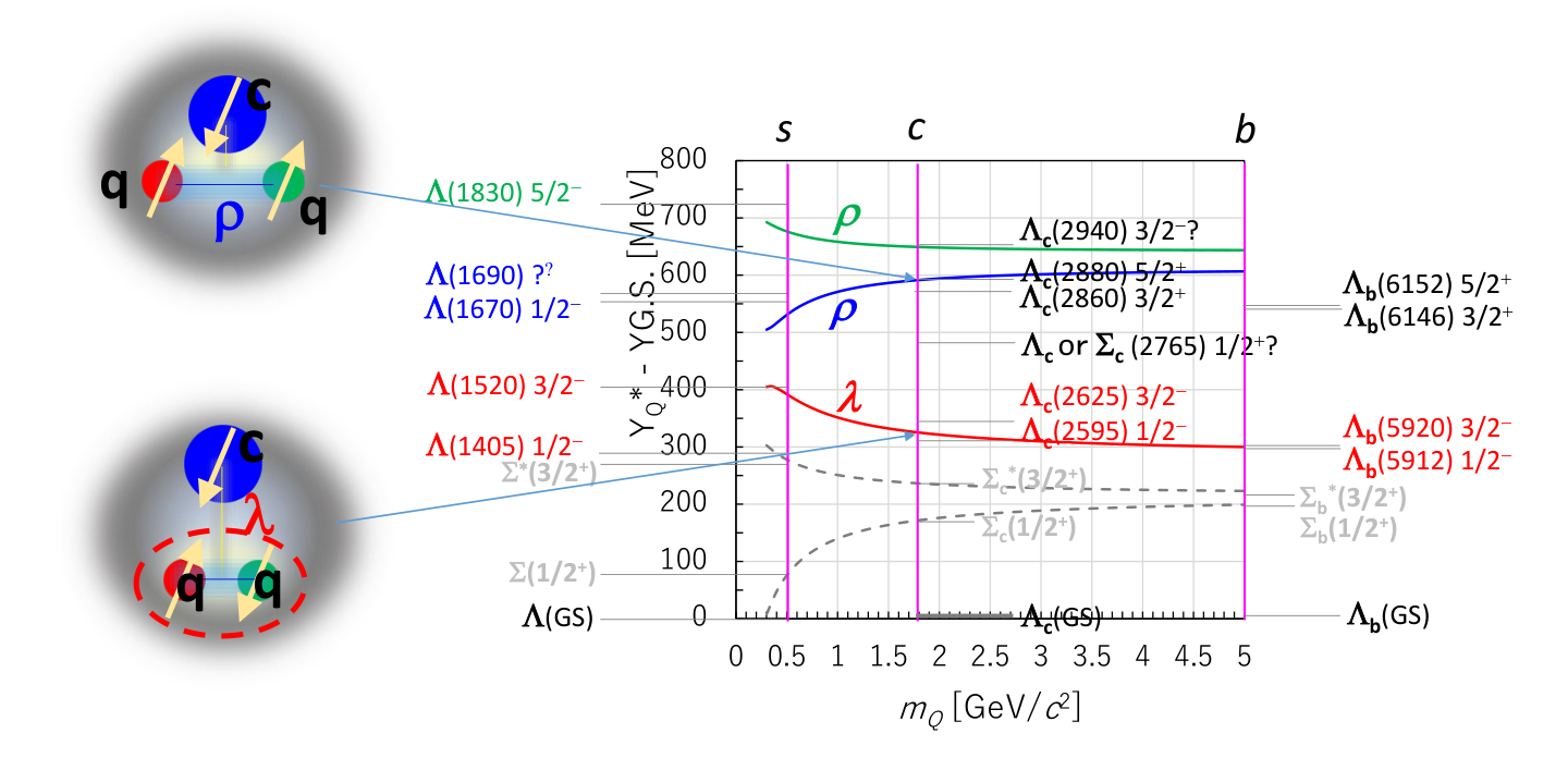

3.8.3 Baryon with a single heavy quark and two-strange quarks
Now let us turn to the systems of , baryons. In Fig. 114, we draw 5 lines for excited S- and P-states, connecting the states with having the same spatial (parity) and spin configuration but different masses (flavors). Excitation energies for , , , and reported by the Particle Data Group (PDG) [1233] are overlaid for reference. Most of their quantum numbers have not been determined. The behaviors of 5 lines are similar to the cases in the system. The internal configuration of the system is constraint due that the pair must be flavor-symmetric. In fact, the S-wave systems with the spin-singlet is forbidden, however their masses can be numerically evaluated. It should be noted that the excitation energies shown in Fig. 114 are relative to the forbidden states (indicated as in the figure) as one can recognize the similarity of to . From Fig. 114, we observe unique features. The excitation energy of the mode is lower than that of the mode in . The state is a candidate of the -mode excited states. If so, its decay into or is expected to be dominant. One of the pair in the -mode state, where is or , is expected to be the so-called ”good” diquark, the spin singlet state, and thus the state reflects the diquark correlation. Several states are observed but little of spin-parities and decay branching ratios are known. At K10, we will populate the states in the reactions, as shown in Fig. 98. We will determine the excitation modes and properties of the excited states by measuring their decay branching ratios and angular distributions.
is made of only quarks. The level structure of baryons becomes much simpler due to flavor symmetry. The and modes are degenerated (the point of the upper circle at ), and forbidden modes at due to the Pauli exclusion principle (crosses at . These observations are not yet established experimentally that can be primarily studied in the K10 project. In addition, there is further unique features in the baryons as we discuss below.
The systems with no , quarks that we have discussed so far are considered very different from the protons and neutrons, where pion clouds surround the nucleon forming the tail of the structure. Hence we have a picture for the nucleon, the quark core and the pion cloud around it. The pion of light mass is the necessity of spontaneous symmetry breaking of chiral symmetry and leads to various model independent relations as the low energy theorems. The pion also gives the most important component of the nuclear force at long distances. In spite of these good features, the pion may complicate the structure of the nucleon and makes it difficult to establish a unified description including its resonances. Moreover, the light pions are easily emitted from the resonances, that makes theoretical analysis involved.
In the standard quark model where the pion cloud is not taken into account, baryons are and their resonances are described as single particle excitations of the constituent quarks. In this word, the quark model explains properties of many low lying hadrons qualitatively with various flavors including heavy quarks. It also describes the short range part of the nuclear force which has been supported by the recent lattice calculations. A very opposite description of the nucleon emerges when maximally utilizing the pion cloud. This is the skyrmion for the nucleon. In this picture the nucleon excitations emerge as collective motion of the pionic soliton. The model is good at describing the phenomena where the pion is involved. The nucleons or in general hadrons containing light quarks share both features quark dynamics and pion dynamics in some way or another.
The two models reflect important aspects of QCD, but their advantages are somewhat different. In some cases they make very different predictions. Under such situation, we propose to explore the study of baryons removing pion clouds, “pionless spectroscopy”. This should be useful to unveil the genuine role of the constituent quarks, and in turn that of the pions. Our eventual goal is then to establish an effective method keeping its applicability to explain and predicts various hadron phenomena.
3.8.4 High-energy hyperon and proton scattering
At the K10 beam line, a huge amount of free ground-state hyperons are expected to be produced such as , , , and . These hyperons are rather stable or long-lived since they can decay only with the weak interaction. Of primary importance for the interaction between a hyperon and the nucleon would be the -wave (and -wave) low-energy scattering. However, scattering on the nucleon at higher energies would provide information on the size of hyperons, and interaction mechanism (what the exchange particle is). We have estimated the expected momentum distributions for the free hyperons produced at the K10 beam line by using the JAM code [1279]. Fig. 115 shows the momentum distributions for the produced hyperons. Among the ground-state hyperons, it is difficult to use ’s since they decay promptly after production not with the weak interaction but with the electromagnetic interaction. A missing-mass technique enables us to obtain the momentum-tagged hyperons. The momentum of the produced shows a bump at 4.5 GeV/c, covering a wide range from 2 to 8 GeV/. The momentum distributions are rather flat from the minimum (1 GeV) to the maximum (10 GeV/) for and . The two peaks at the minimum and maximum momenta come from the backward and forward direct production in the , respectively. Almost all the ’s and ’s have the momenta below 4 GeV/ but the momenta reach 10 GeV. We can study the hyperon and nucleon collisions at CM energies GeV and up to GeV where the reaction cross section are not affected by appearance of baryon resonances.
The total cross section provides an input to the size of baryons. In a classical situation, one obtains the total cross section of for the two balls with radii of and . Given the transverse position of the first ball, the second one must be within an area of to make the two collide. The total cross section in the two-baryon collision must include information on the sum of their radii. Figure 116 shows the total cross section as a function of the CM energy . It shows a prominent enhancement in each of , , and collisions near the threshold owing to strong attraction in the corresponding -wave channel. It should be noted that an enhancement in the and collisions is larger than that in because of the existence of a or bound state, or the deuteron. After that shows a complicated structure below a few GeV having several enhancements corresponding to the appearance of baryon resonances.
At high energies, increases as the square of a logarithm (relativistic rise of ):
| (48) |
With greater energy, a baryon can excite the other baryon and produce one or several mesons on it from ever greater distances. Since the radius of interaction is thus growing, so is the total cross section. In the intermediate energies from a few to several tens of GeV, is almost constant, mb, independently of the kind of baryons, indicating a core of a baryon measures fm in radius. Since we do not expect a pion cloud in , a smaller value than mb would be obtained for in the collision. The relativistic rise of would be also highly suppressed for , resulting is constant in a wide energy region.
Another important feature of the hyperon and proton collision would appear in diffractive elastic scattering (elastic scattering at small angles) which is directly connected to the longstanding problem of QCD at large distances. Especially, and scatterings are of particular interest. In these scatterings, a single pion exchange is forbidden owing to the isospin conservation between the initial and final isoscalar ’s or ’s. Owing to the - coupling as well as - mixing coming from the isospin symmetry breaking, scattering takes place more likely than scattering. The - coupling enables a sequential transition, and a pion exchange takes place in each step. It is difficult to consider a similar sequential transition for scattering. The scattering also takes place with a single pion exchange at a few percent level isospin breaking. It is also difficult to consider a similar situation for scattering. In elastic scattering, only , and exchanges are allowed in the first order. The systematic studies of high-energy scatterings allow us to study the reaction mechanisms of diffractive process (what the exchange particle is).
3.8.5 Differential cross section as a function of for production
The differential cross section for charmed-baryon production, corresponding to the transition form factor from the nucleon to the charmed baryon, includes information on the internal structure of the charmed baryon. The can be determined from the events where the mesons are emitted at finite angles. Figure 117 shows the angular distribution of emission and acceptance of the -produced events as a function of the emission angle in the CM frame ( and ) together with those as a function of . Here, the differential cross section was assumed to take a form
| (49) |
with a slope parameter . Acceptance of the -produced events detected with the E50 spectrometer was found to be 80% almost independently of the emission angle or . Figure 118 shows the distributions for the generated and accepted events (the number of accepted events is ). A value of was obtained for the slope parameter by fitting an function (49) to the distribution for the accepted events. To determine the slope parameter correctly, we need acceptance correction as a function of but the fitting result of indicates that we can extract the slope parameter with a statistical error of 3.6%.


3.8.6 Background reduction for production
The estimated cross section of production is 10-4 smaller in the reaction than that of hyperon () production (10–100 b for ). Thus, it is necessary to reduce the background contribution significantly for observing ’s and determine their masses and widths. To optimize the background reduction, we investigate three kinds of background processes: 1) strangeness production, 2) wrong particle identification, and 3) production associated without the of interest. Although strangeness production is the main contributor to the background, the corresponding events are effectively reduced by using a tagging method. Figure 119 shows the correlation plots between and where the value corresponds to the excitation energy of (). A reduction factor of 2 was obtained by selecting the events that satisfied GeV ( mass) and MeV. Although the reduction factor of tagging is quite high, we have still a sizable background contribution. Other possible methods for further reducing the background contribution are to use the opening angle in the CM frame between and from , and to use the kinematic condition corresponding to the -channel in the reaction. Additional reduction factor of 15 can be achieved from these although survival ratio of the events of interest is 0.54. The final background level is expected to 5 counts/MeV in average at masses ranging from 2.2 to 3.4 GeV.
Wrong particle identification also deteriorates the background level. We also estimated its effect taking into account the limited performance of the PID detector, and obtained a similar level of 6 counts/MeV to that of strangeness production. The -produced events associated without the of interest. were also investigated by using the Geant4 simulation with JAM. The contribution was minor compared with the strangeness production and the wrong particle identification events. Finally, the the average background level was found to be 11 counts/MeV at masses ranging from 2.2 to 3.4 GeV. It is difficult to estimate the systematic uncertainty of the background level since we do not have any experimental data currently. We just compared the estimated background levels obtained from the JAM [1279] and PYTHIA [1286] codes, and considered the systematic uncertainty was a factor of 2. The sensitivity of the production cross section was found to be 0.1–0.2 nb.

3.8.7 Possible background reduction for observing highly-excited s


The background contribution gradually increases with increase of the missing mass, and the peaks are difficult to be observed in the mass region above 2.2 GeV. It is crucial to make the S/N ratio higher for observing highly-excited ’s. Selecting the events that contain the daughter particles from ’s is a possible way to get the higher S/N ratio. From now on, we focus on the and decay channels since their branching ratios are expected to be large. It should be noted that the produced ’s can decay into not only the channels described above but also other channels in the simulation depending on the JAM parameters. Figure 120(a) shows the missing-mass spectrum for the background events generated by JAM. Three peaks are clearly observed at masses of 0.94, 1.02, and 1.19 GeV. The 0.94-GeV (1.19-GeV) peak corresponds to the events that the proton () is missing. The 1.02-GeV peak is made by the proton and () from the decay. The generated events in JAM include ’s from , which decay into and . Since decays into , the and peaks are generated. It should be noted that the final-state can be identified as because of its broad width. A detailed analysis of the production and decay vertices is expected to remove these background processes. Figure 129(b) shows the missing-mass spectrum for the background events. A peak corresponding to can be observed with a small yield. Figures 120(c) and (d) show the correlation plots between the and the missing masses, and between and the , respectively. To remove the background contribution to the -produced events with the decay, we select the events that the missing mass is consistent with the mass. Similarly, the events can be selected with background suppression in the high-mass region by applying the condition that the missing mass is consistent with the mass. Figure 121 shows the missing-mass spectra for the background events after selecting the events that contain from the decay or from , showing a reduction factor of more than 200 in the high-mass region. A significant improvement of the S/N ratios are expected only if the branching ratios are or larger for the and decays.
3.8.8 Performance of the spectrometer for observing s
The performance of the E50 spectrometer for the -produced events has been estimated by a Monte Carlo simulation based on Geant4. In this sub-subsection, described are the acceptance of the -produced events, the experimental -mass resolution, and their yields.
(a) Acceptance of the -produced events
The -produced events are selected by using the missing mass. It is necessary to detect the final-state () particles from emitted at forward angles. Estimated is the acceptance for the -produced events, or a fraction of the events that all the () particles are detected. Fig. 122(left) shows the detector acceptance for the -produced events (the ground state) as a function of the incident kaon momentum. The detector acceptance for the -produced events are found to be – and in the and reactions, respectively. Here, the angular distribution of production is assumed to be isotropic in the -CM frame. It should be noted that the acceptance includes the effects of final-state and decays in flight. The acceptance gradually increases with increase of the incident kaon momentum in the reaction, while it is almost independent of the incident momentum below 10 GeV/ in . Figure 122(right) shows the acceptance for the -produced events below the excitation energy of 1 GeV at the incident kaon momentum of 10 GeV/. The angular distribution of production is also assumed to be isotropic in the -CM frame. The acceptance becomes higher with increase of the excitation energy both in the two reactions. This is because () are likely to be emitted at forward angles where the E50 spectrometer has high acceptance in case of producing high-mass ’s.


The daughter particles from the decays are covered by the internal detectors. The horizontally-emitted particles finally comes to the detectors in front of the yoke, and the vertically-emitted to those on the pole pieces. Owing to these internal detectors, a wide coverage is obtained for the polar angles of emission (opposite to the direction of emission) in the rest frame from the two-body decay of (). The acceptance of the events detecting () is found to be 95% (90%) in the two-body (three-body ) decay. It should be noted that the acceptance described above does not include the effects of final-state and decays in flight. The effects of the in-flight decay of ’s deteriorate the acceptance by 10%. Figure 123 shows the acceptance of detecting the two-body decay as a function of the emission angle in the rest frame. Here, -axis is defined to be opposite to the direction of the composite system produced in association with . The daughter from the decay is emitted at forward angles in the laboratory frame, and the acceptance is high for detecting the decay. Some acceptance drop is observed at the emission angle of . In this case, the associated ’s are emitted at backward angles, and some of them are out of the angular coverage of the E50 spectrometer. Owing to high acceptance of the events with identifying the decay, we can obtain the decay angular distribution, and determine the corresponding branching ratio.
(b) -mass resolution


The resolution is estimated for the mass, which is calculated as the missing mass in the reaction, or the missing mass in the reaction. Here, the momentum resolutions are assumed as same as those in the planned E50 experiment for the incident kaon momentum, and for each of the final-state and particles detected with the E50 spectrometer in the , and reactions, respectively. The incident momentum resolution assumed is a fixed value of (). The momentum resolution assumed is () for 5-GeV/ particles detected with the E50 spectrometer, and is given by at a certain momentum . The 2-MeV () straggling is incorporated for the energy loss in the target material, which corresponds to the 4-g/cm2 thickness of the hydrogen target. The target thickness should be decided in the actual experiment considering the balance between the mass resolution and yield for ’s.
Figure 124 shows the resolution () of the (ground state) mass as a function of the incident kaon momentum in the (left) and (right) reactions. The momentum becomes higher for each of the final-state () with increase of the incident momentum, deteriorating the resolution of the mass as well as that of the momentum of each final-state particle. Figure 125 shows the resolution () of the mass as a function of the excitation energy at the incident kaon momentum of 10 GeV/. The mass resolution becomes higher with increase of the excitation energy since production of high-mass makes the momentum lower for each final-state particle out of (). The mass resolution is found to be 2.5–4.5 MeV () depending on the incident kaon momentum and excitation energy. The high mass-resolution and narrow width of ( is expected from several MeV to several tens of MeV for ’s) enable us to observe s separably. Additionally, the width is expected to be measured directly since the mass resolution is comparable or smaller than the width.
(c) Yield of the -produced events
We estimate the expected yields of the -produced events detected with the E50 spectrometer at the K10 beam line. The existing data show that the total cross section ranges from 2.0 to 3.5 b at incident kaon momenta ranging from 7 to 10 GeV/ for inclusive production in the reaction: b at 4.2 GeV [1287, 1288], b at 6.5 GeV [1289], b at 8.25 GeV [1290], b at 10 GeV [1291], and b at 11 GeV [1292]. The reaction dominates in inclusive production at incident kaon momentum below 10 GeV/. Thus, we simply assume the cross sections are 2.0 and 3.5 b for the reaction at incident kaon momenta of 7 and 10 GeV, respectively. Since the total cross section increases rather linearly with increase of the incident kaon momentum, the total cross section is given by interpolating the 7- and 10-GeV cross sections to give a cross section at a certain incident momentum. Among the inclusive -produced events at 4.2 GeV/ in Ref. [1288], the numbers of events containing and in the final state are 39 and 1, respectively. We assume that the total cross section of the reaction is 1/40 that of at a fixed incident kaon momentum between 7 and 10 GeV/. This assumption might not be realistic since a branching ratio of 50% for the decay is ignored here, and since the reaction is suppressed owing to the limited phase space at 4.2 GeV/. We suppose these two effects are canceled out at incident kaon momenta of 7–10 GeV/. Additionally, the production cross section of an is assumed to be the same as that of depending on the reaction and incident kaon momentum.
| Reaction | ||
|---|---|---|
| Cross section | 0.06 b | 2.50 b |
| Branching ratio | 0.67 () | 0.35 () |
| Beam intensity | /spill (2-s duration in a 5.2-s cycle) | |
| Target thickness | 4.0 g/cm2 (57-cm-thick hydrogen) | |
| Acceptance ( production) | 0.48 | 0.23 |
| Tracking efficiency | 0.90 (each particle) | |
| Particle identification | 0.97 (each particle) | |
| Data acquisition efficiency | 0.99 (Streaming DAQ) | |
| Total efficiency | 0.66 (three-track events) | |
| yield in a day | ||
| yield in a 100-day beam time | ||
| Acceptance ( decay) | 0.86 |
|---|---|
| (including in-flight decay of ) | |
| Decay branching ratio ( decay) | 0.30 |
| Total efficiency for detecting | 0.75 |
| yield in a 100-day beam time | |
| (each bin out of 20 angle bins) |
The expected yield of the -produced events is estimated in the following assumptions: the cross section of production is 0.06 b and 2.50 b at the incident kaon momentum of 8 GeV/ in the and reactions, respectively, the tracking efficiency is 0.90 for each particle; the particle-identification efficiency is 0.97 for each final-state particle from ; DAQ efficiency is 0.99; and the total efficiency is for three-track events. The acceptance of the events for each reaction includes in-flight decay of the final-state particles to be detected (both and ). Table 20 summarizes the factors assumed for the yield estimation of production. The expected yields of -produced events are and a day in the and reactions, respectively. To obtain several of the -produced events, we need a 100-day beam time. In analysis of the decay angular distribution of , the -produced events may be combined for the and reactions, and more than -produced events are available in a 100-day beam time. Suppose the branching ratio is 0.3 for the two-body decay, the expected yield is several thousands for each bin of emission angles divided into 20. Additional factors are listed in Table 21 to get the expected yields in the decay angular distribution.
3.8.9 Expected -mass spectrum
(a) Spectrum without the background contribution
At first, we show the expected -mass spectrum without any background processes. The ’s considered are summarized in Table 22, which are taken from the Review of Particle Physics [1233]. Additionally, we incorporate a Rope-like resonance with the parameters described in Table 22.
| Mass [MeV] | Width [MeV] | |
|---|---|---|
| 2470 | 72 | |
| 2380 | 26 | |
| 2250 | 55 | |
| 2160 | 100 | |
| 2012 | 6.4 | |
| 1672 | — |
Figure 126 shows the expected -mass spectrum without any background processes at the incident kaon momentum of 8 GeV. Here, the mass is given by the missing mass, and the number of produced ’s is fixed at for each corresponding to a 100-day beam time. Peaks are separably observed for narrow ’s with widths narrower than 30 MeV, and those are clearly distinguished from others even for rather wide ones. It should be noted that all the experimental resolutions are included: momentum resolution, angular resolution, and straggling of the energy loss in the target material.

Since the number of events is in each peak, the precision of the mass determination in this spectrum is better than 1 MeV depending on the width of the corresponding . To get accuracy of the mass determination, the absolute momentum scale in the spectrometer is required to be calibrated carefully. We can use various peaks corresponding to hyperons and other baryons in similar mass spectra. Thus, the accuracy expected is also better than 1 MeV after the calibration.
It is difficult to accurately determine the width of an . The observed peak must be modified by the experimental mass resolution of 2.5–4.5 MeV (). The peak may be different in shape from the Breit-Wigner function owing to the overlap with other peaks and background contributions, and interference with other processes. The accuracy of the width determination expected is better than 1 MeV for an isolated Breit-Wigner peak with a width of 10 MeV. We expect the accuracy of the width determination is better than a few MeV for high-mass ’s, which are overlapped with other contributions.
(b) Background contribution
It is difficult to estimate the background contribution correctly in the -mass spectrum obtained from the reaction for several-GeV/ incident kaons. Available experimental data are quite limited in this momentum range, and we cannot estimate inclusive cross sections or multiplicities of generated particles even if we find some exclusive cross sections in a particular reaction. Thus, we use a hadron-reaction generating code called JAM (version 1.90597) [1279] for the background estimation as usual. JAM includes many elementary reaction processes at wide CM energies, covering the resonance region ( GeV), the string region ( GeV), and the perturbative-QCD (pQCD) region ( GeV).
| Beam | Ratio [%] | Ratio [%] | |||||
|---|---|---|---|---|---|---|---|
| [GeV/] | [mb] | [b] | [b] | [b] | [b] | ||
| 7.0 | 25.6 | 463 | 1.80 | 2.00 | 0.050 | 0.43 | 2.8 |
| 8.0 | 23.6 | 503 | 2.46 | 2.50 | 0.063 | 0.50 | 2.6 |
| 9.0 | 23.2 | 548 | 3.16 | 3.00 | 0.075 | 0.55 | 2.4 |
| 10.0 | 22.6 | 585 | 4.22 | 3.50 | 0.088 | 0.60 | 2.0 |
Of interest in the proposed experiment is the string region where hadrons are generated mainly in the string-string scattering processes. The hadronization process is described in the Lund string model [1293], which is also adopted in another hadron-reaction generating code called PYTHIA [1286]. Adjusted in JAM to reproduce the existing experimental data are the conditions of the string-string scattering and hadronization processes: no string-string scattering before hadronization, no color-flow during the string generation, and the production ratios of the generated hadron resonances. Those conditions and hadron resonances considered are different from those in PYTHIA. Here, we do not use PYTHIA but JAM since we have found JAM reproduces the experimental data better than PYTHIA at incident momenta of several GeV/1616 16 We have investigated both the codes, and compared with the experimental data for the background studies in the E50 experiment for spectroscopy of charmed baryons [1246]..
Table 23 shows the cross sections for the background contributions estimated by JAM together with those assumed for the signal -produced processes. We investigate and production as the background contribution. The cross section for the -produced events is found to be two-order smaller than that for -produced events. Thus, the -mass spectrum obtained in the reaction is expected to have low background as compared with that in the . Additionally, some of candidates reconstructed from can be so that the -mass spectrum includes the - and -produced events. It is necessary to detect not but for reducing the background contribution in the -mass spectrum. We can obtain the -mass spectrum with high S/N ratio from the missing mass which gives only an system.
(c) Smaller -production cross sections
Even if the cross section is smaller by a factor of 1/3, we can still recognize the , , , and peaks. Figures 127 and 128 show the expected -mass spectra including the background contribution at the incident kaon momentum of 8 GeV by reducing -production cross sections by a factor of 1/1, 1/3, 1/10 and 1/30. If the cross section is smaller by 1/10 than that in the original assumption (63 nb), it is difficult to identify peaks except for the ground-state and first-excited . In this case, additional background reduction is required for finding an with a broad width.


(d) Possible background reduction

We plan to determine the mass spectrum of ’s originally without using any information on their decay. Selecting the events that contain the daughter particles from ’s is a possible way to get the higher S/N ratio. From now on, we focus on the decay channel since its branching ratio is expected to be large. It should be noted that the produced ’s can decay into not only the channel described above but also other channels in the simulation depending on the JAM parameters. Figure 129(a) shows the missing-mass spectrum for the background events generated by JAM. In Fig. 129(a), peaks corresponding to , , and are observed. The generated events in JAM include those from , showing the and peaks. The events forming the peak come mainly from the decay of the ground-state which is included in JAM. It also comes from the reaction followed by the and decays. Since the width of is rather broad, and in the final-state of this reaction sequence can be identified as . Detailed analysis of the production and decay vertices is expected to remove this background process. Figure 129(b) shows the missing-mass spectrum for the background events. A peak corresponding to can be observed clearly. Above this peak, a huge amount of the continuum background events are observed which prevent us from observing highly-excited ’s. Figure 129(c) shows the correlation plot between the the and the missing masses. By selecting the events that the missing masses are consistent with the mass, we can remove huge background concentrated as shown in Fig, 129(c) at a missing mass of GeV and a missing mass of GeV. Figure 129(d) shows the missing-mass spectrum for the background events after selecting the events that the missing masses are consistent with the mass. As compared with Fig. 129(b), the background level has been reduced by a factor of /10 or 1/100. To get a significantly improved S/N ratio, the branching ratio must be or higher for the decay.
Selecting the events containing as a daughter particle from the decay is effective at background reduction in the -mass spectrum if the branching ratio is for the decay. As shown in Figs. 130 and 131, the S/N ratio is improved by a factor of 1/10 for the high-mass ’s so that we can recognize ’s with a broad width even when the cross section is smaller than that originally assumed. We can also find the or the Roper-like state having a broad width of 100 MeV even if the cross section is smaller by 1/10 than that in the original assumption. Since is a rather stable particle, we can recognize its flight path before decaying. Thus, detailed analysis of the production and decay vertices of an would help us to get the further higher S/N ratio.


(e) Different incident kaon momenta

Thus far, shown are only the expected -mass spectra at the incident kaon momentum of 8 GeV/. We also estimate those at several different incident kaon momenta. Figure 132 shows the expected -mass spectra at incident kaon momenta of 7, 8, 9, and 10 GeV. The excitation-energy range covered in the measurement becomes wider with increase of the incident kaon momentum, and high-mass ’s are likely to be observed up to the excitation energy of 1.5 GeV at the highest incident kaon momentum of 10 GeV/. Within the excitation-energy coverage, all the peaks corresponding to ’s are clearly observed with high S/N ratios. It is important to measure the -mass spectra at different incident kaon momenta. A fake structure may appear caused by some kinematic effects since the measured spectrum reflects the appearance of a resonance in other system of the final-state particles than that corresponding to ’s. This kind of kinematic effects are observed in a different shape at a different incident kaon momentum. The mass spectra with several incident momenta enable us to identify fake structures coming from the kinematic effects. The mass spectra with different incident momenta are also useful for determination of the the widths. The optimum incident kaon momentum is different for different excitation energies since the sensitivity of the width determination highly depends on the background level and background shape.
3.8.10 Spin-parity determination of s
The spin-parity assignment of a produced provides crucial insight into the internal quark motion. Here, we discuss possible ways to determine the spin-parity of . First, we determine the spin of from the angular distribution of . Since the spin of is 1/2 and that of is 0, the distribution of () emission in the rest frame of is expressed using the spin-density matrix (SDM) of with a spin of as
| (50) |
Here, is the emission angle of the daughter particle ( or ) with respect to the axis in the rest frame of , and denotes the diagonal elements of SDM. It should be noted that . We have several choices for the -axis. Suppose -axis is defined to be opposite to the direction of the composite system produced together with . In this case, is equivalent to the helicity of , and non-uniform helicity distribution enables us to determine the spin of . However, we obtain the uniform angular distribution independently of the spin of when the helicity distribution is uniform. Taking into account the reaction followed by the decay alternatively, we can define the axis is the normal vector of the -production plane containing the initial - and final -momentum vectors. The must be polarized and is also expected to be polarized in some fraction with respect to this axis.

We show here how to obtain the angular distribution of emission (decay angular distribution) of an in the two-body decay. The branching ratio assumed is 0.3 for this decay channel. In principle, the -produced events are identified by using the missing mass. The decay angular distribution can be given additionally detecting the daughter from the decay. Here, we take an example for the decay angular distribution for as an . We select the events that the and missing masses are close to the and masses, respectively. The selected region is indicated in Fig. 133(c). Figure 133(b) shows the missing-mass spectrum for the background events after selecting the events near the mass in the missing-mass spectrum, and Figure 133(d) for the -produced events. Let us look at the missing-mass spectrum as shown in Fig. 133 (b) for the background contribution and in Fig. 133 (d) for production. The background contribution is well suppressed and distributed in a wider range as compared with production. Thus, a side-band subtraction method can be used to extract the -produced events for deduction of the decay angular distribution. The decay angular distribution can be obtained similarly to for the other ’s.
We estimate the decay angular distribution in the rest frame of the produced . Here, we take the -axis along the opposite direction to the momentum of the composite system produced together with . Figure 134 shows the acceptance-corrected decay angular distribution. The isotropic decay angular distributions are obtained according to isotropic event generation of the decay in the simulation. The azimuthal-angle asymmetry is simply ignored here, the effect of which is canceled out in the polar angle distribution. The can be determined by fitting a function expressed by Eq. (50) to the observed angular distribution. In Fig. 134, the functions corresponding to the isotropic generation (uniform sub-population for a certain ) and the case with for are plotted. When the angular distribution shows some structure, we may identify and determine ’s with an error of 1%. We can perform more detailed analysis for determining the spin for the of interest by combining other information such as the branching ratio.

When we observe an isolated state with a certain spin-parity in the reaction followed by and decays, we can determine the spin-parity of from the angular correlation between and . Figure 135 shows the typical angular correlations for the transitions for certain spin-parities of and , and angular momenta carried by meson emissions. Here, we have calculated the and angular correlations for the sequential decay of using the density matrix (statistical tensor) formalism [1294]. It should be noted that the spin-parity of can be determined in its decay into the ground-state with a spin-parity of , . The angular correlation is isotropic (uniform) when the spin of is 1/2. In this case, the parity of is determined by using the polarization transfer from to similarly to the parity determination of by the CLAS collaboration [1295]. When the spin-parity of is (), the decay takes place in the () wave. The polarization direction of , which can be obtained from the decay asymmetry of , is parallel to that of in the -wave case. On the hand, the polarization direction is expressed by where denotes the emission angle with respect to the polarization direction of .
It is important to find a sequential decay for with a known spin-parity for the spin-parity determination of . Figure 137 shows possible decays from to . The solid arrows indicate the observed decays listed in Review of Particle Physics [1233]. The ’s are expected to decay directly into the ground-state by emitting . Even if this direct decay is not observed, we can expect the decay into a low-lying state of which spin-parity is known, for example. On the other hand, it is uncertain to find an isolated state decaying into . Figure 137 shows possible decays from to . There are several predicted highly-excited s, which can play a role as a doorway to production. These ’s decay into or by emitting , and they must also decay into by emitting . Since the statistical tensor formalism can treat a mixed state for each of intermediate states and meson emissions, we can also estimate the interference effects between several states and those with background contributions.
We also expect to determine the parities from the decay widths for some ’s. Let us consider an with a spin of 1/2 decaying into . The angular momentum carried by emission is 0 and 1 for the negative and positive parities of the , respectively. The decay width is proportional to where denotes the relative momentum between the daughter particles. Thus the branching ratio of with respect to would be useful for the parity determination.
References
- [657] S. Nagamiya In Nucl. Phys. A774, 2006, pp. 895 DOI: 10.1016/j.nuclphysa.2006.06.160
- [658] Shoji Nagamiya In Prog. Theor. Exp. Phys. 2012, 2012, pp. 02B001 DOI: 10.1093/ptep/pts025
- [659] B.. Abbott In Phys. Rev. Lett. 119, 2017, pp. 161101 DOI: 10.1103/PhysRevLett.119.161101
- [660] Andrzej. Buras, Dario Buttazzo, Jennifer Girrbach-Noe and Robert Knegjens In J. High Energy Phys., 2015, pp. 033 DOI: 10.1007/JHEP11(2015)033
- [661] Keizo Agari In Prog. Theor. Exp. Phys. 2012, 2012, pp. 02B008 DOI: 10.1093/ptep/pts034
- [662] Taku Yamanaka In Prog. Theor. Exp. Phys. 2012, 2012, pp. 02B006 DOI: 10.1093/ptep/pts057
- [663] Keizo Agari In Prog. Theor. Exp. Phys. 2012, 2012, pp. 02B009 DOI: 10.1093/ptep/pts038
- [664] Hiroyuki Fujioka, 2017 arXiv:1706.07916 [nucl-ex]
- [665] Hadron’, 2019 arXiv:1906.02357 [nucl-ex]
- [666] Tadashi Koseki In Prog. Theor. Exp. Phys. 2012, 2012, pp. 02B004 DOI: 10.1093/ptep/pts071
- [667] M. Moritsu In Phys. Rev. C90, 2014, pp. 035205 DOI: 10.1103/PhysRevC.90.035205
- [668] R. Honda In Phys. Rev. C96, 2017, pp. 014005 DOI: 10.1103/PhysRevC.96.014005
- [669] Toru Harada, Ryotaro Honda and Yoshiharu Hirabayashi In Phys. Rev. C 97, 2018, pp. 024601 DOI: 10.1103/PhysRevC.97.024601
- [670] Y. Ichikawa In Prog. Theor. Exp. Phys. 2015, 2015, pp. 021D01 DOI: 10.1093/ptep/ptv002
- [671] T.. Yamamoto In Phys. Rev. Lett. 115, 2015, pp. 222501 DOI: 10.1103/PhysRevLett.115.222501
- [672] S.. Yang In Phys. Rev. Lett. 120, 2018, pp. 132505 DOI: 10.1103/PhysRevLett.120.132505
- [673] T. Yamaga In Phys. Rev. C 102, 2020, pp. 044002 DOI: 10.1103/PhysRevC.102.044002
- [674] T. Nagae In AIP Conf. Proc. 2130, 2019, pp. 020015 DOI: 10.1063/1.5118383
- [675] S. Kawasaki In JPS Conf. Proc. 26, 2019, pp. 022009 DOI: 10.7566/JPSCP.26.022009
- [676] H. Ekawa In Prog. Theor. Exp. Phys. 2019, 2019, pp. 021D02 DOI: 10.1093/ptep/pty149
- [677] S.. Hayakawa In Phys. Rev. Lett. 126, 2021, pp. 062501 DOI: 10.1103/PhysRevLett.126.062501
- [678] M. Yoshimoto In Prog. Theor. Exp. Phys. 2021, 2021, pp. 073D02 DOI: 10.1093/ptep/ptab073
- [679] K. Miwa, 2021 arXiv:2104.13608 [nucl-ex]
- [680] J.. Ahn In Phys. Rev. Lett. 126, 2021, pp. 121801 DOI: 10.1103/PhysRevLett.126.121801
- [681] H. Ohnishi, F. Sakuma and T. Takahashi In Prog. Part. Nucl. Phys. 113, 2020, pp. 103773 DOI: 10.1016/j.ppnp.2020.103773
- [682] Y. Ichikawa In Prog. Theor. Exp. Phys. 2020, 2020, pp. 123D01 DOI: 10.1093/ptep/ptaa139
- [683] H. Sugimura In Phys. Lett. B729, 2014, pp. 39 DOI: 10.1016/j.physletb.2013.12.062
- [684] K. Shirotori In Phys. Rev. Lett. 109, 2012, pp. 132002 DOI: 10.1103/PhysRevLett.109.132002
- [685] Yudai Ichikawa In Prog. Theor. Exp. Phys. 2014, 2014, pp. 101D03 DOI: 10.1093/ptep/ptu128
- [686] T. Hashimoto In Prog. Theor. Exp. Phys. 2015, 2015, pp. 061D01 DOI: 10.1093/ptep/ptv076
- [687] Y. Sada In Prog. Theor. Exp. Phys. 2016, 2016, pp. 051D01 DOI: 10.1093/ptep/ptw040
- [688] S. Ajimura In Phys. Lett. B789, 2019, pp. 620 DOI: 10.1016/j.physletb.2018.12.058
- [689] H. Asano In AIP Conf. Proc. 2130, 2019, pp. 040018 DOI: 10.1063/1.5118415
- [690] S. Okada In Prog. Theor. Exp. Phys. 2016, 2016, pp. 091D01 DOI: 10.1093/ptep/ptw130
- [691] T. Hashimoto In JPS Conf. Proc. 26, 2019, pp. 023013 DOI: 10.7566/JPSCP.26.023013
- [692] J.. Ahn In Prog. Theor. Exp. Phys. 2017, 2017, pp. 021C01 DOI: 10.1093/ptep/ptx001
- [693] J.. Ahn In Phys. Rev. Lett. 122, 2019, pp. 021802 DOI: 10.1103/PhysRevLett.122.021802
- [694] N. Shimizu In Phys. Rev. D102, 2020, pp. 051103(R) DOI: 10.1103/PhysRevD.102.051103
- [695] H. Ito, 2021 arXiv:2107.03583 [hep-ex]
- [696] H Takahashi In J. Radioanal. Nucl. Chem. 305, 2015, pp. 803 DOI: 10.1007/s10967-015-3940-9
- [697] Hiroaki Watanabe In JPS Conf. Proc. 28, 2020, pp. 041004 DOI: 10.7566/JPSCP.28.041004
- [698] Paul. Demorest et al. In Nature 467, 2010, pp. 1081 DOI: 10.1038/nature09466
- [699] John Antoniadis In Science 340, 2013, pp. 1233232 DOI: 10.1126/science.1233232
- [700] The CLAS Collaboration In Nature 560, 2018, pp. 617 DOI: 10.1038/s41586-018-0400-z
- [701] Bao-An Li, Bao-Jun Cai, Lie-Wen Chen and Jun Xu In Prog. in Part. and Nucl. Phys. 99, 2018, pp. 29 DOI: 10.1016/j.ppnp.2018.01.001
- [702] Megumi Naruki and Kotaro Shirotori In KEK/J-PARC-PAC 2014-4 2014-4, 2014
- [703] S.. Kim et al. In Prog. Theor. Exp. Phys. 2014, 2014, pp. 103D01 DOI: 10.1093/ptep/ptu131
- [704] Sang-In Shim, Atsushi Hosaka and Hyun-Chul Kim In Prog. Theor. Exp. Phys. 2020, 2020, pp. 053D01 DOI: 10.1093/ptep/ptaa049
- [705] Georges Aad In Phys. Lett. B 716, 2012, pp. 1 DOI: 10.1016/j.physletb.2012.08.020
- [706] Serguei Chatrchyan In Phys. Lett. B 716, 2012, pp. 30 DOI: 10.1016/j.physletb.2012.08.021
- [707] B. Abi In Phys. Rev. Lett. 126, 2021, pp. 141801 DOI: 10.1103/PhysRevLett.126.141801
- [708] Hideaki Hotchi In Prog. Theor. Exp. Phys. 2012, 2012, pp. 02B003 DOI: 10.1093/ptep/pts021
- [709] L. Tang In Phys. Rev. C 90, 2014, pp. 034320 DOI: 10.1103/PhysRevC.90.034320
- [710] A. Esser In Phys. Rev. Lett. 114, 2015, pp. 232501 DOI: 10.1103/PhysRevLett.114.232501
- [711] L. Adamczyk In Phys. Rev. Lett. 114, 2015, pp. 022301 DOI: 10.1103/PhysRevLett.114.022301
- [712] Shreyasi Acharya In Phys. Rev. C 99, 2019, pp. 024001 DOI: 10.1103/PhysRevC.99.024001
- [713] Kenji Morita, Takenori Furumoto and Akira Ohnishi In Phys. Rev. C 91, 2015, pp. 024916 DOI: 10.1103/PhysRevC.91.024916
- [714] Shreyasi Acharya In Phys. Lett. B 805, 2020, pp. 135419 DOI: 10.1016/j.physletb.2020.135419
- [715] J. Rowley, 2021 arXiv:2108.03134 [hep-ex]
- [716] Eduardo Cortina In J. High Energy Phys. 06, 2021, pp. 093 DOI: 10.1007/JHEP06(2021)093
- [717] Matthew Moulson In J. Phys. Conf. Ser. 1526, 2020, pp. 012028 DOI: 10.1088/1742-6596/1526/1/012028
- [718] M.. Miller In The Astrophysical Journal 887, 2019, pp. L24 DOI: 10.3847/2041-8213/ab50c5
- [719] B.. Abbott In Phys. Rev. Lett. 121, 2018, pp. 161101 DOI: 10.1103/PhysRevLett.121.161101
- [720] J.. Lattimer In Ann. Rev. Nucl. Part. Sci. 62, 2012, pp. 485 DOI: 10.1146/annurev-nucl-102711-095018
- [721] T. Hasegawa In Phys. Rev. C 53, 1996, pp. 1210 DOI: 10.1103/PhysRevC.53.1210
- [722] O Hashimoto and H Tamura In Prog. Part. Nucl. Phys. 57, 2006, pp. 564 DOI: 10.1016/j.ppnp.2005.07.001
- [723] Gal. A., E.. Hungerford and D.. Millener In Rev. Mod. Phys. 88, 2016, pp. 035004 DOI: 10.1103/RevModPhys.88.035004
- [724] I. Vidana et al. In Phys. Rev. C 61, 2000, pp. 025802 DOI: 10.1103/PhysRevC.61.025802
- [725] H.-J. Schulze and T. Rijken In Phys. Rev. C 84, 2011, pp. 035801 DOI: 10.1103/PhysRevC.84.035801
- [726] Haris Djapo, Bernd-Jochen Schaefer and Jochen Wambach In Phys. Rev. C 81, 2010, pp. 035803 DOI: 10.1103/PhysRevC.81.035803
- [727] H.. Cromartie In Nature Astronomy 4, 2020, pp. 72 DOI: 10.1038/s41550-019-0880-2
- [728] Robert. Wiringa, V… Stoks and R. Schiavilla In Phys. Rev. C 51, 1995, pp. 38 DOI: 10.1103/PhysRevC.51.38
- [729] Robert. Wiringa and Steven. Pieper In Phys. Rev. Lett. 89, 2002, pp. 182501 DOI: 10.1103/PhysRevLett.89.182501
- [730] J. Fujita and H. Miyazawa In Prog. Theor. Phys. 17, 1957, pp. 360 DOI: 10.1143/PTP.17.360
- [731] K. Sekiguchi In Phys. Rev. C 65, 2002, pp. 034003 DOI: 10.1103/PhysRevC.65.034003
- [732] A. Akmal, V.. Pandharipande and D.. Ravenhall In Phys. Rev. C 58, 1998, pp. 1804 DOI: 10.1103/PhysRevC.58.1804
- [733] B.. Pudliner, V.. Pandharipande, J. Carlson and Robert. Wiringa In Phys. Rev. Lett. 74, 1995, pp. 4396 DOI: 10.1103/PhysRevLett.74.4396
- [734] B.. Pudliner et al. In Phys. Rev. C 56, 1997, pp. 1720 DOI: 10.1103/PhysRevC.56.1720
- [735] J. Carlson et al. In Rev. Mod. Phys. 87, 2015, pp. 1067 DOI: 10.1103/RevModPhys.87.1067
- [736] M. Oertel, M. Hempel, T. Klähn and S. Typel In Rev. Mod. Phys. 89, 2017, pp. 015007 DOI: 10.1103/RevModPhys.89.015007
- [737] Kota Masuda, Tetsuo Hatsuda and Tatsuyuki Takatsuka In The Astrophysical Journal 764, 2013, pp. 12 DOI: 10.1088/0004-637x/764/1/12
- [738] Gordon Baym et al. In Rept. Prog. Phys. 81, 2018, pp. 056902 DOI: 10.1088/1361-6633/aaae14
- [739] V… Stoks, R… Klomp, C… Terheggen and J.. de Swart In Phys. Rev. C 49, 1994, pp. 2950 DOI: 10.1103/PhysRevC.49.2950
- [740] R. Machleidt In Phys. Rev. C 63, 2001, pp. 024001 DOI: 10.1103/PhysRevC.63.024001
- [741] M.. Nagels, Th.. Rijken and Y. Yamamoto In Phys. Rev. C 99, 2019, pp. 044003 DOI: 10.1103/PhysRevC.99.044003
- [742] Y. Yamamoto, T. Furumoto, N. Yasutake and Th.. Rijken In Phys. Rev. C 90, 2014, pp. 045805 DOI: 10.1103/PhysRevC.90.045805
- [743] Y. Yamamoto, T. Furumoto, N. Yasutake and TH.. Rijken In Phys. Rev. C 88, 2013, pp. 022801 DOI: 10.1103/PhysRevC.88.022801
- [744] T. Motoba, H. Bandō, R. Wünsch and J. Žofka In Phys. Rev. C 38, 1988, pp. 1322 DOI: 10.1103/PhysRevC.38.1322
- [745] J. Haidenbauer et al. In Nucl. Phys. A 915, 2013, pp. 24 DOI: 10.1016/j.nuclphysa.2013.06.008
- [746] Hoai Le, Johann Haidenbauer, Ulf-G. Meißner and Andreas Nogga In Phys. Lett. B 801, 2020, pp. 135189 DOI: 10.1016/j.physletb.2019.135189
- [747] J. Haidenbauer, Ulf-G. Meißner and A. Nogga In Eur. Phys. J. A 56, 2020, pp. 91 DOI: 10.1140/epja/s10050-020-00100-4
- [748] R. Wirth and R. Roth In Phys. Rev. Lett. 117, 2016, pp. 182501 DOI: 10.1103/PhysRevLett.117.182501
- [749] Hoai Le, Johann Haidenbauer, Ulf-G. Meißner and Andreas Nogga In Eur. Phys. J. A 56, 2020, pp. 301 DOI: 10.1140/epja/s10050-020-00314-6
- [750] Stefan Petschauer et al. In Phys. Rev. C 93, 2016, pp. 014001 DOI: 10.1103/PhysRevC.93.014001
- [751] N. Ishii, S. Aoki and T. Hatsuda In Phys. Rev. Lett. 99, 2007, pp. 022001 DOI: 10.1103/PhysRevLett.99.022001
- [752] Sinya Aoki et al. In Prog. Theor. Exp. Phys. 2012, 2012, pp. 01A105 DOI: 10.1093/ptep/pts010
- [753] Takumi Iritani In Phys. Lett. B 792, 2019, pp. 284 DOI: 10.1016/j.physletb.2019.03.050
- [754] Shinya Gongyo In Phys. Rev. Lett. 120, 2018, pp. 212001 DOI: 10.1103/PhysRevLett.120.212001
- [755] E. Hiyama et al. In Phys. Rev. Lett. 124, 2020, pp. 092501 DOI: 10.1103/PhysRevLett.124.092501
- [756] Takumi Doi et al. In Prog. Theor. Phys. 127, 2012, pp. 723 DOI: 10.1143/PTP.127.723
- [757] Shreyasi Acharya In Phys. Lett. B 797, 2019, pp. 134822 DOI: 10.1016/j.physletb.2019.134822
- [758] Shreyasi Acharya In Phys. Rev. Lett. 123, 2019, pp. 112002 DOI: 10.1103/PhysRevLett.123.112002
- [759] M. Isaka, Y. Yamamoto and Th.. Rijken In Phys. Rev. C 94, 2016, pp. 044310 DOI: 10.1103/PhysRevC.94.044310
- [760] M. Isaka, Y. Yamamoto and Th.. Rijken In presentation at JLab Hypernuclear workshop, 2016
- [761] D. Lonardoni, F. Pederiva and S. Gandolfi In Phys. Rev. C 89, 2014, pp. 014314 DOI: 10.1103/PhysRevC.89.014314
- [762] M. Oka and K. Yazaki In Phys. Lett. B 90, 1980, pp. 41 DOI: 10.1016/0370-2693(80)90046-5
- [763] Makoto Oka, K. Shimizu and K. Yazaki In Prog. Theor. Phys. Suppl. 137, 2000, pp. 1 DOI: 10.1143/PTP.137.1
- [764] K. Miwa In Proposal for J-PARC: Measurement of the differential cross section and spin observables of the scattering with a polarized beam, 2021
- [765] R. Honda In Letter of Intent for J-PARC PAC: Measurement of cross section of the scattering, 2020
- [766] T.. Yamamoto In Phys. Rev. Lett. 115, 2015, pp. 222501 DOI: 10.1103/PhysRevLett.115.222501
- [767] J. Haidenbauer, Ulf-G. Meißner, N. Kaiser and W. Weise In Eur. Phys. J. A 53, 2017, pp. 121 DOI: 10.1140/epja/i2017-12316-4
- [768] S.. Nakamura In Proposal for J-PARC: High precision spectroscopy of hypernuclei with the () reaction at the High Intensity High Resolution beamline, 2021
- [769] B.. Sjögren In Nucl. Instrum. and Meth. 7, 1960, pp. 76 DOI: 10.1016/0029-554X(60)90073-2
- [770] Y. Fujita In Nucl. Instrum. and Meth. B 126, 1997, pp. 274 DOI: 10.1016/S0168-583X(96)01008-7
- [771] M. Fujiwara In Nucl. Instrum. and Meth. A 422, 1999, pp. 484 DOI: 10.1016/S0168-9002(98)01009-2
- [772] L. Tang In JLab PAC35 Proposal PR12-10-001, 2010
- [773] Avraham Gal and D.. Millener In Phys. Lett. B 725, 2013, pp. 445 DOI: 10.1016/j.physletb.2013.07.027
- [774] P.. Pile In Phys. Rev. Lett. 66, 1991, pp. 2585 DOI: 10.1103/PhysRevLett.66.2585
- [775] T. Hasegawa In Phys. Rev. Lett. 74, 1995, pp. 224 DOI: 10.1103/PhysRevLett.74.224
- [776] S. Ajimura In Nucl. Phys. A 639, 1998, pp. 93 DOI: 10.1016/S0375-9474(98)00255-3
- [777] H. Hotchi In Phys. Rev. C 64, 2001, pp. 044302 DOI: 10.1103/PhysRevC.64.044302
- [778] T. Gogami In Nucl. Instrum. Meth. A 900, 2018, pp. 69 DOI: 10.1016/j.nima.2018.05.042
- [779] H. Thiessem In BNL-AGS Proposal E758, 1980
- [780] C. Milner In Phys. Rev. Lett. 54, 1985, pp. 1237 DOI: 10.1103/PhysRevLett.54.1237
- [781] Toshio Motoba, Kazunori Itonaga and Yasuo Yamamoto In Prog. Theor. Phys. Suppl. 185, 2010, pp. 197 DOI: 10.1143/PTPS.185.197
- [782] Peter.. Pang et al., 2021 arXiv:2105.08688 [astro-ph.HE]
- [783] G. Raaijmakers, 2021 arXiv:2105.06981 [astro-ph.HE]
- [784] Ignazio Bombaci In JPS Conf. Proc. 17, 2017, pp. 101002 DOI: 10.7566/JPSCP.17.101002
- [785] V.. Ambartsumyan and G.. Saakyan In Sov. Astron. AJ 4, 1960, pp. 187
- [786] S.. Thorsett and Deepto Chakrabarty In Astrophys. J. 512, 1999, pp. 288 DOI: 10.1086/306742
- [787] John Antoniadis In Science 340, 2013, pp. 6131 DOI: 10.1126/science.1233232
- [788] Isaac Vidana et al. In EPL 94, 2011, pp. 11002 DOI: 10.1209/0295-5075/94/11002
- [789] E. Massot, J. Margueron and G. Chanfray In Europhys. Lett. 97, 2012, pp. 39002 DOI: 10.1209/0295-5075/97/39002
- [790] I. Bednarek In Astron. Astrophys. A157, 2012, pp. 543 DOI: 10.1051/0004-6361/201118560
- [791] Simon Weissenborn, Debarati Chatterjee and Juergen Schaffner-Bielich In Phys. Rev. C 85, 2012, pp. 065802 DOI: 10.1103/PhysRevC.85.065802
- [792] Tsuyoshi Miyatsu, Myung-Ki Cheoun and Koichi Saito In Phys. Rev. C 88, 2013, pp. 015802 DOI: 10.1103/PhysRevC.88.015802
- [793] Luiz. Lopes and Debora. Menezes In Phys. Rev. C 89, 2014, pp. 025805 DOI: 10.1103/PhysRevC.89.025805
- [794] R. Machleidt, F. Sammarruca and Y. Song In Phys. Rev. C 53, 1996, pp. R1483 DOI: 10.1103/PhysRevC.53.R1483
- [795] E. Epelbaum, W. Glöckle and Ulf-G Meißner In Nucl. Phys. A 747, 2005, pp. 362 DOI: 10.1016/j.nuclphysa.2004.09.107
- [796] A. Ekström In Phys. Rev. Lett. 110, 2013, pp. 192502 DOI: 10.1103/PhysRevLett.110.192502
- [797] J. Hoppe et al. In Phys. Rev. C 96, 2017, pp. 054002 DOI: 10.1103/PhysRevC.96.054002
- [798] K. Miwa In J-PARC E40 experiment.
- [799] S. Gandolfi, J. Carlson and Sanjay Reddy In Phys. Rev. C 85, 2012, pp. 032801 DOI: 10.1103/PhysRevC.85.032801
- [800] S. Gandolfi, J. Carlson and S. Reddy In Eur. Phys. J. A 50, 2014, pp. 10 DOI: 10.1140/epja/i2014-14010-5
- [801] M.. Nagels, Th.. Rijken and Y. Yamamoto In Phys. Rev. C 99, 2019, pp. 044002 DOI: 10.1103/PhysRevC.99.044002
- [802] T. Furumoto, Y. Sakuragi and Y. Yamamoto In Phys. Rev. C 79, 2009, pp. 011601 DOI: 10.1103/PhysRevC.79.011601
- [803] Diego Lonardoni, Alessandro Lovato, Stefano Gandolfi and Francesco Pederiva In Phys. Rev. Lett. 114, 2015, pp. 092301 DOI: 10.1103/PhysRevLett.114.092301
- [804] Thomas. Rijken, M.. Nagels and Yasuo Yamamoto In Prog. Theor. Phys. Suppl. 185, 2010, pp. 14 DOI: 10.1143/PTPS.185.14
- [805] A. Reuber, K. Holinde and J. Speth In Nucl. Phys. A 570, 1994, pp. 543 DOI: 10.1016/0375-9474(94)90073-6
- [806] J. Haidenbauer and Ulf-G. Meißner In Phys. Rev. C 72, 2005, pp. 044005 DOI: 10.1103/PhysRevC.72.044005
- [807] S. Aoki In Prog. Theor. Phys. 123, 2010, pp. 89 DOI: 10.1143/PTP.123.89
- [808] S. Aoki In Proc. Jpn. Acad. B87, 2011, pp. 509 DOI: 10.2183/pjab.87.509
- [809] N. Ishii In Phys. Lett. B 712, 2012, pp. 437 DOI: 10.1016/j.physletb.2012.04.076
- [810] Roland Wirth, Daniel Gazda, Petr Navrátil and Robert Roth In Phys. Rev. C 97, 2018, pp. 064315 DOI: 10.1103/PhysRevC.97.064315
- [811] E. Hiyama and T. Yamada In Prog. Part. Nucl. Phys. 63, 2009, pp. 339 DOI: 10.1016/j.ppnp.2009.05.001
- [812] T.. Rijken, V… Stoks and Y. Yamamoto In Phys. Rev. C 59, 1999, pp. 21 DOI: 10.1103/PhysRevC.59.21
- [813] T. Gogami In Phys. Rev. C 93, 2016, pp. 034314 DOI: 10.1103/PhysRevC.93.034314
- [814] E. Botta, T. Bressani and A. Feliciello In Nucl. Phys. A 960, 2017, pp. 165 DOI: 10.1016/j.nuclphysa.2017.02.005
- [815] M. Isaka, Y. Yamamoto and Th.. Rijken In Phys. Rev. C 95, 2017, pp. 044308 DOI: 10.1103/PhysRevC.95.044308
- [816] Francesco Pederiva et al., 2015 arXiv:1506.04042 [nucl-th]
- [817] A.. Bodmer, Q.. Usmani and J. Carlson In Phys. Rev. C 29, 1984, pp. 684 DOI: 10.1103/PhysRevC.29.684
- [818] A.. Usmani, S.. Pieper and Q.. Usmani In Phys. Rev. C 51, 1995, pp. 2347 DOI: 10.1103/PhysRevC.51.2347
- [819] A.. Usmani In Phys. Rev. C 52, 1995, pp. 1773 DOI: 10.1103/PhysRevC.52.1773
- [820] Q.. Usmani and A.. Bodmer In Phys. Rev. C 60, 1999, pp. 055215 DOI: 10.1103/PhysRevC.60.055215
- [821] F. Ferrari et al. In Few Body Syst. 58, 2017, pp. 113 DOI: 10.1007/s00601-017-1273-7
- [822] M. Imran et al. In J. Phys. G 41, 2014, pp. 065101 DOI: 10.1088/0954-3899/41/6/065101
- [823] Henk Polinder, Johann Haidenbauer and Ulf-G. Meißner In Nucl. Phys. A 779, 2006, pp. 244 DOI: 10.1016/j.nuclphysa.2006.09.006
- [824] M. Kohno In Phys. Rev. C 97, 2018, pp. 035206 DOI: 10.1103/PhysRevC.97.035206
- [825] Dominik Gerstung, Norbert Kaiser and Wolfram Weise In Eur. Phys. J. A 56, 2020, pp. 175 DOI: 10.1140/epja/s10050-020-00180-2
- [826] P. Navratil, J.. Vary and B.. Barrett In Phys. Rev. C 62, 2000, pp. 054311 DOI: 10.1103/PhysRevC.62.054311
- [827] E. Hiyama et al. In Phys. Rev. C 65, 2002, pp. 011301 DOI: 10.1103/PhysRevC.65.011301
- [828] Daniel Gazda and Avraham Gal In Nucl. Phys. A 954, 2016, pp. 161 DOI: 10.1016/j.nuclphysa.2016.05.015
- [829] Andreas Nogga In AIP Conf. Proc. 2130, 2019, pp. 030004 DOI: 10.1063/1.5118394
- [830] S.. Nakamura In Phys. Rev. Lett. 110, 2013, pp. 012502 DOI: 10.1103/PhysRevLett.110.012502
- [831] T. Gogami In Phys. Rev. C 94, 2016, pp. 021302 DOI: 10.1103/PhysRevC.94.021302
- [832] T. Gogami In Phys. Rev. C 103, 2021, pp. L041301 DOI: 10.1103/PhysRevC.103.L041301
- [833] T. Motoba In Special talk at the JPS Meeting, 2021
- [834] Masahiro Isaka, Masaaki Kimura, Akinobu Doté and Akira Ohnishi In Phys. Rev. C 87, 2013, pp. 021304 DOI: 10.1103/PhysRevC.87.021304
- [835] T. Yamazaki In KEK Report 84-20, 1984, pp. 3
- [836] Kazuo Tsushima, K. Saito, Johann Haidenbauer and Anthony Thomas In Nucl. Phys. A 630, 1998, pp. 691 DOI: 10.1016/S0375-9474(98)00806-9
- [837] C.. Keil, F. Hofmann and H. Lenske In Phys. Rev. C 61, 2000, pp. 064309 DOI: 10.1103/PhysRevC.61.064309
- [838] C.. Dover In Proceedings of International Symposium on Medium Energy Physics, 1987, pp. BNL–40074
- [839] Bernard Frois and Costas. Papanicolas In Ann. Rev. Nucl. Part. Sci. 37, 1987, pp. 133 DOI: 10.1146/annurev.nucl.37.1.133
- [840] T. Takahashi In Prog. Theor. Exp. Phys. 2012, 2012, pp. 02B010 DOI: 10.1093/ptep/pts023
- [841] J.R. Sanford and C.L. Wang In BNL internal reports Nos. 11299 and 11479, 1962
- [842] C.. Wang In Phys. Rev. Lett. 25, 1970, pp. 1068 DOI: 10.1103/PhysRevLett.25.1068
- [843] H. Fujioka In HIHR/K1.1 workshop, 2021
- [844] S. Nagao In presentation at International workshop on the project for the extended hadron experimental facility of J-PARC, March 27, 2018, 2018
- [845] T. Hasegawa In INS-IM-15, 1994
- [846] Y. Akaishi, Khin Myint, T. Harada and S. Shinmura In Phys. Rev. Lett. 84, 2000, pp. 3539 DOI: 10.1103/PhysRevLett.84.3539
- [847] I. Tanihata et al. In Phys. Rev. Lett. 55, 1985, pp. 2676 DOI: 10.1103/PhysRevLett.55.2676
- [848] T. Kobayashi et al. In Phys. Rev. Lett. 60, 1988, pp. 2599 DOI: 10.1103/PhysRevLett.60.2599
- [849] E. Hiyama In Few Body Syst. 34, 2004, pp. 79 DOI: 10.1007/s00601-004-0024-8
- [850] P.. Saha In Phys. Rev. Lett. 94, 2005, pp. 052502 DOI: 10.1103/PhysRevLett.94.052502
- [851] M. Agnello In Phys. Lett. B 640, 2006, pp. 145 DOI: 10.1016/j.physletb.2006.07.051
- [852] M. Agnello In Phys. Rev. Lett. 108, 2012, pp. 042501 DOI: 10.1103/PhysRevLett.108.042501
- [853] H. Machner In Nucl. Phys. A 901, 2013, pp. 65 DOI: 10.1016/j.nuclphysa.2013.01.031
- [854] R.. Dalitz In Nucl. Phys. A 354, 1981, pp. 101 DOI: 10.1016/0375-9474(81)90595-9
- [855] R.. Dalitz and A. Deloff In Czech. J. Phys. B, 1982, pp. 32 DOI: 10.1007/BF01597174
- [856] A. Budzanowski In Phys. Lett. B692, 2010, pp. 10 DOI: 10.1016/j.physletb.2010.07.015
- [857] T. Motoba, K. Itonaga and H. BandŌ In Nucle. Phys. A 489, 1988, pp. 683 DOI: 10.1016/0375-9474(88)90116-9
- [858] Y. Yamamoto et al. In Prog. Theor. Phys. Suppl. 117, 1994, pp. 361 DOI: 10.1143/ptp.117.361
- [859] M. Agnello In Phys. Lett. B 681, 2009, pp. 139 DOI: 10.1016/j.physletb.2009.09.061
- [860] H. Homma, M. Isaka and M. Kimura In Phys. Rev. C 91, 2015, pp. 014314 DOI: 10.1103/PhysRevC.91.014314
- [861] R.. Chrien In Phys. Rev. Lett. 60, 1988, pp. 2595 DOI: 10.1103/PhysRevLett.60.2595
- [862] Y.. Tanaka In Phys. Rev. Lett. 117, 2016, pp. 202501 DOI: 10.1103/PhysRevLett.117.202501
- [863] Y.. Tanaka In Phys. Rev. C 97, 2018, pp. 015202 DOI: 10.1103/PhysRevC.97.015202
- [864] N. Tomida In Phys. Rev. Lett. 124, 2020, pp. 202501 DOI: 10.1103/PhysRevLett.124.202501
- [865] K. Kisamori In Phys. Rev. Lett. 116, 2016, pp. 052501 DOI: 10.1103/PhysRevLett.116.052501
- [866] H. Fujioka In Letter of Intent for J-PARC: Search for tetraneutron by pion double charge exchange reaction on 4He, 2016
- [867] M. Oka, K. Shimizu and K. Yazaki In Nucl. Phys. A 464, 1987, pp. 700 DOI: 10.1016/0375-9474(87)90371-X
- [868] Y. Fujiwara, Y. Suzuki and C. Nakamoto In Prog. Part. Nucl. Phys. 58, 2007, pp. 439 DOI: 10.1016/j.ppnp.2006.08.001
- [869] T. Inoue In Nucl. Phys. A 881, 2012, pp. 28 DOI: 10.1016/j.nuclphysa.2012.02.008
- [870] H. Nemura In EPJ Web of Conf. 175, 2018, pp. 05030 DOI: 10.1051/epjconf/201817505030
- [871] B. Sechi-Zorn, B. Kehoe, J. Twitty and R.. Burnstein In Phys. Rev. 175, 1968, pp. 1735 DOI: 10.1103/PhysRev.175.1735
- [872] G. Alexander In Phys. Rev. 173, 1968, pp. 1452 DOI: 10.1103/PhysRev.173.1452
- [873] J.. Kadyk et al. In Nucl. Phys. B 27, 1971, pp. 13 DOI: 10.1016/0550-3213(71)90076-9
- [874] J.. Hauptman, J.. Kadyk and G.. Trilling In Nucl. Phys. B 125, 1977, pp. 29 DOI: 10.1016/0550-3213(77)90222-X
- [875] R. Engelmann, H. Filthuth, V. Hepp and E. Kluge In Phys. Lett. 21, 1966, pp. 587 DOI: 10.1016/0031-9163(66)91310-2
- [876] F. Eisele et al. In Phys. Lett. B 37, 1971, pp. 204 DOI: 10.1016/0370-2693(71)90053-0
- [877] D. Stephen In Ph.D. thesis, 1970
- [878] Y. Kondo In Nucl. Phys. A 676, 2000, pp. 371 DOI: 10.1016/S0375-9474(00)00191-3
- [879] J.. Ahn In Nucl. Phys. A 761, 2005, pp. 41 DOI: 10.1016/j.nuclphysa.2005.07.004
- [880] Y. Yamamoto, T. Motoba and Th.. Rijken In Prog. Theor. Phys. Suppl. 185, 2010, pp. 72 DOI: 10.1143/PTPS.185.72
- [881] K. Miwa In J. Phys. : Conf. Ser. 1643, 2020, pp. 012174 DOI: 10.1088/1742-6596/1643/1/012174
- [882] S Ishikawa In Phys. Rev. C 69, 2004, pp. 034001 DOI: 10.1103/PhysRevC.69.034001
- [883] J. Haidenbauer, K. Holinde, V. Mull and J. Speth In Phys. Lett. B 291, 1992, pp. 223 DOI: 10.1016/0370-2693(92)91035-8
- [884] M. Kurosawa In Jps. J. Appl. Phys. 45, 2006, pp. 4204 DOI: 10.1143/jjap.45.4204
- [885] J. Haidenbauer In private communication
- [886] J. Haidenbauer and Ulf-G. Meißner, 2021 arXiv:2105.00836 [nucl-th]
- [887] Th.. Rijken In private communication
- [888] S. Petschauer et al. In Nucl. Phys. A 957, 2017, pp. 347 DOI: 10.1016/j.nuclphysa.2016.09.010
- [889] J. Haidenbauer and I. Vidaña In Eur. Phys. J. A 56, 2020, pp. 55 DOI: 10.1140/epja/s10050-020-00055-6
- [890] J.. Jones In Phys. Rev. Lett. 26, 1971, pp. 860 DOI: 10.1103/PhysRevLett.26.860
- [891] T.. Knasel In Phys. Rev. D 11, 1975, pp. 1 DOI: 10.1103/PhysRevD.11.1
- [892] T.. Binford In Phys. Rev. 183, 1969, pp. 1134 DOI: 10.1103/PhysRev.183.1134
- [893] R.. Baker In Nucl. Phys. B 141, 1978, pp. 29 DOI: 10.1016/0550-3213(78)90332-2
- [894] John. Price In AIP Conf. Proc. 2130, 2019, pp. 020004 DOI: 10.1063/1.5118372
- [895] H. Tamura In Phys. Rev. Lett. 84, 2000, pp. 5963 DOI: 10.1103/PhysRevLett.84.5963
- [896] D.J. Millener “Hypernuclear Gamma-Ray Spectroscopy and the Structure of p-shell Nuclei and Hypernuclei” In Topics in Strangeness Nuclear Physics Springer Berlin Heidelberg, 2007, pp. 31–79 DOI: 10.1007/978-3-540-72039-3˙2
- [897] K. Tanida and otehrs In Phys. Rev. Lett. 86, 2001, pp. 1982 DOI: 10.1103/PhysRevLett.86.1982
- [898] C. Rappold In Phys. Rev. C 88, 2013, pp. 041001 DOI: 10.1103/PhysRevC.88.041001
- [899] H. Tamura, M. Ukai, T.. Yamamoto and T. Koike In Nucl. Phys. A 881, 2012, pp. 310 DOI: 10.1016/j.nuclphysa.2012.02.013
- [900] K. Kamada, M. Fujita and H. Tamura In Letter of Intent for J-PARC: Modification of baryon structure in nuclear matter studied from beta-decay rate of a hypernucleus, 2021
- [901] Alessandro Feliciello In AIP Conf. Proc. 2130, 2019, pp. 020020 DOI: 10.1063/1.5118388
- [902] ALICE In Nucl. Phys. A 1005, 2021, pp. 121791 DOI: 10.1016/j.nuclphysa.2020.121791
- [903] A. Feliciello and T. Nagae In Rept. Prog. Phys. 78, 2015, pp. 096301 DOI: 10.1088/0034-4885/78/9/096301
- [904] H. Tamura In Nucl. Phys. A 691, 2001, pp. 86 DOI: 10.1016/S0375-9474(01)01012-0
- [905] P.. Zyla In Prog. Theor. Exp. Phys. 2020, 2020, pp. 083C01 DOI: 10.1093/ptep/ptaa104
- [906] M. Takayama, H. Toki and A. Hosaka In Prog. Theor. Phys. 101, 1999, pp. 1271 DOI: 10.1143/PTP.101.1271
- [907] Dmitri Diakonov In Prog. Part. Nucl. Phys. 51, 2003, pp. 173 DOI: 10.1016/S0146-6410(03)90014-7
- [908] Tom Banks and A. Casher In Nucl. Phys. B 169, 1980, pp. 103 DOI: 10.1016/0550-3213(80)90255-2
- [909] Gerard ’t In Phys. Rev. Lett. 37, 1976, pp. 8 DOI: 10.1103/PhysRevLett.37.8
- [910] Gerard ’t In Phys. Rev. D 14, 1976, pp. 3432 DOI: 10.1103/PhysRevD.14.3432
- [911] M. Kobayashi and T. Maskawa In Prog. Theor. Phys. 44, 1970, pp. 1422 DOI: 10.1143/PTP.44.1422
- [912] Kenji Fukushima and Tetsuo Hatsuda In Rept. Prog. Phys. 74, 2011, pp. 014001 DOI: 10.1088/0034-4885/74/1/014001
- [913] Anthony. Thomas In Prog. Theor. Phys. 168, 2007, pp. 614 DOI: 10.1143/PTPS.168.614
- [914] Yonghee Kim, Emiko Hiyama, Makoto Oka and Kei Suzuki In Phys. Rev. D 102, 2020, pp. 014004 DOI: 10.1103/PhysRevD.102.014004
- [915] Hideko Nagahiro et al. In Phys. Rev. D 95, 2017, pp. 014023 DOI: 10.1103/PhysRevD.95.014023
- [916] K.. Can, G. Erkol, M. Oka and T.. Takahashi In Phys. Rev. D 92, 2015, pp. 114515 DOI: 10.1103/PhysRevD.92.114515
- [917] T. Yoshida et al. In Phys. Rev. D 92, 2015, pp. 114029 DOI: 10.1103/PhysRevD.92.114029
- [918] Hiroyuki Noumi In KEK/J-PARC-PAC 2012-19, 2012
- [919] D.. Crennell, H.. Gordon, Kwan-Wu Lai and J.. Scarr In Phys. Rev. D 6, 1972, pp. 1220 DOI: 10.1103/PhysRevD.6.1220
- [920] Yohei Kawakami, Masayasu Harada, Makoto Oka and Kei Suzuki In Phys. Rev. D 102, 2020, pp. 114004 DOI: 10.1103/PhysRevD.102.114004
- [921] Georg. Engel, C.. Lang, Daniel Mohler and Andreas Schäfer In Phys. Rev. D 87, 2013, pp. 074504 DOI: 10.1103/PhysRevD.87.074504
- [922] Kuang-Ta Chao, Nathan Isgur and Gabriel Karl In Phys. Rev. D 23, 1981, pp. 155 DOI: 10.1103/PhysRevD.23.155
- [923] Ahmad Arifi In private communication, 2021
- [924] J.. Kinson In Proceedings of 4th International Conference on Baryon Resonances, 1980, pp. 263
- [925] Murray Gell-Mann In Phys. Lett. 8, 1964, pp. 214 DOI: 10.1016/S0031-9163(64)92001-3
- [926] V.. Barnes In Phys. Rev. Lett. 12, 1964, pp. 204 DOI: 10.1103/PhysRevLett.12.204
- [927] J. Yelton In Phys. Rev. Lett. 121, 2018, pp. 052003 DOI: 10.1103/PhysRevLett.121.052003
- [928] Ming-Sheng Liu, Kai-Lei Wang, Qi-Fang Lü and Xian-Hui Zhong In Phys. Rev. D 101, 2020, pp. 016002 DOI: 10.1103/PhysRevD.101.016002
- [929] Sachiko Takeuchi In Nucl. Phys. A 642, 1998, pp. 543 DOI: 10.1016/S0375-9474(98)00539-9
- [930] M. Valderrama In Phys. Rev. D 98, 2018, pp. 054009 DOI: 10.1103/PhysRevD.98.054009
- [931] Natsumi Ikeno, Genaro Toledo and Eulogio Oset In Phys. Rev. D 101, 2020, pp. 094016 DOI: 10.1103/PhysRevD.101.094016
- [932] T.. Moon In Phys. Rev. D 103, 2021, pp. L111101 DOI: 10.1103/PhysRevD.103.L111101
- [933] A.M. Sirunyan In Phys. Lett. B 803, 2020, pp. 135345 DOI: 10.1016/j.physletb.2020.135345
- [934] Roel Aaij In J. High Energy Phys. 06, 2020, pp. 136 DOI: 10.1007/JHEP06(2020)136
- [935] N.˜Suzuki, B.˜Juliá-Díaz, H.˜Kamano, T.˜S.˜H.˜Lee, A.˜Matsuyama and T.˜Sato In Phys. Rev. Lett. 104, 2010, pp. 042302 DOI: 10.1103/PhysRevLett.104.042302
- [936] Volker. Burkert and Craig. Roberts In Rev. Mod. Phys. 91, 2019, pp. 011003 DOI: 10.1103/RevModPhys.91.011003
- [937] Steven Weinberg In Phys. Rev. Lett. 65, 1990, pp. 1181 DOI: 10.1103/PhysRevLett.65.1181
- [938] T. Kubota and K. Ohta In Phys. Lett. B 65, 1976, pp. 374 DOI: 10.1016/0370-2693(76)90246-X
- [939] Ahmad Arifi, Daiki Suenaga and Atsushi Hosaka In Phys. Rev. D 103, 2021, pp. 094003 DOI: 10.1103/PhysRevD.103.094003
- [940] B. Juliá-Díaz, D.. Riska and F. Coester In Phys. Rev. C 70, 2004, pp. 045204 DOI: 10.1103/PhysRevC.70.045204
- [941] In http://aea.web.psi.ch/Urs_Rohrer/MyWeb/trans.htm
- [942] K.. Tanaka et al. “Optical design of beam lines at the KEK PS new experimental hall” In Nucl. Instrum. Meth. A 363, 1995, pp. 114–119 DOI: 10.1016/0168-9002(95)00360-6
- [943] In http://aea.web.psi.ch/Urs_Rohrer/MyWeb/turtle.htm
- [944] T Aramaki In ELPH annual report, Tohoku University 2018, 2019, pp. 44
- [945] T Akaishi In ELPH annual report, Tohoku University 2018, 2019, pp. 58
- [946] M Naruki In RCNP annual report, Osaka University 2020, 2020
- [947] Kotaro Shirotori In PoS (Hadron2013), 2013, pp. 130 DOI: 10.22323/1.205.0130
- [948] Y Ma “Performance evaluation of the next generation DAQ system with high-rate detectors for the J-PARC E50 experiment” In Proposal for the ELPH experiment ELPH-2900, 2018
- [949] R Honda “Continuous timing measurement using data streaming DAQ system” In Prog. Theor. Exp. Phys., 2021, pp. in press
- [950] T. Ishikawa In Nucl. Instrum. Meth. A 622, 2010, pp. 1 DOI: 10.1016/j.nima.2010.07.051
- [951] Y. Nara et al. In Phys. Rev. C 61, 2000, pp. 024901 DOI: 10.1103/PhysRevC.61.024901
- [952] C.. Jenkins In Phys. Rev. Lett. 51, 1983, pp. 95 DOI: 10.1103/PhysRevLett.51.951
- [953] Kenji Morita et al. In Phys. Rev. C 101, 2019, pp. 015201 DOI: 10.1103/PhysRevC.101.015201
- [954] S. Acharya In Nature 588, 2020, pp. 232 DOI: 10.1038/s41586-020-3001-6
- [955] Takayasu Sekihara, Yuki Kamiya and Tetsuo Hyodo In Phys. Rev. C 98, 2018, pp. 015205 DOI: 10.1103/PhysRevC.98.015205
- [956] M. Jacob and G.. Wick In Ann. Phys. 7, 1959, pp. 404 DOI: 10.1016/0003-4916(59)90051-X
- [957] L.. Copley, G. Karl and E. Obryk In Nucl. Phys. B 13, 1969, pp. 303 DOI: 10.1016/0550-3213(69)90237-5
- [958] Torbjorn Sjostrand, Stephen Mrenna and Peter. Skands In Comput. Phys. Commun. 178, 2008, pp. 852 DOI: 10.1016/j.cpc.2008.01.036
- [959] S.. Ganguli In Nucl. Phys. B 128, 1977, pp. 408 DOI: 10.1016/0550-3213(77)90053-0
- [960] R.. Hemingway In Nucl. Phys. B 142, 1978, pp. 205 DOI: 10.1016/0550-3213(78)90197-9
- [961] J.. Hassall et al. In Nucl. Phys. B 189, 1981, pp. 397 DOI: 10.1016/0550-3213(81)90572-1
- [962] M. Baubillier In Nucl. Phys. B 192, 1981, pp. 1 DOI: 10.1016/0550-3213(81)90189-9
- [963] P. Sixel In Nucl. Phys. B 159, 1979, pp. 125 DOI: 10.1016/0550-3213(79)90330-4
- [964] D. Aston In Phys. Rev. D 32, 1985, pp. 2270 DOI: 10.1103/PhysRevD.32.2270
- [965] Bo Andersson, G. Gustafson, G. Ingelman and T. Sjostrand In Phys. Rept. 97, 1983, pp. 31 DOI: 10.1016/0370-1573(83)90080-7
- [966] L.. Biedenharn and M.. Rose In Rev. Mod. Phys. 25, 1953, pp. 729 DOI: 10.1103/RevModPhys.25.729
- [967] K. Moriya In Phys. Rev. Lett. 112, 2014, pp. 082004 DOI: 10.1103/PhysRevLett.112.082004
- [968] Andrzej. Buras, Dario Buttazzo, Jennifer Girrbach-Noe and Robert Knegjens In JHEP 11, 2014, pp. 121 DOI: 10.1007/JHEP11(2014)121
- [969] Andrzej. Buras, Dario Buttazzo, Jennifer Girrbach-Noe and Robert Knegjens In JHEP 11, 2015, pp. 033 DOI: 10.1007/JHEP11(2015)033
- [970] Joachim Brod, Martin Gorbahn and Emmanuel Stamou In Phys. Rev. D 83, 2011, pp. 034030 DOI: 10.1103/PhysRevD.83.034030
- [971] Yuval Grossman and Yosef Nir In Phys. Lett. B 398, 1997, pp. 163 DOI: 10.1016/S0370-2693(97)00210-4
- [972] Andrzej. Buras, Dario Buttazzo and Robert Knegjens In JHEP 11, 2015, pp. 166 DOI: 10.1007/JHEP11(2015)166
- [973] David Marzocca, Sokratis Trifinopoulos and Elena Venturini, 2021 arXiv:2106.15630 [hep-ph]
- [974] J. Comfort “Proposal for Experiment at J-PARC”, 2006
- [975] Tadashi Nomura In J. Phys. Conf. Ser. 1526, 2020, pp. 012027 DOI: 10.1088/1742-6596/1526/1/012027
- [976] Tetsushi Shimogawa In Nucl. Instrum. Meth. A 623, 2010, pp. 585 DOI: 10.1016/j.nima.2010.03.078
- [977] R. Murayama In Nucl. Instrum. Meth. A 953, 2020, pp. 163255 DOI: 10.1016/j.nima.2019.163255
- [978] K. Sato In Nucl. Instrum. Meth. A 982, 2020, pp. 164527 DOI: 10.1016/j.nima.2020.164527
- [979] D. Naito In PTEP 2016, 2016, pp. 023C01 DOI: 10.1093/ptep/ptv191
- [980] I. Kamiji and K. Nakagiri In J. Phys. Conf. Ser. 800, 2017, pp. 012041 DOI: 10.1088/1742-6596/800/1/012041
- [981] Y. Maeda In PTEP 2015, 2015, pp. 063H01 DOI: 10.1093/ptep/ptv074
- [982] “KOPIO Conceptual Design Report”, 2005
- [983] R.M. and D.J.A In Nucl. Instr. Meth. Phys. Res. A 666, 2012, pp. 47 DOI: 10.1016/j.nima.2011.03.017
- [984] E. Iwai In Nucl. Instr. Meth. A 786, 2015, pp. 135 DOI: 10.1016/j.nima.2015.02.046
4 Physics and Experiment at KL2 Beam Line
H. Nanjo, T. Nomura, K. Shiomi, and G. Y. Lim, for the KOTO collaboration
4.1 Physics Motivation
The kaon rare decay provides a unique opportunity to search for new physics beyond the Standard Model (SM) in particle physics. The decay proceeds by a Flavor Changing Neutral Current (FCNC) from a strange to a down quark (sd transition) through loop effects expressed by the electroweak penguin and box diagrams shown in Fig. 138. The sd transition is most strongly suppressed in the SM among other FCNC transitions such as bd and bs transitions due to the Glashow-Iliopoulos-Maiani (GIM) mechanism and the hierarchical structure of the Cabibbo-Kobayashi-Maskawa (CKM) matrix. On the other hand, the flavor structure on new physics does not exhibit the CKM hierarchies in general. The contribution of new physics in the loop could be observed as the deviation of the branching ratio from the SM prediction even if the energy scale of new physics is more than 100 TeV, which can not be reached by the LHC [1296].
The SM prediction of the branching ratio (BR) on the decay is [1297]. The uncertainties are dominated by the parametric uncertainties on the CKM elements, and the theoretical uncertainties are only 2.5% [1298], because the decay is entirely governed by short-distance physics involving the top quark. The long-distance interaction intermediated by photons does not exist, and the hadronic matrix element can be precisely estimated by data. Therefore we can extract small effect of new physics from the SM contribution.
In addition, the decay is sensitive to new physics that violates CP symmetry because the is mostly -odd and is -even. On the other hand, the charged mode decay, , has both the contribution of -violating and -conserving process. The BRs between the and decay are connected under the isospin symmetry by the model-indepdendent bound BR() 4.4BR() [1299]. Figure 139 reproduced from [1300] shows how the BRs of the and would be affected due to new physics effects. In some physics scenarios, those BRs have a strong correlation and we can distinguish the physics scenarios by measuring both branching ratios.
The BRs of the decay would be related to other flavor observables such as lepton-flavour-universality-violation in the sector. Most theoretical models to explain such phenomena have strong couplings to the third generation fermions which cause significant effects on the BRs of the decay through couplings to neutrinos [1301]. Together with observables in the sector, measurements of BRs on the decays give us crucial information to investigate the flavor structure in new physics.

4.2 Basic Concept of KOTO Step-2
The KOTO experiment, which searches for the decay and has been running in the Hadron Experimental Facility, will reach a sensitivity level better than in 3–4 years but would take longer time toward the sensitivity predicted by the Standard Model, , considering the operation plan of the Main Ring accelerator and the expected running time in future. We thus should have a new experiment that can discover and observe a large number of events and measure its branching ratio. An idea of such a next-step experiment, called KOTO step-2, was already mentioned in the KOTO proposal in 2006 [1302]. Now we have gained experiences in the KOTO experiment and are ready to consider and design the next-generation experiment more realistically. We eagerly consider the realization of KOTO step-2 in the early phase of the extension of the Hadron Experimental Facility.
To achieve a higher experimental sensitivity for the measurement, we must consider to maximize the flux, the detection acceptance of the signal, and the signal-to-background ratio. The flux is determined by the production angle and the solid angle of the secondary neutral beam. Other parameters are the achievable intensity of the primary proton beam and the target properties (material, thickness, etc.). The production angle is defined as the angle between the primary proton beam and secondary neutral beam directions. Figure 140 shows the and neutron yields and the neutron-to- flux ratio as functions of the production angle when a 102-mm-long gold target is used.
KOTO step-2 chooses the production angle of 5 degrees as an optimum point for a higher flux with a smaller neutron fraction in the beam. In case of the KOTO experiment, the production angle is 16-degree, as shown in Fig. 141, which was chosen to utilize the T1 target with the experimental area away from the primary beam.
In order to realize the 5-degree production while keeping the solid angle of the neutral beam as large as possible, with the shortest beam line, a new experimental area behind the primary beam dump and a new target station close to the dump are necessary. Figure 142 shows a possible configuration in the Extended Hadron Experimental Facility, utilizing the second target (T2).

Here we introduce the KOTO step-2 detector base design. The acceptance of the signal is primarily determined by the detector geometry. The basic detector configuration is same as the current KOTO experiment, a cylindrical detector system with an electromagnetic calorimeter to detect two photons from the decay at the end cap. A longer decay region and a larger diameter of the calorimeter are being considered to obtain a larger acceptance. The 5-degree production also provides a benefit in view of the signal acceptance; a harder spectrum than KOTO is expected, and two photons are boosted more it the forward direction, and thus the acceptance gain by a longer decay region can be utilized.
The ability of the signal discovery and the precision of the branching ratio measurement depend on the signal-to-background ratio, as well as the expected number of observed events. The background level is affected by many factors such as the beam size at the detector, the flux of beam particles (neutrons, ) leaking outside the beam (beam-halo), charged kaons in the neutral beam, and detector performances.
4.3 Beam Line
4.3.1 Performance of the beam line
Table 24 summarizes the beam parameters for KOTO step-2 and those in the current KOTO experiment.
| KOTO step-2* | KOTO | |
|---|---|---|
| Beam power | 100 kW | 64 kW (100 kW in future) |
| Target | 102-mm-long gold | 60-mm-long gold |
| Production angle | 5∘ | 16∘ |
| Beam line length | 43 m | 20 m |
| Solid angle | 4.8 sr | 7.8 sr |
- *
Note the parameters for step-2 are tentative for this study.
To evaluate the performance of the beam line for KOTO step-2 (KL2 beam line), the target and beam line simulations were conducted. The target in the study was chosen to be a simple cylindrical rod made of gold with its diameter of 10 mm and length of 102 mm, which corresponds to 1 (interaction length). The 30 GeV primary protons were injected to the target with the beam size () of 1.6 mm in both horizontal and vertical directions. No beam divergence was considered in the simulation. The secondary particles which went in the direction of 5 degree (within 0.3 degree) to the primary beam direction were recorded at 1 m downstream from the target to be used in the following beam line simulation as inputs. For the simulation of the particle production at the target, we used the GEANT3-based simulation as a default, and GEANT4 (10.5.1 with a physics list of QGSP_BERT or FTFP_BERT) and FLUKA (2020.0.3) for comparison, as shown in Fig. 143 (left).
The resultant fluxes were found to agree with each other within 30%. GEANT3 provided the smallest yield and thus is considered to be a conservative choice in the discussion of the sensitivity.
In designing the KL2 beam line, we first follow the design strategy of the KOTO beam line (KL beam line) [1304]. The KL2 beam line consists of two stages of 5-m-long collimators, a photon absorber in the beam, and a sweeping magnet to sweep out charged particles from the target. The photon absorber, made of 7-cm-long lead, is located at 7 m downstream of the target. The first collimator, starting from 20 m from the target, defines the solid angle and shape of the neutral beam. The solid angle is set to be 4.8 str. The second collimator, starting from 38 m from the target, cut the particles coming from the interactions at the photon absorber and the beam-defining edge of the first collimator. The bore shape of the second collimator is designed not to be seen from the target so that particles coming directly from the target do not hit the inner surface and thus do not generate particles leaking outside the beam. The first sweeping magnet is located upstream of the first collimator in this study. Although an additional sweeping magnet is needed at the end of the beam line in order to sweep out charged kaons which are produced by interactions of neutral particles with the collimators, its effect was evaluated independently from the base design beam line, as discussed later.
Figures 143 (right) and 144 show the simulated spectra of , neutrons, and photons at the exit of the KL2 beam line, respectively.
The yield was evaluated to be per protons on the target (POT). Note that the beam power of 100 kW corresponds to POT per second with 30 GeV protons. The resultant flux per POT is 2.6 times higher than that of the current KOTO experiment. The spectrum peaks at 3 GeV/c, while it is 1.4 GeV/c in the current KOTO experiment. The simulated particle fluxes are summarized in Table 25.
| Particle | Energy range | Yield | On-spill rate |
| (per POT) | (MHz) | ||
| 24 | |||
| Photon | 10 MeV | 110 | |
| 100 MeV | 24 | ||
| Neutron | 0.1 GeV | 660 | |
| 1 GeV | 450 |
-
The beam power of 100 kW corresponds to POT/s with 30 GeV protons. The on-spill rate means the instantaneous rate during the beam spill, assuming 2-second beam spill every 4.2 seconds.
Figure 145 shows the neutron profile at the assumed calorimeter location, 64 m from the T2 target. As shown in the figure, the neutral beam is shaped so as to be a square at the calorimeter location.

Evaluation of neutrons spreading to the beam halo region, called “halo neutron”, is important since they are potential sources of backgrounds due to their interaction with the detector materials. Here we define the core and halo neutrons as those inside and outside the 10 cm region at the calorimeter, respectively. The ratio of the halo neutron yield to the core yield was found to be .
4.3.1.1 Charged kaons in the neutral beam
The contamination of the charged kaons in the neutral beam line is harmful, since decays such as in the detector region can mimic the signal, which were pointed out in the analysis of the KOTO experiment [1008]. The major production point of charged kaons is the second collimator. Neutral particles ( and neutrons) hit the inner surface of the collimator and the produced charged kaon in the interactions can reach the end of the beam line. Charged pions from decays hitting the collimator also can produce charged kaons. According to the beam line simulation, the flux ratio of the charged kaon and entering the decay region is . To evaluate the reduction by an additional sweeping magnet, we conducted another beam line simulation with a sweeping magnet that provides a magnetic field of 2 Tesla in 1.5 m long at the end of the beam line. We confirmed that it can reduce the ratio to , which is limited by the simulation statistics.
4.3.1.2 Discussion on the target length
In the target simulation, the gold target was assumed to be 102 mm long, while the T1 target used in the current Hadron Experimental Facility is 60 mm long. There might be technical difficulties to use a thicker target from the view point of cooling. Figure 146 indicates the relative yield as a function of the target length. As can be seen, a 102-mm-long gold target provided 40% more yield than a 60-mm-long gold target.

4.3.2 Activities in the experimental area behind the beam dump
To realize the production angle of 5 degree, the experimental area must be located behind the primary beam dump. There is a concern that many particles from interactions in the beam dump penetrate the shield and reach the experimental area, which cause a high rate of accidental hits in the detector. To evaluate the flux in the experimental area, a GEANT3-based simulation of the beam dump was conducted. Figure 147 illustrates the model of the current beam dump.

The main body of the dump is made of copper, on which a tapered hole exists to spread the proton hit position along the beam direction and thus distribute the heat dissipation. Steel and concrete shields follow behind the copper dump. In this simulation, the proton beam with the size () of 3 cm is injected into the dump, which roughly indicate the parameter in the current operation.
Almost all the particles entering the area were muons. As shown in Fig. 148, the KOTO step-2 detector is not in the most intense region but still in the region where the flux is high.

The on-spill counting rate due to the muons which cross the detector region was estimated to be 15 MHz when the 100 kW beam is fully injected into the dump. The contribution of other particles such as neutrons were found to be small, about 25 kHz even integrated over the whole region behind the dump.
To reduce the muon flux, a part of the concrete shield must be replaced with steel shield. Replacing the material of the 4 m (horizontal) 3 m (vertical) 7 m (beam direction) volume from concrete to steel reduces the flux by an order of magnitude to 1.3 MHz. Figure 149 shows the energy distribution of the muons crossing the detector region before and after the replacement.
4.4 Detector Model
4.4.1 Concept of detector
The signature of the decay is two photons from the without any other detectable particles. In addition, a large transverse momentum () of the is expected due to the kinematics of the decay.
The detector concept is the same as in the KOTO step-1 detector: An endcap calorimeter is used to detect two photons. An evacuated decay region at the upstream of the calorimeter is surrounded by a hermetic veto-detector system to ensure no other detectable particles. The decay vertex of the is reconstructed on the beam axis by assuming the nominal mass for the invariant mass of the two photons. With the reconstructed decay vertex, of the can be calculated.
Backgrounds are categorized into three: decay, decay, and halo-neutron backgrounds.
- •
deca
decays with branching fractions larger than are listed in Table 26. (Ke3), (K3), , and have only two observable particles in the final state. The Ke3, K3, and can be reduced by identifying the charged particles. The decay can be reduced by requiring large for the reconstructed , although a fake is reconstructed from the two clusters in the calorimeter. A which spreads out to the beam halo region is called “halo ”. When such a halo decays into two photons reconstructed can be larger because the vertex is assumed to be on the beam axis. This halo background can be reduced with incident-angle information on the photons at the calorimeter. The other decays have more than two particles in the final state, and extra particles which are not used to reconstruct a can be used to veto the events.
decay is generated from the interaction of , neutron, or at the collimator in the beam line. The second sweeping magnet near the entrance of the detector will reduce the contribution. Some can pass through the second magnet, and decay occurs in the detector. This becomes a background if is undetected. The kinematics of the is similar to , and thus this decay is one of the serious backgrounds. Detection of is one of the keys to reduce the background.
Halo-neutron background Neutrons in the beam halo (halo neutrons) interact with the detector material and produce or , which can decay into two photons with large branching fractions (98.8% for , 39.4% for ). Minimizing material near the beam is essential to reduce these backgrounds. Fully active detector will reduce the background by efficiently detecting other particles generated in the or production. Another type of halo-neutron background is “hadron cluster background”: A halo neutron hits the calorimeter to produce a first hadronic shower, and another neutron in the shower travels inside the calorimeter, and produces a second hadronic shower apart from the first one. These two hadronic clusters can mimic the signal.
| Decay mode | branching fraction | maximum | key to reduce background |
|---|---|---|---|
| (in SM) | |||
| 40.6% | charged particle ID | ||
| 27.0% | charged particle ID | ||
| 19.5% | extra-photon veto | ||
| 12.5% | charged-particle veto | ||
| charged particle ID | |||
| extra-photon veto | |||
| extra-particle veto | |||
| extra-particle veto | |||
| of reconstructed |
4.4.2 Conceptual detector for the base design
A conceptual detector used in the base design is shown in Fig. 150. We define the axis on the beam axis pointing downstream with the origin at the upstream surface of the Front Barrel Counter, which is 44 m from the T2 target (43-m long beam line and 1-m long space). We use the following conceptual detector; the diameter of the calorimeter is 3 m to gain the signal acceptance. The beam hole in the calorimeter is 20 cm 20 cm to accept the 15 cm 15 cm beam size. The position of the calorimeter is 20 m with a larger decay volume to enhance the decay. The larger decay volume is effectvie in the KOTO step-2, because the higher momentum keeps the signal acceptance.
The Charged Veto Counter is a charged-particle veto counter at 30 cm upstream of the calorimeter to veto , , or . The beam hole at the Charged Veto Counter is 24 cm 24 cm to avoid or produced by the interaction with neutrons. The Front Barrel Counter is 1.75-m long and the Upstream Collar Counter is 0.5-m long to veto decay at upstream of and inside the Front Barrel Counter. The Central Barrel Counter is 20-m long mainly to veto by detecting extra photons from the decay. The Downstream Collar Counter is 4-m long to veto particles passing through the beam hole in the calorimeter but going outside the beam region. The Beam Hole Counter covers in-beam region starting from 24.5 m to veto particles escaping through the calorimeter beam hole. The Front Barrel Counter, the Upstream Collar Counter, the Central Barrel Counter, and the Downstream Collar Counter, act as either photon and charged-particle veto for the conceptual design. For the Beam Hole Counter, we introduce two separate counters, a beam-hole charged-veto counter and a beam-hole photon-veto counter. The signal region is defined in a 12-m region from 3 m to 15 m in .
We use the conceptual detector in the following sections to evaluate the signal acceptance and the background contributions, and the hit rates.
4.4.3 Modeling of detector response
The interaction of particles in the calorimeter can be modeled in terms of the energy / position resolutions, and two-photon fusion probability (a probability to identify two incident photons nearby as a single cluster). The interaction of particles with respect to the veto performance is modeled by inefficiency as a function of the particle type, the incident energy, and the incident angle. The timing smearing of the Central Barrel Counter is applied for some studies. Other energy or timing smearing is not applied for the veto counters.
The photon-detection inefficiency of the barrel counter is estimated based on the study performed for the newly installed barrel photon counter in KOTO step-1 [1305]. The inefficiency of the in-beam detector (the Beam Hole Counter in the conceptual detector) is based on the performance of the current detector in the KOTO step-1. The other modelings are the same as in the proposal [1302].
For the inefficiency, here we just introduce models with detection thresholds. These relate to the background estimation in Sec. 4.5. The thresholds relate to the detection rate of the counters to be described in Sec. 4.5.4.3. We decided the thresholds considering both.
4.4.3.1 Energy / position resolutions of the calorimeter
The and resolutions of the reconstructed is affected by the energy and position resolutions of the calorimeter.
The energy resolution is modeled as follows:
The position resolution is modeled as follows:
The comparisons between the model and actual measurements in the KOTO step-1 calorimeter are shown in Fig. 151 [1306]. The model is more conservative than the resolutions in the inner region of the KOTO step-1 calorimeter. 1717 17 The modeled energy resolution is also more conservative than the actual measurements in the outer region. The modeled position resolution is better by at most 3.2 mm than the actual resolution in the outer region of the current calorimeter for the incident energy smaller than 2 GeV. 5-cm-square CsI crystals are used in the outer region instead of 2.5-cm-square ones in the inner region.


4.4.3.2 Two-photon fusion probability in the calorimeter
The two-photon fusion contributes to the background. Missing two of four photons from the decay causes the background. Fusion is one of the mechanisms to miss a photon.
The model of the fusion probability is shown in Fig. 152 as a function of the distance between two-gamma incident-positions on the calorimeter. This model was prepared with a MC study using the calorimeter in KOTO step-1.
4.4.3.3 Inefficiency of the particle veto
Calorimeter photon inefficiency
The photon inefficiency of the calorimeter contributes the background. The modeled inefficiency is shown in Fig. 153, which is the same as in the proposal and was obtained with a MC study.
Barrel photon inefficiency
The photon inefficiency of the barrel counter is shown in Fig. 154, which was prepared for the barrel detector upgrade in KOTO step-1. The barrel detector in KOTO step-1 is composed of 1-mm-thick or 2-mm-thick lead plates and 5-mm-thick plastic scintillator plates. The inefficiency was prepared with a full shower simulation by applying some energy thresholds in the energy deposit. In this report, we use the energy threshold of 1 MeV.
Charged Veto Counter inefficiency for penetrating charged particles
The inefficiency of the Charged Veto Counter contributes to the backgrounds from the and decays. The two charged particles could make two clusters on the calorimeter, which mimics the signal if these are not detected with the Charged Veto Counter.
In the conceptual design, the reduction of for these backgrounds with the Charged Veto Counter is required. For example, two planes of the Charged Veto Counter with reduction of a single charged particle per plane will reduce the background with the two charged particles by . In KOTO step-1, we achieved the reduction of a single charged particle with one plane [1307]. Therefore, the reduction with one plane is achievable.
Beam Hole Counter charged-particle inefficiency
In KOTO step-1, we are operating a MWPC-type gas-wire chamber, and achieved inefficiency for charged particles [1308]. Based on the result, we assume the same inefficiency for the beam-hole charged-veto counter in the KOTO step-2 design.
Beam Hole Counter photon inefficiency
In KOTO step-1, we are operating 16 modules of a lead-aerogel Cherenkov counter [1309] as the in-beam photon veto counter. It is insensitive to beam neutrons, because protons or charged pions generated from the neutron-interaction tend to be slow and emit less Cherenkov radiation. By taking three-consecutive coincident hits in the modules, electromagnetic shower is efficiently detected, because it develops in the forward direction and is laterally well collimated.
We assume 25 modules of such a counter for the beam-hole photon-veto counter. The photon detection performance was studied with a reliable full-shower simulation developed in KOTO step-1. Inefficiencies as a function of the incident-photon energy are shown in Fig. 155 for several detection thresholds on the number of observed photoelectrons. In this report, we use the threshold of 5.5 photoelectrons.
4.4.3.4 Timing resolution of the Central Barrel Counter
We assume the timing resolution of the Central Barrel Counter as shown in Fig. 156 based on the study performed for the new barrel photon counter installed in KOTO step-1 [1305]. The resolution is modeled as a function of the incident energy. Is is 2 ns for the incident energy of 1 MeV, for example.
4.5 Sensitivity and Background Estimation
4.5.1 Beam conditions
We assume the beam condition and running time as in Table 27.
| Beam power | 100 kW | (at 1-interaction-length T2 target) |
| () | ||
| Repetition cycle | 4.2 s | |
| Spill length | 2 s | |
| Running time | s |
4.5.2 Reconstruction
We evaluated yields of the signal and backgrounds with Monte Carlo simulations. The calorimeter response was simulated either with model responses as explained in Section 4.4 or with shower simulations in the calorimeter. We assumed 50-cm-long CsI crystals for the calorimeter material in the shower simulations.
A shower is generated by a particle incident on the calorimeter. A cluster is formed based on energy deposits in the calorimeter segmented in x-y directions. Assuming the incident particle to be a photon, the energy and position are reconstructed. We treat it as a photon in the later analysis regardless of the original particle species.
A is reconstructed from the two photons on the calorimeter; The opening angle of two photon-momentum directions () can be evaluated with the energies of the two photons () from 4-momentum conservation:
is four-momentum of the . and are four-momenta of two photons. is the nominal mass of . The vertex position of the is assumed to be on the axis owing to the narrow beam, and the vertex position () is calculated from the geometrical relation among and hit positions , on the calorimeter as shown in Fig. 157. The gives the momenta of two photons, and the sum of the momenta gives momentum of . Accordingly, the transverse momentum () is obtained.
4.5.3 Event selection
We use the following event selections for the events with two clusters in the calorimeter.
- 1.
Sum of two photon energies : .
- 2.
Calorimeter fiducial area : , .
- 3.
Calorimeter fiducial area : , .
- 4.
Photon energy : , .
- 5.
Distance between two photons : .
- 6.
Projection angle ( as shown in Fig. 157) : .
- 7.
decay vertex : .
- 8.
transverse momentum : .
- 9.
Tighter criteria in the downstream (Fig. 158): .
- 10.
Selection to reduce hadron cluster backgroun
In order to reduce neutron clusters, cluster shape, pulse shape, and depth information of the hits in the calorimeter are used as in the analysis of the KOTO step-1. The signal selection efficiency of is assumed. The reduction of the background is discussed in Sec. 4.5.5.6.
Selection to reduce halo background The photon incident-angle information is used to reduce the halo background as in the KOTO step-1. The signal selection efficiency of is assumed. The reduction of the background is discussed in Sec. 4.5.5.4. The first 5 selections ensure the quality of the photon cluster; The sum of the photon energies is useful to reduce a trigger bias, because we plan to use the sum of the calorimeter energy for the trigger. The edge region of the calorimeter is avoided to reduce the energy leak outside the calorimeter. Higher energy photons give good resolution. Large distance between the two photons reduces the overlap of two clusters.
The next four are kinematic selections. The projection angle selection requires no back-to-back configuration of the two photons to reduce . Larger is required to match the kinematics of the signal. The tighter selection is required in the downstream region, because the reconstructed tends to be larger due to worse resolution for the decay near the calorimeter.
The last two are the identification criteria with the calorimeter to discriminate photon and neutron clusters, or to discriminate correct and incorrect photon-incident angles.
4.5.4 Signal yield
The yield of can be factorized into the decay probability within the region from 3 m to 15 m, the geometrical acceptance to have 2 photons in the calorimeter, and the cut acceptance described in the following subsections. The signal losses called “accidental loss” and “shower-leakage loss” will be introduced and discussed in the later subsections.
4.5.4.1 Decay probability and geometrical acceptance of two photons at the calorimeter
The decay probability () is defined:
It is evaluated with a MC simulation as in Fig. 159(a) to be %.
The geometrical acceptance () is defined:
It is also evaluated with a MC simulation to be 24% as shown in Fig. 159(b).
The and relate to the true decay position. In the following sections, reconstructed is used to give a realistic evaluation. can be compared with which is defined with reconstructed :
With a MC simulation, of 2.4% is obtained, which is consistent with .
4.5.4.2 Cut acceptance
The cut acceptances for the cuts from 1-6 and 8-9 1818 18 The seventh cut, selection, is already treated in the previous section. listed in Sec. 4.5.3 are summarized in Fig. 160. The overall cut acceptance after applying all those cuts is 40%. The distributions of cut variables are shown in Fig. 161. The assumed acceptance for all the additional cuts to reduce the hadron-cluster background and halo is . Including all the above, the cut acceptance is 26%.
4.5.4.3 Accidental loss
In order to veto background events, we set a timing window (veto window) to detect extra particles with respect to the two-photon hit timing at the calorimeter. The width of the veto window is set to 40 ns for the Central Barrel Counter, 30 ns for the beam-hole charged-veto counter, 6 ns for the beam-hole photon-veto counter, and 20 ns for the other counters throughout this report.
When the signal is detected with the calorimeter, another might decay accidentally and its daughter-particle may hit a counter at the same time. Similarly, a photon or neutron in the beam might hit the Beam Hole Counter at the same time. These accidental hits will veto the signal if the hit timing is within the veto window. We call this type of signal loss as “accidental loss”.
First, we explain the accidental loss from the detectors other than the Beam-Hole Counter. Next, we explain the accidental loss of the Beam Hole Counter.
Detectors other than Beam-Hole Counter
The hit rate of each detector and the veto width are summarized in Table 28. The detector rates were obtained by a -decay simulation. In the simulation, ’s were shot from , and a 4-m-long modeled collimator with a 20-cm-square beam hole was located at from m to m. The decay rate with detector hits was found to be 5.1 MHz, to which the -decay at from m to 23 m mainly contributes. We evaluated the accidental loss by the detectors other than the beam-hole counters to be 17.9% in total. This is a conservative number, because the two or more counters can have coincident hits from the same -decay, but these hits are counted separately in different counters.
Beam-hole charged-veto counter
We evaluated the hit rate of the beam-hole charged-veto counter by using the current detector design in the KOTO step-1. It consists of three layers of a MWPC-type wire chamber [1308] with a small amount of material: the thickness of the gas volume for each layer is 2.8 mm, and the cathode plane is a 50-m-thick graphite-coated polyimide film. This design reduces the hit rate from neutral particles, such as photons, neutrons, and . The layer-hit is defined as the energy deposit larger than 1/4 of the minimum-ionizing-particle peak. The counter-hit is defined as two coincident layer-hits out of three layers, which maintains the charged-particle efficiency to be better than 99.5% with less contribution from neutral particles. The width of the veto window is 30 ns to cover the drift time of the ionized electrons in the chamber. The particles in the beam simulated with the beam line simulation were injected into the beam-hole charged-particle veto counter. Figure 162 shows the hit rate of each readout channel. The counter-hit rate with the two-out-of-three logic is 2.9 MHz as shown at the channel -1 in the figure. The accidental loss with this counter is 8.3% with a 30-ns veto window.

Beam-hole photon-veto counter
We evaluated the hit rate of the beam-hole photon-veto counter based on the current detector design in the KOTO step-1, which consists of 16 modules of lead-aerogel Cherenkov counters [1309]. A high-energy photon generates an pair in the lead plate, and these generate Cherenkov light in the aerogel radiator. The Cherenkov light is guided by mirrors to a PMT. In this report, we use 25 modules for KOTO step-2. The detail of the lead or aerogel thickness for each module is described in Sec. 4.7.3.
We injected all the particles collected in the beam line simulation to the beam-hole photon-veto counter with 25 modules. A full-shower simulation and optical-photon tracking to the PMTs were performed, and the observed number of photoelectrons was recorded. The individual module-hit is defined with a 5.5-photoelectron (p.e.) threshold. The counter-hit is defined with the consecutive three-module coincidence. Those module-hit rates and the counter-hit rate are shown in Fig. 163. Of the counter-rate of , 60% comes from the beam-photon, and 30% comes from the beam-neutron. The accidental loss with this counter is 19% with a 6-ns veto window.

Conclusion on the accidental loss
The rate (), the veto width , and the individual loss for each detector are summarized in Table 28.
The total accidental loss is evaluated:
| Detector | Rate(MHz) | Veto width (ns) | Individual loss (%) |
| Front Barrel Counter | 0.18 | 20 | 0.4 |
| Upstream Collar Counter | 0.80 | 20 | 1.6 |
| Central Barrel Counter | 2.21 | 40 | 8.5 |
| Calorimeter | 3.45 | 20 | 6.7 |
| Downstream Collar Counter | 0.97 | 20 | 1.9 |
| Beam-hole charged-veto | 2.9 | 30 | 8.3 |
| Beam-hole photon-veto | 35.2 | 6 | 19 |
4.5.4.4 Shower-leakage loss
When two photons from the decay are detected in the calorimeter, the shower can leak both the downstream and upstream of the calorimeter, and make hits on the other counters such as the Central Barrel Counter. Such hits will veto the signal if the hit timing is within the veto window. We call this signal loss “shower-leakage loss”. In particular, we call the loss caused by shower leakage toward the upstream “backsplash loss”.
Downstream shower-leakage loss
The downstream shower-leakage affects the shower-leakage loss in the Downstream Collar Counter and the Central Barrel Counter.
The Downstream Collar Counter is hit by a shower leakage passing through the 50-cm long (27 radiation-length) CsI crystal of the calorimeter. This signal loss of 8% is neglected, because this effect can be mitigated with hit-position information in the Downstream Collar Counter, or an absorber upstream of the Downstream Collar Counter. This is one of the requirements on the design of the Downstream Collar Counter.
For the Central Barrel Counter, a shower-leakage at the outer edge of the calorimeter makes hits in the barrel counter, because the barrel counter covers the side of the calorimeter. This makes 3.4% loss of the signal; however we allow it because the barrel coverage is also effective to reduce the background from .
Backsplash loss at the Charged Veto Counter
We will discuss the backsplash loss (upstream shower-leak loss). The Charged Veto Counter covers the upstream side of the calorimeter, and would suffer from the backsplash. Because the Charged Veto Counter is located 30-cm upstream of the calorimeter, the timing of the Charged Veto Counter defined with respect to the calorimeter-timing is different between the -decay particles and the backsplash particles by 2 ns at least; the decay particles give hits at-least 1-ns earlier than the calorimeter timing, and the backsplash particles give hits at-least 1-ns later. We require the timing resolutions of the Charged Veto Counter and the calorimeter to resolve the two in order not to contribute to the backsplash loss. This is one of the requirements on the detector design. For example, a 300 ps resolution with the calorimeter and the Charged Veto Counter would work. Reducing the material of the Charged Veto Counter will also reduce the backsplash loss, because photons are dominant (The fraction of photons in the backsplash particles is 95%).
Backsplash loss and barrel-timing definition
The large coverage of the Central Barrel Counter gives significant effect on the backsplash loss. First, we introduce a timing definition of the Central Barrel Counter ():
The concept of this definition is illustrated in Fig. 164. The calorimeter hit timing () is corrected with the expected time of flight from the barrel hit position () and the calorimeter position (). is the relative timing of the actual barrel hit timing () from the corrected calorimeter timing. This reduces the barrel timing fluctuation in decays, and the veto window can be shortened. The backward-going particle in the shown in the middle of Fig. 164 makes larger , which requires the veto window from ns to ns. The backsplash particles give also larger , and the 40-ns veto-timing requirement reduces the backsplash loss for .

Characteristics of backsplash
The barrel incident timing of the shower-leakage particles is shown in Fig. 165(a). The incident-particle multiplicity is shown in Fig. 165(b). The mean multiplicity is 8.0 without any timing requirement. This large multiplicity makes the reduction of the backsplash loss difficult, because only a single-particle detection from these multiple particles will kill the signal. The timing requirement of the veto window reduces the mean multiplicity to be 7.1.
Most of the incident particles are low energy photons, and the fraction of electrons or positrons is 4.8%. The distribution of the maximum photon energy in a event within the veto window is shown in Fig. 165(c). The probability of containing one or more photons with the energy larger than 1 MeV (3 MeV) is still 84% (35%).
Events survive after the veto if all the backsplash particles are not detected. The probability not to detect a particle is inefficiency (), therefore the event survival probability is obtained by multiplying all the inefficiencies of the incident particles. The inefficiency for the 3-MeV photon is roughly 60%, for example. These contribute to the backsplash loss. At this stage, the survival probability of a event after vetoing the shower-leak particles is 57%, which will be improved in the next paragraph.
Veto window depending on hit-position
Figure 166 shows the incident timing of the backsplash particles on the Central Barrel Counter as a function of the incident position. The timing-smearing is applied with the timing resolution depending on the incident energy as shown in Sec.4.4.3.4. Events with larger at are generated with neutrons from the electromagnetic shower. Events with smaller tend to have larger due to longer flight distance. This clear correlation can be used to exclude the backsplash particles from the veto to reduce the backsplash loss. We loosen the veto criteria 1919 19 The loose veto criteria could reduce also the accidental loss described in Sec. 4.5.4.3. In this report, we did not change the accidental loss obtained in Sec. 4.5.4.3, which can be improved with this loose veto. at the downstream region: for from 12.5 m to 17 m, the largest timing of the veto window is changed from 35 ns to 4 ns linearly, and for , it is 4 ns. The region within the two lines in the figure shows the new veto region, which gives the survival probability of , equivalently the backsplash loss of 9%.
In addition, if we added smearing using a Gaussian with the of 500 mm, the same survival probability is obtained.
4.5.4.5 Signal yield including the signal losses
We evaluate the number of the signal () in s running time with :
Here, is the decay probability, is the geometrical acceptance for the two photons entering the calorimeter, is the cut acceptance, and is the branching fraction of . Distribution in the - plane is shown in Fig. 167.
4.5.5 Background estimation
4.5.5.1
becomes a background when two clusters are formed at the calorimeter and the other photons are missed in the following cases.
- 1.
Fusion background: Three photons enter the calorimeter, and two of them are fused into one cluster. The other one photon is missed due to the detector inefficiency.
- 2.
Even-pairing background: Two photons from a -decay form two clusters in the calorimeter. Two photons from the other are missed due to the detector inefficiency.
- 3.
Odd-pairing background : One photon from a and one photon from the other form two clusters in the calorimeter. The other two photons are missed due to the detector inefficiency.
The number of this background is evaluated to be 33.2, in which 2 event come from the fusion, 27 events from the even-pairing, 4 events from the odd-pairing background. Fig. 168 shows the distribution in the - plane with all the cuts other than the and selections.
Among the 33.2 background events, both two photons are missed in the Central Barrel Counter for 29 events, which gives the dominant contribution.

For the barrel veto, the timing definition of , and the veto window depending on the barrel hit position are introduced in Sec. 4.5.4.4. Fig. 169 shows the correlation between and the barrel incident position after imposing all the cuts. The timing-smearing is applied with the timing resolution depending on the incident energy as described in Sec.4.4.3.4.
For the barrel incident position downstream of 15 m, the photon direction tends to be forward because the signal region is upstream of 15 m. Therefore, the timing fluctuation is small, and the timing resolution is better due to the higher energy photons. The number of background events does not change by introducing the veto window that depends on the barrel hit position.
For the barrel incident position upstream of 15 m, the timing fluctuation is larger, and events with exist. For the events with larger , the energy is small as shown in Fig. 169 (b), because of the backward photon. The low energy photons are originally less detectable, and therefore missing them outside the veto window has less impact on the increase of the background. Actually, the number of events with is small (0.1 events).
If we use the selection instead of the base design , the number of background events increases by 2.7 events.
If we added smearing using a Gaussian with the of 500 mm on the distribution in Fig. 169, the same number of background event is obtained.
4.5.5.2
becomes a background when and are not detected. The number of this background events is evaluated to be 2.5 as shown in Fig. 170, where one charged pion is lost in the Charged Veto Counter, and the other is lost in the Beam Hole Counter. The maximum of the reconstructed is limited with the kinematics and the resolution. The tighter selection in the downstream makes the pentagonal cut in the - plane as shown in the figure. This cut reduces the background because the resolution is worse in the downstream.
4.5.5.3 (Ke3)
The Ke3 background happens when the electron and the charged pion are not identified with the Charged Veto Counter. The number of background events is evaluated to be 0.08 with reduction with the Charged Veto Counter as shown in Fig. 171.
4.5.5.4 for halo
in the beam scatters at the beam line components, and exists in the beam halo region. When such a halo decays into two photons, larger is possible due to the assumption of the vertex on the -axis. The decay vertex is wrongly reconstructed with the nominal pion mass assumption. This fake vertex gives a wrong photon-incident angle. Therefore, this halo background can be reduced with incident-angle information at the calorimeter. We can reconstruct another vertex with the nominal mass assumption, which gives a correct photon-incident angle. By comparing the observed cluster shape to those from the incorrect and correct photon-incident angles, this background is reduced to be 10% in the KOTO step-1, while keeping 90% signal efficiency. In this report, we assume that the background is reduced to be 1%, because the higher energy photon in the step-2 will give a better resolution in the photon-incident angle. We will study it more in the future. The number of this background is evaluated to be 4.8 as shown in Fig. 172. For the halo generation in this simulation, the core momentum spectrum and the halo neutron directions were used. Systematic uncertainties on the flux and spectrum are also one of the future studies.
4.5.5.5
is generated in the interaction of , neutron, or at the collimator in the beam line. Here we assume that the second sweeping magnet near the entrance of the detector will reduce the contribution to be 10%.
Higher momentum can survive in the downstream of the second magnet, and decay occurs in the detector. This becomes a background if is undetected. The kinematics of is similar to , therefore this is one of the serious backgrounds. Detection of is one of the keys to reduce the background.
We evaluated the number of the background events to be 4.0 as shown in Fig. 173. In the current beam line simulation, statistics is not large enough. We use the momentum spectrum and directions for the generation. We will evaluate these with more statistics with the beam line simulation in the future.
The veto timing of the barrel detector is essential also for this decay. Figure 174 shows the correlation between the barrel hit--position and . The lower momentum electrons or positrons contribute to the events with larger due to the backward-going configuration similarly to . Unlike the photon detection, the detection efficiency is high because a few-MeV electron is still a minimum-ionizing particle. Therefore, the loss of the low-momentum particles outside the veto window could give a large impact to increase the number of background events. The 40-ns veto window from ns to ns is adopted because the number of events with is small (0.5 events). The number of background events increases to 322, for example, if we set a 20-ns veto window () instead of the 40-ns veto window.
In this report, we use the same veto timing on this charged veto as in the photon veto. There is a room to optimize the veto timings independently.
4.5.5.6 Hadron cluster
A halo neutron hits the calorimeter to produce a first hadronic shower, and another neutron in the shower travels inside the calorimeter, and produces a second hadronic shower apart from the first one. These two hadronic clusters mimic the signal.
We evaluated this background using halo neutrons prepared with the beam line simulation, and with a calorimeter composed of 50-cm-long CsI crystals. A full-shower simulation was performed with those neutrons.
We evaluated the number of background events to be 3.0 as shown in Fig. 175. Here we assume reduction with the cluster-shape information, pulse-shape information, and shower depth information in the calorimeter. In the KOTO step-1, we achieved to reduce the background to be with 72% signal efficiency by using cluster and pulse shapes. By using the shower depth information, we also achieved to reduce it to be with 90% signal efficiency with small correlation to the cluster and pulse shape cuts. In total, reduction is feasible. This reduction power is one of the requirements on the calorimeter design.
4.5.5.7 production at the Upstream Collar Counter
If a halo neutron hits the Upstream Collar Counter, and produces a , which decays into two photons, it mimics the signal.
Halo neutrons obtained from the beam line simulation are used to simulate the production in the Upstream Collar Counter. We assume fully-active CsI crystals for the detector. Other particles produced in the production can deposit energy in the detector, and can veto the event. In the simulation, such events were discarded at first. In the next step, only the -decay was generated in the Upstream Collar Counter. Two photons from the can also interact the Upstream Collar Counter, and deposit energy in the counter. Such events were also discarded. The production near the downstream surface of the Upstream Collar Counter mainly survives. Finally when the two photons hit the calorimeter, a full shower simulation was performed. In this process, photon energy can be mis-measured due to photo-nuclear interaction. Accordingly the distribution of the events in the - plane was obtained as shown in Fig. 176. We evaluated the number of background events to be 0.19.
4.5.5.8 production at the Charged Veto Counter
A halo neutron hits the Charged Veto Counter, and produces a . The decays into two photons with the branching fraction of 39.4%, which can mimic the signal. The decay vertex will be reconstructed at the upstream of the Charged Veto Counter because the mass is four times larger than the mass.
Halo neutrons obtained from the beam line simulation are used to simulate the production in the Charged Veto Counter. We assume a 3-mm-thick plastic scintillator at 30-cm upstream of the calorimeter. Other particles produced in the production can deposit energy in the Charged Veto Counter, and can veto the event. In the simulation, such events were discarded at first. In the next step, only the -decay was generated. When two photons from the hit the calorimeter, a full-shower simulation was performed. Two clusters were formed, and the distribution of the events in the - plane was obtained as shown in Fig. 177. We evaluated the number of background events to be 8.2.
4.5.5.9 Summary of the background estimation
A summary of the background estimations is shown in Table 29. The total number of background events is , where comes from the decay.
| Background | Number | |
|---|---|---|
| 33.2 | 1.3 | |
| 2.5 | 0.4 | |
| 0.08 | 0.0006 | |
| halo | 4.8 | 0.2 |
| 4.0 | 0.4 | |
| hadron cluster | 3.0 | 0.5 |
| at upstream | 0.2 | 0.1 |
| at downstream | 8.2 | 2.3 |
| Total | 56.0 | 2.8 |
4.5.6 Sensitivity and the impact
We assume s running time with 100 kW beam on a 1-interaction-length T2 target, where the flux is per protons on target.
The sensitivity and the impacts are calculated and summarized in Table 30. Here we assume that the statistical uncertainties in the numbers of events are dominant.
The single event sensitivity is evaluated to be . The expected number of background events is 56. With the SM branching fraction of , 35 signal events are expected with a signal-to-background ratio (S/B) of 0.63.
- •
- observation is expected for the signal branching fraction .
- •
It indicates new physics at the 90% confidence level (C.L.) if the new physics gives deviation on the BR from the SM prediction.
- •
It corresponds to measurement of the CP-violating CKM parameter in the SM (The branching fraction is proportional to ).
| Formula | Value | |
|---|---|---|
| Signal (branching fraction : ) | ||
| Background | ||
| Single event sensitivity | ||
| Signal-to-background ratio | 0.63 | |
| Significance of the observation | ||
| 90%-C.L. excess / deficit | 16 events | |
| 44% of SM | ||
| Precision on branching fraction | 27% | |
| Precision on CKM parameter | 14% |
- *
Running time of s is assumed in the calculation.
4.6 Discussion on Sensitivity Improvement
In the previous section, we described the baseline evaluation of the sensitivity and the background estimation. However, it is not final and we should continue considering improvements to achieve a better sensitivity. Here we discuss possible examples to increase the signal acceptance.
4.6.1 Extension of the signal region
As can be seen in Fig. 167, the current definition of the signal region loses the signal in the downstream region ( mm), where the signal distribution is prominent. Figure 178 shows the expected gain of the number of signals when the signal region is extended downstream.
(Right) Example of the extended signal region when the maximum is 18 m.
Here, the range in the extended region was set to be MeV/c. In the baseline sensitivity estimation, we avoid this region since large contaminations of halo neutron backgrounds (hadron cluster and production backgrounds) are expected, as shown in Figs. 175 and 177. In order to realize the extension of the signal region, we must develop a method to reduce these backgrounds. This is one of the motivations to develop the detector that can measure the photon incident angle to the calorimeter, described in the following section, which can remove the events with wrong vertex reconstruction.
4.7 Detector Feasibility Study
4.7.1 Angle measurement of photon
In addition to the current reconstruction of by using energies and positions of two photons detected in a calorimeter, we can extract its decay position independently when we can measure incident angle of the photons. By requiring a consistency between two vertices reconstructed from different observables, we can select genuine single decay and reject various kinds of wrong pair of photons such as odd-pairing backgrounds and neutron induced two clusters. It also enables us to remove and decays produced by halo neutrons because they occur far from the beam axis. We can expect similar rejection against decays when the deviate from the beam center due to scattering.
For the angle measurement of photon, we should get information about the spatial profile of shower particles generated in the electromagnetic calorimeter. This will be realized by recording energy deposits in a detector finely segmented in three dimensions. We started the study with a setup of sampling calorimeter consisting of alternating lead sheets and strips of plastic scintillator as shown in Fig. 179. The dimensions of a lead sheet and a plastic scintillator strip are mm3 and mm3, respectively. By arranging the strips in x- and y-direction alternatively along z-direction, we can get shower profiles in x-z and y-z planes in turn.

Figure 180 (left panel) shows a distribution of reconstructed angle for 1 GeV photon entering the calorimeter with an angle of 10 degrees. Showers were generated by using GEANT4 package and the angle was reconstructed by XGboost package for the machine learning. As a training sample, we used photons generated uniformly in the range of 0 to 50 degrees in polar angle and 0 to 2 in azimuthal angle. We evaluated angular resolution for photons with an incident angle of 10 degrees to be in 1.4 degrees based on testing sample. The angular resolution depends on photon’s energy in proportion to , where is energy of photon in GeV (right panel of Fig. 180 ).


The angular resolution depends on the width of scintillator strips as shown in Fig. 181. However, the result implies that the narrower width does not give a better resolution Its reason could be due to intrinsic shower property or training process of the machine running, and is under study. We will optimize the detector configuration based on these studies.

When we focus on the angle measurement (pre-shower detector), we might place the detector of five radiation length (5 ) in depth in front of the main calorimeter. This configuration will provide the same angular resolution with a 97% detection efficiency. We plan to further optimize the detector configuration to achieve better angular resolution in particular for low energy photons. Also, we plan to make a prototype to test the simulation results and to examine the fabrication process in detail.
4.7.2 Discussion on the calorimeter performance
In the background estimation, we assumed that the new calorimeter for the KOTO step-2 experiment consisted of 50-cm-long CsI crystals the same as the KOTO experiment. However, the cost to make the whole new calorimeter of CsI crystals is high because the diameter of the new calorimeter is 3m and the area is 2.2 times larger than that of the KOTO experiment. It is thus important to consider an alternative option which reduce the cost while keeping the signal and noise ratio. In this study, we evaluated the numbers of the and background events by changing the energy resolution used in the MC simulation. We considered sampling calorimeters such as the calorimeters used in the KLOE experiment at DANE, and the calorimeter designed for the KOPIO experiment at BNL. The basic parameters on those calorimeters are listed in Table 31. The results are shown in Table 32. We can keep the current background level by using a calorimeter having energy and position resolutions achievable by the sampling calorimeters. The effect on other background events will be investigated in the future.
The new calorimeter is also required to distinguish photon clusters from hadron clusters to reduce the hadron cluster background events. In the KOTO experiment, the discrimination is achieved by using the information of cluster shapes, pulse shapes and the depth of the interaction. The depth of the interaction is estimated by using the timing difference between the photo sensors attached at the upstream and downstream surfaces of the crystals. The timing resolution is a key to get a better discrimination from the depth information. As shown in Table 31, sampling calorimeters can achieve the similar timing resolution to that of the calorimeter used in the KOTO experiment and thus same discrimination power. The discrimination power of a sampling calorimeter by using the information of cluster shapes and pulse shapes still need to be studied. We plan to make a prototype detector and evaluate the performance of the discrimination between photon clusters and neutron clusters with electron and neutron beams.
| Technology (Experiment) | Depth | Energy resolution | Timing resolution |
|---|---|---|---|
| CsI (KOTO) | 27 | ||
| Scintillator/Pb (KOPIO) | 16 | ||
| Scintillator fiber/Pb | 15 | ||
| spaghetti (KLOE) |
| The type of the calorimeter | # of BG | # of BG |
|---|---|---|
| KOPIO | 1.01 | 0.96 |
| KLOE | 0.99 | 1.02 |
4.7.3 Beam hole photon veto counter
A beam-hole photon-veto counter detects a photon from the decay in the neutral beam, and reduces the background. To operate it in the neutral beam, it should be less sensitive to neutrons, and photons with energies lower than those from the decay. In this section, we discuss the design and rate of the beam-hole photon-veto counter.
4.7.3.1 The design of beam hole photon veto counter
The beam-hole photon-veto counter consists of an array of a module with a lead photon-converter and aerogel Cherenkov radiators. The module structure which is the same as that in KOTO-step1 is shown in Fig. 182. A high-energy photon is converted to and , and these generate Cherenkov light in the aerogel radiator. The Cherenkov light is guided by mirrors to a PMT 5-inch in diameter. The Cherenkov light is generated less for slow particles such as protons or charged pions from the hadronic interaction of beam neutrons. Several modules are lined up along the beam and three-consecutive coincident hits in the modules are required, which keep high efficiency against high energy photons while causing low energy photons and neutrons to be less sensitive. This is because electro-magnetic showers of high energy photons develop in the forward direction while hadronic showers develop isotropically and electro-magnetic showers of low energy photons cannot develop in three or more modules.
The configuration of the beam-hole photon-veto counter in KOTO step-2 is shown in Fig 183. The thickness of lead and aerogel sheets is changed according to the location of the module to balance the hit rates among the modules. The total thickness of the lead sheets is 54 mm, which corresponds to 9.6 , to keep the photon punch-through inefficiency to be less than .
We evaluated the inefficiency of the beam-hole photon-veto counter against photons as a function of the incident energy by using a full-shower simulation as already shown in Fig. 155. We can achieve inefficiency for 2000 MeV photons with a threshold of 5.5 p.e. which is considered as the default threshold.
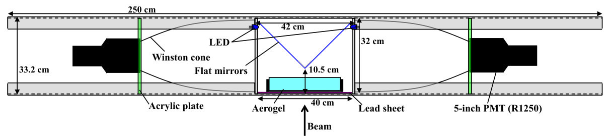
4.7.3.2 Expected counting rate and accidental loss in KOTO step-2
A single module is sensitive to 1-MeV photons. The incident rate of photons is 0.75 GHz for the energy larger than 1 MeV. If the detection efficiency is %, the hit rate is MHz.
We injected all the particles collected in the beam-line simulation to the beam-hole photon-veto counter with 25 modules. A full shower simulation and optical-photon tracking to the PMTs were performed, and the observed number of photoelectrons was recorded. For the module hit, “OR” of the PMTs on both sides is used for a certain photoelectron (p.e.) threshold. Consecutive three-module coincidence with a certain p.e. threshold (counter rate) was also calculated. Those module hit-rate and the consecutive three-module-coincidence rate (counter rate) are already shown in Fig. 163 for the 5.5-p.e. threshold as a base design. Those for the 0.5-p.e. threshold are shown in Fig. 184. Average module hit-rate in 2-sec spill is more than 30 MHz. The counter rate at the default threshold is . The resultant accidental loss is 19% with the 6-ns veto window, which correspond to of the timing resolution of 0.59 ns. It was achieved with the beam-hole photon-veto counter at KOTO step-1 by requiring the three-module coincidence with the 2.5-p.e. threshold [1309].

4.7.3.3 PMT operation and expected waveforms
We evaluated the average PMT-anode current in Fig. 185(a) based on the p.e. yields from the full simulation with the particles in the beam (Module ID 10 for example in Fig. 185(b)). A gain of the PMT is assumed. In more than half of PMTs, the anode currents exceed the maximum rating (0.2 mA) of the current PMT used in KOTO step-1. We may use a pre-amplifier to reduce the gain of the PMT and keep the single-p.e.sensitivity.


Expected waveforms after summing up the PMTs on both sides are shown in Fig. 186. In each panel, 10 waveforms are overlaid. The waveforms do overlap, but peaks can still be separated thus photons can be vetoed. Thus, we can still operate the beam-hole photon-veto counter in KOTO step-2 despite the harsh environment.


4.8 Conclusion
Measurement of the CP-violating rare decay mode plays an important role in the study of the flavor physics. It is one of the best probes for physics beyond the Standard Model. Following the ongoing search by the KOTO experiment, which will reach the sensitivity of better than in 3–4 years, KOTO step-2 is discussed and designed aiming to observe several tens of signals. To achieve more than 100 times better sensitivity than KOTO step-1, a new beam line with the production angle of 5 degrees is needed and could be accommodated in the Hadron Experimental Facility Extension project.
We evaluate the experimental sensitivity and the background level with a modeled beam line and detector. With a total of protons on target, which is equivalent to seconds of running with the 100 kW proton beam power, observation of 35 Standard Model (SM) events is expected. The corresponding single event sensitivity is . The estimated number of background events is 56, which corresponds to the signal-to-background ratio of 0.63. The significance of the observation for SM events is expected to be 4.7 .
Moving forward beyond the discussed base design for better sensitivity and signal acceptance, we continue to study and optimize many known effects and techniques including R&D of possible new detectors and analysis methods. This importance of the physics deserves a world class experiment (KOTO step-2) at the world class accelerator facility (J-PARC and Extended Hadron Experimental Facility).
References
- [985] S. Nagamiya In Nucl. Phys. A774, 2006, pp. 895 DOI: 10.1016/j.nuclphysa.2006.06.160
- [986] Shoji Nagamiya In Prog. Theor. Exp. Phys. 2012, 2012, pp. 02B001 DOI: 10.1093/ptep/pts025
- [987] B.. Abbott In Phys. Rev. Lett. 119, 2017, pp. 161101 DOI: 10.1103/PhysRevLett.119.161101
- [988] Andrzej. Buras, Dario Buttazzo, Jennifer Girrbach-Noe and Robert Knegjens In J. High Energy Phys., 2015, pp. 033 DOI: 10.1007/JHEP11(2015)033
- [989] Keizo Agari In Prog. Theor. Exp. Phys. 2012, 2012, pp. 02B008 DOI: 10.1093/ptep/pts034
- [990] Taku Yamanaka In Prog. Theor. Exp. Phys. 2012, 2012, pp. 02B006 DOI: 10.1093/ptep/pts057
- [991] Keizo Agari In Prog. Theor. Exp. Phys. 2012, 2012, pp. 02B009 DOI: 10.1093/ptep/pts038
- [992] Hiroyuki Fujioka, 2017 arXiv:1706.07916 [nucl-ex]
- [993] Hadron’, 2019 arXiv:1906.02357 [nucl-ex]
- [994] Tadashi Koseki In Prog. Theor. Exp. Phys. 2012, 2012, pp. 02B004 DOI: 10.1093/ptep/pts071
- [995] M. Moritsu In Phys. Rev. C90, 2014, pp. 035205 DOI: 10.1103/PhysRevC.90.035205
- [996] R. Honda In Phys. Rev. C96, 2017, pp. 014005 DOI: 10.1103/PhysRevC.96.014005
- [997] Toru Harada, Ryotaro Honda and Yoshiharu Hirabayashi In Phys. Rev. C 97, 2018, pp. 024601 DOI: 10.1103/PhysRevC.97.024601
- [998] Y. Ichikawa In Prog. Theor. Exp. Phys. 2015, 2015, pp. 021D01 DOI: 10.1093/ptep/ptv002
- [999] T.. Yamamoto In Phys. Rev. Lett. 115, 2015, pp. 222501 DOI: 10.1103/PhysRevLett.115.222501
- [1000] S.. Yang In Phys. Rev. Lett. 120, 2018, pp. 132505 DOI: 10.1103/PhysRevLett.120.132505
- [1001] T. Yamaga In Phys. Rev. C 102, 2020, pp. 044002 DOI: 10.1103/PhysRevC.102.044002
- [1002] T. Nagae In AIP Conf. Proc. 2130, 2019, pp. 020015 DOI: 10.1063/1.5118383
- [1003] S. Kawasaki In JPS Conf. Proc. 26, 2019, pp. 022009 DOI: 10.7566/JPSCP.26.022009
- [1004] H. Ekawa In Prog. Theor. Exp. Phys. 2019, 2019, pp. 021D02 DOI: 10.1093/ptep/pty149
- [1005] S.. Hayakawa In Phys. Rev. Lett. 126, 2021, pp. 062501 DOI: 10.1103/PhysRevLett.126.062501
- [1006] M. Yoshimoto In Prog. Theor. Exp. Phys. 2021, 2021, pp. 073D02 DOI: 10.1093/ptep/ptab073
- [1007] K. Miwa, 2021 arXiv:2104.13608 [nucl-ex]
- [1008] J.. Ahn In Phys. Rev. Lett. 126, 2021, pp. 121801 DOI: 10.1103/PhysRevLett.126.121801
- [1009] H. Ohnishi, F. Sakuma and T. Takahashi In Prog. Part. Nucl. Phys. 113, 2020, pp. 103773 DOI: 10.1016/j.ppnp.2020.103773
- [1010] Y. Ichikawa In Prog. Theor. Exp. Phys. 2020, 2020, pp. 123D01 DOI: 10.1093/ptep/ptaa139
- [1011] H. Sugimura In Phys. Lett. B729, 2014, pp. 39 DOI: 10.1016/j.physletb.2013.12.062
- [1012] K. Shirotori In Phys. Rev. Lett. 109, 2012, pp. 132002 DOI: 10.1103/PhysRevLett.109.132002
- [1013] Yudai Ichikawa In Prog. Theor. Exp. Phys. 2014, 2014, pp. 101D03 DOI: 10.1093/ptep/ptu128
- [1014] T. Hashimoto In Prog. Theor. Exp. Phys. 2015, 2015, pp. 061D01 DOI: 10.1093/ptep/ptv076
- [1015] Y. Sada In Prog. Theor. Exp. Phys. 2016, 2016, pp. 051D01 DOI: 10.1093/ptep/ptw040
- [1016] S. Ajimura In Phys. Lett. B789, 2019, pp. 620 DOI: 10.1016/j.physletb.2018.12.058
- [1017] H. Asano In AIP Conf. Proc. 2130, 2019, pp. 040018 DOI: 10.1063/1.5118415
- [1018] S. Okada In Prog. Theor. Exp. Phys. 2016, 2016, pp. 091D01 DOI: 10.1093/ptep/ptw130
- [1019] T. Hashimoto In JPS Conf. Proc. 26, 2019, pp. 023013 DOI: 10.7566/JPSCP.26.023013
- [1020] J.. Ahn In Prog. Theor. Exp. Phys. 2017, 2017, pp. 021C01 DOI: 10.1093/ptep/ptx001
- [1021] J.. Ahn In Phys. Rev. Lett. 122, 2019, pp. 021802 DOI: 10.1103/PhysRevLett.122.021802
- [1022] N. Shimizu In Phys. Rev. D102, 2020, pp. 051103(R) DOI: 10.1103/PhysRevD.102.051103
- [1023] H. Ito, 2021 arXiv:2107.03583 [hep-ex]
- [1024] H Takahashi In J. Radioanal. Nucl. Chem. 305, 2015, pp. 803 DOI: 10.1007/s10967-015-3940-9
- [1025] Hiroaki Watanabe In JPS Conf. Proc. 28, 2020, pp. 041004 DOI: 10.7566/JPSCP.28.041004
- [1026] Paul. Demorest et al. In Nature 467, 2010, pp. 1081 DOI: 10.1038/nature09466
- [1027] John Antoniadis In Science 340, 2013, pp. 1233232 DOI: 10.1126/science.1233232
- [1028] The CLAS Collaboration In Nature 560, 2018, pp. 617 DOI: 10.1038/s41586-018-0400-z
- [1029] Bao-An Li, Bao-Jun Cai, Lie-Wen Chen and Jun Xu In Prog. in Part. and Nucl. Phys. 99, 2018, pp. 29 DOI: 10.1016/j.ppnp.2018.01.001
- [1030] Megumi Naruki and Kotaro Shirotori In KEK/J-PARC-PAC 2014-4 2014-4, 2014
- [1031] S.. Kim et al. In Prog. Theor. Exp. Phys. 2014, 2014, pp. 103D01 DOI: 10.1093/ptep/ptu131
- [1032] Sang-In Shim, Atsushi Hosaka and Hyun-Chul Kim In Prog. Theor. Exp. Phys. 2020, 2020, pp. 053D01 DOI: 10.1093/ptep/ptaa049
- [1033] Georges Aad In Phys. Lett. B 716, 2012, pp. 1 DOI: 10.1016/j.physletb.2012.08.020
- [1034] Serguei Chatrchyan In Phys. Lett. B 716, 2012, pp. 30 DOI: 10.1016/j.physletb.2012.08.021
- [1035] B. Abi In Phys. Rev. Lett. 126, 2021, pp. 141801 DOI: 10.1103/PhysRevLett.126.141801
- [1036] Hideaki Hotchi In Prog. Theor. Exp. Phys. 2012, 2012, pp. 02B003 DOI: 10.1093/ptep/pts021
- [1037] L. Tang In Phys. Rev. C 90, 2014, pp. 034320 DOI: 10.1103/PhysRevC.90.034320
- [1038] A. Esser In Phys. Rev. Lett. 114, 2015, pp. 232501 DOI: 10.1103/PhysRevLett.114.232501
- [1039] L. Adamczyk In Phys. Rev. Lett. 114, 2015, pp. 022301 DOI: 10.1103/PhysRevLett.114.022301
- [1040] Shreyasi Acharya In Phys. Rev. C 99, 2019, pp. 024001 DOI: 10.1103/PhysRevC.99.024001
- [1041] Kenji Morita, Takenori Furumoto and Akira Ohnishi In Phys. Rev. C 91, 2015, pp. 024916 DOI: 10.1103/PhysRevC.91.024916
- [1042] Shreyasi Acharya In Phys. Lett. B 805, 2020, pp. 135419 DOI: 10.1016/j.physletb.2020.135419
- [1043] J. Rowley, 2021 arXiv:2108.03134 [hep-ex]
- [1044] Eduardo Cortina In J. High Energy Phys. 06, 2021, pp. 093 DOI: 10.1007/JHEP06(2021)093
- [1045] Matthew Moulson In J. Phys. Conf. Ser. 1526, 2020, pp. 012028 DOI: 10.1088/1742-6596/1526/1/012028
- [1046] M.. Miller In The Astrophysical Journal 887, 2019, pp. L24 DOI: 10.3847/2041-8213/ab50c5
- [1047] B.. Abbott In Phys. Rev. Lett. 121, 2018, pp. 161101 DOI: 10.1103/PhysRevLett.121.161101
- [1048] J.. Lattimer In Ann. Rev. Nucl. Part. Sci. 62, 2012, pp. 485 DOI: 10.1146/annurev-nucl-102711-095018
- [1049] T. Hasegawa In Phys. Rev. C 53, 1996, pp. 1210 DOI: 10.1103/PhysRevC.53.1210
- [1050] O Hashimoto and H Tamura In Prog. Part. Nucl. Phys. 57, 2006, pp. 564 DOI: 10.1016/j.ppnp.2005.07.001
- [1051] Gal. A., E.. Hungerford and D.. Millener In Rev. Mod. Phys. 88, 2016, pp. 035004 DOI: 10.1103/RevModPhys.88.035004
- [1052] I. Vidana et al. In Phys. Rev. C 61, 2000, pp. 025802 DOI: 10.1103/PhysRevC.61.025802
- [1053] H.-J. Schulze and T. Rijken In Phys. Rev. C 84, 2011, pp. 035801 DOI: 10.1103/PhysRevC.84.035801
- [1054] Haris Djapo, Bernd-Jochen Schaefer and Jochen Wambach In Phys. Rev. C 81, 2010, pp. 035803 DOI: 10.1103/PhysRevC.81.035803
- [1055] H.. Cromartie In Nature Astronomy 4, 2020, pp. 72 DOI: 10.1038/s41550-019-0880-2
- [1056] Robert. Wiringa, V… Stoks and R. Schiavilla In Phys. Rev. C 51, 1995, pp. 38 DOI: 10.1103/PhysRevC.51.38
- [1057] Robert. Wiringa and Steven. Pieper In Phys. Rev. Lett. 89, 2002, pp. 182501 DOI: 10.1103/PhysRevLett.89.182501
- [1058] J. Fujita and H. Miyazawa In Prog. Theor. Phys. 17, 1957, pp. 360 DOI: 10.1143/PTP.17.360
- [1059] K. Sekiguchi In Phys. Rev. C 65, 2002, pp. 034003 DOI: 10.1103/PhysRevC.65.034003
- [1060] A. Akmal, V.. Pandharipande and D.. Ravenhall In Phys. Rev. C 58, 1998, pp. 1804 DOI: 10.1103/PhysRevC.58.1804
- [1061] B.. Pudliner, V.. Pandharipande, J. Carlson and Robert. Wiringa In Phys. Rev. Lett. 74, 1995, pp. 4396 DOI: 10.1103/PhysRevLett.74.4396
- [1062] B.. Pudliner et al. In Phys. Rev. C 56, 1997, pp. 1720 DOI: 10.1103/PhysRevC.56.1720
- [1063] J. Carlson et al. In Rev. Mod. Phys. 87, 2015, pp. 1067 DOI: 10.1103/RevModPhys.87.1067
- [1064] M. Oertel, M. Hempel, T. Klähn and S. Typel In Rev. Mod. Phys. 89, 2017, pp. 015007 DOI: 10.1103/RevModPhys.89.015007
- [1065] Kota Masuda, Tetsuo Hatsuda and Tatsuyuki Takatsuka In The Astrophysical Journal 764, 2013, pp. 12 DOI: 10.1088/0004-637x/764/1/12
- [1066] Gordon Baym et al. In Rept. Prog. Phys. 81, 2018, pp. 056902 DOI: 10.1088/1361-6633/aaae14
- [1067] V… Stoks, R… Klomp, C… Terheggen and J.. de Swart In Phys. Rev. C 49, 1994, pp. 2950 DOI: 10.1103/PhysRevC.49.2950
- [1068] R. Machleidt In Phys. Rev. C 63, 2001, pp. 024001 DOI: 10.1103/PhysRevC.63.024001
- [1069] M.. Nagels, Th.. Rijken and Y. Yamamoto In Phys. Rev. C 99, 2019, pp. 044003 DOI: 10.1103/PhysRevC.99.044003
- [1070] Y. Yamamoto, T. Furumoto, N. Yasutake and Th.. Rijken In Phys. Rev. C 90, 2014, pp. 045805 DOI: 10.1103/PhysRevC.90.045805
- [1071] Y. Yamamoto, T. Furumoto, N. Yasutake and TH.. Rijken In Phys. Rev. C 88, 2013, pp. 022801 DOI: 10.1103/PhysRevC.88.022801
- [1072] T. Motoba, H. Bandō, R. Wünsch and J. Žofka In Phys. Rev. C 38, 1988, pp. 1322 DOI: 10.1103/PhysRevC.38.1322
- [1073] J. Haidenbauer et al. In Nucl. Phys. A 915, 2013, pp. 24 DOI: 10.1016/j.nuclphysa.2013.06.008
- [1074] Hoai Le, Johann Haidenbauer, Ulf-G. Meißner and Andreas Nogga In Phys. Lett. B 801, 2020, pp. 135189 DOI: 10.1016/j.physletb.2019.135189
- [1075] J. Haidenbauer, Ulf-G. Meißner and A. Nogga In Eur. Phys. J. A 56, 2020, pp. 91 DOI: 10.1140/epja/s10050-020-00100-4
- [1076] R. Wirth and R. Roth In Phys. Rev. Lett. 117, 2016, pp. 182501 DOI: 10.1103/PhysRevLett.117.182501
- [1077] Hoai Le, Johann Haidenbauer, Ulf-G. Meißner and Andreas Nogga In Eur. Phys. J. A 56, 2020, pp. 301 DOI: 10.1140/epja/s10050-020-00314-6
- [1078] Stefan Petschauer et al. In Phys. Rev. C 93, 2016, pp. 014001 DOI: 10.1103/PhysRevC.93.014001
- [1079] N. Ishii, S. Aoki and T. Hatsuda In Phys. Rev. Lett. 99, 2007, pp. 022001 DOI: 10.1103/PhysRevLett.99.022001
- [1080] Sinya Aoki et al. In Prog. Theor. Exp. Phys. 2012, 2012, pp. 01A105 DOI: 10.1093/ptep/pts010
- [1081] Takumi Iritani In Phys. Lett. B 792, 2019, pp. 284 DOI: 10.1016/j.physletb.2019.03.050
- [1082] Shinya Gongyo In Phys. Rev. Lett. 120, 2018, pp. 212001 DOI: 10.1103/PhysRevLett.120.212001
- [1083] E. Hiyama et al. In Phys. Rev. Lett. 124, 2020, pp. 092501 DOI: 10.1103/PhysRevLett.124.092501
- [1084] Takumi Doi et al. In Prog. Theor. Phys. 127, 2012, pp. 723 DOI: 10.1143/PTP.127.723
- [1085] Shreyasi Acharya In Phys. Lett. B 797, 2019, pp. 134822 DOI: 10.1016/j.physletb.2019.134822
- [1086] Shreyasi Acharya In Phys. Rev. Lett. 123, 2019, pp. 112002 DOI: 10.1103/PhysRevLett.123.112002
- [1087] M. Isaka, Y. Yamamoto and Th.. Rijken In Phys. Rev. C 94, 2016, pp. 044310 DOI: 10.1103/PhysRevC.94.044310
- [1088] M. Isaka, Y. Yamamoto and Th.. Rijken In presentation at JLab Hypernuclear workshop, 2016
- [1089] D. Lonardoni, F. Pederiva and S. Gandolfi In Phys. Rev. C 89, 2014, pp. 014314 DOI: 10.1103/PhysRevC.89.014314
- [1090] M. Oka and K. Yazaki In Phys. Lett. B 90, 1980, pp. 41 DOI: 10.1016/0370-2693(80)90046-5
- [1091] Makoto Oka, K. Shimizu and K. Yazaki In Prog. Theor. Phys. Suppl. 137, 2000, pp. 1 DOI: 10.1143/PTP.137.1
- [1092] K. Miwa In Proposal for J-PARC: Measurement of the differential cross section and spin observables of the scattering with a polarized beam, 2021
- [1093] R. Honda In Letter of Intent for J-PARC PAC: Measurement of cross section of the scattering, 2020
- [1094] T.. Yamamoto In Phys. Rev. Lett. 115, 2015, pp. 222501 DOI: 10.1103/PhysRevLett.115.222501
- [1095] J. Haidenbauer, Ulf-G. Meißner, N. Kaiser and W. Weise In Eur. Phys. J. A 53, 2017, pp. 121 DOI: 10.1140/epja/i2017-12316-4
- [1096] S.. Nakamura In Proposal for J-PARC: High precision spectroscopy of hypernuclei with the () reaction at the High Intensity High Resolution beamline, 2021
- [1097] B.. Sjögren In Nucl. Instrum. and Meth. 7, 1960, pp. 76 DOI: 10.1016/0029-554X(60)90073-2
- [1098] Y. Fujita In Nucl. Instrum. and Meth. B 126, 1997, pp. 274 DOI: 10.1016/S0168-583X(96)01008-7
- [1099] M. Fujiwara In Nucl. Instrum. and Meth. A 422, 1999, pp. 484 DOI: 10.1016/S0168-9002(98)01009-2
- [1100] L. Tang In JLab PAC35 Proposal PR12-10-001, 2010
- [1101] Avraham Gal and D.. Millener In Phys. Lett. B 725, 2013, pp. 445 DOI: 10.1016/j.physletb.2013.07.027
- [1102] P.. Pile In Phys. Rev. Lett. 66, 1991, pp. 2585 DOI: 10.1103/PhysRevLett.66.2585
- [1103] T. Hasegawa In Phys. Rev. Lett. 74, 1995, pp. 224 DOI: 10.1103/PhysRevLett.74.224
- [1104] S. Ajimura In Nucl. Phys. A 639, 1998, pp. 93 DOI: 10.1016/S0375-9474(98)00255-3
- [1105] H. Hotchi In Phys. Rev. C 64, 2001, pp. 044302 DOI: 10.1103/PhysRevC.64.044302
- [1106] T. Gogami In Nucl. Instrum. Meth. A 900, 2018, pp. 69 DOI: 10.1016/j.nima.2018.05.042
- [1107] H. Thiessem In BNL-AGS Proposal E758, 1980
- [1108] C. Milner In Phys. Rev. Lett. 54, 1985, pp. 1237 DOI: 10.1103/PhysRevLett.54.1237
- [1109] Toshio Motoba, Kazunori Itonaga and Yasuo Yamamoto In Prog. Theor. Phys. Suppl. 185, 2010, pp. 197 DOI: 10.1143/PTPS.185.197
- [1110] Peter.. Pang et al., 2021 arXiv:2105.08688 [astro-ph.HE]
- [1111] G. Raaijmakers, 2021 arXiv:2105.06981 [astro-ph.HE]
- [1112] Ignazio Bombaci In JPS Conf. Proc. 17, 2017, pp. 101002 DOI: 10.7566/JPSCP.17.101002
- [1113] V.. Ambartsumyan and G.. Saakyan In Sov. Astron. AJ 4, 1960, pp. 187
- [1114] S.. Thorsett and Deepto Chakrabarty In Astrophys. J. 512, 1999, pp. 288 DOI: 10.1086/306742
- [1115] John Antoniadis In Science 340, 2013, pp. 6131 DOI: 10.1126/science.1233232
- [1116] Isaac Vidana et al. In EPL 94, 2011, pp. 11002 DOI: 10.1209/0295-5075/94/11002
- [1117] E. Massot, J. Margueron and G. Chanfray In Europhys. Lett. 97, 2012, pp. 39002 DOI: 10.1209/0295-5075/97/39002
- [1118] I. Bednarek In Astron. Astrophys. A157, 2012, pp. 543 DOI: 10.1051/0004-6361/201118560
- [1119] Simon Weissenborn, Debarati Chatterjee and Juergen Schaffner-Bielich In Phys. Rev. C 85, 2012, pp. 065802 DOI: 10.1103/PhysRevC.85.065802
- [1120] Tsuyoshi Miyatsu, Myung-Ki Cheoun and Koichi Saito In Phys. Rev. C 88, 2013, pp. 015802 DOI: 10.1103/PhysRevC.88.015802
- [1121] Luiz. Lopes and Debora. Menezes In Phys. Rev. C 89, 2014, pp. 025805 DOI: 10.1103/PhysRevC.89.025805
- [1122] R. Machleidt, F. Sammarruca and Y. Song In Phys. Rev. C 53, 1996, pp. R1483 DOI: 10.1103/PhysRevC.53.R1483
- [1123] E. Epelbaum, W. Glöckle and Ulf-G Meißner In Nucl. Phys. A 747, 2005, pp. 362 DOI: 10.1016/j.nuclphysa.2004.09.107
- [1124] A. Ekström In Phys. Rev. Lett. 110, 2013, pp. 192502 DOI: 10.1103/PhysRevLett.110.192502
- [1125] J. Hoppe et al. In Phys. Rev. C 96, 2017, pp. 054002 DOI: 10.1103/PhysRevC.96.054002
- [1126] K. Miwa In J-PARC E40 experiment.
- [1127] S. Gandolfi, J. Carlson and Sanjay Reddy In Phys. Rev. C 85, 2012, pp. 032801 DOI: 10.1103/PhysRevC.85.032801
- [1128] S. Gandolfi, J. Carlson and S. Reddy In Eur. Phys. J. A 50, 2014, pp. 10 DOI: 10.1140/epja/i2014-14010-5
- [1129] M.. Nagels, Th.. Rijken and Y. Yamamoto In Phys. Rev. C 99, 2019, pp. 044002 DOI: 10.1103/PhysRevC.99.044002
- [1130] T. Furumoto, Y. Sakuragi and Y. Yamamoto In Phys. Rev. C 79, 2009, pp. 011601 DOI: 10.1103/PhysRevC.79.011601
- [1131] Diego Lonardoni, Alessandro Lovato, Stefano Gandolfi and Francesco Pederiva In Phys. Rev. Lett. 114, 2015, pp. 092301 DOI: 10.1103/PhysRevLett.114.092301
- [1132] Thomas. Rijken, M.. Nagels and Yasuo Yamamoto In Prog. Theor. Phys. Suppl. 185, 2010, pp. 14 DOI: 10.1143/PTPS.185.14
- [1133] A. Reuber, K. Holinde and J. Speth In Nucl. Phys. A 570, 1994, pp. 543 DOI: 10.1016/0375-9474(94)90073-6
- [1134] J. Haidenbauer and Ulf-G. Meißner In Phys. Rev. C 72, 2005, pp. 044005 DOI: 10.1103/PhysRevC.72.044005
- [1135] S. Aoki In Prog. Theor. Phys. 123, 2010, pp. 89 DOI: 10.1143/PTP.123.89
- [1136] S. Aoki In Proc. Jpn. Acad. B87, 2011, pp. 509 DOI: 10.2183/pjab.87.509
- [1137] N. Ishii In Phys. Lett. B 712, 2012, pp. 437 DOI: 10.1016/j.physletb.2012.04.076
- [1138] Roland Wirth, Daniel Gazda, Petr Navrátil and Robert Roth In Phys. Rev. C 97, 2018, pp. 064315 DOI: 10.1103/PhysRevC.97.064315
- [1139] E. Hiyama and T. Yamada In Prog. Part. Nucl. Phys. 63, 2009, pp. 339 DOI: 10.1016/j.ppnp.2009.05.001
- [1140] T.. Rijken, V… Stoks and Y. Yamamoto In Phys. Rev. C 59, 1999, pp. 21 DOI: 10.1103/PhysRevC.59.21
- [1141] T. Gogami In Phys. Rev. C 93, 2016, pp. 034314 DOI: 10.1103/PhysRevC.93.034314
- [1142] E. Botta, T. Bressani and A. Feliciello In Nucl. Phys. A 960, 2017, pp. 165 DOI: 10.1016/j.nuclphysa.2017.02.005
- [1143] M. Isaka, Y. Yamamoto and Th.. Rijken In Phys. Rev. C 95, 2017, pp. 044308 DOI: 10.1103/PhysRevC.95.044308
- [1144] Francesco Pederiva et al., 2015 arXiv:1506.04042 [nucl-th]
- [1145] A.. Bodmer, Q.. Usmani and J. Carlson In Phys. Rev. C 29, 1984, pp. 684 DOI: 10.1103/PhysRevC.29.684
- [1146] A.. Usmani, S.. Pieper and Q.. Usmani In Phys. Rev. C 51, 1995, pp. 2347 DOI: 10.1103/PhysRevC.51.2347
- [1147] A.. Usmani In Phys. Rev. C 52, 1995, pp. 1773 DOI: 10.1103/PhysRevC.52.1773
- [1148] Q.. Usmani and A.. Bodmer In Phys. Rev. C 60, 1999, pp. 055215 DOI: 10.1103/PhysRevC.60.055215
- [1149] F. Ferrari et al. In Few Body Syst. 58, 2017, pp. 113 DOI: 10.1007/s00601-017-1273-7
- [1150] M. Imran et al. In J. Phys. G 41, 2014, pp. 065101 DOI: 10.1088/0954-3899/41/6/065101
- [1151] Henk Polinder, Johann Haidenbauer and Ulf-G. Meißner In Nucl. Phys. A 779, 2006, pp. 244 DOI: 10.1016/j.nuclphysa.2006.09.006
- [1152] M. Kohno In Phys. Rev. C 97, 2018, pp. 035206 DOI: 10.1103/PhysRevC.97.035206
- [1153] Dominik Gerstung, Norbert Kaiser and Wolfram Weise In Eur. Phys. J. A 56, 2020, pp. 175 DOI: 10.1140/epja/s10050-020-00180-2
- [1154] P. Navratil, J.. Vary and B.. Barrett In Phys. Rev. C 62, 2000, pp. 054311 DOI: 10.1103/PhysRevC.62.054311
- [1155] E. Hiyama et al. In Phys. Rev. C 65, 2002, pp. 011301 DOI: 10.1103/PhysRevC.65.011301
- [1156] Daniel Gazda and Avraham Gal In Nucl. Phys. A 954, 2016, pp. 161 DOI: 10.1016/j.nuclphysa.2016.05.015
- [1157] Andreas Nogga In AIP Conf. Proc. 2130, 2019, pp. 030004 DOI: 10.1063/1.5118394
- [1158] S.. Nakamura In Phys. Rev. Lett. 110, 2013, pp. 012502 DOI: 10.1103/PhysRevLett.110.012502
- [1159] T. Gogami In Phys. Rev. C 94, 2016, pp. 021302 DOI: 10.1103/PhysRevC.94.021302
- [1160] T. Gogami In Phys. Rev. C 103, 2021, pp. L041301 DOI: 10.1103/PhysRevC.103.L041301
- [1161] T. Motoba In Special talk at the JPS Meeting, 2021
- [1162] Masahiro Isaka, Masaaki Kimura, Akinobu Doté and Akira Ohnishi In Phys. Rev. C 87, 2013, pp. 021304 DOI: 10.1103/PhysRevC.87.021304
- [1163] T. Yamazaki In KEK Report 84-20, 1984, pp. 3
- [1164] Kazuo Tsushima, K. Saito, Johann Haidenbauer and Anthony Thomas In Nucl. Phys. A 630, 1998, pp. 691 DOI: 10.1016/S0375-9474(98)00806-9
- [1165] C.. Keil, F. Hofmann and H. Lenske In Phys. Rev. C 61, 2000, pp. 064309 DOI: 10.1103/PhysRevC.61.064309
- [1166] C.. Dover In Proceedings of International Symposium on Medium Energy Physics, 1987, pp. BNL–40074
- [1167] Bernard Frois and Costas. Papanicolas In Ann. Rev. Nucl. Part. Sci. 37, 1987, pp. 133 DOI: 10.1146/annurev.nucl.37.1.133
- [1168] T. Takahashi In Prog. Theor. Exp. Phys. 2012, 2012, pp. 02B010 DOI: 10.1093/ptep/pts023
- [1169] J.R. Sanford and C.L. Wang In BNL internal reports Nos. 11299 and 11479, 1962
- [1170] C.. Wang In Phys. Rev. Lett. 25, 1970, pp. 1068 DOI: 10.1103/PhysRevLett.25.1068
- [1171] H. Fujioka In HIHR/K1.1 workshop, 2021
- [1172] S. Nagao In presentation at International workshop on the project for the extended hadron experimental facility of J-PARC, March 27, 2018, 2018
- [1173] T. Hasegawa In INS-IM-15, 1994
- [1174] Y. Akaishi, Khin Myint, T. Harada and S. Shinmura In Phys. Rev. Lett. 84, 2000, pp. 3539 DOI: 10.1103/PhysRevLett.84.3539
- [1175] I. Tanihata et al. In Phys. Rev. Lett. 55, 1985, pp. 2676 DOI: 10.1103/PhysRevLett.55.2676
- [1176] T. Kobayashi et al. In Phys. Rev. Lett. 60, 1988, pp. 2599 DOI: 10.1103/PhysRevLett.60.2599
- [1177] E. Hiyama In Few Body Syst. 34, 2004, pp. 79 DOI: 10.1007/s00601-004-0024-8
- [1178] P.. Saha In Phys. Rev. Lett. 94, 2005, pp. 052502 DOI: 10.1103/PhysRevLett.94.052502
- [1179] M. Agnello In Phys. Lett. B 640, 2006, pp. 145 DOI: 10.1016/j.physletb.2006.07.051
- [1180] M. Agnello In Phys. Rev. Lett. 108, 2012, pp. 042501 DOI: 10.1103/PhysRevLett.108.042501
- [1181] H. Machner In Nucl. Phys. A 901, 2013, pp. 65 DOI: 10.1016/j.nuclphysa.2013.01.031
- [1182] R.. Dalitz In Nucl. Phys. A 354, 1981, pp. 101 DOI: 10.1016/0375-9474(81)90595-9
- [1183] R.. Dalitz and A. Deloff In Czech. J. Phys. B, 1982, pp. 32 DOI: 10.1007/BF01597174
- [1184] A. Budzanowski In Phys. Lett. B692, 2010, pp. 10 DOI: 10.1016/j.physletb.2010.07.015
- [1185] T. Motoba, K. Itonaga and H. BandŌ In Nucle. Phys. A 489, 1988, pp. 683 DOI: 10.1016/0375-9474(88)90116-9
- [1186] Y. Yamamoto et al. In Prog. Theor. Phys. Suppl. 117, 1994, pp. 361 DOI: 10.1143/ptp.117.361
- [1187] M. Agnello In Phys. Lett. B 681, 2009, pp. 139 DOI: 10.1016/j.physletb.2009.09.061
- [1188] H. Homma, M. Isaka and M. Kimura In Phys. Rev. C 91, 2015, pp. 014314 DOI: 10.1103/PhysRevC.91.014314
- [1189] R.. Chrien In Phys. Rev. Lett. 60, 1988, pp. 2595 DOI: 10.1103/PhysRevLett.60.2595
- [1190] Y.. Tanaka In Phys. Rev. Lett. 117, 2016, pp. 202501 DOI: 10.1103/PhysRevLett.117.202501
- [1191] Y.. Tanaka In Phys. Rev. C 97, 2018, pp. 015202 DOI: 10.1103/PhysRevC.97.015202
- [1192] N. Tomida In Phys. Rev. Lett. 124, 2020, pp. 202501 DOI: 10.1103/PhysRevLett.124.202501
- [1193] K. Kisamori In Phys. Rev. Lett. 116, 2016, pp. 052501 DOI: 10.1103/PhysRevLett.116.052501
- [1194] H. Fujioka In Letter of Intent for J-PARC: Search for tetraneutron by pion double charge exchange reaction on 4He, 2016
- [1195] M. Oka, K. Shimizu and K. Yazaki In Nucl. Phys. A 464, 1987, pp. 700 DOI: 10.1016/0375-9474(87)90371-X
- [1196] Y. Fujiwara, Y. Suzuki and C. Nakamoto In Prog. Part. Nucl. Phys. 58, 2007, pp. 439 DOI: 10.1016/j.ppnp.2006.08.001
- [1197] T. Inoue In Nucl. Phys. A 881, 2012, pp. 28 DOI: 10.1016/j.nuclphysa.2012.02.008
- [1198] H. Nemura In EPJ Web of Conf. 175, 2018, pp. 05030 DOI: 10.1051/epjconf/201817505030
- [1199] B. Sechi-Zorn, B. Kehoe, J. Twitty and R.. Burnstein In Phys. Rev. 175, 1968, pp. 1735 DOI: 10.1103/PhysRev.175.1735
- [1200] G. Alexander In Phys. Rev. 173, 1968, pp. 1452 DOI: 10.1103/PhysRev.173.1452
- [1201] J.. Kadyk et al. In Nucl. Phys. B 27, 1971, pp. 13 DOI: 10.1016/0550-3213(71)90076-9
- [1202] J.. Hauptman, J.. Kadyk and G.. Trilling In Nucl. Phys. B 125, 1977, pp. 29 DOI: 10.1016/0550-3213(77)90222-X
- [1203] R. Engelmann, H. Filthuth, V. Hepp and E. Kluge In Phys. Lett. 21, 1966, pp. 587 DOI: 10.1016/0031-9163(66)91310-2
- [1204] F. Eisele et al. In Phys. Lett. B 37, 1971, pp. 204 DOI: 10.1016/0370-2693(71)90053-0
- [1205] D. Stephen In Ph.D. thesis, 1970
- [1206] Y. Kondo In Nucl. Phys. A 676, 2000, pp. 371 DOI: 10.1016/S0375-9474(00)00191-3
- [1207] J.. Ahn In Nucl. Phys. A 761, 2005, pp. 41 DOI: 10.1016/j.nuclphysa.2005.07.004
- [1208] Y. Yamamoto, T. Motoba and Th.. Rijken In Prog. Theor. Phys. Suppl. 185, 2010, pp. 72 DOI: 10.1143/PTPS.185.72
- [1209] K. Miwa In J. Phys. : Conf. Ser. 1643, 2020, pp. 012174 DOI: 10.1088/1742-6596/1643/1/012174
- [1210] S Ishikawa In Phys. Rev. C 69, 2004, pp. 034001 DOI: 10.1103/PhysRevC.69.034001
- [1211] J. Haidenbauer, K. Holinde, V. Mull and J. Speth In Phys. Lett. B 291, 1992, pp. 223 DOI: 10.1016/0370-2693(92)91035-8
- [1212] M. Kurosawa In Jps. J. Appl. Phys. 45, 2006, pp. 4204 DOI: 10.1143/jjap.45.4204
- [1213] J. Haidenbauer In private communication
- [1214] J. Haidenbauer and Ulf-G. Meißner, 2021 arXiv:2105.00836 [nucl-th]
- [1215] Th.. Rijken In private communication
- [1216] S. Petschauer et al. In Nucl. Phys. A 957, 2017, pp. 347 DOI: 10.1016/j.nuclphysa.2016.09.010
- [1217] J. Haidenbauer and I. Vidaña In Eur. Phys. J. A 56, 2020, pp. 55 DOI: 10.1140/epja/s10050-020-00055-6
- [1218] J.. Jones In Phys. Rev. Lett. 26, 1971, pp. 860 DOI: 10.1103/PhysRevLett.26.860
- [1219] T.. Knasel In Phys. Rev. D 11, 1975, pp. 1 DOI: 10.1103/PhysRevD.11.1
- [1220] T.. Binford In Phys. Rev. 183, 1969, pp. 1134 DOI: 10.1103/PhysRev.183.1134
- [1221] R.. Baker In Nucl. Phys. B 141, 1978, pp. 29 DOI: 10.1016/0550-3213(78)90332-2
- [1222] John. Price In AIP Conf. Proc. 2130, 2019, pp. 020004 DOI: 10.1063/1.5118372
- [1223] H. Tamura In Phys. Rev. Lett. 84, 2000, pp. 5963 DOI: 10.1103/PhysRevLett.84.5963
- [1224] D.J. Millener “Hypernuclear Gamma-Ray Spectroscopy and the Structure of p-shell Nuclei and Hypernuclei” In Topics in Strangeness Nuclear Physics Springer Berlin Heidelberg, 2007, pp. 31–79 DOI: 10.1007/978-3-540-72039-3˙2
- [1225] K. Tanida and otehrs In Phys. Rev. Lett. 86, 2001, pp. 1982 DOI: 10.1103/PhysRevLett.86.1982
- [1226] C. Rappold In Phys. Rev. C 88, 2013, pp. 041001 DOI: 10.1103/PhysRevC.88.041001
- [1227] H. Tamura, M. Ukai, T.. Yamamoto and T. Koike In Nucl. Phys. A 881, 2012, pp. 310 DOI: 10.1016/j.nuclphysa.2012.02.013
- [1228] K. Kamada, M. Fujita and H. Tamura In Letter of Intent for J-PARC: Modification of baryon structure in nuclear matter studied from beta-decay rate of a hypernucleus, 2021
- [1229] Alessandro Feliciello In AIP Conf. Proc. 2130, 2019, pp. 020020 DOI: 10.1063/1.5118388
- [1230] ALICE In Nucl. Phys. A 1005, 2021, pp. 121791 DOI: 10.1016/j.nuclphysa.2020.121791
- [1231] A. Feliciello and T. Nagae In Rept. Prog. Phys. 78, 2015, pp. 096301 DOI: 10.1088/0034-4885/78/9/096301
- [1232] H. Tamura In Nucl. Phys. A 691, 2001, pp. 86 DOI: 10.1016/S0375-9474(01)01012-0
- [1233] P.. Zyla In Prog. Theor. Exp. Phys. 2020, 2020, pp. 083C01 DOI: 10.1093/ptep/ptaa104
- [1234] M. Takayama, H. Toki and A. Hosaka In Prog. Theor. Phys. 101, 1999, pp. 1271 DOI: 10.1143/PTP.101.1271
- [1235] Dmitri Diakonov In Prog. Part. Nucl. Phys. 51, 2003, pp. 173 DOI: 10.1016/S0146-6410(03)90014-7
- [1236] Tom Banks and A. Casher In Nucl. Phys. B 169, 1980, pp. 103 DOI: 10.1016/0550-3213(80)90255-2
- [1237] Gerard ’t In Phys. Rev. Lett. 37, 1976, pp. 8 DOI: 10.1103/PhysRevLett.37.8
- [1238] Gerard ’t In Phys. Rev. D 14, 1976, pp. 3432 DOI: 10.1103/PhysRevD.14.3432
- [1239] M. Kobayashi and T. Maskawa In Prog. Theor. Phys. 44, 1970, pp. 1422 DOI: 10.1143/PTP.44.1422
- [1240] Kenji Fukushima and Tetsuo Hatsuda In Rept. Prog. Phys. 74, 2011, pp. 014001 DOI: 10.1088/0034-4885/74/1/014001
- [1241] Anthony. Thomas In Prog. Theor. Phys. 168, 2007, pp. 614 DOI: 10.1143/PTPS.168.614
- [1242] Yonghee Kim, Emiko Hiyama, Makoto Oka and Kei Suzuki In Phys. Rev. D 102, 2020, pp. 014004 DOI: 10.1103/PhysRevD.102.014004
- [1243] Hideko Nagahiro et al. In Phys. Rev. D 95, 2017, pp. 014023 DOI: 10.1103/PhysRevD.95.014023
- [1244] K.. Can, G. Erkol, M. Oka and T.. Takahashi In Phys. Rev. D 92, 2015, pp. 114515 DOI: 10.1103/PhysRevD.92.114515
- [1245] T. Yoshida et al. In Phys. Rev. D 92, 2015, pp. 114029 DOI: 10.1103/PhysRevD.92.114029
- [1246] Hiroyuki Noumi In KEK/J-PARC-PAC 2012-19, 2012
- [1247] D.. Crennell, H.. Gordon, Kwan-Wu Lai and J.. Scarr In Phys. Rev. D 6, 1972, pp. 1220 DOI: 10.1103/PhysRevD.6.1220
- [1248] Yohei Kawakami, Masayasu Harada, Makoto Oka and Kei Suzuki In Phys. Rev. D 102, 2020, pp. 114004 DOI: 10.1103/PhysRevD.102.114004
- [1249] Georg. Engel, C.. Lang, Daniel Mohler and Andreas Schäfer In Phys. Rev. D 87, 2013, pp. 074504 DOI: 10.1103/PhysRevD.87.074504
- [1250] Kuang-Ta Chao, Nathan Isgur and Gabriel Karl In Phys. Rev. D 23, 1981, pp. 155 DOI: 10.1103/PhysRevD.23.155
- [1251] Ahmad Arifi In private communication, 2021
- [1252] J.. Kinson In Proceedings of 4th International Conference on Baryon Resonances, 1980, pp. 263
- [1253] Murray Gell-Mann In Phys. Lett. 8, 1964, pp. 214 DOI: 10.1016/S0031-9163(64)92001-3
- [1254] V.. Barnes In Phys. Rev. Lett. 12, 1964, pp. 204 DOI: 10.1103/PhysRevLett.12.204
- [1255] J. Yelton In Phys. Rev. Lett. 121, 2018, pp. 052003 DOI: 10.1103/PhysRevLett.121.052003
- [1256] Ming-Sheng Liu, Kai-Lei Wang, Qi-Fang Lü and Xian-Hui Zhong In Phys. Rev. D 101, 2020, pp. 016002 DOI: 10.1103/PhysRevD.101.016002
- [1257] Sachiko Takeuchi In Nucl. Phys. A 642, 1998, pp. 543 DOI: 10.1016/S0375-9474(98)00539-9
- [1258] M. Valderrama In Phys. Rev. D 98, 2018, pp. 054009 DOI: 10.1103/PhysRevD.98.054009
- [1259] Natsumi Ikeno, Genaro Toledo and Eulogio Oset In Phys. Rev. D 101, 2020, pp. 094016 DOI: 10.1103/PhysRevD.101.094016
- [1260] T.. Moon In Phys. Rev. D 103, 2021, pp. L111101 DOI: 10.1103/PhysRevD.103.L111101
- [1261] A.M. Sirunyan In Phys. Lett. B 803, 2020, pp. 135345 DOI: 10.1016/j.physletb.2020.135345
- [1262] Roel Aaij In J. High Energy Phys. 06, 2020, pp. 136 DOI: 10.1007/JHEP06(2020)136
- [1263] N.˜Suzuki, B.˜Juliá-Díaz, H.˜Kamano, T.˜S.˜H.˜Lee, A.˜Matsuyama and T.˜Sato In Phys. Rev. Lett. 104, 2010, pp. 042302 DOI: 10.1103/PhysRevLett.104.042302
- [1264] Volker. Burkert and Craig. Roberts In Rev. Mod. Phys. 91, 2019, pp. 011003 DOI: 10.1103/RevModPhys.91.011003
- [1265] Steven Weinberg In Phys. Rev. Lett. 65, 1990, pp. 1181 DOI: 10.1103/PhysRevLett.65.1181
- [1266] T. Kubota and K. Ohta In Phys. Lett. B 65, 1976, pp. 374 DOI: 10.1016/0370-2693(76)90246-X
- [1267] Ahmad Arifi, Daiki Suenaga and Atsushi Hosaka In Phys. Rev. D 103, 2021, pp. 094003 DOI: 10.1103/PhysRevD.103.094003
- [1268] B. Juliá-Díaz, D.. Riska and F. Coester In Phys. Rev. C 70, 2004, pp. 045204 DOI: 10.1103/PhysRevC.70.045204
- [1269] In http://aea.web.psi.ch/Urs_Rohrer/MyWeb/trans.htm
- [1270] K.. Tanaka et al. “Optical design of beam lines at the KEK PS new experimental hall” In Nucl. Instrum. Meth. A 363, 1995, pp. 114–119 DOI: 10.1016/0168-9002(95)00360-6
- [1271] In http://aea.web.psi.ch/Urs_Rohrer/MyWeb/turtle.htm
- [1272] T Aramaki In ELPH annual report, Tohoku University 2018, 2019, pp. 44
- [1273] T Akaishi In ELPH annual report, Tohoku University 2018, 2019, pp. 58
- [1274] M Naruki In RCNP annual report, Osaka University 2020, 2020
- [1275] Kotaro Shirotori In PoS (Hadron2013), 2013, pp. 130 DOI: 10.22323/1.205.0130
- [1276] Y Ma “Performance evaluation of the next generation DAQ system with high-rate detectors for the J-PARC E50 experiment” In Proposal for the ELPH experiment ELPH-2900, 2018
- [1277] R Honda “Continuous timing measurement using data streaming DAQ system” In Prog. Theor. Exp. Phys., 2021, pp. in press
- [1278] T. Ishikawa In Nucl. Instrum. Meth. A 622, 2010, pp. 1 DOI: 10.1016/j.nima.2010.07.051
- [1279] Y. Nara et al. In Phys. Rev. C 61, 2000, pp. 024901 DOI: 10.1103/PhysRevC.61.024901
- [1280] C.. Jenkins In Phys. Rev. Lett. 51, 1983, pp. 95 DOI: 10.1103/PhysRevLett.51.951
- [1281] Kenji Morita et al. In Phys. Rev. C 101, 2019, pp. 015201 DOI: 10.1103/PhysRevC.101.015201
- [1282] S. Acharya In Nature 588, 2020, pp. 232 DOI: 10.1038/s41586-020-3001-6
- [1283] Takayasu Sekihara, Yuki Kamiya and Tetsuo Hyodo In Phys. Rev. C 98, 2018, pp. 015205 DOI: 10.1103/PhysRevC.98.015205
- [1284] M. Jacob and G.. Wick In Ann. Phys. 7, 1959, pp. 404 DOI: 10.1016/0003-4916(59)90051-X
- [1285] L.. Copley, G. Karl and E. Obryk In Nucl. Phys. B 13, 1969, pp. 303 DOI: 10.1016/0550-3213(69)90237-5
- [1286] Torbjorn Sjostrand, Stephen Mrenna and Peter. Skands In Comput. Phys. Commun. 178, 2008, pp. 852 DOI: 10.1016/j.cpc.2008.01.036
- [1287] S.. Ganguli In Nucl. Phys. B 128, 1977, pp. 408 DOI: 10.1016/0550-3213(77)90053-0
- [1288] R.. Hemingway In Nucl. Phys. B 142, 1978, pp. 205 DOI: 10.1016/0550-3213(78)90197-9
- [1289] J.. Hassall et al. In Nucl. Phys. B 189, 1981, pp. 397 DOI: 10.1016/0550-3213(81)90572-1
- [1290] M. Baubillier In Nucl. Phys. B 192, 1981, pp. 1 DOI: 10.1016/0550-3213(81)90189-9
- [1291] P. Sixel In Nucl. Phys. B 159, 1979, pp. 125 DOI: 10.1016/0550-3213(79)90330-4
- [1292] D. Aston In Phys. Rev. D 32, 1985, pp. 2270 DOI: 10.1103/PhysRevD.32.2270
- [1293] Bo Andersson, G. Gustafson, G. Ingelman and T. Sjostrand In Phys. Rept. 97, 1983, pp. 31 DOI: 10.1016/0370-1573(83)90080-7
- [1294] L.. Biedenharn and M.. Rose In Rev. Mod. Phys. 25, 1953, pp. 729 DOI: 10.1103/RevModPhys.25.729
- [1295] K. Moriya In Phys. Rev. Lett. 112, 2014, pp. 082004 DOI: 10.1103/PhysRevLett.112.082004
- [1296] Andrzej. Buras, Dario Buttazzo, Jennifer Girrbach-Noe and Robert Knegjens In JHEP 11, 2014, pp. 121 DOI: 10.1007/JHEP11(2014)121
- [1297] Andrzej. Buras, Dario Buttazzo, Jennifer Girrbach-Noe and Robert Knegjens In JHEP 11, 2015, pp. 033 DOI: 10.1007/JHEP11(2015)033
- [1298] Joachim Brod, Martin Gorbahn and Emmanuel Stamou In Phys. Rev. D 83, 2011, pp. 034030 DOI: 10.1103/PhysRevD.83.034030
- [1299] Yuval Grossman and Yosef Nir In Phys. Lett. B 398, 1997, pp. 163 DOI: 10.1016/S0370-2693(97)00210-4
- [1300] Andrzej. Buras, Dario Buttazzo and Robert Knegjens In JHEP 11, 2015, pp. 166 DOI: 10.1007/JHEP11(2015)166
- [1301] David Marzocca, Sokratis Trifinopoulos and Elena Venturini, 2021 arXiv:2106.15630 [hep-ph]
- [1302] J. Comfort “Proposal for Experiment at J-PARC”, 2006
- [1303] Tadashi Nomura In J. Phys. Conf. Ser. 1526, 2020, pp. 012027 DOI: 10.1088/1742-6596/1526/1/012027
- [1304] Tetsushi Shimogawa In Nucl. Instrum. Meth. A 623, 2010, pp. 585 DOI: 10.1016/j.nima.2010.03.078
- [1305] R. Murayama In Nucl. Instrum. Meth. A 953, 2020, pp. 163255 DOI: 10.1016/j.nima.2019.163255
- [1306] K. Sato In Nucl. Instrum. Meth. A 982, 2020, pp. 164527 DOI: 10.1016/j.nima.2020.164527
- [1307] D. Naito In PTEP 2016, 2016, pp. 023C01 DOI: 10.1093/ptep/ptv191
- [1308] I. Kamiji and K. Nakagiri In J. Phys. Conf. Ser. 800, 2017, pp. 012041 DOI: 10.1088/1742-6596/800/1/012041
- [1309] Y. Maeda In PTEP 2015, 2015, pp. 063H01 DOI: 10.1093/ptep/ptv074
- [1310] “KOPIO Conceptual Design Report”, 2005
- [1311] R.M. and D.J.A In Nucl. Instr. Meth. Phys. Res. A 666, 2012, pp. 47 DOI: 10.1016/j.nima.2011.03.017
- [1312] E. Iwai In Nucl. Instr. Meth. A 786, 2015, pp. 135 DOI: 10.1016/j.nima.2015.02.046