Fair Regression under Sample Selection Bias

We first define the notations used in this paper. Let $(\bm{X},A,Y)$ denote the training data $\mathcal{D}$, where $\bm{X}$ is the feature space, $A$ is the protected attribute, and $Y$ is the continuous target attribute. $\mathcal{D}$ contains $n$ data samples, among which $m$ samples $(\bm{x}_{i},a_{i},y_{i})$ are fully observed and the remaining $n-m$ data points have $y_{i}$ missing. We denote the fully observed part as $\mathcal{D}_{s}$ and the other part as $\mathcal{D}_{u}$. The whole training data $\mathcal{D}$ is selected uniformly from the population to be modeled. However, $\mathcal{D}_{s}$ is non-uniformly selected and the bias of $\mathcal{D}_{s}$ could depend on both feature vector $\bm{x},a$ and target variable $y$. A regression function $f(\cdot):X\rightarrow Y$ tries to learn optimal parameter $\bm{w}$. We denote $\hat{y}=f(\bm{x};\bm{w})$.

We emphasize the sample selection bias considered in our paper is different from the traditional covariate shift scenario. Although the covariate shift tackles the shift between the training distribution $P_{tr}(X)$ and test distribution $P_{te}(X)$, it usually assumes both a labeled training dataset and an unlabeled testing dataset are available in the training phase. In our work, we do not require the unlabeled testing data in the training phase. Instead, we assume the available training dataset contains a mixture of labeled and unlabeled data points but the labeling process is biased. In our setting, we are able to use the Heckman model to correct the bias with theoretical guarantee as we can compute the conditional unbiased expectation analytically. However, the previous commonly used approaches for covariate shift can only achieve robust estimation within a range but cannot provide theoretical guarantee.

Heckman model [15] addresses the issue of sample selection bias when the dependent variable in the regression has values that are missing not at random. In the two-step estimation procedure of Heckman model, the first step uses probit regression to model the sample selection process and derives a new variable called the Inverse Mills Ratio (IMR). The second step adds the IMR to the regression analysis as an independent variable and uses ordinary least squares to estimate the regression coefficients. This two-step estimator can perform well when there is no multicollinearity between the IMR and the explanatory variables. We present below the Heckman model formally.

The selection equation of the $i$th sample is $z_{i}=\bm{x}_{1i}\bm{\gamma}+u_{i}$ where $\bm{x}_{1i}$ includes the set of features related to sample selection, $\bm{\gamma}$ is the set of regression coefficients, and $u_{i}$ is the error term. The selection index $s$ is defined as:

where $s_{i}=1$ indicates that the $i$th sample is fully observed and $s_{i}=0$ indicates its target value $y_{i}$ is missing. The prediction model is based on linear regression and for the $i$th sample we have $y_{i}=\hat{y}_{i}+\epsilon_{i}={\bm{x}}_{2i}\bm{\beta}+\epsilon_{i}$ where $\hat{y}_{i}$ is the predicted value, ${\bm{x}}_{2i}$ includes the set of features used for prediction, $\bm{\beta}$ is the set of regression coefficients, and $\epsilon_{i}$ is the error term. Following the default assumptions in the Heckman model, ${\bm{x}}_{2i}$ is a subset of $\bm{x}_{1i}$, indicating that all attributes predicting the outcome of interest can also predict selection equation, and $u_{i}\sim N(0,1)$, and $\epsilon_{i}\sim N(0,\sigma_{\epsilon}^{2})$. The correlation coefficient of $u_{i}$ and $\epsilon_{i}$ is denoted by $\rho$. The prediction outcome based on $\mathcal{D}_{s}$ alone is biased and we can correct it by computing the conditional means of the prediction outcome as:

Because $u_{i}$ and $\epsilon_{i}$ are correlated, then we have (see the supplemental material for derivations)

where $\alpha_{i}=\dfrac{\phi(-\bm{x}_{1i}\bm{\gamma})}{1-\Phi(-\bm{x}_{1i}\bm{\gamma})}$ is usually termed as IMR. Here $\phi(\cdot)$ denotes the standard normal density function and $\Phi(\cdot)$ denotes the standard cumulative distribution function.

To compute the value of $\alpha_{i}$, the first step is to estimate the coefficients $\bm{\gamma}$. We use the maximum likelihood estimate (MLE) to estimate $\bm{\gamma}$ by treating the selection equation as a probit classification model and we have

Then the likelihood of $\mathcal{D}$ is expressed as:

The maximization of Eq. 5 will obtain the estimates of $\bm{\gamma}$, and thus we can compute $\alpha_{i}$ for each selected sample $(x_{i},a_{i},y_{i})$ in $D_{s}$. With available $\alpha_{i}$, we can rewrite Eq. 2 as:

Then we can estimate the coefficients $\bm{\beta}$ from Eq. 6, e.g., via the ordinary least squares (OLS) by minimizing $\min_{\bf{\beta}}L(\bm{\beta})=\sum_{i=1}^{m}(\bm{x}_{2i}\bm{\beta}+\alpha_{i}\rho\sigma_{\epsilon}-y_{i})^{2}$.

We first present the general fair regression framework that aims to minimize the risk and learns the parameters $\bm{w}\in\mathcal{W}$ subject to the fairness constraints:

where $f$ is the learning model, $l$ is the loss function, $g_{i}$ are fairness inequality constraints, and $h_{j}$ are fairness equality constraints.

We then formulate the fair regression under sample selection bias and rewrite Eq. 7 to minimize the empirical loss subject to the fairness constraint:

where $\tilde{\bm{\beta}}=[\bm{\beta},\bm{\beta}_{\alpha}]$, $\beta_{\alpha}$ = $\rho\sigma_{\epsilon}$, $\tilde{\bm{x}}_{2i}=[\bm{x}_{2i},\alpha_{i}]$, and $f_{h}(\tilde{\bm{x}}_{2i};\tilde{\bm{\beta}})=\tilde{\bm{x}}_{2i}\tilde{\bm{\beta}}$ is the Heckman prediction function. Note that from Eq. 6 the bias is corrected by $\alpha_{i}$ which carries the information of $\mathcal{D}_{u}$. The effect of each $\alpha_{i}$ on the sample $(x_{i},a_{i},y_{i})$ is quantified by $\rho\sigma_{\epsilon}$. We can then treat $\rho\sigma_{\epsilon}$ as one additional dimension $\beta_{\alpha}$ of the coefficient vector $\tilde{\bm{\beta}}$. In addition, the fairness constraint computed based on the corrected $\tilde{\bm{\beta}}$ and $\tilde{\bm{x}}_{2i}$ is unbiased.

Datasets. We conduct our experiment on three real-world datasets that are widely used to evaluate fair machine learning models. For each dataset, we choose 70% of data as training data $\mathcal{D}$ and leave the rest as testing data. To create the sample selection bias, we follow the procedure in [21] by splitting $\mathcal{D}$ into $\mathcal{D}_{s}$ (samples with fully observed features $X$ and target $Y$) and $\mathcal{D}_{u}$ (samples with missing $Y$) according to some specific features. We show the characteristics of three datasets including protected attribute $A$, target $Y$, sizes of $\mathcal{D}_{s}$, $\mathcal{D}_{u}$, and testing data in Table 2 and show the attribute lists used in selection/prediction in the supplementary material.

CRIME dataset [1] was collected from the 1990 US Census and contains socio-economic data of 1994 communities. The task is to predict the crime rate of a given community based on its socio-economic information. We choose the African American Population Ratio (AAPR) as the sensitive attribute and label a community as protected if its AAPR is greater than 50% and non-protected otherwise. In total, we have 219 protected communities and 1775 non-protected communities. In our experiments, we remove attributes with missing values and standardize all attributes to have zero mean value and unit variance. We include samples to $\mathcal{D}_{s}$ if the ratio of people under the poverty level in a community is less than 0.05, and samples to $\mathcal{D}_{u}$ otherwise.

LAW dataset [33] was collected from the Law School Admissions Council’s National Longitudinal Bar Passage Study and consists of personal records of law students who went on to take the bar exam, including LSAT score, age, race and so forth. The task is to predict the GPA of a student based on other attributes. We choose race as the sensitive attribute and treat black as protected. The dataset contains a total of 20649 records and we randomly select 2700 records, including 700 protected samples and 2000 non-protected samples. We include samples to $\mathcal{D}_{s}$ if the year of birth is after 1950, and samples to $\mathcal{D}_{u}$ otherwise.

COMPAS dataset [22] consists of a collection of data from criminal defenders from Florida in 2013-2014. Each data sample is associated with personal information, including race, gender, age, prior criminal history, and so forth. The task is to predict the risk level of a defender based on other attributes. We choose race as the sensitive attribute and treat black defenders as protected. After removing the duplicated data samples, we have a total of 4397 data samples, including 2694 protected samples and 1703 non-protected samples. We include samples to $\mathcal{D}_{s}$ if the year of decile score is less than 10, and to $\mathcal{D}_{u}$ otherwise.

Baseline Models and Metrics. We choose linear regression with the standard loss function, mean squared loss, in our proposed framework $\textit{FairLR}^{\star}$. We adopt each of four fairness metrics, MD, MSED, Pearson coefficient and Partial coefficient, with equality constraint forms. We consider the following baseline models: (a) Linear regression (LR) without fairness constraint; (b) Linear regression with Heckman correction (Heckman) from [15] (c) Linear regression with each fairness constraint (FairLR), including MD [7], MSED [17], Pearson coefficient [20], and Partial coefficient. We evaluate the performance of the proposed framework based on prediction accuracy and fairness. We use the mean squared error (MSE) to measure prediction accuracy. For fairness, we use MD and MSED in the binary sensitive attribute setting and Pearson coefficient and Partial coefficient in the numerical sensitive attribute setting. As the goal of fair regression is to achieve good accuracy and fairness on population, we use MSE and fairness calculated from testing data to compare different models. For a comprehensive comparison, we also report those values calculated from $\mathcal{D}_{s}$.

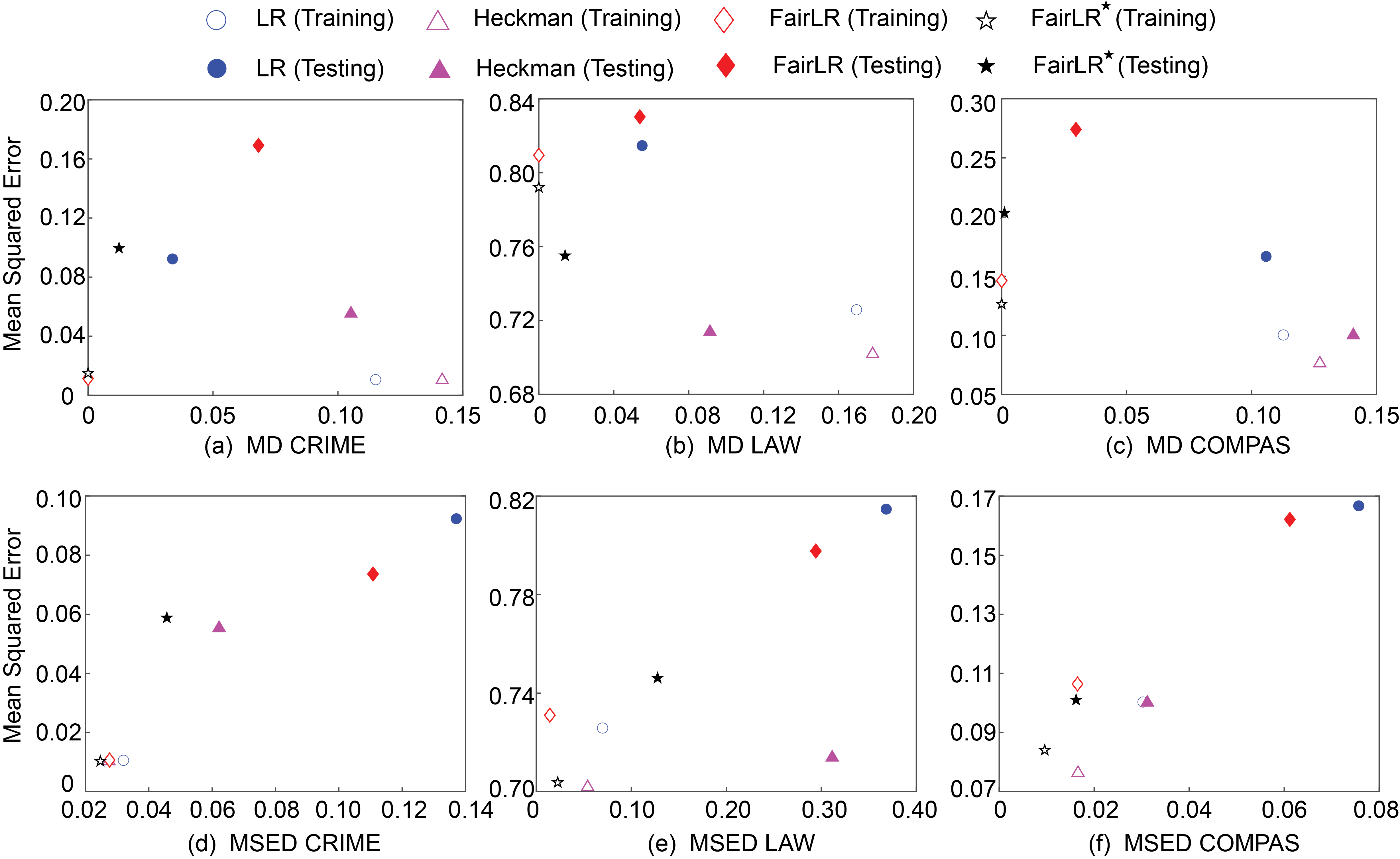
We report in Figure 2 our main comparison results on three datasets. Y-axis is MSE to reflect prediction accuracy and X-axis is based on the fairness metric chosen in fair regression models (FairLR and $\textit{FairLR}^{\star}$). In particular, the three plots in the first row of Figure 2 report MD whereas those on the second row report MSED. In each plot, we have eight markers with different shape and color, each of which reflects the MSE and fairness metric for one of the four compared models on either $\mathcal{D}_{s}$ or testing data. Throughout this section, we use $\circ$, $\triangle$, $\diamond$, and $\star$ to denote LR, Heckman, FairLR and $\textit{FairLR}^{\star}$, and use hollow (solid) marker to represent results on $\mathcal{D}_{s}$ (testing data). In general, markers in bottom-left region (close to origin) indicate good performance of corresponding methods as we want to achieve both low MSE for prediction and low MD/MSED for fairness.

We focus on the main results of comparing four methods on testing data, reflected by four solid markers in each plot ¹¹ 1 Due to space limit, we skip the comparison results of four methods on $\mathcal{D}_{s}$ reflected by four hollow markers in each plot.. We clearly see that markers of Heckman always locate below that of LR, indicating Heckman successfully corrects the sample selection bias and reduces prediction error on testing data. Taking Figure 2 (a) as an example, the MSE of Heckman is 0.0553 whereas the MSE of LR is 0.0923. Similarly, as FairLR does not do bias correction, the solid marker of FairLR is also higher than that of $\textit{FairLR}^{\star}$ for all three datasets. This demonstrates the effectiveness of Heckman model for correcting sample selection bias. Moreover, the solid marker of FairLR is always on the right side of $\textit{FairLR}^{\star}$, reflecting that FairLR simply trained on $\mathcal{D}_{s}$ without bias correction fails to achieve fairness on testing data. For example, in Figure 2 (f), the MSED of FairLR is 0.0612 whereas that of $\textit{FairLR}^{\star}$ is 0.0162. To conclude, our proposed $\textit{FairLR}^{\star}$ achieves the best trade-off between fairness and regression accuracy on the testing data.

It is also interesting to compare each model’s performance between the training data and testing data. For our $\textit{FairLR}^{\star}$, we can see its hollow marker and solid marker are close to each other horizontally, indicating that the fairness achieved on $\mathcal{D}_{s}$ can also guarantee the testing fairness. However, the hollow marker and solid marker of FairLR are separate, indicating the sample selection bias can incur unfairness in the testing data although FairLR achieved training fairness.

We conduct experiments on CRIME by using the original numerical attribute AAPR as sensitive attribute. We use Pearson coefficient to measure the independence between $\hat{Y}$ and $A$, and use Partial coefficient to measure the conditional independence of $\hat{Y}$ and $A$ given the true target value $Y$. Figure 3 shows the comparison results of four models. We have similar observations as the binary protected attribute setting. First, for results on $\mathcal{D}_{s}$ reflected by hollow markers, there is no surprise that all of the hollow markers are in bottom region with low MSE, and both FairLR and $\textit{FairLR}^{\star}$ can achieve training fairness in terms of both Pearson coefficient and Partial coefficient. Second, for results on testing data reflected by solid markers, Heckman ($\textit{FairLR}^{\star}$) achieves lower MSE than LR (FairLR) as the former model considers the sample bias selection. More importantly, only $\textit{FairLR}^{\star}$ is able to achieve testing fairness given the fairness threshold.

In this section, we evaluate how ratio $r=|\mathcal{D}_{u}|/|\mathcal{D}|$ would affect the performance of our $\textit{FairLR}^{\star}$ and baseline FairLR on the testing data. Note that larger $r$ indicates more bias in sample selection. We conduct experiments on CRIME. Figure 4 plots results of MD and MSED. In both plots, X-axis shows the varied $r$ values from 0.1 to 0.4, the left Y-axis shows MSE, and the right Y-axis shows the fairness metric (MD or MSED). Correspondingly, we use solid lines to represent MSE values and dashed lines to represent fairness values. It is unsurprising to see that $\textit{FairLR}^{\star}$ always achieves better performance (smaller MSE and smaller MD or MSED) than FairLR, as demonstrated in Figure 4 that lines with symbol $\star$ locate below those with symbol $\diamond$. More importantly, for our $\textit{FairLR}^{\star}$, the fairness value (MD or MSED) and prediction error (MSE) are stable when $r$ increases, demonstrating the robustness of our $\textit{FairLR}^{\star}$ against sample selection bias. On the contrary, for FairLR, both the unfairness and prediction error on the testing data increase when $r$ increases.

References

- [1] http://archive.ics.uci.edu/ml/datasets/communities+and+crime, 2009.
- [2] Alekh Agarwal, Alina Beygelzimer, Miroslav Dudík, John Langford, and Hanna Wallach. A reductions approach to fair classification. In International Conference on Machine Learning, pages 60–69. PMLR, 2018.
- [3] Alekh Agarwal, Miroslav Dudík, and Zhiwei Steven Wu. Fair regression: Quantitative definitions and reduction-based algorithms. In Proceedings of the 36th International Conference on Machine Learning ICML, volume 97, pages 120–129. PMLR, 2019.
- [4] Shahab Asoodeh, Fady Alajaji, and Tamás Linder. On maximal correlation, mutual information and data privacy. In 2015 IEEE 14th Canadian workshop on information theory (CWIT), pages 27–31. IEEE, 2015.
- [5] Richard Berk, Hoda Heidari, Shahin Jabbari, Matthew Joseph, Michael Kearns, Jamie Morgenstern, Seth Neel, and Aaron Roth. A convex framework for fair regression. In FAT ML, 2018.
- [6] Stephen Boyd, Stephen P Boyd, and Lieven Vandenberghe. Convex optimization. Cambridge university press, 2004.
- [7] Toon Calders, Asim Karim, Faisal Kamiran, Wasif Ali, and Xiangliang Zhang. Controlling attribute effect in linear regression. In 2013 IEEE 13th international conference on data mining, pages 71–80. IEEE, 2013.
- [8] Evgenii Chzhen, Christophe Denis, Mohamed Hebiri, Luca Oneto, and Massimiliano Pontil. Fair regression via plug-in estimator and recalibration with statistical guarantees. In Advances in Neural Information Processing Systems 33: Annual Conference on Neural Information Processing Systems 2020, NeurIPS 2020, December 6-12, 2020, virtual, 2020.
- [9] Evgenii Chzhen, Christophe Denis, Mohamed Hebiri, Luca Oneto, and Massimiliano Pontil. Fair regression with wasserstein barycenters. arXiv preprint arXiv:2006.07286, 2020.
- [10] Wei Du and Xintao Wu. Fair and robust classification under sample selection bias. In Proceedings of the 2021 ACM International Conference on Information and Knowledge Management (CIKM). ACM, 2021.
- [11] Wei Du, Depeng Xu, Xintao Wu, and Hanghang Tong. Fairness-aware agnostic federated learning. In Proceedings of the 2021 SIAM International Conference on Data Mining (SDM), pages 181–189. SIAM, 2021.
- [12] Jack Fitzsimons, AbdulRahman Al Ali, Michael Osborne, and Stephen Roberts. A general framework for fair regression. Entropy, 21(8):741, 2019.
- [13] Vincent Grari, Boris Ruf, Sylvain Lamprier, and Marcin Detyniecki. Fairness-aware neural rényi minimization for continuous features. In IJCAI, 2020.
- [14] Moritz Hardt, Eric Price, and Nati Srebro. Equality of opportunity in supervised learning. In Advances in neural information processing systems, pages 3315–3323, 2016.
- [15] James J Heckman. Sample selection bias as a specification error. Econometrica: Journal of the econometric society, pages 153–161, 1979.
- [16] Heinrich Jiang and Ofir Nachum. Identifying and correcting label bias in machine learning. In AISTATS, 2020.
- [17] Kory D Johnson, Dean P Foster, and Robert A Stine. Impartial predictive modeling: Ensuring group fairness in arbitrary models. arXiv e-prints, pages arXiv–1608, 2016.
- [18] Nathan Kallus and Angela Zhou. Residual unfairness in fair machine learning from prejudiced data. In ICML, 2018.
- [19] Jon Kleinberg, Sendhil Mullainathan, and Manish Raghavan. Inherent trade-offs in the fair determination of risk scores. arXiv preprint arXiv:1609.05807, 2016.
- [20] Junpei Komiyama, Akiko Takeda, Junya Honda, and Hajime Shimao. Nonconvex optimization for regression with fairness constraints. In International conference on machine learning, pages 2737–2746. PMLR, 2018.
- [21] Pierre Laforgue and Stephan Clémençon. Statistical learning from biased training samples. arXiv preprint arXiv:1906.12304, 2019.
- [22] J. Larson, S. Mattu, L. Kirchner, and J. Angwin. Compas dataset. https://github.com/propublica/compas-analysis, 2017.
- [23] Thibaut Le Gouic and Jean-Michel Loubes. Computing the price for fairness in a regression framework. arXiv preprint arXiv:2005.11720, 2020.
- [24] Jérémie Mary, Clément Calauzenes, and Noureddine El Karoui. Fairness-aware learning for continuous attributes and treatments. In International Conference on Machine Learning, pages 4382–4391. PMLR, 2019.
- [25] Jose G Moreno-Torres, Troy Raeder, Rocío Alaiz-Rodríguez, Nitesh V Chawla, and Francisco Herrera. A unifying view on dataset shift in classification. Pattern recognition, 45(1):521–530, 2012.
- [26] Harikrishna Narasimhan, Andrew Cotter, Maya Gupta, and Serena Wang. Pairwise fairness for ranking and regression. In Proceedings of the AAAI Conference on Artificial Intelligence, 2020.
- [27] Patrick Puhani. The heckman correction for sample selection and its critique. Journal of economic surveys, 14(1):53–68, 2000.
- [28] Ashkan Rezaei, Rizal Fathony, Omid Memarrast, and Brian D. Ziebart. Fairness for robust log loss classification. In AAAI, 2020.
- [29] Candice Schumann, Xuezhi Wang, Alex Beutel, Jilin Chen, Hai Qian, and Ed H Chi. Transfer of machine learning fairness across domains. arXiv preprint arXiv:1906.09688, 2019.
- [30] Daniel Steinberg, Alistair Reid, Simon O’Callaghan, Finnian Lattimore, Lachlan McCalman, and Tibério S. Caetano. Fast fair regression via efficient approximations of mutual information. CoRR, abs/2002.06200, 2020.
- [31] Bahar Taskesen, Viet Anh Nguyen, Daniel Kuhn, and Jose Blanchet. A distributionally robust approach to fair classification. arXiv preprint arXiv:2007.09530, 2020.
- [32] Junfeng Wen, Chun-Nam Yu, and Russell Greiner. Robust learning under uncertain test distributions: Relating covariate shift to model misspecification. In ICML, 2014.
- [33] Linda F Wightman. Lsac national longitudinal bar passage study. lsac research report series. 1998.
- [34] Chen Zhao and Feng Chen. Unfairness discovery and prevention for few-shot regression. In 2020 IEEE International Conference on Knowledge Graph (ICKG), pages 137–144. IEEE, 2020.