跳到论文正文
W Papers独立论文阅读器 arXiv:2110.04364 论文正文 计算阅读时间 · 0%
引用这篇论文根据当前论文元数据生成,正式投稿前建议核对。


License: arXiv.org perpetual non-exclusive license
arXiv:2110.04364v2 [hep-th] 08 Mar 2022

The Wilson Loop – Large Spin OPE Dictionary

Carlos Bercini1{}^{\text{\tiny 1}}, Vasco Gonçalves1,2{}^{\text{\tiny 1,\tiny 2}}, Alexandre Homrich1, 3, 4{}^{\text{\tiny 1, \tiny 3, \tiny 4}} Pedro Vieira1,3{}^{\text{\tiny 1,\tiny 3}} †† #@gmail.com&/@{carlos.bercini,vasco.dfg,alexandre.homrich,pedrogvieira}

1{}^{\text{\tiny 1}}ICTP South American Institute for Fundamental Research, IFT-UNESP, São Paulo, SP Brazil 01440-070
2{}^{\text{\tiny 2}}Centro de Fisica do Porto e Departamento de Fisica e Astronomia, Faculdade de Ciencias da Universidade do Porto, Porto 4169-007, Portugal
3{}^{\text{\tiny 3}}Perimeter Institute for Theoretical Physics, Waterloo, Ontario N2L 2Y5, Canada
4{}^{\text{\tiny 4}}Walter Burke Institute for Theoretical Physics, California Institute of Technology, Pasadena, California 91125, USA

Abstract

We work out the map between null polygonal hexagonal Wilson loops and spinning three point functions in large NN conformal gauge theories by mapping the variables describing the two different physical quantities and by working out the precise normalization factors entering this duality. By fixing all the kinematics we open the ground for a precise study of the dynamics underlying these dualities – most notably through integrability in the case of planar maximally supersymmetric Yang-Mills theory.

1 Introduction

In appendix B of [1] a duality was proposed between the nn-point correlation functions of large spin single trace twist-two operators in planar 𝒩=4\mathcal{N}=4 SYM and the expectation value of null polygonal Wilson loops with 2​n2n sides.11 1 This duality is one branch out of a rich web of dualities relating various seemingly distinct quantities in 𝒩=4\mathcal{N}=4 SYM such as Wilson Loops and Scattering Amplitudes [2] and Wilson loop and the null limit of correlation functions [3]. Indeed, null correlation functions are dominated by leading twist large spin operators which is one way to argue for the duality mentioned in the main text. The argument in [1] also uses some string theory intuition coming from the behavior of minimal surfaces of spinning strings and how they are expected to become related to the minimal surface describing null polygonal Wilson loops when their spin is taken to infinity. The argument was qualitative and no precise equality was spelled out in [1]. Our main result (23) fills in this gap. The simplest non-trivial example of such duality would relate three point functions and the null hexagon Wilson loop

(1) ⟨𝒪J1​(x1,ϵ1)​𝒪J2​(x2,ϵ2)​𝒪J3​(x3,ϵ3)⟩⟷𝕎⁡(U1,U2,U3)\langle\mathcal{O}_{J_{1}}(x_{1},\epsilon_{1})\mathcal{O}_{J_{2}}(x_{2},\epsilon_{2})\mathcal{O}_{J_{3}}(x_{3},\epsilon_{3})\rangle\longleftrightarrow\mathbb{W}(U_{1},U_{2},U_{3})

The goal of this paper is to sharpen the arrow in this relation making it into a precise equation with an equal sign with all the appropriate normalizations and with a precise dictionary relating the variables on both sides of this equation: the spins JjJ_{j} and polarization vector ϵj\epsilon_{j} on the left hand side and the hexagon cross-ratios UiU_{i} on the right hand side.

This is (23).22 2 The reader might be frowning. In (23) there are ℓi\ell_{i}’s instead of ϵi\epsilon_{i}’s. Worry not, they are simply conjugate variables as reviewed in the next section and it is straightforward to change from one to the other. The map of kinematics using the spinors is given in (38).

We got there in two steps. First we examined the OPE decomposition of six point functions in the so-called snowflake channel: we fuse adjacent pairs of external operators into spinning operators which are then glued together through a tensor structure parametrized by integer indices ℓi\ell_{i}. The starting point is intimidating. It is given by 9 sums (33 are spin sums, 33 are sums over tensor structures indices and the last 33 appear in the representation of the relevant conformal block). When the external points approach the cusps of a null hexagon, six of these sums can be performed by saddle point. The location of the saddle point will fix the tensor structure indices ℓj\ell_{j} to precise locations depending on the cross-ratios UjU_{j} of the null hexagon. This gives us the map ℓ⁡(U)\ell(U) spelled out in equation (10) below. Next we analysed further the null six point correlator through an analytic bootstrap perspective (generalizing [5] – where this was carried over for small UjU_{j} in the so called origin limit [12] – to generic finite cross-ratios UjU_{j}). This allowed us to see how the correlators becomes Wilson loops and what are all the precise conversion factors showing up along the way.

Null hexagon Wilson loops have light-cone singularities when non-adjacent vertices become null. We conjecture how these singularities emerge from the discrete structure of the structure constants in the large spin limit. The limit (1) should be understood to hold before light-cones are crossed, i.e. in the “Euclidean" region of positive cross ratios. Configurations with time-like separations should then be achieved through analytic continuation from this safe region. These musings are backed up by explorations of novel one loop data we extract.

In sum, in this paper we cleaned up the kinematics behind the duality (1) using bootstrap techniques. We are currently investigating its dynamics with integrability.

2 Spinning Three Point Functions

The purpose of this section is to establish notation. A traceless symmetric, spin JJ, primary operator in a CFT can be represented through an homogenous polynomial of degree JJ on an auxiliary null polarization vector ϵ\epsilon

(2) 𝒪J​(x,ϵ)=ϵμ1​…​ϵμJ​𝒪μ1​…​μJ​(x).\mathcal{O}_{J}(x,\epsilon)=\epsilon_{\mu_{1}}\dots\epsilon_{\mu_{J}}\mathcal{O}^{\mu_{1}\dots\mu_{J}}(x).

In a parity preserving 4D CFT, three point functions of traceless symmetric parity even operators can be parametrized as

(3) ⟨𝒪J1​(x1,ϵ1),𝒪J2​(x2,ϵ2),𝒪J3​(x3,ϵ3)⟩=∑ℓiCℓ1,ℓ2,ℓ3J1,J2,J3​V1,23J1−ℓ2−ℓ3​V2,31J2−ℓ3−ℓ1​V3,12J3−ℓ1−ℓ2​H23ℓ1​H31ℓ2​H12ℓ3(x122)κ1+κ2−κ32​(x232)κ2+κ3−κ12​(x312)κ3+κ1−κ22,\langle\mathcal{O}_{J_{1}}(x_{1},\epsilon_{1}),\mathcal{O}_{J_{2}}(x_{2},\epsilon_{2}),\mathcal{O}_{J_{3}}(x_{3},\epsilon_{3})\rangle=\frac{\sum\limits_{\ell_{i}}C^{J_{1},J_{2},J_{3}}_{\ell_{1},\ell_{2},\ell_{3}}{V_{1,23}^{J_{1}-\ell_{2}-\ell_{3}}}{V_{2,31}^{J_{2}-\ell_{3}-\ell_{1}}}{V_{3,12}^{J_{3}-\ell_{1}-\ell_{2}}}{H_{23}^{\ell_{1}}}{H_{31}^{\ell_{2}}}{H_{12}^{\ell_{3}}}}{(x_{12}^{2})^{\frac{\kappa_{1}+\kappa_{2}-\kappa_{3}}{2}}(x_{23}^{2})^{\frac{\kappa_{2}+\kappa_{3}-\kappa_{1}}{2}}(x_{31}^{2})^{\frac{\kappa_{3}+\kappa_{1}-\kappa_{2}}{2}}},

where κi\kappa_{i} is the conformal spin and

Vi,j​k=(ϵi⋅xi​k​xi​j2−ϵi⋅xi​j​xi​k2)​1xj​k2,Hi​j=ϵi⋅xi​j​ϵj⋅xi​j−12​xi​j2​ϵi⋅ϵj,V_{i,jk}=\left(\epsilon_{i}\cdot x_{ik}x_{ij}^{2}-\epsilon_{i}\cdot x_{ij}x_{ik}^{2}\right)\frac{1}{x^{2}_{jk}},\qquad H_{ij}=\epsilon_{i}\cdot x_{ij}\epsilon_{j}\cdot x_{ij}-\tfrac{1}{2}x^{2}_{ij}\epsilon_{i}\cdot\epsilon_{j},

are a basis of conformal covariant tensors [4], see appendix A. We sum over all non-negative integers ℓ\ell’s such that all exponents in (3) are non-negative.

Henceforth we will consider twist two operators in planar 𝒩=4\mathcal{N}=4 SYM at weak coupling and use the short-hand notation C∙∙∙≡CJ1,J2,J3l1,l2,l3{C}^{\bullet\bullet\bullet}\equiv C^{J_{1},J_{2},J_{3}}_{l_{1},l_{2},l_{3}} for the structure constants of three spinning operators. We also have

(4) C∙∙∙=C^∙∙∙×∏i=13Ji!2(ℓi!)2​(2​Ji)!​(Ji+ℓi−∑j=13ℓj)!⏟C∙∙∙tree level{C}^{\bullet\bullet\bullet}=\hat{C}^{\bullet\bullet\bullet}\times\underbrace{\prod_{i=1}^{3}\frac{J_{i}!^{2}}{(\ell_{i}!)^{2}\sqrt{(2J_{i})!}(J_{i}+\ell_{i}-\sum_{j=1}^{3}\ell_{j})!}}_{{C}^{\bullet\bullet\bullet}_{\text{tree level}}}

where C^∙∙∙≡C∙∙∙/Ctree level∙∙∙\hat{C}^{\bullet\bullet\bullet}\equiv{C}^{\bullet\bullet\bullet}/{C}_{\text{tree level}}^{\bullet\bullet\bullet} is given by an expansion in small ’t Hooft coupling λ\lambda and captures all loop corrections.

3 Null Correlators and the U⁡(ℓ)U(\ell) map

We consider the null polygonal limit of the six point correlator of the lightest single trace gauge invariant scalar operators as in [5]. This correlator is given by 99 cross-ratios carefully reviewed in appendix C. We will sequentially send 66 of them to zero when taking each xix_{i} to be null separated from xi+1x_{i+1} to obtain in the end a function which depends on the remaining 33 cross-ratios. More precisely, the final result will depend on the three finite cross-ratios as well as logs of the six vanishing cross-ratios. The dependence on the latter will be through a factorized universal pre-factor which we can fix. The dependence on the finite cross-ratios will be related to the renormalized Wilson loop which is theory dependent.

Figure 1: Various snow-flake OPE limits discussed in this paper. The bottom right one is the double light-like OPE explored in this section. The top right one is the more conventional Euclidian OPE used in appendix E to extract new one loop OPE data which is analysed in appendix F. We can get to both starting from the single light-like OPE on the left.

As explained in [5] we can project into leading twist (i.e. two) in the 1212, 3434 and 5656 channel in the snowflake decomposition by taking u1,u3,u5→0u_{1},u_{3},u_{5}\to 0 or x122,x342,x562→0x_{12}^{2},x_{34}^{2},x_{56}^{2}\to 0 as depicted in figure 1a. In this limit, in perturbation theory the six point function behaves as

(5) G6​(u1,u2,u3,u4,u5,u6,U1,U2,U3)→u1​u3​u5​G^6​(u2,u4,u6,U1,U2,U3)G_{6}({\color[rgb]{1,0,0}u_{1}},u_{2},{\color[rgb]{1,0,0}u_{3}},u_{4},{\color[rgb]{1,0,0}u_{5}},u_{6},U_{1},U_{2},U_{3})\to{\color[rgb]{1,0,0}u_{1}u_{3}u_{5}}\,\hat{G}_{6}(u_{2},u_{4},u_{6},U_{1},U_{2},U_{3})

The function G^6\hat{G}_{6} has no powers of u1,u3u_{1},u_{3} or u5u_{5} but it implicitly contains arbitrarily many powers of ln⁡(u1),ln⁡(u3)\ln(u_{1}),\ln(u_{3}) and ln⁡(u5)\ln(u_{5}) arising from the anomalous dimensions of the twist two operators. This function can be expanded as

(6) G6=∑J1,J2,J3∑ℓ1,ℓ2,ℓ3P^∙∙∙(J1,J2,J3,ℓ1,ℓ2,ℓ3)⏟dynamic​∫yj∈[0,1]d​y1​d​y2​d​y3​ℱ⁡(Ji,ℓi,yi,ui,Ui)⏟kinematicsG_{6}=\sum_{J_{1},J_{2},J_{3}}\sum_{\ell_{1},\ell_{2},\ell_{3}}\underbrace{\hat{P}^{\bullet\bullet\bullet}(J_{1},J_{2},J_{3},\ell_{1},\ell_{2},\ell_{3})}_{\texttt{dynamic}}\int\limits_{y_{j}\in[0,1]}dy_{1}dy_{2}dy_{3}\underbrace{\mathcal{F}(J_{i},\ell_{i},y_{i},u_{i},U_{i})}_{\texttt{kinematics}}

where P^\hat{P} is a (theory dependent) normalized product of three point functions33 3 It is given by a product of three three point functions of two scalar and one spinning operator (for the three OPE’s of the 1212, 3434 and 5656 OPE’s of the external scalar operators) and a fully spinning three point function (the intersection of the three gray lines in figure 1), (7) P^∙∙∙(J1,J2,J3,ℓ1,ℓ2,ℓ3)=C^∙∙∙(J1,J2,J3,ℓ1,ℓ2,ℓ3)C^∘∘∙(J1)C^∘∘∙(J2)C^∘∘∙(J3).\hat{P}^{\bullet\bullet\bullet}(J_{1},J_{2},J_{3},\ell_{1},\ell_{2},\ell_{3})=\hat{C}^{\bullet\bullet\bullet}(J_{1},J_{2},J_{3},\ell_{1},\ell_{2},\ell_{3})\hat{C}^{\circ\circ\bullet}(J_{1})\hat{C}^{\circ\circ\bullet}(J_{2})\hat{C}^{\circ\circ\bullet}(J_{3})\,. Here the hat C^\hat{C} stands for tree-level normalized quantity C/Ctree levelC/C_{\text{tree level}}. and ℱ{\mathcal{F}} is a (theory independent) conformal block integrand worked out in [5] and recalled in appendix D.

Series expanding the left and right hand side of relation (6) around ui,Ui=1u_{i},U_{i}=1 – corresponding to the conventional Euclidean OPE limit depicted in figure 1b – allows us to extract structure constants P^\hat{P} for the lowest spins JJ’s and polarization integers ℓ\ell’s. This data extraction using the one loop result [6] for G6G_{6} is described in appendices E, F. This one loop OPE data will be used in section 5.

In this section, we consider instead the limit u2,u4,u6→0u_{2},u_{4},u_{6}\to 0 (at fixed UjU_{j}) – known as the Lorentzian null OPE limit depicted in figure 1c – which is realized when all external points approach the cusps of a null hexagon which in turn is parametrized by the finite cross-ratios UiU_{i}. In this limit

(8) G^6​(u2,u4,u6,U1,U2,U3)→u2​u4​u6​G~6​(U1,U2,U3)\hat{G}_{6}(u_{2},u_{4},u_{6},U_{1},U_{2},U_{3})\to{\color[rgb]{1,0,0}u_{2}u_{4}u_{6}}\,\widetilde{G}_{6}(U_{1},U_{2},U_{3})

where G~\widetilde{G} is a non-trivial function of the finite UiU_{i} which still contains arbitrary powers of ln⁡(uj)\ln(u_{j}) but no powers of uju_{j} since these were by now all sent to zero. We find two important simplifications when computing the correlator (6) in this uj→0u_{j}\to 0 limit:

  • •

    The integral is dominated by large spins JjJ_{j} and large polarization integers ℓj\ell_{j}. We can thus transform

    ∑J1,J2,J3∑ℓ1,ℓ2,ℓ3→18∫0∞dJ1dJ2dJ3dℓ1dℓ2dℓ3\sum\limits_{J_{1},J_{2},J_{3}}\sum\limits_{\ell_{1},\ell_{2},\ell_{3}}\to\frac{1}{8}\int\limits_{0}^{\infty}dJ_{1}dJ_{2}dJ_{3}d\ell_{1}d\ell_{2}d\ell_{3}

    in (6) being left with nine integrals in total. (The 8=238=2^{3} comes from the fact that the spins JJ are even.)

  • •

    Six of those nine integrals can be done by saddle point.

More precisely, we find that 0=∂ln⁡ℱ/∂ℓj=∂ln⁡ℱ/∂yj0=\partial\ln\mathcal{F}/\partial\ell_{j}=\partial\ln\mathcal{F}/\partial y_{j} leads to the saddle point location

(9) y1=J2J2+J3​U2​U3U1,y2=J3J3+J1​U1​U2U3,y3=J1J1+J2​U1​U3U2\displaystyle y_{1}=\frac{J_{2}}{J_{2}+J_{3}\sqrt{\color[rgb]{0,0,1}\frac{U_{2}U_{3}}{U_{1}}}}\,,\qquad y_{2}=\frac{J_{3}}{J_{3}+J_{1}\sqrt{\color[rgb]{0,0,1}\frac{U_{1}U_{2}}{U_{3}}}}\,,\qquad y_{3}=\frac{J_{1}}{J_{1}+J_{2}\sqrt{\color[rgb]{0,0,1}\frac{U_{1}U_{3}}{U_{2}}}}

and more importantly

(10) ℓ1=J2​J3J2+J3+J1​U2U1​U3,ℓ2=J1​J3J1+J3+J2​U1U2​U3,ℓ3=J1​J2J1+J2+J3​U3U1​U2\displaystyle{\color[rgb]{1,0,1}\ell_{1}}=\frac{J_{2}J_{3}}{J_{2}+J_{3}+J_{1}\sqrt{\color[rgb]{0,0,1}\frac{U_{2}}{U_{1}U_{3}}}}\,,\qquad{\color[rgb]{1,0,1}\ell_{2}}=\frac{J_{1}J_{3}}{J_{1}+J_{3}+J_{2}\sqrt{\color[rgb]{0,0,1}\frac{U_{1}}{U_{2}U_{3}}}}\,,\qquad{\color[rgb]{1,0,1}\ell_{3}}=\frac{J_{1}J_{2}}{J_{1}+J_{2}+J_{3}\sqrt{\color[rgb]{0,0,1}\frac{U_{3}}{U_{1}U_{2}}}}\,

which nicely relate the Wilson loop cross-ratios in the right hand side of (1) with the spin and polarization integers appearing in structure constant in the left hand side of this relation. They are the sought after dictionary between these two worlds. (If Ji≫ℓi≫1J_{i}\gg\ell_{i}\gg 1 then the UiU_{i} are very small; this was the limit studied in [5].)

The saddle point evaluation leads to

G~6=\displaystyle\widetilde{G}_{6}= 4​u2​u4​u6(U1​U2​U3)12∫0∞dJ1dJ2dJ3P^∙∙∙(J1,J2,J3,ℓ1,ℓ2,ℓ3)e−J1​J2J3×u2​U2U1​U3−J2​J3J1×u4​U1U2​U3−J1​J3J2×u6​U3U1​U2\displaystyle\frac{4\color[rgb]{1,0,0}{u_{2}u_{4}u_{6}}}{({\color[rgb]{0,0,1}U_{1}U_{2}U_{3}})^{\frac{1}{2}}}\int_{0}^{\infty}dJ_{1}\,dJ_{2}\,dJ_{3}\,\hat{P}^{\bullet\bullet\bullet}(J_{1},J_{2},J_{3},\ell_{1},\ell_{2},\ell_{3})e^{-\frac{J_{1}J_{2}}{J_{3}}\times\frac{{\color[rgb]{1,0,0}u_{2}}\sqrt{{\color[rgb]{0,0,1}U_{2}}}}{\sqrt{\color[rgb]{0,0,1}U_{1}U_{3}}}-\frac{J_{2}J_{3}}{J_{1}}\times\frac{{\color[rgb]{1,0,0}u_{4}}\sqrt{\color[rgb]{0,0,1}U_{1}}}{\sqrt{\color[rgb]{0,0,1}U_{2}U_{3}}}-\frac{J_{1}J_{3}}{J_{2}}\times\frac{{\color[rgb]{1,0,0}u_{6}}\sqrt{\color[rgb]{0,0,1}U_{3}}}{\sqrt{\color[rgb]{0,0,1}U_{1}U_{2}}}}
(11) ×2γ1+γ2+γ3​(u1J1)γ12​(u3J2)γ22​(u5J3)γ32​(ℓ1U112)−γ1+γ2+γ32​(ℓ2U312)γ1−γ2+γ32​(ℓ3U212)γ1+γ2−γ32,\displaystyle\times 2^{\gamma_{1}+\gamma_{2}+\gamma_{3}}\left(\frac{{\color[rgb]{1,0,0}u_{1}}}{J_{1}}\right)^{\frac{\gamma_{1}}{2}}\left(\frac{{\color[rgb]{1,0,0}u_{3}}}{J_{2}}\right)^{\frac{\gamma_{2}}{2}}\left(\frac{{\color[rgb]{1,0,0}u_{5}}}{J_{3}}\right)^{\frac{\gamma_{3}}{2}}\left(\frac{\ell_{1}}{{\color[rgb]{0,0,1}U_{1}}^{\frac{1}{2}}}\right)^{\frac{-\gamma_{1}+\gamma_{2}+\gamma_{3}}{2}}\left(\frac{\ell_{2}}{{\color[rgb]{0,0,1}U_{3}}^{\frac{1}{2}}}\right)^{\frac{\gamma_{1}-\gamma_{2}+\gamma_{3}}{2}}\left(\frac{\ell_{3}}{{\color[rgb]{0,0,1}U_{2}}^{\frac{1}{2}}}\right)^{\frac{\gamma_{1}+\gamma_{2}-\gamma_{3}}{2}},

where ℓj\ell_{j} depend on the integration variables JjJ_{j} through (10). Implicit in this discussion is the assumption that the integral is dominated by the saddle point developed by the conformal block integrand. This should be valid for positive UUs, see further discussion in section 5. One can nicely check that when λ=0\lambda=0 (so that the full second line as well as P^∙∙∙\hat{P}^{\bullet\bullet\bullet} can be set to 1) this expression indeed integrates into the free theory result G~6=1\widetilde{G}_{6}=1.

We close this section with the inverse of the map (10):

U1=J1​J3​ℓ1​ℓ3((J2+J3)​ℓ1−J2​J3)​((J1+J2)​ℓ3−J1​J2),\displaystyle{\color[rgb]{0,0,1}U_{1}}=\frac{J_{1}J_{3}{\color[rgb]{1,0,1}\ell_{1}\ell_{3}}}{\left(\left(J_{2}+J_{3}\right){\color[rgb]{1,0,1}\ell_{1}}-J_{2}J_{3}\right)\left(\left(J_{1}+J_{2}\right){\color[rgb]{1,0,1}\ell_{3}}-J_{1}J_{2}\right)}\,,
U2=J2​J3​ℓ2​ℓ3((J1+J3)​ℓ2−J1​J3)​((J1+J2)​ℓ3−J1​J2),\displaystyle{\color[rgb]{0,0,1}U_{2}}=\frac{J_{2}J_{3}{\color[rgb]{1,0,1}\ell_{2}\ell_{3}}}{\left(\left(J_{1}+J_{3}\right){\color[rgb]{1,0,1}\ell_{2}}-J_{1}J_{3}\right)\left(\left(J_{1}+J_{2}\right){\color[rgb]{1,0,1}\ell_{3}}-J_{1}J_{2}\right)}\,,
(12) U3=J1​J2​ℓ1​ℓ2((J2+J3)​ℓ1−J2​J3)​((J1+J3)​ℓ2−J1​J3).\displaystyle{\color[rgb]{0,0,1}U_{3}}=\frac{J_{1}J_{2}{\color[rgb]{1,0,1}\ell_{1}\ell_{2}}}{\left(\left(J_{2}+J_{3}\right){\color[rgb]{1,0,1}\ell_{1}}-J_{2}J_{3}\right)\left(\left(J_{1}+J_{3}\right){\color[rgb]{1,0,1}\ell_{2}}-J_{1}J_{3}\right)}\,.

It is going to be used intensively below.

4 Multi-point Null Bootstrap and the C123/𝕎C_{123}/\mathbb{W} relation

We took a limit where all points approach the boundary of a null hexagon corresponding to all uj→0u_{j}\to 0. Because we did it in two steps (first u1,u3,u5→0u_{1},u_{3},u_{5}\to 0 projecting to leading twist and then u2,u4,u6→0u_{2},u_{4},u_{6}\to 0 projecting to large spin) the final result (11) is not manifestly cyclic invariant. In this section we follow [5] and impose the cyclic symmetry of our correlator under ui→ui+1u_{i}\to u_{i+1} and Ui→Ui+1U_{i}\to U_{i+1} to further constraint the structure constants P^\hat{P}. This will generalize the result in [5] from the origin kinematics to generic hexagon cross-ratios.

To kick this analysis off we start by converting the starting point (11) from the cross-ratios uju_{j} to the more local cross-ratios vjv_{j} (both are reviewed in appendix C) since the expectation is that the Wilson loop should factorize into a universal prefactor depending on these variables alone times a renormalized Wilson loop [3, 5]. Beautifully, we see that this factorization is almost automatic once we convert to the vv variables. Indeed, we find

G~6=\displaystyle\widetilde{G}_{6}=  4​v2​v4​v6​∫0∞d​J1​d​J2​d​J3​e−J1​J2J3​v2​v6v4−J2​J3J1​v2​v4v6−J1​J3J2​v4​v6v2+γ14​ln⁡16​v1​v5v3​J12+γ24​ln⁡16​v1​v3v5​J22+γ34​ln⁡16​v3​v5v1​J32\displaystyle\,4\,\sqrt{v_{2}v_{4}v_{6}}\hskip 2.0pt\!\int\limits_{0}^{\infty}\!dJ_{1}\,dJ_{2}\,dJ_{3}\,e^{-\frac{J_{1}J_{2}}{J_{3}}\,\sqrt{\frac{v_{2}v_{6}}{v_{4}}}-\frac{J_{2}J_{3}}{J_{1}}\,\sqrt{\frac{v_{2}v_{4}}{v_{6}}}-\frac{J_{1}J_{3}}{J_{2}}\,\sqrt{\frac{v_{4}v_{6}}{v_{2}}}+\frac{\gamma_{1}}{4}\ln\frac{16v_{1}v_{5}}{v_{3}J_{1}^{2}}+\frac{\gamma_{2}}{4}\ln\frac{16v_{1}v_{3}}{v_{5}J_{2}^{2}}+\frac{\gamma_{3}}{4}\ln\frac{16v_{3}v_{5}}{v_{1}J_{3}^{2}}}
(13) ×P^∙∙∙(J1,J2,J3,ℓ1,ℓ2,ℓ3)/∏i=13ℓiγi−γi+1−γi−12\displaystyle\,\times\hat{P}^{\bullet\bullet\bullet}(J_{1},J_{2},J_{3},\ell_{1},\ell_{2},\ell_{3})/\prod_{i=1}^{3}\ell_{i}^{\frac{\gamma_{i}-\gamma_{i+1}-\gamma_{i-1}}{2}}

so that the first line is already only made out of vjv_{j}’s while all UjU_{j} dependence arises from the second line through the ℓj​(Ji,Ui)\ell_{j}(J_{i},U_{i}) map (10). The problem at this point is how to constrain P^\hat{P} so that the UjU_{j} and vjv_{j} dependence factorizes and so that the final result is cyclic invariant under vj,Uj→vj+1,Uj+1v_{j},U_{j}\to v_{j+1},U_{j+1}. The factorization would be automatic as soon as the ℓj\ell_{j} dependence in P^\hat{P} comes through a factor of the form

(14) factor≡∏i=13ℓiγi−γi+1−γi−12×\displaystyle\texttt{factor}\equiv\prod_{i=1}^{3}{\color[rgb]{1,0,1}\ell_{i}}^{\frac{\gamma_{i}-\gamma_{i+1}-\gamma_{i-1}}{2}}\,\times
×𝕎⁡(J1​J3​ℓ1​ℓ3((J2+J3)​ℓ1−J2​J3)​((J1+J2)​ℓ3−J1​J2),J1​J3​ℓ1​ℓ3((J2+J3)​ℓ1−J2​J3)​((J1+J2)​ℓ3−J1​J2),J1​J3​ℓ1​ℓ3((J2+J3)​ℓ1−J2​J3)​((J1+J2)​ℓ3−J1​J2))\displaystyle\times\mathbb{W}(\tfrac{J_{1}J_{3}{\color[rgb]{1,0,1}\ell_{1}\ell_{3}}}{\left(\left(J_{2}+J_{3}\right){\color[rgb]{1,0,1}\ell_{1}}-J_{2}J_{3}\right)\left(\left(J_{1}+J_{2}\right){\color[rgb]{1,0,1}\ell_{3}}-J_{1}J_{2}\right)},\tfrac{J_{1}J_{3}{\color[rgb]{1,0,1}\ell_{1}\ell_{3}}}{\left(\left(J_{2}+J_{3}\right){\color[rgb]{1,0,1}\ell_{1}}-J_{2}J_{3}\right)\left(\left(J_{1}+J_{2}\right){\color[rgb]{1,0,1}\ell_{3}}-J_{1}J_{2}\right)},\tfrac{J_{1}J_{3}{\color[rgb]{1,0,1}\ell_{1}\ell_{3}}}{\left(\left(J_{2}+J_{3}\right){\color[rgb]{1,0,1}\ell_{1}}-J_{2}J_{3}\right)\left(\left(J_{1}+J_{2}\right){\color[rgb]{1,0,1}\ell_{3}}-J_{1}J_{2}\right)})\,

Indeed, the first factor would cancel precisely the factor in the denominator in the last line of (13) whereas – on the saddle point solution (10) – the arguments of the second function will become precise the UjU_{j} variables as indicated in (12). That is, if

(15) P^∙∙∙(J1,J2,J3,ℓ1,ℓ2,ℓ3)=factor×p(J1,J2,J3).\hat{P}^{\bullet\bullet\bullet}(J_{1},J_{2},J_{3},\ell_{1},\ell_{2},\ell_{3})=\texttt{factor}\times p(J_{1},J_{2},J_{3})\,.

then we automatically find an explicit factorization

(16) G~6=\displaystyle\widetilde{G}_{6}= 𝕎(U1,U2,U3)×[ 4v2​v4​v6∫0∞dJ1dJ2dJ3e−J1​J2J3​v2​v6v4−J2​J3J1​v2​v4v6−J1​J3J2​v4​v6v2\displaystyle\mathbb{W}(U_{1},U_{2},U_{3})\times\Big[\,4\sqrt{v_{2}v_{4}v_{6}}\hskip 2.0pt\!\int\limits_{0}^{\infty}\!dJ_{1}\,dJ_{2}\,dJ_{3}\,e^{-\frac{J_{1}J_{2}}{J_{3}}\,\sqrt{\frac{v_{2}v_{6}}{v_{4}}}-\frac{J_{2}J_{3}}{J_{1}}\,\sqrt{\frac{v_{2}v_{4}}{v_{6}}}-\frac{J_{1}J_{3}}{J_{2}}\,\sqrt{\frac{v_{4}v_{6}}{v_{2}}}}
ef4​ln⁡(J1)​ln⁡(v1​v5v3)+f4​ln⁡(J2)​ln⁡(v1​v3v5)+f4​ln⁡(J3)​ln⁡(v3​v5v1)+g4​ln⁡(163​v1​v3​v5J12​J22​J32)−f2​∑j=13ln⁡(Jj)​ln⁡(Jj/4)p(J1,J2,J3)]\displaystyle\!\!\!\!\!e^{\frac{f}{4}\ln(J_{1})\ln\!\big(\!\frac{v_{1}v_{5}}{v_{3}}\!\big)+\frac{f}{4}\ln(J_{2})\ln\!\big(\!\frac{v_{1}v_{3}}{v_{5}}\!\big)+\frac{f}{4}\ln(J_{3})\ln\!\big(\!\frac{v_{3}v_{5}}{v_{1}}\!\big)+\frac{g}{4}\ln\!\big(\!\frac{16^{3}v_{1}v_{3}v_{5}}{J_{1}^{2}J_{2}^{2}J_{3}^{2}}\!\big)-\frac{f}{2}\sum\limits_{j=1}^{3}\ln(J_{j})\ln(J_{j}/4)}p(J_{1},J_{2},J_{3})\Big]

where we have used the explicit form of the large spin anomalous dimension γi=f​ln⁡(Ji)+g\gamma_{i}=f\ln(J_{i})+g to massage the second line. It is hard to imagine how anything else would lead to a factorization but we did not establish the uniqueness of (15); it is a conjecture which passes some non-trivial checks below and reduces to [5] in the origin limit.44 4 The challenge is to relate (non-)factorization of integrands versus (non-)factorization of integrated expressions. Any extra ℓj\ell_{j} dependence in (15) would show up inside the square bracket in (16) and thus generically lead to a UjU_{j} dependence once we integrate in JjJ_{j} with (10). It might be that a very subtle ℓj\ell_{j} dependence could integrate to zero or generate a factorized function of UjU_{j} which would renormalize 𝕎\mathbb{W}. We were not imaginative enough to find any such example which made us confident that (15) is indeed unique.

Next we have to impose cyclicity. For the first factor in (16) this simply means that 𝕎⁡(U1,U2,U3)=𝕎⁡(U2,U3,U1)\mathbb{W}(U_{1},U_{2},U_{3})=\mathbb{W}(U_{2},U_{3},U_{1}) but it does not constraint 𝕎\mathbb{W} any further. On the contrary, for the second factor, cyclicity is very powerful. It fixes pp completely to all loop orders in perturbation theory, under very mild assumptions as explained below. The result is remarkably simple:

(17) p⁡(J1,J2,J3)=𝒩​∏i=13(Γ⁡(1−γi)​ef2​ln⁡(Ji)2−f​ln⁡2​ln​Ji).p(J_{1},J_{2},J_{3})=\mathcal{N}\prod_{i=1}^{3}\left(\Gamma\left(1-\gamma_{i}\right)e^{\frac{f}{2}\ln(J_{i})^{2}-f\ln 2\ln J_{i}}\right).

It is a nice and very instructive exercise to plug this proposal into (16), expand the integrand to any desired order in perturbation theory (corresponding to small cusp anomalous dimension ff and small collinear anomalous dimension gg), perform all the resulting integrations and realize that we only generate ln⁡(vj)\ln(v_{j})’s and that moreover the result non-trivially combines, order by order in perturbation theory, into a fully cyclic expression.

It is an even more instructive exercise to simply plug a general perturbative ansatz for p⁡(J1,J2,J3)p(J_{1},J_{2},J_{3}) as an infinite series of monomials made out of powers of ln⁡(Ji)\ln(J_{i})’s in (16). Each such monomial will again integrate to simple polynomials in ln⁡(vj)\ln(v_{j})’s. Remarkably, imposing cyclicity at each order of perturbation theory will completely fix these polynomials and thus the full perturbative expansion up to an overall normalization constant. In this way, by considering a very large number of loops we could eventually recognize a simple pattern and arrive at (17). This brute force derivation is perfectly valid but was not how we originally arrived at (17).

We proceeded in a slightly more sophisticated way following similar ideas in the four point function analysis in [7]. This is explained in the box that follows; this discussion can be probably skipped in a first reading.

We first look for an integral transform for pp such that ciclicity can be imposed at integrand level. We define (18) q(lnJ1,lnJ2,lnJ3)=e−f2∑j=13ln(Jj)ln(Jj/4)p(J1,J2,J3)q\,(\ln J_{1},\ln J_{2},\ln J_{3})=e^{-\frac{f}{2}\sum\limits_{j=1}^{3}\ln(J_{j})\ln(J_{j}/4)}p(J_{1},J_{2},J_{3}) to absorb the last factor in the exponential in the second line in (16) and we change integration variables to (19) x1=J2​J3J1​v2​v4v6,x3=J1​J2J3​v2​v6v4,x5=J1​J3J2​v4​v6v2,x_{1}=\frac{J_{2}J_{3}}{J_{1}}\sqrt{\frac{v_{2}v_{4}}{v_{6}}},\hskip 17.00024ptx_{3}=\frac{J_{1}J_{2}}{J_{3}}\sqrt{\frac{v_{2}v_{6}}{v_{4}}},\hskip 17.00024ptx_{5}=\frac{J_{1}J_{3}}{J_{2}}\sqrt{\frac{v_{4}v_{6}}{v_{2}}},\hskip 17.00024pt to trivialize the tree level measure. Then the previous expression (16) takes the very suggestive form (20) G~6=\displaystyle\widetilde{G}_{6}= 𝕎(U1,U2,U3)×e∑if16​ln​vi​ln​vi+3−f8​ln​vi​ln​vi+1+g4​ln​vi×\displaystyle\mathbb{W}(U_{1},U_{2},U_{3})\times e^{\sum\limits_{i}\frac{f}{16}\ln v_{i}\ln v_{i+3}-\frac{f}{8}\ln v_{i}\ln v_{i+1}+\frac{g}{4}\ln v_{i}}\times ×∫0∞dx1dx3dx5e−∑i=13(x2​i−1+g2ln(x2​i−1/4)−f4ln(x2​i−1)ln(v2​i−1))\displaystyle\times\int\limits_{0}^{\infty}dx_{1}\,dx_{3}\,dx_{5}\,e^{-\sum\limits_{i=1}^{3}(x_{2i-1}+\frac{g}{2}\ln(x_{2i-1}/4)-\frac{f}{4}\ln(x_{2i-1})\ln(v_{2i-1}))} ×q⁡(ln⁡x1+ln⁡x5−ln⁡v62,ln⁡x3+ln⁡x1−ln⁡v22,ln⁡x3+ln⁡x5−ln⁡v42)\displaystyle\hskip 17.00024pt\hskip 17.00024pt\times q\left(\frac{\ln x_{1}+\ln x_{5}-\ln v_{6}}{2},\frac{\ln x_{3}+\ln x_{1}-\ln v_{2}}{2},\frac{\ln x_{3}+\ln x_{5}-\ln v_{4}}{2}\right) where we see the explicit appearance of the Sudakov factor [3, 5] in the first line. The lack of ciclicity is now quite striking in the very different way that the even and odd cross-ratios show up in the integral: The odd cross-ratios appear in the exponent in the form ln⁡(xi)​ln⁡(vi)\ln(x_{i})\ln(v_{i}) while the even cross-ratios appear inside the arguments of the dressed structure constant p^\hat{p}. That asymmetry is trivial to fix: It suffices to write qq itself as an integral transform introducing three new integration variables x2,x4,x6x_{2},x_{4},x_{6} as (21) q(X,Y,Z)=∫0∞dx2dx4dx6e−∑i=13(x2​i+g2ln(x2​i/4))−f2(ln(x6)X+ln(x2)Y+ln(x4)Z)q~(x4,x5,x6)\displaystyle q(X,Y,Z)=\int\limits_{0}^{\infty}dx_{2}\,dx_{4}\,dx_{6}\,e^{-\sum\limits_{i=1}^{3}(x_{2i}+\frac{g}{2}\ln(x_{2i}/4))-\frac{f}{2}(\ln(x_{6})X+\ln(x_{2})Y+\ln(x_{4})Z)}\tilde{q}(x_{4},x_{5},x_{6}) where the measure (first factor in the exponent) is written to mimic the already existing measure over x1,x3,x5x_{1},x_{3},x_{5} to make sure the full result is properly symmetric. Similarly, the factor f/2f/2 in the second factor in the exponential guarantees that the new ln⁡(xi)​ln⁡(vi)\ln(x_{i})\ln(v_{i}) terms containing the even cross-ratios come with the same overall prefactor as their odd cousins in (20). Note also that ln⁡(x6)\ln(x_{6}) will multiply XX which contains its two neighbors ln⁡(x1=6+1)\ln(x_{1=6+1}) and ln⁡(x5=6−1)\ln(x_{5=6-1}) and similarly for all other arguments. So in total we will get a beautiful symmetric chain of interactions and overall the only symmetry breaking term is q~​(x4,x5,x6)\tilde{q}(x_{4},x_{5},x_{6})! We should thus set it to a constant. Integrating (21) with q~\tilde{q} equal to a constant indeed leads to the anticipated simple result (17). This concludes our derivation.

Putting everything together we thus find the final result for the full correlator in the light-like limit (and for general hexagon kinematics) as

(22) G~6=\displaystyle\widetilde{G}_{6}= (𝕎⁡(U1,U2,U3)CLOSE⏟Renormalized Wilson loop×exp⁡(∑if16​ln​vi​ln​vi+3−f8​ln​vi​ln​vi+1+g−f​γE4​ln​vi)⏟Sudokov Factor×\displaystyle\underbrace{{\color[rgb]{1,1,1}\!\!\!\!\Big(}\mathbb{W}(U_{1},U_{2},U_{3})}_{\texttt{Renormalized Wilson loop}}\times\underbrace{\exp\big(\sum\limits_{i}\frac{f}{16}\ln v_{i}\ln v_{i+3}-\frac{f}{8}\ln v_{i}\ln v_{i+1}+{{\frac{g-f\gamma_{E}}{4}\ln v_{i}}}\big)}_{\texttt{Sudokov Factor}}\times
×𝒩(∫0∞∏j=16dxje−∑i=16(xi+g2𝐥𝐧(xi)−f4𝐥𝐧(xi)𝐥𝐧(xi+1)−f4𝐥𝐧(xi)𝐥𝐧(vi))+∑if​γE4𝐥𝐧(vi))⏟Recoil ​J,\displaystyle\times\underbrace{\mathcal{N}\left(\int\limits_{0}^{\infty}\prod_{j=1}^{6}dx_{j}e^{-\sum\limits_{i=1}^{6}(x_{i}+\frac{g}{2}\mathbf{ln}(x_{i})-\frac{f}{4}\mathbf{ln}(x_{i})\mathbf{ln}(x_{i+1})-\frac{f}{4}\mathbf{ln}(x_{i})\mathbf{ln}(v_{i}))+\sum\limits_{i}\frac{f\gamma_{E}}{4}\mathbf{ln}(v_{i})}\right)}_{\texttt{Recoil }J},

where 𝐥𝐧⁡(x)=ln⁡(x)+γE\mathbf{ln}(x)=\ln(x)+\gamma_{E}.

To obtain the full map between spinning three point functions and the Wilson loop we simply need to convert P^\hat{P} to C^\hat{C} using (7). In other words, we divide the result whence obtained by three large spin structure constants for a single spinning operator which were computed in [8]. This ratio nicely removes some of the gamma functions in (17) leading to our final main result

(23) C^∙∙∙(Ji,ℓi)=𝒩​∏i=13(Ji​ℓi2​ℓi+1​ℓi−1)γi2⏟conversion factor×𝕎(U1,U2,U3).\hat{C}^{\bullet\bullet\bullet}(J_{i},\ell_{i})=\underbrace{\mathcal{N}\prod_{i=1}^{3}\Big(\frac{J_{i}\ell_{i}}{2\ell_{i+1}\ell_{i-1}}\Big)^{\frac{\gamma_{i}}{2}}}_{\texttt{conversion factor}}\times\mathbb{W}(U_{1},U_{2},U_{3}). with the map between variables on both sides of this equation given by (10) or (12).

5 One-loop check and some speculative musings

The structure constant variables (J1,J2,J3,ℓ1,ℓ2,ℓ3)(J_{1},J_{2},J_{3},\ell_{1},\ell_{2},\ell_{3}) are mapped into the Wilson loop cross-ratios (U1,U2,U3)(U_{1},U_{2},U_{3}) through the map (12). The JiJ_{i} are even non-negative integers and the ℓi\ell_{i} are non-negative integers bounded by the condition that ℓi+ℓj≤Jk\ell_{i}+\ell_{j}\leq J_{k} with i,j,ki,j,k all different. For J1=J2=J3=30J_{1}=J_{2}=J_{3}=30 for instance we would have 78167816 discrete ℓj\ell_{j} choices, each with its own structure constant. The map (12) maps each one of these ℓj\ell_{j} choices to a point in the cross-ratio space as depicted in figure 2.

The set of ℓk<Ji​Jj/(Ji+Jj)\ell_{k}<J_{i}J_{j}/(J_{i}+J_{j}) covers the full space of positive real cross-ratios UjU_{j} as represented in the figure 2 by the blue dots/region. The remaining ℓk\ell_{k}’s cover three disjoint regions in cross-ratio space where one cross-ratio is positive and two are negative. (In the large spin limit of course.) The region of all positive cross-ratios can be called the space-like region since it can be realized with all squared distances positive. The other three regions need some squared distances to be negative to get negative cross-ratios so we call them time-like regions. (A beautiful detailed analysis of the geometry of the UiU_{i} space for hexagonal Wilson loops is given in [9].)

Refer to caption
Figure 2: The OPE data C^∙∙∙(J1,J2,J3,ℓ1,ℓ2,ℓ3)\hat{C}^{\bullet\bullet\bullet}(J_{1},J_{2},J_{3},\ell_{1},\ell_{2},\ell_{3}) can be plotted in the cross-ratio space (U1,U2,U3)(U_{1},U_{2},U_{3}) if we map the ℓi\ell_{i} and JiJ_{i} variables to the UiU_{i} using (12). The one loop structure constants have a good Ji→∞J_{i}\to\infty limit in the blue region perfectly matching with the Wilson loop in the Euclidean space-like (S)(S) sheet. In contrast, the same structure constants blow up as Ji→∞J_{i}\to\infty in the red region which would naively correspond to the Wilson loop in some Lorentzian time-like regions (Ti)(T_{i}). To reach these regions we should instead start in the blue region and take the large spin limit so that an emergent analytic structure arises with new branch cuts. We can then cross them by analytically continuing away from the blue region and in this way obtain a match beyond the Euclidean regime. The structure constant/Wilson loop duality is a cute concrete example where expansions and analytic continuations do not commute.

We propose that as we take the large Jk,ℓkJ_{k},\ell_{k} limit the structure constants in the space-like region (SS) will nicely match – according to (23) – with the Wilson loop in the space-like (or Euclidean) sheet, where we start with all cusps space-like separated and do not cross any light-cone. Let us discuss a non-trivial one loop check of this proposal.

In perturbation theory we have C^∙∙∙(Ji,ℓi)=1+λc+…\hat{C}^{\bullet\bullet\bullet}(J_{i},\ell_{i})=1+\lambda c+\dots, conversion factor=1+λ​h+…\texttt{conversion factor}=1+\lambda h+\dots and 𝕎⁡(Ui)=1+λ​w+…\mathbb{W}(U_{i})=1+\lambda w+\dots so that at one loop our prediction (23) simply translates into (up to an overall shift by a constant)

(24) c⁡(Ji,ℓi)−h⁡(Ji,ℓi)=w⁡(Ui​(Ji,ℓi)).c(J_{i},\ell_{i})-h(J_{i},\ell_{i})=w\big(U_{i}(J_{i},\ell_{i})\big)\,.

The one loop Wilson loop is universal in any non-abelian gauge theory in the planar limit since it is given by a single gluon exchange from an edge of the hexagon to another. It reads [9, 10, 11, 12]

(25) w⁡(U1,U2,U3)=−4​π2+2​∑i=13Li2​(1−1/Ui).w\big(U_{1},U_{2},U_{3}\big)=-4\pi^{2}+2\sum_{i=1}^{3}\text{Li}_{2}\left(1-1/U_{i}\right).

This object – in the space-like region where all UiU_{i} are positive – should emerge from the one loop structure constant of large spin operators. These are extracted from the OPE of the one loop correlation functions of six 20′20^{\prime} operators in planar 𝒩=4\mathcal{N}=4 SYM, see appendix E.1.

Before discussing the quantitative match of the structure constant and the Wilson loop we will open a speculative parentheses here. It can be skipped by the more orthodox readers. Note that the analytic structure of the structure constant before taking the large spin and large polarizations limit is strikingly different to that of the Wilson loop. The Wilson loop has a rich cut structure. In the physical sheet there are cuts at Ui=0U_{i}=0 which need to be crossed to go from space-like to time-like configurations. These are the only singularities of the Wilson loop in the physical space-like sheet [11]. If we cross the Ui=0U_{i}=0 cuts we go to other sheets and do see other singularities most notably at Ui=1U_{i}=1 but also at various other interesting locations, see e.g. [13]. Instead, the structure constant are meromorphic functions of ℓi\ell_{i} and JjJ_{j} with no cuts whatsoever – see appendix F.3 for explicit expressions full of Harmonic numbers, rational binomial sums and other similar meromorphic building blocks. They have poles at unphysical values of polarizations and spins. In the large ℓi\ell_{i} and JiJ_{i} limit these poles condense; seen from far away they become cuts as illustrated in figure 3. (This phenomenon of poles condensing into cuts is all over, most notably in Matrix model studies.) In other words, at finite ℓi,Ji\ell_{i},J_{i} there are no other sheets and no monodromies to be picked, only the space-like sheet exists. All other Lorentzian sheets are emergent. They only appear in the semi-classical limit of large ℓi,Ji\ell_{i},J_{i}. As such, what we expect is that if we stay in the Euclidean regime ℓk<Ji​Jj/(Ji+Jj)\ell_{k}<J_{i}J_{j}/(J_{i}+J_{j}) corresponding to the blue region in figure 2 we should obtain a match with the Wilson loop in the large spin limit. But if we want to access other regions in the Wilson loop, the order of limits is key: We first need to take the large spin and large polarization limit so cuts emerge; then we analytically continue our structure constant through those cuts. When doing a numerical comparison of the Wilson loop and the structure constants we observe an interesting phenomenon which seems to back this up. In the space-like ℓk<Ji​Jj/(Ji+Jj)\ell_{k}<J_{i}J_{j}/(J_{i}+J_{j}) region the one loop structure constants cc are O⁡(1)O(1) numbers; as we increase the spin we observe that these numbers do approach the expected Wilson loop expression (25). On the other hand, for ℓk>Ji​Jj/(Ji+Jj)\ell_{k}>J_{i}J_{j}/(J_{i}+J_{j}) the structure constants cc become exponentially large real numbers which blow up as Jj→∞J_{j}\to\infty! This is in perfect synthony with the picture of the previous paragraph: to cross the cuts and reach the Lorentzian domain -encountering a complex valued finite Wilson loop - we must first go to a safe region in the physical sheet and then take a classical limit so the cuts appear in the first place. If we go to the cuts directly in the structure constant side we encounter instead a divergence – we could call it a firewall in analogy with black holes. In this black hole analogy, the smooth cuts with emerge in the classical limit resemble the smooth black hole horizons while the poles in the structure constants which we would only see through very sensitive experiments would be the analogue of the quantum black hole micro-states inner structure; some kind of fuzzball. A analytical toy model for this phenomenon is C^∙∙∘\hat{C}^{\bullet\bullet\circ} in the large spin limit, discussed in detail in appendix F.2. In equation (63) we obtain nice O⁡(1)O(1) expressions valid for ℓ<J1​J2/(J1+J2)\ell<J_{1}J_{2}/(J_{1}+J_{2}) with emergent branch points at ℓ=J1​J2/(J1+J2)\ell=J_{1}J_{2}/(J_{1}+J_{2}) which should be thought of as analogues for the U=0U=0 light-cone singularities of the hexagonal Wilson loop. On the other hand, for ℓ>J1​J2/(J1+J2)\ell>J_{1}J_{2}/(J_{1}+J_{2}) the one-loop corrections become exponentially divergent, see equation (F.2). In fact, extending the black hole analogy, one must be careful when using these limits to compute observables that probe the “horizon" or “interior" regions. For example, the equal spins sum over ℓ\ell of the three point function is finite in the large spin limit – given by (66) in the appendix – but it is not purely captured by the naive large ℓ\ell, JJ limit with ℓ/J\ell/J fixed. Indeed, if one first takes the large spin limit, a non integrable expression is obtained in the “interior" region. This singularity can be thought of as a “UV" divergence that is regulated by finer corrections coming from the microscopical structure of three point functions. End of speculative detour.
Refer to caption
Figure 3: a) (Imaginary part of) H⁡(z)H(z) where H⁡(z)H(z) are Harmonic numbers evaluate to rational numbers for zz positive integer and has poles at negative integers. For large argument it behaves as log⁡(z)\log(z). In other words, seen from far away the poles condense into a cut. b) (Imaginary part of) log⁡(z)\log(z) lives in an infinite sheeted surface. The first one agrees with that of H⁡(z)H(z) for large arguments while the other sheets are emergent.

We could not completely fix the analytic form of the one loop structure constants c⁡(Ji,ℓi)c(J_{i},\ell_{i}) and so we could not establish (24) fully. Instead we expanded the Wilson loop around the so-called origin limit [12] corresponding to small cross-ratios. Note that we have

(26) w⁡(U1,U2,U3)=∑i=13ln2⁡(Ui)+∑i=13ln⁡(Ui)​𝒜i+ℬw\big(U_{1},U_{2},U_{3}\big)=\sum_{i=1}^{3}\ln^{2}\left(U_{i}\right)+\sum_{i=1}^{3}\ln\left(U_{i}\right)\mathcal{A}_{i}+\mathcal{B}

where 𝒜i\mathcal{A}_{i} and ℬ\mathcal{B} have regular Taylor expansions around the origin U1=U2=U3=0U_{1}=U_{2}=U_{3}=0.55 5 Explicitly, 𝒜i=2​ln⁡(1−Ui)\mathcal{A}_{i}=2\ln(1-U_{i}) and ℬ=2​Li2​(U1)+2​Li2​(U2)+2​Li2​(U3)−5​π2\mathcal{B}=2\text{Li}_{2}(U_{1})+2\text{Li}_{2}(U_{2})+2\text{Li}_{2}(U_{3})-5\pi^{2}. For instance

(27) ℬ=−5​π2+21​∑iUi+24​∑iUi2+29​∑iUi3+216​∑iUi4+…\mathcal{B}=-5\pi^{2}+\frac{2}{1}\sum_{i}U_{i}+\frac{2}{4}\sum_{i}U_{i}^{2}+\frac{2}{9}\sum_{i}U_{i}^{3}+\frac{2}{16}\sum_{i}U_{i}^{4}+\dots

The representation (26) makes manifest the branch-cuts at Ui=0U_{i}=0 of the Wilson loop. In the structure constant side, to make contact with the Wilson loop as an expansion around the origin we should consider the limit of very large spin and polarizations but very small ratios of the two,

(28) ℓi≫1,Ji≫1,ℓi/Jj≪1,\ell_{i}\gg 1\,,\qquad J_{i}\gg 1\,,\qquad\ell_{i}/J_{j}\ll 1\,,

indeed, in this regime we easily see that the cross-ratios obtained through (12) are very small, for example:

(29) U1=ℓ1​ℓ3J22+ℓ12​ℓ3J23+ℓ12​ℓ3J22​J3+ℓ1​ℓ32J23+ℓ1​ℓ32J1​J22+…,ln⁡(U1)=ln⁡(ℓ1​ℓ3J22)+ℓ1J2+ℓ1J3+ℓ3J1+ℓ3J2+….U_{1}=\frac{\ell_{1}\ell_{3}}{J_{2}^{2}}+\frac{\ell_{1}^{2}\ell_{3}}{J_{2}^{3}}+\frac{\ell_{1}^{2}\ell_{3}}{J_{2}^{2}J_{3}}+\frac{\ell_{1}\ell_{3}^{2}}{J_{2}^{3}}+\frac{\ell_{1}\ell_{3}^{2}}{J_{1}J_{2}^{2}}+\dots\,,\;\ln(U_{1})=\ln\left(\frac{\ell_{1}\ell_{3}}{J_{2}^{2}}\right)+\frac{\ell_{1}}{J_{2}}+\frac{\ell_{1}}{J_{3}}+\frac{\ell_{3}}{J_{1}}+\frac{\ell_{3}}{J_{2}}+\dots\,.

When matching the one-loop correlation function cc with the Wilson loop ww the various logs arising in the large spin limit of the structure constants should match the explicit logs in (26) while the powerlaw corrections in ℓj/Jk\ell_{j}/J_{k} should be matched with the series expansion of ℬ\mathcal{B} and 𝒜i\mathcal{A}_{i} for small cross-ratios.66 6 In the structure constant there are also terms like ℓ1/J23\ell_{1}/J_{2}^{3} and so on which have less powers of ℓ\ell’s in the numerator compared to powers of JJ’s in the denominator; we call these terms unbalanced. The unbalanced terms vanish in the large spin/large polarization limit so we are insensitive to them when testing the WL/Correlation function duality. In other words, the structure constants contain way more information than the Wilson loop. We can think of them as an off-shell quantum version of the Wilson loop which reduced to the Wilson loop in a classical limit where we keep balanced terms only such as the ones in the expansions (29). If we can match all terms in these Taylor expansions we would establish (24) completely. We almost did it. We matched all terms in the expansion of 𝒜i\mathcal{A}_{i} (see discussion around (77) in the appendix F.3) and we matched the first 873 terms in the expansion of ℬ\mathcal{B} once we translate (27) into small ratios expansions as (29) to more easily compare with the structure constants (see discussion around (78) in the appendix F.3). This is more than plenty to leave zero doubt in our mind that (24) holds. To fully establish it we would need to finish the full analytic determination of the structure constants which translate into finding a closed expression to the very simple remaining β\beta constants discussed around (81) in appendix F.3. It would be very nice to find these constants. One reason is to conclude this analytic comparison but a perhaps even more interesting reason would be to analytically understand all the various speculative remarks about the behavior of the structure constants inside and outside the Euclidean regime which we mused about in the speculative detour above.

Figure 4: Top arrow: Large spin three-point function/hexagon Wilson loop duality [1]. Left arrow: Three point functions can be decomposed in terms of two hexagons [14]. For spinning operators the necessary formalism is cleaned up in [16]. Right arrow: Wilson loops can be decomposed in terms of two pentagons [15]. Bottom arrow: The top duality hints at a transmutation of hexagons into pentagons in the large spin limit. Would be fascinating to find out how this works. It might lead to a unified integrability description of open and closed strings in AdS/CFT.

6 Discussion

This paper concerns the duality relation depicted at the top of figure 4. On the top left corner we have three point functions of three twist-two operators with large spins JiJ_{i} and with polarizations tensor structures parametrized by ℓi\ell_{i}. On the top right corner we have a renormalized Wilson loop parametrized by three finite conformal cross-ratios UiU_{i}. Our main result is (23) which precisely links these two quantities with a precise kinematical dictionary.77 7 Key in deriving this result was the so-called snowflake decomposition of six point correlation function. It is an interesting open problem to use instead the comb decomposition of a six point correlation function and arrive at the Wilson loop limit. We hope to report on this problem in the future. The method used in this paper can also applied to derive a link between three point functions of two spinning operators and the expectaction value of a square Wilson loop and a local operator [17, 18].

Armed with a precise dictionary for the kinematics we can now attack the dynamics of this problem from an integrability perspective.

Three point functions of three excited two-two operators (each parametrized by JiJ_{i} integrability magnon excitations) can be decomposed in terms of two hexagons [14]. When cutting each operator into two these excitations can end up on either hexagon; we must sum over where they end up as indicated in the bottom left corner of figure 4.88 8 In principle we should also integrate over all possible mirror states at the three lines where the two hexagons are glued to each other. We are ignoring this extra contribution. We believe it is subleading at large spin when the effective size of all operators is very large. We are currently trying to check this by an explicit finite size computation. The larger the spin, the more excitations we have and thus the scarier are these sums. In the large spin limit they ought to simplify and give rise to a Wilson loop (an adjoint Wilson loop or the square of a fundamental one). In turn, the Wilson loop can be obtained by gluing together two pentagons and summing over all possible virtual particles therein [15]. So the sum over hexagon’s with their large number of BMN physical excitations should somehow transmute into a sum over pentagons with a sum over GKP virtual excitations. To attack this fascinating alchemy exercise, we need to understand how to polarize the hexagon OPE expansion for spinning operators (all examples so far were for scalar structure constants or spinning structure constants with a single tensor structure). This is the subject of our upcoming work [16].99 9 Related to that, in appendix F we extract data for C∙∙∙123C^{\bullet\bullet\bullet}_{123} at one loop in 𝒩=4\mathcal{N}=4 SYM generalizing previous results by Marco Bianchi in [19]; as usual, this data will be very useful in testing any integrability based approaches.

Acknowledgements

We would like to thank Benjamin Basso, Marco Bianchi, Frank Coronado for illuminating discussions. Research at the Perimeter Institute is supported in part by the Government of Canada through NSERC and by the Province of Ontario through MRI. This work was additionally supported by a grant from the Simons Foundation (Simons Collaboration on the Nonperturbative Bootstrap #488661 and #488637) and ICTP-SAIFR FAPESP grant 2016/01343-7 and FAPESP grant 2017/03303-1. The work of P.V. was partially supported by the Sao Paulo Research Foundation (FAPESP) under Grant No. 2019/24277-8. Centro de Fisica do Porto is partially funded by Fundaçao para a Ciencia e a Tecnologia (FCT) under the grant UID04650-FCUP. The work of C.B. was supported by the Sao Paulo Research Foundation (FAPESP) under Grant No. 2018/25180-5.

Appendix A Spinors

Equation (3) provides a manifestly covariant expression for the three point function. However, with the prospects of fitting this work in the context of 𝒩=4\mathcal{N}=4 integrability, it is useful to express the three point function in a convenient conformal frame following [20]. In −+++-+++ signature we choose

(30) x1=(0,0,0,0),x2=(0,0,1,0),x3=(0,0,ℒ,0)\displaystyle x_{1}=(0,0,0,0)\,,\qquad x_{2}=(0,0,1,0)\,,\qquad x_{3}=(0,0,\mathcal{L},0)

and consider the rescaled correlator

(31) ℂ⁡(ϵ1,ϵ2,ϵ3)≡limℒ→∞ℒ2​Δ3​⟨𝒪1​(x1,ϵ1),𝒪2​(x2,ϵ2),𝒪3​(x3,ϵ3)⟩.\mathbb{C}(\epsilon_{1},\epsilon_{2},\epsilon_{3})\equiv\lim_{\mathcal{L}\rightarrow\infty}\mathcal{L}^{2\Delta_{3}}\langle\mathcal{O}_{1}(x_{1},\epsilon_{1}),\mathcal{O}_{2}(x_{2},\epsilon_{2}),\mathcal{O}_{3}(x_{3},\epsilon_{3})\rangle.

Besides choosing a frame, in the context of integrability, it is useful to express the correlator in terms of polarization spinors. That is, to each operator 𝒪i\mathcal{O}_{i} we assign auxiliary spinors Liα{L_{i}}^{\alpha} and Riβ˙{R_{i}}_{\dot{\beta}}. These are related to the polarization vectors by

(32) ϵiμ=Riβ˙​σ¯μ​β˙​α​Liα,\epsilon_{i}^{\mu}={R_{i}}_{\dot{\beta}}\bar{\sigma}^{\mu\dot{\beta}\alpha}{L_{i}}_{\alpha},

where in our conventions the sigma matrices σα​α˙μ\sigma^{\mu}_{{\alpha}\dot{\alpha}}, σ¯μ​α˙​α\bar{\sigma}^{\mu\dot{\alpha}\alpha} are given by

(33) σ0=(−100−1),σ1=(0110),σ2=(0−ii0),σ3=(100−1),\sigma^{0}=\begin{pmatrix}-1&0\\ 0&-1\end{pmatrix},\qquad\sigma^{1}=\begin{pmatrix}0&1\\ 1&0\end{pmatrix},\qquad\sigma^{2}=\begin{pmatrix}0&-i\\ i&0\end{pmatrix},\qquad\sigma^{3}=\begin{pmatrix}1&0\\ 0&-1\end{pmatrix},\qquad

σ¯=(σ0,−σ1,−σ2,−σ3)\bar{\sigma}=(\sigma_{0},-\sigma_{1},-\sigma_{2},-\sigma_{3}), and indices are raised and lowered with

(34) −ϵα​β=ϵα​β=−ϵα˙​β˙=ϵα˙​β˙=(01−10).-\epsilon_{\alpha\beta}=\epsilon^{\alpha\beta}=-\epsilon_{\dot{\alpha}\dot{\beta}}=\epsilon^{\dot{\alpha}\dot{\beta}}=\begin{pmatrix}0&1\\ -1&0\end{pmatrix}.

One of the very nice features of this conformal frame is how clean the invariant structures HH and VV in (3) become. In terms of the left and right spinors they simply read

(35) Hi​j=⟨Li,Rj⟩​⟨Lj,Ri⟩,Vi,j​k=⟨Li,Ri⟩,⟨Li,Rj⟩≡i​Rjα˙​σ¯2α˙​α​Liα.H_{ij}=\langle L_{i},R_{j}\rangle\langle L_{j},R_{i}\rangle,\qquad V_{i,jk}=\langle L_{i},R_{i}\rangle,\qquad\langle L_{i},R_{j}\rangle\equiv i{R_{j}}_{\dot{\alpha}}\bar{\sigma}_{2}^{\dot{\alpha}\alpha}{L_{i}}_{\alpha}\,.

A general spinning three point function can then be cast as linear combination of monomials made out of these brackets. For instance, translating the results of appendix F for the case of three spinning operators with spin 2,4,62,4,6 respectively we can write

C∙∙∙246\displaystyle C^{\bullet\bullet\bullet}_{246} =(184​55)​(⟨11⟩​⟨13⟩​⟨22⟩2​⟨23⟩2​⟨31⟩​⟨32⟩2​⟨33⟩3​(720−24803211155​g2)+⟨11⟩​⟨12⟩​⟨21⟩​⟨22⟩3​⟨33⟩6​(8−120270117325​g2)+CLOSE\displaystyle=\left(\frac{1}{84\sqrt{55}}\right)\Bigg(\langle 11\rangle\langle 13\rangle\langle 22\rangle^{2}\langle 23\rangle^{2}\langle 31\rangle\langle 32\rangle^{2}\langle 33\rangle^{3}\left(720-\frac{2480321}{1155}g^{2}\right)+\langle 11\rangle\langle 12\rangle\langle 21\rangle\langle 22\rangle^{3}\langle 33\rangle^{6}\left(8-\frac{1202701}{17325}g^{2}\right)+
+⟨11⟩​⟨13⟩​⟨22⟩3​⟨23⟩​⟨31⟩​⟨32⟩​⟨33⟩4​(240−600189385​g2)+⟨11⟩2​⟨22⟩2​⟨23⟩2​⟨32⟩2​⟨33⟩4​(90−8224271155​g2)+\displaystyle+\langle 11\rangle\langle 13\rangle\langle 22\rangle^{3}\langle 23\rangle\langle 31\rangle\langle 32\rangle\langle 33\rangle^{4}\left(240-\frac{600189}{385}g^{2}\right)+\langle 11\rangle^{2}\langle 22\rangle^{2}\langle 23\rangle^{2}\langle 32\rangle^{2}\langle 33\rangle^{4}\left(90-\frac{822427}{1155}g^{2}\right)+
+⟨12⟩​⟨13⟩​⟨21⟩​⟨22⟩​⟨23⟩2​⟨31⟩​⟨32⟩2​⟨33⟩3​(1440−8118821155​g2)+⟨11⟩​⟨12⟩​⟨21⟩​⟨22⟩2​⟨23⟩​⟨32⟩​⟨33⟩5​(144−13354871925​g2)+\displaystyle+\langle 12\rangle\langle 13\rangle\langle 21\rangle\langle 22\rangle\langle 23\rangle^{2}\langle 31\rangle\langle 32\rangle^{2}\langle 33\rangle^{3}\left(1440-\frac{811882}{1155}g^{2}\right)+\langle 11\rangle\langle 12\rangle\langle 21\rangle\langle 22\rangle^{2}\langle 23\rangle\langle 32\rangle\langle 33\rangle^{5}\left(144-\frac{1335487}{1925}g^{2}\right)+
+⟨12⟩​⟨13⟩​⟨21⟩​⟨22⟩2​⟨23⟩​⟨31⟩​⟨32⟩​⟨33⟩4​(720−179332385​g2)+⟨11⟩​⟨12⟩​⟨21⟩​⟨22⟩​⟨23⟩2​⟨32⟩2​⟨33⟩4​(360−4333931155​g2)+\displaystyle+\langle 12\rangle\langle 13\rangle\langle 21\rangle\langle 22\rangle^{2}\langle 23\rangle\langle 31\rangle\langle 32\rangle\langle 33\rangle^{4}\left(720-\frac{179332}{385}g^{2}\right)+\langle 11\rangle\langle 12\rangle\langle 21\rangle\langle 22\rangle\langle 23\rangle^{2}\langle 32\rangle^{2}\langle 33\rangle^{4}\left(360-\frac{433393}{1155}g^{2}\right)+
+⟨11⟩2​⟨22⟩3​⟨23⟩​⟨32⟩​⟨33⟩5​(24−6949121925​g2)+⟨11⟩​⟨13⟩​⟨22⟩4​⟨31⟩​⟨33⟩5​(12−7162735775​g2)+\displaystyle+\langle 11\rangle^{2}\langle 22\rangle^{3}\langle 23\rangle\langle 32\rangle\langle 33\rangle^{5}\left(24-\frac{694912}{1925}g^{2}\right)+\langle 11\rangle\langle 13\rangle\langle 22\rangle^{4}\langle 31\rangle\langle 33\rangle^{5}\left(12-\frac{716273}{5775}g^{2}\right)+
+⟨11⟩2​⟨22⟩4​⟨33⟩6​(1−81493934650​g2)+⟨12⟩​⟨13⟩​⟨21⟩​⟨22⟩3​⟨31⟩​⟨33⟩5​(48+362685775​g2)+\displaystyle+\langle 11\rangle^{2}\langle 22\rangle^{4}\langle 33\rangle^{6}\left(1-\frac{814939}{34650}g^{2}\right)+\langle 12\rangle\langle 13\rangle\langle 21\rangle\langle 22\rangle^{3}\langle 31\rangle\langle 33\rangle^{5}\left(48+\frac{36268}{5775}g^{2}\right)+
+⟨13⟩2​⟨23⟩4​⟨31⟩2​⟨32⟩4​(15+4261231​g2)+⟨12⟩2​⟨21⟩2​⟨22⟩2​⟨33⟩6​(6+2199415775​g2)+\displaystyle+\langle 13\rangle^{2}\langle 23\rangle^{4}\langle 31\rangle^{2}\langle 32\rangle^{4}\left(15+\frac{4261}{231}g^{2}\right)+\langle 12\rangle^{2}\langle 21\rangle^{2}\langle 22\rangle^{2}\langle 33\rangle^{6}\left(6+\frac{219941}{5775}g^{2}\right)+
+⟨13⟩2​⟨22⟩4​⟨31⟩2​⟨33⟩4​(15+25231462​g2)+⟨11⟩2​⟨22⟩​⟨23⟩3​⟨32⟩3​⟨33⟩3​(80+6707483465​g2)+\displaystyle+\langle 13\rangle^{2}\langle 22\rangle^{4}\langle 31\rangle^{2}\langle 33\rangle^{4}\left(15+\frac{25231}{462}g^{2}\right)+\langle 11\rangle^{2}\langle 22\rangle\langle 23\rangle^{3}\langle 32\rangle^{3}\langle 33\rangle^{3}\left(80+\frac{670748}{3465}g^{2}\right)+
+⟨12⟩2​⟨21⟩2​⟨22⟩​⟨23⟩​⟨32⟩​⟨33⟩5​(72+5725341925​g2)+⟨12⟩2​⟨21⟩2​⟨23⟩2​⟨32⟩2​⟨33⟩4​(90+4226631155​g2)+\displaystyle+\langle 12\rangle^{2}\langle 21\rangle^{2}\langle 22\rangle\langle 23\rangle\langle 32\rangle\langle 33\rangle^{5}\left(72+\frac{572534}{1925}g^{2}\right)+\langle 12\rangle^{2}\langle 21\rangle^{2}\langle 23\rangle^{2}\langle 32\rangle^{2}\langle 33\rangle^{4}\left(90+\frac{422663}{1155}g^{2}\right)+
+⟨12⟩​⟨13⟩​⟨21⟩​⟨23⟩3​⟨31⟩​⟨32⟩3​⟨33⟩2​(480+4336661155​g2)+⟨13⟩2​⟨22⟩​⟨23⟩3​⟨31⟩2​⟨32⟩3​⟨33⟩​(240+97282231​g2)+\displaystyle+\langle 12\rangle\langle 13\rangle\langle 21\rangle\langle 23\rangle^{3}\langle 31\rangle\langle 32\rangle^{3}\langle 33\rangle^{2}\left(480+\frac{433666}{1155}g^{2}\right)+\langle 13\rangle^{2}\langle 22\rangle\langle 23\rangle^{3}\langle 31\rangle^{2}\langle 32\rangle^{3}\langle 33\rangle\left(240+\frac{97282}{231}g^{2}\right)+
+⟨13⟩2​⟨22⟩3​⟨23⟩​⟨31⟩2​⟨32⟩​⟨33⟩3​(240+3314677​g2)+⟨11⟩2​⟨23⟩4​⟨32⟩4​⟨33⟩2​(15+5209581155​g2)+\displaystyle+\langle 13\rangle^{2}\langle 22\rangle^{3}\langle 23\rangle\langle 31\rangle^{2}\langle 32\rangle\langle 33\rangle^{3}\left(240+\frac{33146}{77}g^{2}\right)+\langle 11\rangle^{2}\langle 23\rangle^{4}\langle 32\rangle^{4}\langle 33\rangle^{2}\left(15+\frac{520958}{1155}g^{2}\right)+
+⟨13⟩2​⟨22⟩2​⟨23⟩2​⟨31⟩2​⟨32⟩2​⟨33⟩2​(540+5328877​g2)+⟨11⟩​⟨12⟩​⟨21⟩​⟨23⟩3​⟨32⟩3​⟨33⟩3​(160+28995913465​g2)+\displaystyle+\langle 13\rangle^{2}\langle 22\rangle^{2}\langle 23\rangle^{2}\langle 31\rangle^{2}\langle 32\rangle^{2}\langle 33\rangle^{2}\left(540+\frac{53288}{77}g^{2}\right)+\langle 11\rangle\langle 12\rangle\langle 21\rangle\langle 23\rangle^{3}\langle 32\rangle^{3}\langle 33\rangle^{3}\left(160+\frac{2899591}{3465}g^{2}\right)+
(36) OPEN+⟨11⟩​⟨13⟩​⟨23⟩4​⟨31⟩​⟨32⟩4​⟨33⟩​(60+9842721155​g2)+⟨11⟩​⟨13⟩​⟨22⟩​⟨23⟩3​⟨31⟩​⟨32⟩3​⟨33⟩2​(480+13010711155​g2))\displaystyle+\langle 11\rangle\langle 13\rangle\langle 23\rangle^{4}\langle 31\rangle\langle 32\rangle^{4}\langle 33\rangle\left(60+\frac{984272}{1155}g^{2}\right)+\langle 11\rangle\langle 13\rangle\langle 22\rangle\langle 23\rangle^{3}\langle 31\rangle\langle 32\rangle^{3}\langle 33\rangle^{2}\left(480+\frac{1301071}{1155}g^{2}\right)\Bigg)

where ⟨i​j⟩=⟨Li,Rj⟩\langle ij\rangle=\langle L_{i},R_{j}\rangle.

Note that by simply looking at the various homogeneous degrees in LiL_{i} and RiR_{i} we can automatically infer the three spins of this correlator. A very concrete test of the spinning hexagonalization cleaned up in [16] is to reproduce this equation from the hexagon formalism.

Appendix B The ℓ⁡(ϵ)\ell(\epsilon) map

In the limit of large spin the structure constants C∙∙∙{C}^{\bullet\bullet\bullet} are exponentially small. However, as remarked in section 5, C^∙∙∙\hat{C}^{\bullet\bullet\bullet} suffers from a Stokes-like phenomenon: in the space-like region it is of order one, while in the time-like region it diverges exponentially. These leads to a dramatic simplification in the sum of (3) in the large spin limit. Provided the tree-level decay combined with the chemical potentials Ti,j​k≡Hj​kVj,k​i​Vk,i​jT_{i,jk}\equiv\frac{H_{jk}}{V_{j,ki}V_{k,ij}} are enough to suppress the contribution from the time-like regions, (3) reduces to a saddle point computation governed by tree-level1010 10 In the toy model case of two spinning operators at one-loop discussed in the previous section, the sum over tensor structures also simplifies to a saddle computation under the same conditions. There, the chemical potential can suppress the exponential divergences of the one-loop structure constants provided T3,12<1T_{3,12}<1.. The loop corrections are then simply evaluated at the saddle location, in which they are of order one.1111 11 We verified this statement numerically in perturbation theory.

In this regime, we thus conclude that

⟨𝒪J1​(x1,ϵ1)​𝒪J2​(x2,ϵ2)​𝒪J3​(x3,ϵ3)⟩⟨𝒪J1​(x1,ϵ1)​𝒪J2​(x2,ϵ2)​𝒪J3​(x3,ϵ3)⟩tree level=C^∙∙∙evaluated at ℓi given by∂W∂ℓi=0\frac{\langle\mathcal{O}_{J_{1}}(x_{1},\epsilon_{1})\mathcal{O}_{J_{2}}(x_{2},\epsilon_{2})\mathcal{O}_{J_{3}}(x_{3},\epsilon_{3})\rangle}{\langle\mathcal{O}_{J_{1}}(x_{1},\epsilon_{1})\mathcal{O}_{J_{2}}(x_{2},\epsilon_{2})\mathcal{O}_{J_{3}}(x_{3},\epsilon_{3})\rangle_{\text{tree level}}}=\hat{C}^{\bullet\bullet\bullet}\qquad\text{evaluated at $\ell_{i}$ given by}\qquad\frac{\partial W}{\partial{\ell_{i}}}=0

where

eW≡(Ctree level∙∙∙≃∏i(Ji+ℓi−∑kℓk)∑kℓk−Ji−ℓi−12π34​ℓi2​ℓi+1​e∑kℓk−3​ℓi​ 2Ji+1​Ji−Ji−34)V1,23J1−l2−l3V2,31J2−ℓ3−ℓ1V3,12J3−ℓ1−ℓ2H23ℓ1H31ℓ2H12ℓ3.e^{W}\equiv\left(C^{\bullet\bullet\bullet}_{\text{tree level}}\simeq\prod_{i}\frac{\big(J_{i}+\ell_{i}-\sum\limits_{k}\ell_{k}\big){}^{\sum\limits_{k}\ell_{k}-J_{i}-\ell_{i}-\frac{1}{2}}}{\pi^{\frac{3}{4}}\ell_{i}^{2\ell_{i}+1}\,e^{\sum\limits_{k}\ell_{k}-3\ell_{i}}\,2^{J_{i}+1}J_{i}^{-J_{i}-\frac{3}{4}}}\right){V_{1,23}^{J_{1}-l_{2}-l_{3}}}{V_{2,31}^{J_{2}-\ell_{3}-\ell_{1}}}{V_{3,12}^{J_{3}-\ell_{1}-\ell_{2}}}{H_{23}^{\ell_{1}}}{H_{31}^{\ell_{2}}}{H_{12}^{\ell_{3}}}\,.

The critical points of the potential WW in the large spin limit take a remarkably simple form

H2,3V2,31​V3,1,2\displaystyle\frac{H_{2,3}}{V_{2,31}V_{3,1,2}} =ℓ12(J3−ℓ1−ℓ2)​(J2−ℓ1−ℓ3)\displaystyle=\frac{\ell_{1}^{2}}{(J_{3}-\ell_{1}-\ell_{2})(J_{2}-\ell_{1}-\ell_{3})}
(37) H3,1V3,12​V1,23\displaystyle\frac{H_{3,1}}{V_{3,12}V_{1,23}} =ℓ22(J1−ℓ2−ℓ3)​(J3−ℓ2−ℓ1)\displaystyle=\frac{\ell_{2}^{2}}{(J_{1}-\ell_{2}-\ell_{3})(J_{3}-\ell_{2}-\ell_{1})}
H1,2V1,23​V2,31\displaystyle\frac{H_{1,2}}{V_{1,23}V_{2,31}} =ℓ32(J2−ℓ3−ℓ1)​(J1−ℓ3−ℓ2)\displaystyle=\frac{\ell_{3}^{2}}{(J_{2}-\ell_{3}-\ell_{1})(J_{1}-\ell_{3}-\ell_{2})}

where JiJ_{i} and ℓi\ell_{i} are both large and of the same order. This constitutes the sought after ϵ⁡(ℓ)\epsilon(\ell) map.1212 12 Of course, we can not fix the polarization themselves but only meaningful conformal invariant combinations in the left hand side of relation (37). In practice we can however pick a particular conformal frame and use (37) to define a realization ϵi​(ℓ1,ℓ2,ℓ3)\epsilon_{i}(\ell_{1},\ell_{2},\ell_{3}). This particular realization is what is most convenient when dealing with these structure constants from an integrability perspective as explained in [16]. We emphasize this map should be understood to hold in the space-like region corresponding to the image covered by positive UU’s through the ℓ⁡(U)\ell(U) map (10). To access the time-like regions, one must analytically continue away from the well controlled Euclidean region.

Combining (37) with (10) we can also translate our map into spinor variables. We get

(38) ⟨Li+1,Ri+1⟩​⟨Li+2,Ri+2⟩⟨Li+1,Ri+2⟩​⟨Li+2,Ri+1⟩=(Ri+1;i+2​i−1+Ri+1;i+2​i1+Ri;i+2​i+1)​(Ri+2;i+1​i−1+Ri+2;i+1​i1+Ri;i+1​i+2){\color[rgb]{0,0,1}{\frac{\langle L_{i+1},R_{i+1}\rangle\langle L_{i+2},R_{i+2}\rangle}{\langle L_{i+1},R_{i+2}\rangle\langle L_{i+2},R_{i+1}\rangle}}}=\left(R_{i+1;i+2\hskip 2.0pti}-\frac{1+R_{i+1;i+2\hskip 2.0pti}}{1+R_{i;i+2\hskip 2.0pti+1}}\right)\left(R_{i+2;i+1\hskip 2.0pti}-\frac{1+R_{i+2;i+1\hskip 2.0pti}}{1+R_{i;i+1\hskip 2.0pti+2}}\right)

with i=1,2,3i=1,2,3, all indices taken modulo 33 and where

(39) Ra;b​c=JbJa+JcJa​U~cU~a​U~bJcJa+JbJa​U~bU~a​U~c,U~1=U2,U~2=U1,U~3=U3.R_{a;b\hskip 2.0ptc}=\frac{{\color[rgb]{1,0,0}{\frac{J_{b}}{J_{a}}}}+{\color[rgb]{1,0,0}{\frac{J_{c}}{J_{a}}}}\sqrt{{\color[rgb]{0,0.88,0}{\frac{\tilde{U}_{c}}{\tilde{U}_{a}\tilde{U}_{b}}}}}}{{\color[rgb]{1,0,0}{\frac{J_{c}}{J_{a}}}}+{\color[rgb]{1,0,0}{\frac{J_{b}}{J_{a}}}}\sqrt{{\color[rgb]{0,0.88,0}{\frac{\tilde{U}_{b}}{\tilde{U}_{a}\tilde{U}_{c}}}}}},\qquad\tilde{U}_{1}=U_{2},\qquad\tilde{U}_{2}=U_{1},\qquad\tilde{U}_{3}=U_{3}.

Note that there are more variables in the three point function side of the duality so we have some freedom on how to approach the duality. Only ratios matter: We can take the large spin limit of the three point function with all spins (approximately) equal, for instance. Then all the (red) ratios of spins evaluate to 11 and this already simple relation simplifies even more.

Appendix C Cross-ratios

The cross-ratios used to write the six point correlation function are presented in figure 5.

Figure 5: The six point function has nine independent cross-ratios. We pick three of them to be U1U_{1}, represented here, plus its two cyclic images and the remaining six are either the u1u_{1} plus its cyclic images or v1v_{1} and its cyclic images, both represented above. We convert these pictures into the formulae in the text by writing the cross-ratio as the (product of the square of the) distances represented by the solid lines divided by the ones associated with the dashed lines.

We have

(40) u1=x122​x352x132​x252,u2=x232​x462x242​x362,u3=x342​x512x352​x412,u4=x452​x622x462​x522,u5=x562​x132x512​x632,u6=x612​x242x622​x142u_{1}=\frac{{\color[rgb]{0,0,1}x_{12}^{2}}x_{35}^{2}}{x_{13}^{2}x_{25}^{2}}\,,\quad u_{2}=\frac{{\color[rgb]{1,0,0}x_{23}^{2}}x_{46}^{2}}{x_{24}^{2}x_{36}^{2}}\,,\quad u_{3}=\frac{{\color[rgb]{0,0,1}x_{34}^{2}}x_{51}^{2}}{x_{35}^{2}x_{41}^{2}}\,,\quad u_{4}=\frac{{\color[rgb]{1,0,0}x_{45}^{2}}x_{62}^{2}}{x_{46}^{2}x_{52}^{2}}\,,\quad u_{5}=\frac{{\color[rgb]{0,0,1}x_{56}^{2}}x_{13}^{2}}{x_{51}^{2}x_{63}^{2}}\,,\quad u_{6}=\frac{{\color[rgb]{1,0,0}x_{61}^{2}}x_{24}^{2}}{x_{62}^{2}x_{14}^{2}}

with xi​j2=(xi−xj)2x_{ij}^{2}=(x_{i}-x_{j})^{2}. This set of cross-ratios uiu_{i} has a single null distance in the numerator when we send xi,i+12→0x_{i,i+1}^{2}\to 0. This is quite convenient for taking one null limit at a time.

For instance, if we take 12{\color[rgb]{0,0,1}12}, 34{\color[rgb]{0,0,1}34} and 56\color[rgb]{0,0,1}56 to become null that sets the odd cross-ratios u1,u3,u5→0u_{1},u_{3},u_{5}\to 0. That is represented in figure 1a. This is a so-called single light-like OPE. In this null limit we have (x1−x2)2→0(x_{1}-x_{2})^{2}\to 0 since x1x_{1} and x2x_{2} are becoming null separated without necessarily colliding with each other. We could make this distance zero with the stronger condition x2→x1x_{2}\to x_{1} corresponding to the euclidean OPE. If we take all pairs 1212, 3434 and 5656 to collide in this Euclidean sense we set not only the odd cross-ratios to zero, u1,u3,u5→0u_{1},u_{3},u_{5}\to 0, but we should expand the even ones around one, u2,u4,u6→1u_{2},u_{4},u_{6}\to 1, as represented in figure 1b. A very different limit we could take is to keep 1212, 3434 and 5656 null and then send the remaining consecutive pairs of points 23\color[rgb]{1,0,0}23, 45\color[rgb]{1,0,0}45 and 61\color[rgb]{1,0,0}61 to be null so that in total all consecutive points are null drawing a full closed polygon as represented in figure 1c. In that case we set all the odd and even cross-ratios to zero ui→0u_{i}\to 0. This very Lorentzian limit is also called a double light-like OPE limit.

In this paper we always take u1,u3,u5u_{1},u_{3},u_{5} to zero first. This projects into leading twist operators in the corresponding three OPE channels as represented in figure 1a. In the main text we then take the remaining u2,u4,u6u_{2},u_{4},u_{6} to zero to construct a full null polygonal configuration. This projects further into large spin exchanges. In appendix E.1, instead, we expand around the Euclidean limit where u2,u4,u6→1u_{2},u_{4},u_{6}\to 1 to extract OPE data for finite spins.

Another important set of cross-ratios is

(41) v1=x612​x232x622​x132,v2=x122​x342x132​x242,v3=x232​x452x242​x352,v4=x342​x562x352​x462,v5=x452​x612x462​x512,v6=x562​x122x512​x622,v_{1}=\frac{\color[rgb]{1,0,0}x_{61}^{2}x_{23}^{2}}{x_{62}^{2}x_{13}^{2}}\,,\quad v_{2}=\frac{\color[rgb]{0,0,1}x_{12}^{2}x_{34}^{2}}{x_{13}^{2}x_{24}^{2}}\,,\quad v_{3}=\frac{\color[rgb]{1,0,0}x_{23}^{2}x_{45}^{2}}{x_{24}^{2}x_{35}^{2}}\,,\quad v_{4}=\frac{\color[rgb]{0,0,1}x_{34}^{2}x_{56}^{2}}{x_{35}^{2}x_{46}^{2}}\,,\quad v_{5}=\frac{\color[rgb]{1,0,0}x_{45}^{2}x_{61}^{2}}{x_{46}^{2}x_{51}^{2}}\,,\quad v_{6}=\frac{\color[rgb]{0,0,1}x_{56}^{2}x_{12}^{2}}{x_{51}^{2}x_{62}^{2}}\,,

which have two vanishing distances in the null limit. Because of these two distances, taking (either Euclidean or Lorentzian) OPE limits in a sequential way as discussed above is murkier in the vjv_{j} language. They have, however, the big advantage of being very local and symmetric, more so that the uju_{j} as can be clearly seen in figure 5. It is in these local variables that the important recoil effect introduced in [3] is expressed. We will thus use the uju_{j}’s for most derivations but switch to the vjv_{j}’s when imposing the required symmetries of the final results to bootstrap the correlators.

The remaining three cross-ratios (U1,U2,U3)(U_{1},U_{2},U_{3}) which parametrize the six point function are

(42) U1=x132​x462x142​x362,U2=x242​x512x252​x412,U3=x352​x622x362​x522.U_{1}=\frac{x_{13}^{2}x_{46}^{2}}{x_{14}^{2}x_{36}^{2}}\,,\qquad U_{2}=\frac{x_{24}^{2}x_{51}^{2}}{x_{25}^{2}x_{41}^{2}}\,,\qquad U_{3}=\frac{x_{35}^{2}x_{62}^{2}}{x_{36}^{2}x_{52}^{2}}\,.

These cross-ratios remain finite in the double light-cone limit. They parametrize the resulting null hexagons. (In the triple Euclidean OPE we have Ui→1U_{i}\to 1.)

Appendix D Conformal block integrand ℱ\mathcal{F}

The light cone six point snowflake conformal block governing the exchange of leading twist single trace operators and all its descendents admits a simple triple integral representation [5] which we quote here for completeness. The integrand ℱ\mathcal{F} in (6) reads

ℱ\displaystyle\mathcal{F} =Γ⁡(2​J1+γ1+2)Γ​(J1+γ12+1)2​Γ⁡(2​J2+γ2+2)Γ​(J2+γ22+1)2​Γ⁡(2​J3+γ3+2)Γ​(J3+γ32+1)2​u2​u4​u6u1​u3​u5​U1​U2​U3​u1γ12​u3γ22​u5γ32\displaystyle=\frac{\Gamma\left(2J_{1}+\gamma_{1}+2\right)}{\Gamma\left(J_{1}+\frac{\gamma_{1}}{2}+1\right)^{2}}\frac{\Gamma\left(2J_{2}+\gamma_{2}+2\right)}{\Gamma\left(J_{2}+\frac{\gamma_{2}}{2}+1\right)^{2}}\frac{\Gamma\left(2J_{3}+\gamma_{3}+2\right)}{\Gamma\left(J_{3}+\frac{\gamma_{3}}{2}+1\right)^{2}}\frac{{\color[rgb]{1,0,0}u_{2}}{\color[rgb]{1,0,0}u_{4}}{\color[rgb]{1,0,0}u_{6}}}{{\color[rgb]{1,0,0}u_{1}}{\color[rgb]{1,0,0}u_{3}}{\color[rgb]{1,0,0}u_{5}}}\,{\color[rgb]{0,0,1}U_{1}}{\color[rgb]{0,0,1}U_{2}}{\color[rgb]{0,0,1}U_{3}}\,{\color[rgb]{1,0,0}u_{1}}^{\frac{\gamma_{1}}{2}}{\color[rgb]{1,0,0}u_{3}}^{\frac{\gamma_{2}}{2}}{\color[rgb]{1,0,0}u_{5}}^{\frac{\gamma_{3}}{2}}
×(U1−u2)ℓ3​(U2−u6)ℓ2​(U3−u4)ℓ1​U1J2+γ12+γ22−γ32​U2J1+γ12−γ22+γ32​U3J3−γ12+γ22+γ32\displaystyle\times({\color[rgb]{0,0,1}U_{1}}-{\color[rgb]{1,0,0}u_{2}})^{\ell_{3}}({\color[rgb]{0,0,1}U_{2}}-{\color[rgb]{1,0,0}u_{6}})^{\ell_{2}}({\color[rgb]{0,0,1}U_{3}}-{\color[rgb]{1,0,0}u_{4}})^{\ell_{1}}{\color[rgb]{0,0,1}U_{1}}^{J_{2}+\frac{\gamma_{1}}{2}+\frac{\gamma_{2}}{2}-\frac{\gamma_{3}}{2}}{\color[rgb]{0,0,1}U_{2}}^{J_{1}+\frac{\gamma_{1}}{2}-\frac{\gamma_{2}}{2}+\frac{\gamma_{3}}{2}}{\color[rgb]{0,0,1}U_{3}}^{J_{3}-\frac{\gamma_{1}}{2}+\frac{\gamma_{2}}{2}+\frac{\gamma_{3}}{2}}
×(y1​(1−y1))J1+γ12​(U1​(1−y1)+u2​U2​(1−y2)​y1+U1​U2​y1​y2)−1−J1−J2+ℓ1+ℓ2+γ32−γ22−γ12\displaystyle\times({\color[rgb]{0,0.6,0}y_{1}}(1-{\color[rgb]{0,0.6,0}y_{1}}))^{J_{1}+\frac{\gamma_{1}}{2}}({\color[rgb]{0,0,1}U_{1}}(1-{\color[rgb]{0,0.6,0}y_{1}})+{\color[rgb]{1,0,0}u_{2}}{\color[rgb]{0,0,1}U_{2}}(1-{\color[rgb]{0,0.6,0}y_{2}}){\color[rgb]{0,0.6,0}y_{1}}+{\color[rgb]{0,0,1}U_{1}}{\color[rgb]{0,0,1}U_{2}}{\color[rgb]{0,0.6,0}y_{1}}{\color[rgb]{0,0.6,0}y_{2}})^{-1-J_{1}-J_{2}+\ell_{1}+\ell_{2}+\frac{\gamma_{3}}{2}-\frac{\gamma_{2}}{2}-\frac{\gamma_{1}}{2}}
×(y2​(1−y2))J2+γ22​(U2​(1−y3)+u6​U3​(1−y1)​y3+U2​U3​y1​y3)−1−J1−J3+ℓ1+ℓ3+γ22−γ12−γ32\displaystyle\times({\color[rgb]{0,0.6,0}y_{2}}(1-{\color[rgb]{0,0.6,0}y_{2}}))^{J_{2}+\frac{\gamma_{2}}{2}}({\color[rgb]{0,0,1}U_{2}}(1-{\color[rgb]{0,0.6,0}y_{3}})+{\color[rgb]{1,0,0}u_{6}}{\color[rgb]{0,0,1}U_{3}}(1-{\color[rgb]{0,0.6,0}y_{1}}){\color[rgb]{0,0.6,0}y_{3}}+{\color[rgb]{0,0,1}U_{2}}{\color[rgb]{0,0,1}U_{3}}{\color[rgb]{0,0.6,0}y_{1}}{\color[rgb]{0,0.6,0}y_{3}})^{-1-J_{1}-J_{3}+\ell_{1}+\ell_{3}+\frac{\gamma_{2}}{2}-\frac{\gamma_{1}}{2}-\frac{\gamma_{3}}{2}}
×(y3​(1−y3))J3+γ32​(U3​(1−y2)+u4​U1​(1−y3)​y2+U1​U3​y2​y3)−1−J2−J3+ℓ2+ℓ3+γ12−γ22−γ32\displaystyle\times({\color[rgb]{0,0.6,0}y_{3}}(1-{\color[rgb]{0,0.6,0}y_{3}}))^{J_{3}+\frac{\gamma_{3}}{2}}({\color[rgb]{0,0,1}U_{3}}(1-{\color[rgb]{0,0.6,0}y_{2}})+{\color[rgb]{1,0,0}u_{4}}{\color[rgb]{0,0,1}U_{1}}(1-{\color[rgb]{0,0.6,0}y_{3}}){\color[rgb]{0,0.6,0}y_{2}}+{\color[rgb]{0,0,1}U_{1}}{\color[rgb]{0,0,1}U_{3}}{\color[rgb]{0,0.6,0}y_{2}}{\color[rgb]{0,0.6,0}y_{3}})^{-1-J_{2}-J_{3}+\ell_{2}+\ell_{3}+\frac{\gamma_{1}}{2}-\frac{\gamma_{2}}{2}-\frac{\gamma_{3}}{2}}
×(U1−u2​U2+U2​(u2−U1)​y2−U1​(U3−1)​y3+(U2−u6​U3)​(U1​y2​y3+u2​(1−y2)​y3))J1−ℓ2−ℓ3\displaystyle\times\left({\color[rgb]{0,0,1}U_{1}}-{\color[rgb]{1,0,0}u_{2}}{\color[rgb]{0,0,1}U_{2}}+{\color[rgb]{0,0,1}U_{2}}({\color[rgb]{1,0,0}u_{2}}-{\color[rgb]{0,0,1}U_{1}}){\color[rgb]{0,0.6,0}y_{2}}-{\color[rgb]{0,0,1}U_{1}}({\color[rgb]{0,0,1}U_{3}}-1){\color[rgb]{0,0.6,0}y_{3}}+({\color[rgb]{0,0,1}U_{2}}-{\color[rgb]{1,0,0}u_{6}}{\color[rgb]{0,0,1}U_{3}})({\color[rgb]{0,0,1}U_{1}}{\color[rgb]{0,0.6,0}y_{2}}{\color[rgb]{0,0.6,0}y_{3}}+{\color[rgb]{1,0,0}u_{2}}(1-{\color[rgb]{0,0.6,0}y_{2}}){\color[rgb]{0,0.6,0}y_{3}}\right))^{J_{1}-\ell_{2}-\ell_{3}}
×(U3−u4​U1+U1​(u4−U3)​y3−U3​(U2−1)​y1+(U1−u2​U2)​(U3​y1​y3+u4​(1−y3)​y1))J2−ℓ1−ℓ3\displaystyle\times\left({\color[rgb]{0,0,1}U_{3}}-{\color[rgb]{1,0,0}u_{4}}{\color[rgb]{0,0,1}U_{1}}+{\color[rgb]{0,0,1}U_{1}}({\color[rgb]{1,0,0}u_{4}}-{\color[rgb]{0,0,1}U_{3}}){\color[rgb]{0,0.6,0}y_{3}}-{\color[rgb]{0,0,1}U_{3}}({\color[rgb]{0,0,1}U_{2}}-1){\color[rgb]{0,0.6,0}y_{1}}+({\color[rgb]{0,0,1}U_{1}}-{\color[rgb]{1,0,0}u_{2}}{\color[rgb]{0,0,1}U_{2}})({\color[rgb]{0,0,1}U_{3}}{\color[rgb]{0,0.6,0}y_{1}}{\color[rgb]{0,0.6,0}y_{3}}+{\color[rgb]{1,0,0}u_{4}}(1-{\color[rgb]{0,0.6,0}y_{3}}){\color[rgb]{0,0.6,0}y_{1}}\right))^{J_{2}-\ell_{1}-\ell_{3}}
×(U2−u6​U3+U3​(u6−U2)​y1−U2​(U1−1)​y2+(U3−u4​U1)​(U2​y1​y2+u6​(1−y1)​y2))J3−ℓ1−ℓ2.\displaystyle\times\left({\color[rgb]{0,0,1}U_{2}}-{\color[rgb]{1,0,0}u_{6}}{\color[rgb]{0,0,1}U_{3}}+{\color[rgb]{0,0,1}U_{3}}({\color[rgb]{1,0,0}u_{6}}-{\color[rgb]{0,0,1}U_{2}}){\color[rgb]{0,0.6,0}y_{1}}-{\color[rgb]{0,0,1}U_{2}}({\color[rgb]{0,0,1}U_{1}}-1){\color[rgb]{0,0.6,0}y_{2}}+({\color[rgb]{0,0,1}U_{3}}-{\color[rgb]{1,0,0}u_{4}}{\color[rgb]{0,0,1}U_{1}})({\color[rgb]{0,0,1}U_{2}}{\color[rgb]{0,0.6,0}y_{1}}{\color[rgb]{0,0.6,0}y_{2}}+{\color[rgb]{1,0,0}u_{6}}(1-{\color[rgb]{0,0.6,0}y_{1}}){\color[rgb]{0,0.6,0}y_{2}}\right))^{J_{3}-\ell_{1}-\ell_{2}}\,.

Appendix E Decomposition through Casimirs

The snowflake light-cone blocks

(43) 𝔽J1,J2,J3,ℓ1,ℓ2,ℓ3≡∫01d​y1​∫01d​y2​∫01d​y3​ℱ\mathbb{F}_{J_{1},J_{2},J_{3},\ell_{1},\ell_{2},\ell_{3}}\equiv\int_{0}^{1}dy_{1}\int_{0}^{1}dy_{2}\int_{0}^{1}dy_{3}\,\mathcal{F}

obey three important Casimir equations:

(44) (C^12−𝒞ΔJ1,J1)⋅𝔽J1,J2,J3,ℓ1,ℓ2,ℓ3=0,\displaystyle\big(\widehat{C}_{12}-\mathcal{C}_{\Delta_{J_{1}},J_{1}}\big)\cdot\mathbb{F}_{J_{1},J_{2},J_{3},\ell_{1},\ell_{2},\ell_{3}}=0\,,
(45) (C^34−𝒞ΔJ2,J2)⋅𝔽J1,J2,J3,ℓ1,ℓ2,ℓ3=0,\displaystyle\big(\widehat{C}_{34}-\mathcal{C}_{\Delta_{J_{2}},J_{2}}\big)\cdot\mathbb{F}_{J_{1},J_{2},J_{3},\ell_{1},\ell_{2},\ell_{3}}=0\,,
(46) (C^56−𝒞ΔJ3,J3)⋅𝔽J1,J2,J3,ℓ1,ℓ2,ℓ3=0,\displaystyle\big(\widehat{C}_{56}-\mathcal{C}_{\Delta_{J_{3}},J_{3}}\big)\cdot\mathbb{F}_{J_{1},J_{2},J_{3},\ell_{1},\ell_{2},\ell_{3}}=0,\,

where 𝒞Δ,J=J⁡(−2+d+J)+Δ⁡(Δ−d)\mathcal{C}_{\Delta,J}=J(-2+d+J)+\Delta(\Delta-d) is the Casimir eigenvalue1313 13 We are in four dimensions so that d=4d=4 however the leading twist expansion is known to be dimension independent since the kinematics of the OPE is governed by two dimensional light-cone plane. It is still convenient for debugging purposes to leave dd unevaluated in all intermediate steps and check that the dd dependence drops out in the end. and C^i​j\widehat{C}_{ij} represents the light-cone Casimir operator which we can obtain from

(47) C^i​j​f​(u1,…,U3)=(x122​x342​x562)Δϕ​[12​(LA​B,i+LA​B,j)2]​1(x122​x342​x562)Δϕ​f​(u1,…,U3)|u2​i−1→0\displaystyle\widehat{C}_{ij}f\left(u_{1},\dots,U_{3}\right)=(x_{12}^{2}x_{34}^{2}x_{56}^{2})^{\Delta_{\phi}}\bigg[\frac{1}{2}(L_{AB,i}+L_{AB,j})^{2}\bigg]\frac{1}{(x_{12}^{2}x_{34}^{2}x_{56}^{2})^{\Delta_{\phi}}}f\left(u_{1},\dots,U_{3}\right)\bigg|_{u_{2i-1}\rightarrow 0}

where the LA​B,iL_{AB,i} is a generator of the conformal group and u2​i−1→0u_{2i-1}\rightarrow 0 stands for the leading term in this limit. It is convenient to introduce yet another set of cross ratios given by

u2=(1−z2)​(1−z1​z2​z^3)1−z2​z3​z^1,u4=(1−z3)​(1−z2​z3​z^1)1−z1​z3​z^2,u6=(1−z1)​(1−z1​z3​z^2)1−z1​z2​z^3,\displaystyle u_{2}=\frac{\left(1-z_{2}\right)\left(1-z_{1}z_{2}\hat{z}_{3}\right)}{1-z_{2}z_{3}\hat{z}_{1}},\,\ \ \ \ u_{4}=\frac{\left(1-z_{3}\right)\left(1-z_{2}z_{3}\hat{z}_{1}\right)}{1-z_{1}z_{3}\hat{z}_{2}},\,\ \ \ \ u_{6}=\frac{\left(1-z_{1}\right)\left(1-z_{1}z_{3}\hat{z}_{2}\right)}{1-z_{1}z_{2}\hat{z}_{3}},
(48) U1=1−z21−z2​z3​z^1,U2=1−z11−z1​z2​z^3,U3=1−z31−z1​z3​z^2.\displaystyle U_{1}=\frac{1-z_{2}}{1-z_{2}z_{3}\hat{z}_{1}},\,\,\ \ \ \ U_{2}=\frac{1-z_{1}}{1-z_{1}z_{2}\hat{z}_{3}},\,\,\ \ \ \ U_{3}=\frac{1-z_{3}}{1-z_{1}z_{3}\hat{z}_{2}}.

The first few terms of the Casimir differential operator C^12\widehat{C}_{12}, in these new variables, reads

(49) C^122=u12(z1−2)∂u12z12z3z^22u5∂u5∂z^2+z12(z2z^3−1)2(z1−1)​(z1​z2​z^3−1)u3z^3∂u3∂z^3+….\displaystyle\frac{\widehat{C}_{12}}{2}=u_{1}^{2}\left(z_{1}-2\right)\partial_{u_{1}}^{2}z_{1}^{2}z_{3}\hat{z}_{2}^{2}u_{5}\partial_{u_{5}}\partial_{\hat{z}_{2}}+\frac{z_{1}^{2}\left(z_{2}\hat{z}_{3}-1\right){}^{2}}{\left(z_{1}-1\right)\left(z_{1}z_{2}\hat{z}_{3}-1\right)}u_{3}\hat{z}_{3}\partial_{u_{3}}\partial_{\hat{z}_{3}}+\dots\,.

We like these new variables because of the most transparent OPE (zi,z^i→0z_{i},\hat{z}_{i}\rightarrow 0) boundary conditions:

(50) 𝔽J1,J2,J3,ℓ1,ℓ2,ℓ3≃12∑i(Ji−li)​z1J1​z2J2​z3J3​z^1l1​z^2l2​z^3l3\displaystyle\mathbb{F}_{J_{1},J_{2},J_{3},\ell_{1},\ell_{2},\ell_{3}}\simeq\frac{1}{2^{\sum_{i}(J_{i}-l_{i})}}z_{1}^{J_{1}}z_{2}^{J_{2}}z_{3}^{J_{3}}\hat{z}_{1}^{l_{1}}\hat{z}_{2}^{l_{2}}\hat{z}_{3}^{l_{3}}

Given a perturbative data data (see next subsection (54)) we can then extract any OPE data using the projections (44,45,46) as

∑ℓ1,ℓ2,ℓ3P123∙∙∙(J1,J2,J3,ℓ1,ℓ2,ℓ3)z^1ℓ1z^1ℓ2z^3ℓ3=limz1,2,3→01z1J1​z2J2​z3J3dataJ1,J2,J3\displaystyle\sum_{\ell_{1},\ell_{2},\ell_{3}}P_{123}^{\bullet\bullet\bullet}(J_{1},J_{2},J_{3},\ell_{1},\ell_{2},\ell_{3})\hat{z}_{1}^{\ell_{1}}\hat{z}_{1}^{\ell_{2}}\hat{z}_{3}^{\ell_{3}}=\lim_{z_{1,2,3}\to 0}\frac{1}{z_{1}^{J_{1}}z_{2}^{J_{2}}z_{3}^{J_{3}}}\,\texttt{data}_{J_{1},J_{2},J_{3}}

where

(51) dataJ1,J2,J3≡∏j3<J3C^56−𝒞Δj3,j3𝒞ΔJ3,J3−𝒞Δj3,j3⋅∏j2<J2C^34−𝒞Δj2,j2𝒞ΔJ2,J2−𝒞Δj2,j2⋅∏j1<J1C^12−𝒞Δj1,j1𝒞ΔJ1,J1−𝒞Δj1,j1⋅data\texttt{data}_{J_{1},J_{2},J_{3}}\equiv\prod_{j_{3}<J_{3}}\frac{\widehat{C}_{56}-\mathcal{C}_{\Delta_{j_{3}},j_{3}}}{\mathcal{C}_{\Delta_{J_{3}},J_{3}}-\mathcal{C}_{\Delta_{j_{3}},j_{3}}}\cdot\prod_{j_{2}<J_{2}}\frac{\widehat{C}_{34}-\mathcal{C}_{\Delta_{j_{2}},j_{2}}}{\mathcal{C}_{\Delta_{J_{2}},J_{2}}-\mathcal{C}_{\Delta_{j_{2}},j_{2}}}\cdot\prod_{j_{1}<J_{1}}\frac{\widehat{C}_{12}-\mathcal{C}_{\Delta_{j_{1}},j_{1}}}{\mathcal{C}_{\Delta_{J_{1}},J_{1}}-\mathcal{C}_{\Delta_{j_{1}},j_{1}}}\,\cdot\,\texttt{data}

is the perturbative data with spins smaller than J1,J2,J3J_{1},J_{2},J_{3} projected out. Every time we act with Casimir on the conformal block we get back the block times its Casimir eigenvalue. The denominator in (51) is chosen such that the coefficient multiplying power of zii​z^iℓiz_{i}^{i}\hat{z}_{i}^{\ell_{i}} is the OPE coefficient.

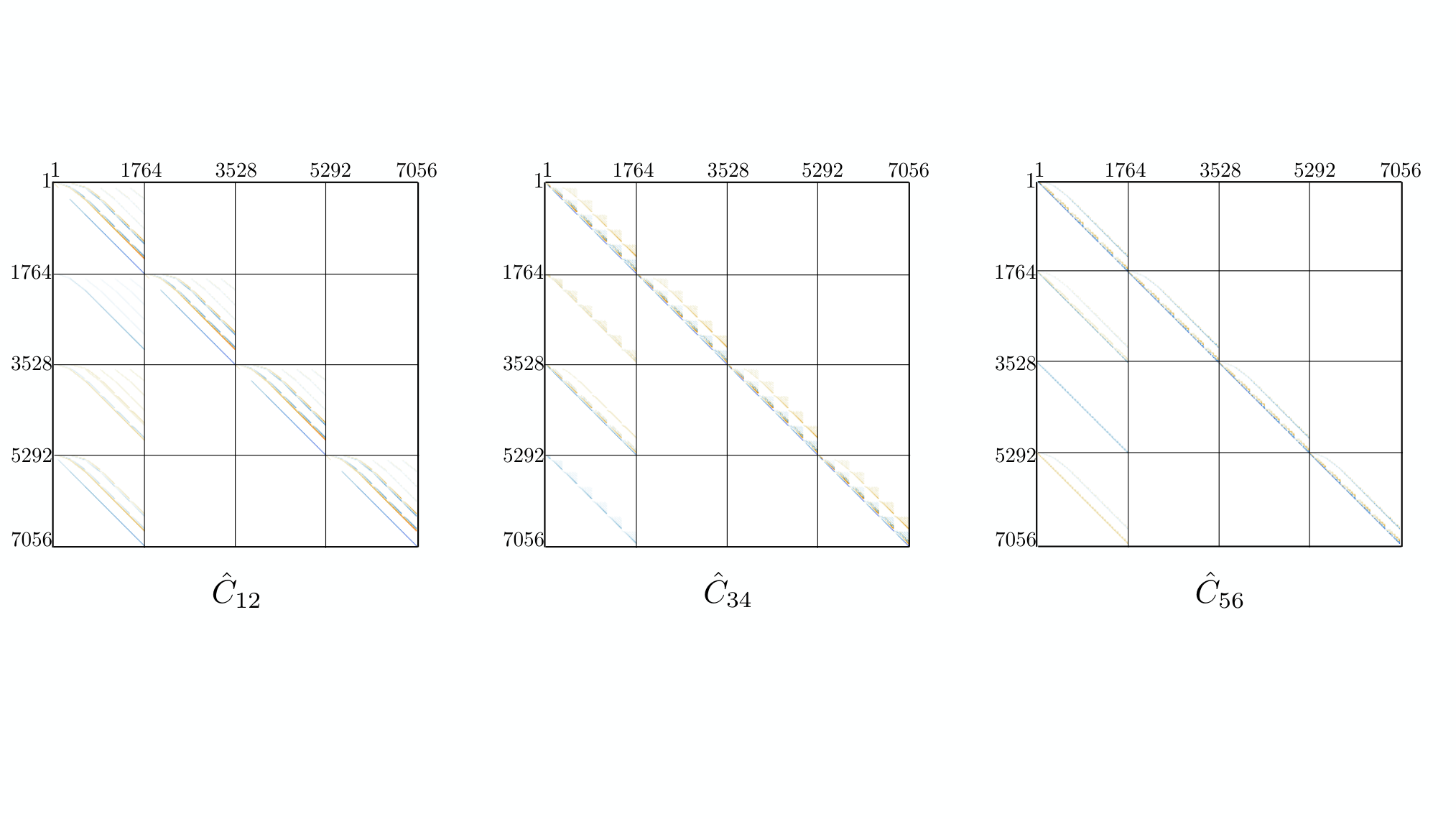
Refer to caption
Figure 6: The six point function in the snowflake OPE limit (ziz_{i}, z^i\hat{z}_{i} →0\rightarrow 0) can be expressed as a sum of monomials ∏iziai​z^ili\prod_{i}z_{i}^{a_{i}}\hat{z}_{i}^{l_{i}} which in perturbation theory can be dressed by log⁡(ui)\log(u_{i}). The action of the Casimir operators in this base of dressed monomials can be represented as sparse matrices which are plotted here for ai≤6a_{i}\leq 6, li≤2l_{i}\leq 2. The basis is restricted to l1+l2≤a3l_{1}+l_{2}\leq a_{3} and similar for the other aia_{i} as discused in the main text. At one loop, the basis can be divided into terms with no log\logs, or a single log⁡(u1)\log(u_{1}), log⁡(u2)\log(u_{2}) or log⁡(u3)\log(u_{3}), leading to the 4×44\times 4 block structure. The Casimir can remove l​o​glogs but never generate them, justifying the absence of off diagonal terms in the last three columns.

This way of extracting is very convenient. The data itself is organized in a simple manner, for given power of ziaiz_{i}^{a_{i}} the z^ili\hat{z}_{i}^{l_{i}} powers are such that l1+l2≤J3l_{1}+l_{2}\leq J_{3} is satisfied and analogously for the others lil_{i} and at one loop these powers can be dressed by ln⁡ui\ln u_{i}. An efficient way to do this extraction is transform the Casimir into a matrix that acts on a vector space created powers of zi,z^iz_{i},\hat{z}_{i} and ln⁡ui\ln u_{i} which then makes (51) into a matrix multiplication problem, see figure 6. Obviously we need to consider finite dimensional vector spaces so we take a cut off (Λi,Λ^i\Lambda_{i},\hat{\Lambda}_{i}) in the powers of zi,z^iz_{i},\hat{z}_{i}. This allows to extract OPE coefficients up to spin Ji=Λi,ℓi=Λ^iJ_{i}=\Lambda_{i},\ell_{i}=\hat{\Lambda}_{i}. With this we manage to extract around three hundred thousand OPE coefficients at one loop order which we will analyze in the next section.

E.1 Data

Perturbative results for three point functions with more than one spinning operator are considerably more complicated to compute than with just one operator with spin. While three point functions with one spinning operator have been computed, in 𝒩=4\mathcal{N}=4 SYM, up to three loops [21], three point functions with two spinning operators have only been computed up to one loop 1414 14 There are some results for low spinning operators up to two loops [19]. . In the following we will compute these three point functions at one loop for both one, two and three spinning operators by doing conformal block decomposition decomposition of a one loop six point function.

The starting point is the six point function of 20′20^{\prime} operators

(52) 𝒪2(x)=yIyJTr(ϕI(x)ϕJ),y2=0,I=1,…6\displaystyle\mathcal{O}_{2}(x)=y^{I}y^{J}\textrm{Tr}(\phi^{I}(x)\phi^{J}),\,\ \ \ y^{2}=0,\,\,\ \ \ I=1,\dots 6

which has been computed at one loop in [6] and it is expressed as a simple linear combination of one loop four point integrals Ii1​i2​i3​i4I_{i_{1}i_{2}i_{3}i_{4}}(see eq. (32,60-61) of [6] for the precise definition of the six point function)

(53) Ii1​i2​i3​i4=∫d4​x0xi1​02​xi2​02​xi3​02​xi4​02\displaystyle I_{i_{1}i_{2}i_{3}i_{4}}=\int\frac{d^{4}x_{0}}{x_{i_{1}0}^{2}x_{i_{2}0}^{2}x_{i_{3}0}^{2}x_{i_{4}0}^{2}}

which can be easily computed in terms of cross ratios.

We are interested in obtaining three point functions in the [0,2,0][0,2,0] representation of S​O​(6)SO(6) in the OPE. This can be achieved by projecting appropriately the null polarization vectors yy into this particular representation (see appendix B of [22] for details). Then we take the light-cone limits x122,x342,x562→0x_{12}^{2},x_{34}^{2},x_{56}^{2}\rightarrow 0 to focus on leading twist operators. At the end of this procedure we arrive at the following (tree level plus one loop) expression

(54) data =(x122​x342​x562)2​⟨𝒪2​(x1)​…​𝒪2​(x6)⟩|projection on [0,2,0]x122,x342,x562→0.\displaystyle=(x_{12}^{2}x_{34}^{2}x_{56}^{2})^{2}\langle\mathcal{O}_{2}(x_{1})\dots\mathcal{O}_{2}(x_{6})\rangle\bigg|_{\texttt{projection on $[0,2,0]$}\atop{x_{12}^{2},x_{34}^{2},x_{56}^{2}\rightarrow 0}}.
=∏i=13u2​i−1u2​i​Ui[3​u2​u4​U1​U2​(1+u6)+U1​U2​U3​(1+u2​u4​u6)24+\displaystyle=\prod_{i=1}^{3}\frac{{\color[rgb]{0,0.6,0}u_{2i-1}}}{u_{2i}U_{i}}\bigg[\frac{3u_{2}u_{4}{\color[rgb]{0,0,1}U_{1}}{\color[rgb]{0,0,1}U_{2}}(1+u_{6})+{\color[rgb]{0,0,1}U_{1}}{\color[rgb]{0,0,1}U_{2}}{\color[rgb]{0,0,1}U_{3}}(1+u_{2}u_{4}u_{6})}{24}+
−λ4(lnu1[U3lnu2(u4u6(U1−u2U2)+U2(U1−u2u6))\displaystyle-\frac{{\color[rgb]{1,0,0}\lambda}}{4}\bigg(\ln{\color[rgb]{0,0.6,0}u_{1}}\big[{\color[rgb]{0,0,1}U_{3}}\ln u_{2}(u_{4}u_{6}({\color[rgb]{0,0,1}U_{1}}-u_{2}{\color[rgb]{0,0,1}U_{2}})+{\color[rgb]{0,0,1}U_{2}}({\color[rgb]{0,0,1}U_{1}}-u_{2}u_{6}))
+U2​ln⁡u6​(u2​(u4​(1−u6)​U1−u6​U3)+U1​U3)+u4​u6​U3​ln⁡U2​((1+u2)​U1−u2​(1+U1)​U2)\displaystyle+{\color[rgb]{0,0,1}U_{2}}\ln u_{6}(u_{2}(u_{4}(1-u_{6}){\color[rgb]{0,0,1}U_{1}}-u_{6}{\color[rgb]{0,0,1}U_{3}})+{\color[rgb]{0,0,1}U_{1}}{\color[rgb]{0,0,1}U_{3}})+u_{4}u_{6}{\color[rgb]{0,0,1}U_{3}}\ln{\color[rgb]{0,0,1}U_{2}}((1+u_{2}){\color[rgb]{0,0,1}U_{1}}-u_{2}(1+{\color[rgb]{0,0,1}U_{1}}){\color[rgb]{0,0,1}U_{2}})
+U3lnU1(U2(u2u6−U1)+u4u6(u2U2−U1))]+lnu2[u2u6U3lnU3(U2−u4U1)\displaystyle+{\color[rgb]{0,0,1}U_{3}}\ln{\color[rgb]{0,0,1}U_{1}}({\color[rgb]{0,0,1}U_{2}}(u_{2}u_{6}-{\color[rgb]{0,0,1}U_{1}})+u_{4}u_{6}(u_{2}{\color[rgb]{0,0,1}U_{2}}-{\color[rgb]{0,0,1}U_{1}}))\big]+\ln u_{2}\big[u_{2}u_{6}{\color[rgb]{0,0,1}U_{3}}\ln{\color[rgb]{0,0,1}U_{3}}({\color[rgb]{0,0,1}U_{2}}-u_{4}{\color[rgb]{0,0,1}U_{1}})
+U1lnU2(u2u4(U2+u6U3)−U3(U2+u4u6))]+U2lnU1lnU2(U1U3+u2u6(u4U1−(1+u4)U3))\displaystyle+{\color[rgb]{0,0,1}U_{1}}\ln{\color[rgb]{0,0,1}U_{2}}(u_{2}u_{4}({\color[rgb]{0,0,1}U_{2}}+u_{6}{\color[rgb]{0,0,1}U_{3}})-{\color[rgb]{0,0,1}U_{3}}({\color[rgb]{0,0,1}U_{2}}+u_{4}u_{6}))\big]+{\color[rgb]{0,0,1}U_{2}}\ln{\color[rgb]{0,0,1}U_{1}}\ln{\color[rgb]{0,0,1}U_{2}}({\color[rgb]{0,0,1}U_{1}}{\color[rgb]{0,0,1}U_{3}}+u_{2}u_{6}(u_{4}{\color[rgb]{0,0,1}U_{1}}-(1+u_{4}){\color[rgb]{0,0,1}U_{3}}))
+u6​(u4​U1​U3+u2​(U2​U3−u4​U1​(U2+U3)))​Li2​(1−u2)\displaystyle+u_{6}(u_{4}{\color[rgb]{0,0,1}U_{1}}{\color[rgb]{0,0,1}U_{3}}+u_{2}({\color[rgb]{0,0,1}U_{2}}{\color[rgb]{0,0,1}U_{3}}-u_{4}{\color[rgb]{0,0,1}U_{1}}({\color[rgb]{0,0,1}U_{2}}+{\color[rgb]{0,0,1}U_{3}})))\texttt{Li}_{2}(1-u_{2})
+U2​(U1​U3−u2​u4​(U1+u6​U3​(U1−1)))​Li2​(1−U1)\displaystyle+{\color[rgb]{0,0,1}U_{2}}({\color[rgb]{0,0,1}U_{1}}{\color[rgb]{0,0,1}U_{3}}-u_{2}u_{4}({\color[rgb]{0,0,1}U_{1}}+u_{6}{\color[rgb]{0,0,1}U_{3}}({\color[rgb]{0,0,1}U_{1}}-1)))\texttt{Li}_{2}(1-{\color[rgb]{0,0,1}U_{1}})
+(U1​U3​(u4​u6+U2)+u2​(u4​U1​U2​(u6−1)+u6​U3​(U2​(u4​(U1−1)−1)−U1​u4)))​Li2​(1−u2U1)\displaystyle+\big({\color[rgb]{0,0,1}U_{1}}{\color[rgb]{0,0,1}U_{3}}(u_{4}u_{6}+{\color[rgb]{0,0,1}U_{2}})+u_{2}(u_{4}{\color[rgb]{0,0,1}U_{1}}{\color[rgb]{0,0,1}U_{2}}(u_{6}-1)+u_{6}{\color[rgb]{0,0,1}U_{3}}({\color[rgb]{0,0,1}U_{2}}(u_{4}({\color[rgb]{0,0,1}U_{1}}-1)-1)-{\color[rgb]{0,0,1}U_{1}}u_{4}))\big)\texttt{Li}_{2}\left(1-\frac{u_{2}}{{\color[rgb]{0,0,1}U_{1}}}\right)
+U2​(U1​U3−u2​u4​(U1+u6​U3​(U1−1)))​Li2​(1−u2​u4U3)\displaystyle+{\color[rgb]{0,0,1}U_{2}}({\color[rgb]{0,0,1}U_{1}}{\color[rgb]{0,0,1}U_{3}}-u_{2}u_{4}({\color[rgb]{0,0,1}U_{1}}+u_{6}{\color[rgb]{0,0,1}U_{3}}({\color[rgb]{0,0,1}U_{1}}-1)))\texttt{Li}_{2}\left(1-\frac{u_{2}u_{4}}{{\color[rgb]{0,0,1}U_{3}}}\right)
+u4(u6U1U3−u2U2(u6U3+U1(u6−1)))Li2(1−u2​U2U1))+two permutations]\displaystyle+u_{4}(u_{6}{\color[rgb]{0,0,1}U_{1}}{\color[rgb]{0,0,1}U_{3}}-u_{2}{\color[rgb]{0,0,1}U_{2}}(u_{6}{\color[rgb]{0,0,1}U_{3}}+{\color[rgb]{0,0,1}U_{1}}(u_{6}-1)))\texttt{Li}_{2}\left(1-\frac{u_{2}{\color[rgb]{0,0,1}U_{2}}}{{\color[rgb]{0,0,1}U_{1}}}\right)\bigg)+\texttt{two permutations}\bigg]
=∏i=13u2​i−1[1+∑i(zi+zi2)2+z1​z2+z1​z3+z2​z34−z2​z3​z^1+z1​z3​z^2+z1​z2​z^34+\displaystyle=\prod_{i=1}^{3}{\color[rgb]{0,0.6,0}u_{2i-1}}\bigg[1+\frac{\sum_{i}(z_{i}+z_{i}^{2})}{2}+\frac{z_{1}z_{2}+z_{1}z_{3}+z_{2}z_{3}}{4}-\frac{z_{2}z_{3}\hat{z}_{1}+z_{1}z_{3}\hat{z}_{2}+z_{1}z_{2}\hat{z}_{3}}{4}+
(55) +λ(z12(lnu1−2)+z22(lnu3−2)+z32(lnu5−2))+…]\displaystyle+{\color[rgb]{1,0,0}\lambda}\big(z_{1}^{2}(\ln{\color[rgb]{0,0.6,0}u_{1}}-2)+z_{2}^{2}(\ln{\color[rgb]{0,0.6,0}u_{3}}-2)+z_{3}^{2}(\ln{\color[rgb]{0,0.6,0}u_{5}}-2)\big)+\dots\bigg]

where the two permutations are just given by ui,Ui→ui+2,Ui+2;ui+4,Ui+4u_{i},U_{i}\rightarrow u_{i+2},U_{i+2};u_{i+4},U_{i+4} and where the dots in the last line stand for higher order powers in ziz_{i}. This is precisely the object that enters in (51) and that can be used to extract OPE coefficients of three spinning operators at one loop. The last line is transformed into a vector of the monomials and log\logs which is then acted by the Casimir matrix of figure 6 to efficiently extract all the needed OPE data.

Through this method we extracted over three hundred thousand OPE coefficients. Both the notebook used for extraction as well as a sample of the result are presented in the attached Mathematica notebooks. Our goal now is to write such data as an expression analytically both in spins and polarizations. In the next three sections we display the structure constant for one, two and three spinning operators.

Appendix F One Loop Explorations

F.1 One spinning operator

The structure constants for one spinning operator have been studied extensively in the literature. The first non trivial computation of these three point functions in 𝒩=4\mathcal{N}=4 was done at one loop level in [23] via conformal block decomposition of a four point function. It is the most efficient way of computing these three point function. Using this method the structure constants with one spinning operator have been computed up to three loops for any spin in [21] and is known up to five loops for spin two [24].

The one loop structure constant simply reads

(56) C^1-loop∘∘∙=4S1(J)2−4S1(J)S1(2J)−2S2(J)\hat{C}^{\circ\circ\bullet}_{\texttt{1-loop}}=4S_{1}(J)^{2}-4S_{1}(J)S_{1}(2J)-2S_{2}(J)

where SiS_{i} are the harmonic functions.

To set the coupling convention let us quote here the dimension of these operators

(57) ΔJ=2+J+8​λ​S1​(J)+O⁡(λ2)\Delta_{J}=2+J+8\lambda S_{1}(J)+O(\lambda^{2})

so that from large spin we read

(58) f=8​λ+O⁡(λ2),andg=8​λ​γE+O⁡(λ2).f=8\lambda+O(\lambda^{2})\,,\quad\text{and}\quad g=8\lambda\gamma_{E}+O(\lambda^{2})\,.

F.2 Two spinning operators

Here we complete Bianchi’s computation [19] for the one loop structure constant

C^∘∙∙1-loop\displaystyle\hat{C}^{\circ\bullet\bullet}_{\texttt{1-loop}} =4​(S1​(J1)+S1​(J2))​∑i=1ℓ(J1+J2+1i)​(ℓi)i​(J1i)​(J2i)−4​(J1+1)​(J2+1)J1+J2+2​∑i=1ℓ(J1+J2+2i)​aiℓi​(J1i)​(J2i)+\displaystyle=4\left(S_{1}(J_{1})+S_{1}(J_{2})\right)\sum_{i=1}^{\ell}\frac{\binom{J_{1}+J_{2}+1}{i}\binom{\ell}{i}}{i\binom{J_{1}}{i}\binom{J_{2}}{i}}-4\frac{(J_{1}+1)(J_{2}+1)}{J_{1}+J_{2}+2}\sum_{i=1}^{\ell}\frac{\binom{J_{1}+J_{2}+2}{i}a_{i}^{\ell}}{i\binom{J_{1}}{i}\binom{J_{2}}{i}}+
(59) +∑i=124S1(Ji)2−4S1(Ji)S1(2Ji)−2S2(Ji)\displaystyle+\sum_{i=1}^{2}4S_{1}(J_{i})^{2}-4S_{1}(J_{i})S_{1}(2J_{i})-2S_{2}(J_{i})

where the constants aiℓa_{i}^{\ell} were only known in special limiting cases. They are given by

(60) aiℓ=(−1)i2​(−S1​(ℓ)2−S2​(ℓ)+2​∑k=2i(−1)k​(lk−1)k−1​(S1​(k−2)+S1​(ℓ))).a_{i}^{\ell}=\frac{(-1)^{i}}{2}\left(-S_{1}(\ell)^{2}-S_{2}(\ell)+2\sum_{k=2}^{i}\frac{(-1)^{k}\binom{l}{k-1}}{k-1}\left(S_{1}(k-2)+S_{1}(\ell)\right)\right)\,.

For i=1i=1 and for i=ℓi=\ell it simplifies to the two previously known special cases (4.5) and (4.6) in [19]. This one loop structure constant can also be rewritten as (62), where

(61) 𝔹⁡(j,l)=(−1)l​(jl).\mathbb{B}(j,l)=(-1)^{l}\binom{j}{l}\,.

Having the full expression for the structure constant at one loop in the form of (62) allow us to study the physics of this correlator at large spin and polarizations, with ℓJi\frac{\ell}{J_{i}} fixed. As discussed in section 5, this serves as a toy model for the large spin limit of three point functions of spinning operators and its relation to the null hexagonal Wilson loops.

C^∘∙∙1-loop\displaystyle\hat{C}^{\circ\bullet\bullet}_{\texttt{1-loop}} =8​S1​(J1)2−4​S1​(J1)​S1​(2​J1)+8​S1​(J1)​S1​(J2)+8​S1​(J2)2−4​S1​(J2)​S1​(2​J2)+\displaystyle=8S_{1}(J_{1})^{2}-4S_{1}(J_{1})S_{1}(2J_{1})+8S_{1}(J_{1})S_{1}(J_{2})+8S_{1}(J_{2})^{2}-4S_{1}(J_{2})S_{1}(2J_{2})+
−4​S1​(J1)​S1​(J1−ℓ)−4​S1​(J2)​S1​(J1−ℓ)−4​S1​(J1)​S1​(J2−ℓ)−4​S1​(J2)​S1​(J2−ℓ)+\displaystyle-4S_{1}(J_{1})S_{1}(J_{1}-\ell)-4S_{1}(J_{2})S_{1}(J_{1}-\ell)-4S_{1}(J_{1})S_{1}(J_{2}-\ell)-4S_{1}(J_{2})S_{1}(J_{2}-\ell)+
−4​S1​(J1)​S1​(ℓ)−4​S1​(J2)​S1​(ℓ)+4​S1​(J1−ℓ)​S1​(ℓ)+4​S1​(J2−ℓ)​S1​(ℓ)−2​S1​(ℓ)2+\displaystyle-4S_{1}(J_{1})S_{1}(\ell)-4S_{1}(J_{2})S_{1}(\ell)+4S_{1}(J_{1}-\ell)S_{1}(\ell)+4S_{1}(J_{2}-\ell)S_{1}(\ell)-2S_{1}(\ell)^{2}+
−2​S2​(J1)−2​S2​(J2)−2​S2​(ℓ)−4​∑p=1∞((𝔹⁡(J1,ℓ−p)𝔹⁡(J1,ℓ)+𝔹⁡(J2,ℓ−p)𝔹⁡(J2,ℓ))​S1​(p−1)p+CLOSE\displaystyle-2S_{2}(J_{1})-2S_{2}(J_{2})-2S_{2}(\ell)-4\sum_{p=1}^{\infty}\Bigg(\left(\frac{\mathbb{B}(J_{1},\ell-p)}{\mathbb{B}(J_{1},\ell)}+\frac{\mathbb{B}(J_{2},\ell-p)}{\mathbb{B}(J_{2},\ell)}\right)\frac{S_{1}(p-1)}{p}+
+4(S1(J1)+S1(J2)−S1(ℓ))𝔹⁡(J1,ℓ−p)𝔹⁡(J1,ℓ)𝔹⁡(J2,ℓ−p)𝔹⁡(J2,ℓ)1p−4𝔹⁡(J1,ℓ−p)𝔹⁡(J1,ℓ)×\displaystyle+4(S_{1}(J_{1})+S_{1}(J_{2})-S_{1}(\ell))\frac{\mathbb{B}(J_{1},\ell-p)}{\mathbb{B}(J_{1},\ell)}\frac{\mathbb{B}(J_{2},\ell-p)}{\mathbb{B}(J_{2},\ell)}\frac{1}{p}-4\frac{\mathbb{B}(J_{1},\ell-p)}{\mathbb{B}(J_{1},\ell)}\times
×𝔹⁡(J2,ℓ−p)𝔹⁡(J2,ℓ)​S1​(p)+S1​(ℓ−p)−S1​(ℓ)p+∑q=1p−1𝔹⁡(J1,ℓ−p)𝔹⁡(J1,ℓ)​𝔹⁡(J2,ℓ−q)𝔹⁡(J2,ℓ)​1(p−q)​p\displaystyle\times\frac{\mathbb{B}(J_{2},\ell-p)}{\mathbb{B}(J_{2},\ell)}\frac{S_{1}(p)+S_{1}(\ell-p)-S_{1}(\ell)}{p}+\sum_{q=1}^{p-1}\frac{\mathbb{B}(J_{1},\ell-p)}{\mathbb{B}(J_{1},\ell)}\frac{\mathbb{B}(J_{2},\ell-q)}{\mathbb{B}(J_{2},\ell)}\frac{1}{(p-q)p}
(62) +∑q=p+1∞𝔹⁡(J1,ℓ−p)𝔹⁡(J1,ℓ)𝔹⁡(J2,ℓ−q)𝔹⁡(J2,ℓ)1(q−p)​q).\displaystyle+\sum_{q=p+1}^{\infty}\frac{\mathbb{B}(J_{1},\ell-p)}{\mathbb{B}(J_{1},\ell)}\frac{\mathbb{B}(J_{2},\ell-q)}{\mathbb{B}(J_{2},\ell)}\frac{1}{(q-p)q}\Bigg).

There are two regimes of interest, depending on whether ℓ\ell is before or after ℓ∗≡J1​J2(J1+J2)\ell_{*}\equiv\frac{J_{1}J_{2}}{\left(J_{1}+J_{2}\right)}.1515 15 Note that the tree level three point function, given by Ctree∙∙∘=Γ⁡(J1+1)​Γ​(J2+1)Γ⁡(2​J1+1)​Γ​(2​J2+1)​Γ​(J1−ℓ+1)​Γ​(J2−ℓ+1)​Γ​(ℓ+1),C_{\text{tree}}^{\bullet\bullet\circ}=\frac{\Gamma(J_{1}+1)\Gamma(J_{2}+1)}{\sqrt{\Gamma(2J_{1}+1)\Gamma(2J_{2}+1)}\Gamma(J_{1}-\ell+1)\Gamma(J_{2}-\ell+1)\Gamma(\ell+1)}, approaches a gaussian centered at ℓ∗\ell_{*} in the large spin limit. Before ℓ∗\ell_{*} we obtain the order one result

(63) C^∙∙∘1-loop→J1,J2,ℓ→∞\displaystyle\hat{C}^{\bullet\bullet\circ}_{\texttt{1-loop}}\xrightarrow{J_{1},J_{2},\ell\rightarrow\infty} −π2−4​log⁡(2)​log⁡(J1​J2​e2​γE)−2​log2⁡(ℓ​eγE)\displaystyle-\pi^{2}-4\log(2)\log\left(J_{1}J_{2}e^{2\gamma_{E}}\right)-2\log^{2}\left(\ell e^{\gamma_{E}}\right)
−2​log⁡(1−ℓJ1−ℓJ2)​log⁡(e2​γE​J12​J22ℓ2​(1−ℓJ1−ℓJ2))\displaystyle-2\log\Big(1-\frac{\ell}{J_{1}}-\frac{\ell}{J_{2}}\Big)\log\Big(\frac{e^{2\gamma_{E}}J_{1}^{2}J_{2}^{2}}{\ell^{2}}\big(1-\frac{\ell}{J_{1}}-\frac{\ell}{J_{2}}\big)\Big)

while after ℓ∗\ell_{*} we obtain the exponentially large expression

C^∙∙∘1-loop→J1,J2,ℓ→∞\displaystyle\hat{C}^{\bullet\bullet\circ}_{\texttt{1-loop}}\xrightarrow{J_{1},J_{2},\ell\rightarrow\infty} J1−2​J1−1J2−2​J2−1(J1+J2)J1+J2+32ℓ2​ℓ+1(J1−ℓ)J1−ℓ+12(J2−ℓ)J2−ℓ+12J1​J2−J1​ℓ−J2​ℓ×\displaystyle\frac{J_{1}^{-2J_{1}-1}J_{2}^{-2J_{2}-1}\left(J_{1}+J_{2}\right){}^{J_{1}+J_{2}+\frac{3}{2}}\ell^{2\ell+1}\left(J_{1}-\ell\right){}^{J_{1}-\ell+\frac{1}{2}}\left(J_{2}-\ell\right){}^{J_{2}-\ell+\frac{1}{2}}}{J_{1}J_{2}-J_{1}\ell-J_{2}\ell}\times
(64) ×4​2​π​log⁡(ℓJ1+ℓJ2−1).\displaystyle\times 4\sqrt{2\pi}\log\left(\frac{\ell}{J_{1}}+\frac{\ell}{J_{2}}-1\right).

Note that the singular point ℓ∗\ell_{*} is reminiscent of the singularities encountered in the U⁡(ℓ)U(\ell) map, equation (12). The log\log singularities at ℓ∗\ell_{*} in (63) should therefore be compared with the log\log singularities of the hexagonal Wilson loop at Ui=0U_{i}=0, see (26). This justifies treating C∙∙∘C^{\bullet\bullet\circ} as a toy model for the transition in behaviour of C∙∙∙C^{\bullet\bullet\bullet} from the space-like region to the time-like region in section 5.

Lets comment on how these results can be derived. The only non-trivial pieces in (62) are the sums, of which there are two types, that with a single ratio of binomials, as in the third line, and those with a product of ratio of binomials, as in the last three lines. First we analyze the latter.

Binomials (jl)\binom{j}{l}, in the large jj limit with ℓj\frac{\ell}{j} fixed approach gaussians with mean j/2j/2 and standard deviation j/2\sqrt{j}/2. The product of binomials in the denominators therefore approach gaussians1616 16 The product of gaussians is a gaussian. with mean ℓ∗=J1​J2J1+J2\ell_{*}=\frac{J_{1}J_{2}}{J_{1}+J_{2}} and standard deviation O⁡(J)O(\sqrt{J}). Similar happens in the numerators only that arguments are shifted. The sum indices pp and qq being positive, we see that if ℓ<ℓ∗\ell<\ell_{*} so that the denominator is evaluated to the left of the maximum, large pp and qq are exponentially suppressed relative to pp, qq of order one. In this limit, the sums are easily evaluated. For example, in the fifth line we have the simplification

(65) ∑p=1l(𝔹⁡(J1,ℓ−p)𝔹⁡(J1,ℓ)​𝔹⁡(J2,ℓ−p)𝔹⁡(J2,ℓ)​1p→(ℓ2(J1−ℓ)​(J2−l))p​1p)=−log⁡(ℓ⁡(J1+J2)−J1​J2(J1−ℓ)​(J2−ℓ)).\sum_{p=1}^{l}\left(\frac{\mathbb{B}(J_{1},\ell-p)}{\mathbb{B}(J_{1},\ell)}\frac{\mathbb{B}(J_{2},\ell-p)}{\mathbb{B}(J_{2},\ell)}\frac{1}{p}\rightarrow\left(\frac{\ell^{2}}{(J_{1}-\ell)(J_{2}-l)}\right)^{p}\frac{1}{p}\right)=-\log\left(\frac{\ell(J_{1}+J_{2})-J_{1}J_{2}}{(J_{1}-\ell)(J_{2}-\ell)}\right).

On the other hand, if ℓ>ℓ∗\ell>\ell_{*}, provided pp and qq are O⁡(J)O(J), we can tune the indices so that the numerator sits at the top of the gaussian. The sums are therefore evaluated by saddle point and we obtain the exponential expression in (F.2).

For the summand with a single ratio of binomials, for similar reasons, pp of order one dominates when ℓ<ℓ∗\ell<\ell_{*} and log\logs are generated. However, for this term there are no exponential contributions when ℓ>ℓ∗\ell>\ell_{*} due to the oscillating phase in (61). Therefore this term can be neglected in the ℓ>ℓ∗\ell>\ell_{*} regime.

Finally, we note a sum rule for the one-loop sum of structure constants, valid at finite J1J_{1} and J2J_{2}:

(66) ∑ℓC1-loop∙∙∘=4(S1(J1)+S1(J2))S1(J1+J2)−∑i=124S1(Ji)S1(2Ji)+2S2(Ji),\sum_{\ell}C^{\bullet\bullet\circ}_{\texttt{1-loop}}=4\left(S_{1}(J_{1})+S_{1}(J_{2})\right)S_{1}(J_{1}+J_{2})-\sum_{i=1}^{2}4S_{1}(J_{i})S_{1}(2J_{i})+2S_{2}(J_{i})\,,

note that this sums is for the full one loop correction to the structure constants (C=Ctree+C1-loopC=C_{\texttt{tree}}+C_{\texttt{1-loop}}) and not the correction normalized by tree level (C^\hat{C}).

F.3 Three spinning operators

For three spinning operators we were not able to find an expression analogous (59) or (62), which is analytical both in spin and polarizations. In this section we present a general expression for the one-loop structure constant in terms of unknown coefficients that we could not fix entirely. However, when considering small polarizations (where we have abundant perturbative data) we were able to fix such coefficients and arrive in an analytic expression for the structure constant in terms of the spins JiJ_{i}, such as (72).

We start by parametrizing the one-loop structure constant as the sum of three terms

(67) C^ℓ1,ℓ2,ℓ3J1,J2,J3=𝒳J1,J2,J3+𝒴ℓ1,ℓ2,ℓ3J1,J2,J3+𝒵ℓ1,ℓ2,ℓ3J1,J2,J3\hat{C}^{J_{1},J_{2},J_{3}}_{\ell_{1},\ell_{2},\ell_{3}}=\mathcal{X}^{J_{1},J_{2},J_{3}}+\mathcal{Y}^{J_{1},J_{2},J_{3}}_{\ell_{1},\ell_{2},\ell_{3}}+\mathcal{Z}^{J_{1},J_{2},J_{3}}_{\ell_{1},\ell_{2},\ell_{3}}

The first term of (67) is a generalization of the one spin structure constant (56), and it is simply given by

𝒳J1,J2,J3\displaystyle\mathcal{X}^{J_{1},J_{2},J_{3}} =4​S1​(J1)2−4​S1​(J1)​S1​(2​J1)−2​S2​(J1)+4​S1​(J2)2−4​S1​(J2)​S1​(2​J2)+\displaystyle=4S_{1}(J_{1})^{2}-4S_{1}(J_{1})S_{1}(2J_{1})-2S_{2}(J_{1})+4S_{1}(J_{2})^{2}-4S_{1}(J_{2})S_{1}(2J_{2})+
(68) −2​S2​(J2)+4​S1​(J3)2−4​S1​(J3)​S1​(2​J3)−2​S2​(J3)\displaystyle-2S_{2}(J_{2})+4S_{1}(J_{3})^{2}-4S_{1}(J_{3})S_{1}(2J_{3})-2S_{2}(J_{3})

this term gives the one-loop structure constants for vanishing polarizations (ℓi=0\ell_{i}=0).

The second term of (67) is inspired in the two spin structure constants (59), which reads

𝒴ℓ1,ℓ2,ℓ3J1,J2,J3\displaystyle\mathcal{Y}^{J_{1},J_{2},J_{3}}_{\ell_{1},\ell_{2},\ell_{3}} =4​(S1​(J1)+S1​(J2))​∑i=1ℓ3((J1+J2+1i)​(ℓ3i)i​(J1i)​(J2i))−4​(J1+1)​(J2+1)J1+J2+2​∑i=1ℓ3((J1+J2+2i)​aiℓ3i​(J1i)​(J2i))+\displaystyle=4\left(S_{1}(J_{1})+S_{1}(J_{2})\right)\sum_{i=1}^{\ell_{3}}\left(\frac{\binom{J_{1}+J_{2}+1}{i}\binom{\ell_{3}}{i}}{i\binom{J_{1}}{i}\binom{J_{2}}{i}}\right)-4\frac{(J_{1}+1)(J_{2}+1)}{J_{1}+J_{2}+2}\sum_{i=1}^{\ell_{3}}\left(\frac{\binom{J_{1}+J_{2}+2}{i}a_{i}^{\ell_{3}}}{i\binom{J_{1}}{i}\binom{J_{2}}{i}}\right)+
+4(S1(J1)+S1(J3))∑i=1ℓ2((J1+J3+1i)​(ℓ2i)i​(J1i)​(J3i))−4(J1+1)​(J3+1)J1+J3+2∑i=1ℓ2((J1+J3+2i)​aiℓ2i​(J1i)​(J3i))+\displaystyle+4\left(S_{1}(J_{1})+S_{1}(J_{3})\right)\sum_{i=1}^{\ell_{2}}\left(\frac{\binom{J_{1}+J_{3}+1}{i}\binom{\ell_{2}}{i}}{i\binom{J_{1}}{i}\binom{J_{3}}{i}}\right)-4\frac{(J_{1}+1)(J_{3}+1)}{J_{1}+J_{3}+2}\sum_{i=1}^{\ell_{2}}\left(\frac{\binom{J_{1}+J_{3}+2}{i}a_{i}^{\ell_{2}}}{i\binom{J_{1}}{i}\binom{J_{3}}{i}}\right)+
+4(S1(J2)+S1(J3))∑i=1ℓ1((J2+J3+1i)​(ℓ1i)i​(J2i)​(J3i))−4(J2+1)​(J3+1)J2+J3+2∑i=1ℓ1((J2+J3+2i)​aiℓ1i​(J2i)​(J3i))+\displaystyle+4\left(S_{1}(J_{2})+S_{1}(J_{3})\right)\sum_{i=1}^{\ell_{1}}\left(\frac{\binom{J_{2}+J_{3}+1}{i}\binom{\ell_{1}}{i}}{i\binom{J_{2}}{i}\binom{J_{3}}{i}}\right)-4\frac{(J_{2}+1)(J_{3}+1)}{J_{2}+J_{3}+2}\sum_{i=1}^{\ell_{1}}\left(\frac{\binom{J_{2}+J_{3}+2}{i}a_{i}^{\ell_{1}}}{i\binom{J_{2}}{i}\binom{J_{3}}{i}}\right)+
(69) +4∑i=13S1(ℓi)S1(ji).\displaystyle+4\sum_{i=1}^{3}S_{1}(\ell_{i})S_{1}(j_{i}).

This expression is a simple symmetrization of (59), except the last line, which does not exist in the context of two spinning operators. When combined with 𝒳J1,J2,J3\mathcal{X}^{J_{1},J_{2},J_{3}} it gives the structure constants with two vanishing polarizations (C^0,0,ℓJ1,J2,J3\hat{C}^{J_{1},J_{2},J_{3}}_{0,0,\ell}).

Through lengthy explorations of the extracted one loop data and inspired by [19] we were able to parametrize any one-loop structure constant via the following ansatz

(70) 𝒵ℓ1,ℓ2,ℓ3J1,J2,J3=q⁡(J1,J2,J3,ℓ1,ℓ2)+q⁡(J2,J3,J1,ℓ2,ℓ3)+q⁡(J3,J1,J2,ℓ3,ℓ1)\mathcal{Z}^{J_{1},J_{2},J_{3}}_{\ell_{1},\ell_{2},\ell_{3}}=q\left(J_{1},J_{2},J_{3},\ell_{1},\ell_{2}\right)+q\left(J_{2},J_{3},J_{1},\ell_{2},\ell_{3}\right)+q\left(J_{3},J_{1},J_{2},\ell_{3},\ell_{1}\right)

where

q⁡(j1,j2,j3,l1,l2)(1+j1)​(1+j2)\displaystyle\frac{q\left(j_{1},j_{2},j_{3},l_{1},l_{2}\right)}{(1+j_{1})(1+j_{2})} =(1+j3)​∑n=1l2∑m=1l1∑p=1l1+l2βl1,l2n,m,p​𝔹⁡(j1,l2−n)𝔹⁡(j1,l2)​𝔹⁡(j2,l1−m)𝔹⁡(j2,l1)​𝔹⁡(j3,l1+l2−p)𝔹⁡(j3,l1+l2)+\displaystyle=(1+j_{3})\sum_{n=1}^{l_{2}}\sum_{m=1}^{l_{1}}\sum_{p=1}^{l_{1}+l_{2}}\beta^{n,m,p}_{l_{1},l_{2}}\frac{\mathbb{B}(j_{1},l_{2}-n)}{\mathbb{B}(j_{1},l_{2})}\frac{\mathbb{B}(j_{2},l_{1}-m)}{\mathbb{B}(j_{2},l_{1})}\frac{\mathbb{B}(j_{3},l_{1}+l_{2}-p)}{\mathbb{B}(j_{3},l_{1}+l_{2})}+
(71) ∑n=1l2∑m=1l1∑p=n+ml1+l2γl1,l2n,m,p​𝔹⁡(j1,l2−n)𝔹⁡(j1,l2)​𝔹⁡(j2,l1−m)𝔹⁡(j2,l1)​𝔹⁡(j3,l1+l2−p)𝔹⁡(j3,l1+l2)​S1​(j3)\displaystyle\sum_{n=1}^{l_{2}}\sum_{m=1}^{l_{1}}\sum_{p=n+m}^{l_{1}+l_{2}}\gamma^{n,m,p}_{l_{1},l_{2}}\frac{\mathbb{B}(j_{1},l_{2}-n)}{\mathbb{B}(j_{1},l_{2})}\frac{\mathbb{B}(j_{2},l_{1}-m)}{\mathbb{B}(j_{2},l_{1})}\frac{\mathbb{B}(j_{3},l_{1}+l_{2}-p)}{\mathbb{B}(j_{3},l_{1}+l_{2})}S_{1}(j_{3})

with 𝔹\mathbb{B}, defined in (61) and being βli,ljn,m,p\beta^{n,m,p}_{l_{i},l_{j}} and γli,ljn,m,p\gamma^{n,m,p}_{l_{i},l_{j}} unknown coefficients. We were able to fix all γli,ljn,m,p\gamma^{n,m,p}_{l_{i},l_{j}} coefficients and a large portion of the βli,ljn,m,p\beta^{n,m,p}_{l_{i},l_{j}}, by comparing this ansatz with perturbative data and large spin expansions.

By matching with the extracted perturbative data we were able to fix all the γli,ljn,m,p\gamma^{n,m,p}_{l_{i},l_{j}} coefficients for polarizations up to ℓmax=5\ell_{\max}=5 and all the βl1,l2n,m,p\beta^{n,m,p}_{l_{1},l_{2}} for polarizations up to ℓmax=3\ell_{\max}=3, being expression (72) below an explicit example with polarizations {ℓ1=1,ℓ2=2,ℓ3=3}\{\ell_{1}=1,\ell_{2}=2,\ell_{3}=3\}.

C^1,2,3J1,J2,J3\displaystyle\hat{C}^{J_{1},J_{2},J_{3}}_{1,2,3} =𝒳J1,J2,J3+𝒴1,2,3J1,J2,J3+((1+J2)​(1+J3)​S1​(J1)𝔹⁡(J2,3)​𝔹​(J3,2)​𝔹​(J1,5))​(45−8​J215+13​J1​J230+CLOSE\displaystyle=\mathcal{X}^{J_{1},J_{2},J_{3}}+\mathcal{Y}^{J_{1},J_{2},J_{3}}_{1,2,3}+\Bigg(\frac{(1+J_{2})(1+J_{3})S_{1}(J_{1})}{\mathbb{B}(J_{2},3)\mathbb{B}(J_{3},2)\mathbb{B}(J_{1},5)}\Bigg)\Bigg(\frac{4}{5}-\frac{8J_{2}}{15}+\frac{13J_{1}J_{2}}{30}+
−J12​J230+2​J2215−2​J1​J2215+J12​J2230−2​J35+J1​J35+4​J2​J315−31​J1​J260+J12​J2​J35+\displaystyle-\frac{J_{1}^{2}J_{2}}{30}+\frac{2J_{2}^{2}}{15}-\frac{2J_{1}J_{2}^{2}}{15}+\frac{J_{1}^{2}J_{2}^{2}}{30}-\frac{2J_{3}}{5}+\frac{J_{1}J_{3}}{5}+\frac{4J_{2}J_{3}}{15}-\frac{31J_{1}J_{2}}{60}+\frac{J_{1}^{2}J_{2}J_{3}}{5}+
OPENJ13​J2​J360−J22​J315+J1​J22​J36−J12​J22​J310+J13​J22​J360)+\displaystyle\frac{J_{1}^{3}J_{2}J_{3}}{60}-\frac{J_{2}^{2}J_{3}}{15}+\frac{J_{1}J_{2}^{2}J_{3}}{6}-\frac{J_{1}^{2}J_{2}^{2}J_{3}}{10}+\frac{J_{1}^{3}J_{2}^{2}J_{3}}{60}\Bigg)+
+((1+J1)​(1+J3)​S1​(J2)𝔹⁡(J1,3)​𝔹​(J3,1)​𝔹​(J2,4))​(1−2​J13+J126+3​J1​J24−J12​J24−J1​J2212+J12​J2212)+\displaystyle+\Bigg(\frac{(1+J_{1})(1+J_{3})S_{1}(J_{2})}{\mathbb{B}(J_{1},3)\mathbb{B}(J_{3},1)\mathbb{B}(J_{2},4)}\Bigg)\Bigg(1-\frac{2J_{1}}{3}+\frac{J_{1}^{2}}{6}+\frac{3J_{1}J_{2}}{4}-\frac{J_{1}^{2}J_{2}}{4}-\frac{J_{1}J_{2}^{2}}{12}+\frac{J_{1}^{2}J_{2}^{2}}{12}\Bigg)+
+((1+J1)​(1+J2)​S1​(J3)𝔹⁡(J1,2)​𝔹​(J2,1)​𝔹​(J3,3))​(43−2​J13+2​J1​J33)+\displaystyle+\Bigg(\frac{(1+J_{1})(1+J_{2})S_{1}(J_{3})}{\mathbb{B}(J_{1},2)\mathbb{B}(J_{2},1)\mathbb{B}(J_{3},3)}\Bigg)\Bigg(\frac{4}{3}-\frac{2J_{1}}{3}+\frac{2J_{1}J_{3}}{3}\Bigg)+
+((1+J1)​(1+J2)​(1+J3)𝔹⁡(J1,5)​𝔹​(J2,4)​𝔹​(J3,3))​(−1760−29​J1720+71​J12864−61​J132160+13​J144320+CLOSE\displaystyle+\Bigg(\frac{(1+J_{1})(1+J_{2})(1+J_{3})}{\mathbb{B}(J_{1},5)\mathbb{B}(J_{2},4)\mathbb{B}(J_{3},3)}\Bigg)\Bigg(-\frac{17}{60}-\frac{29J_{1}}{720}+\frac{71J_{1}^{2}}{864}-\frac{61J_{1}^{3}}{2160}+\frac{13J_{1}^{4}}{4320}+
+13​J2120+623​J1​J24320−5269​J12​J225920+877​J13​J212960−187​J14​J225920−7​J22270−41​J1​J22405+859​J12​J226480+\displaystyle+\frac{13J_{2}}{120}+\frac{623J_{1}J_{2}}{4320}-\frac{5269J_{1}^{2}J_{2}}{25920}+\frac{877J_{1}^{3}J_{2}}{12960}-\frac{187J_{1}^{4}J_{2}}{25920}-\frac{7J_{2}^{2}}{270}-\frac{41J_{1}J_{2}^{2}}{405}+\frac{859J_{1}^{2}J_{2}^{2}}{6480}+
−1177​J13​J2225920+25​J14​J225184+J23270+119​J1​J236480−103​J12​J234320+227​J13​J2325920−5​J14​J235184+29​J3120+\displaystyle-\frac{1177J_{1}^{3}J_{2}^{2}}{25920}+\frac{25J_{1}^{4}J_{2}^{2}}{5184}+\frac{J_{2}^{3}}{270}+\frac{119J_{1}J_{2}^{3}}{6480}-\frac{103J_{1}^{2}J_{2}^{3}}{4320}+\frac{227J_{1}^{3}J_{2}^{3}}{25920}-\frac{5J_{1}^{4}J_{2}^{3}}{5184}+\frac{29J_{3}}{120}+
+167​J1​J31440−173​J12​J3960+83​J13​J31440−17​J14​J32880+37​J2​J3240−153​J1​J2​J3320+2393​J12​J2​J35760+\displaystyle+\frac{167J_{1}J_{3}}{1440}-\frac{173J_{1}^{2}J_{3}}{960}+\frac{83J_{1}^{3}J_{3}}{1440}-\frac{17J_{1}^{4}J_{3}}{2880}+\frac{37J_{2}J_{3}}{240}-\frac{153J_{1}J_{2}J_{3}}{320}+\frac{2393J_{1}^{2}J_{2}J_{3}}{5760}+
−569​J13​J2​J34320+239​J14​J2​J317280−73​J22​J3540+215​J1​J22​J3648−1399​J12​J22​J35184+1103​J13​J22​J312960+\displaystyle-\frac{569J_{1}^{3}J_{2}J_{3}}{4320}+\frac{239J_{1}^{4}J_{2}J_{3}}{17280}-\frac{73J_{2}^{2}J_{3}}{540}+\frac{215J_{1}J_{2}^{2}J_{3}}{648}-\frac{1399J_{1}^{2}J_{2}^{2}J_{3}}{5184}+\frac{1103J_{1}^{3}J_{2}^{2}J_{3}}{12960}+
−47​J14​J22​J35184+13​J23​J3540−49​J1​J23​J3810+1277​J12​J23​J325920−83​J13​J23​J35184+23​J14​J23​J312960−J3215+\displaystyle-\frac{47J_{1}^{4}J_{2}^{2}J_{3}}{5184}+\frac{13J_{2}^{3}J_{3}}{540}-\frac{49J_{1}J_{2}^{3}J_{3}}{810}+\frac{1277J_{1}^{2}J_{2}^{3}J_{3}}{25920}-\frac{83J_{1}^{3}J_{2}^{3}J_{3}}{5184}+\frac{23J_{1}^{4}J_{2}^{3}J_{3}}{12960}-\frac{J_{3}^{2}}{15}+
−11​J1​J32288+125​J12​J321728−209​J13​J328640+11​J14​J324320−53​J2​J32720+5​J1​J2​J3227−4199​J12​J2​J3225920\displaystyle-\frac{11J_{1}J_{3}^{2}}{288}+\frac{125J_{1}^{2}J_{3}^{2}}{1728}-\frac{209J_{1}^{3}J_{3}^{2}}{8640}+\frac{11J_{1}^{4}J_{3}^{2}}{4320}-\frac{53J_{2}J_{3}^{2}}{720}+\frac{5J_{1}J_{2}J_{3}^{2}}{27}-\frac{4199J_{1}^{2}J_{2}J_{3}^{2}}{25920}
+173​J13​J2​J323240−149​J14​J2​J3225920+31​J22​J32540−53​J1​J22​J32405+1807​J12​J22​J3217280−3487​J13​J22​J32103680+\displaystyle+\frac{173J_{1}^{3}J_{2}J_{3}^{2}}{3240}-\frac{149J_{1}^{4}J_{2}J_{3}^{2}}{25920}+\frac{31J_{2}^{2}J_{3}^{2}}{540}-\frac{53J_{1}J_{2}^{2}J_{3}^{2}}{405}+\frac{1807J_{1}^{2}J_{2}^{2}J_{3}^{2}}{17280}-\frac{3487J_{1}^{3}J_{2}^{2}J_{3}^{2}}{103680}+
(72) OPEN+127​J14​J22​J3234560−11​J23​J321080+623​J1​J23​J3225920−31​J12​J23​J321620+43​J13​J23​J326912−73​J14​J23​J32103680).\displaystyle+\frac{127J_{1}^{4}J_{2}^{2}J_{3}^{2}}{34560}-\frac{11J_{2}^{3}J_{3}^{2}}{1080}+\frac{623J_{1}J_{2}^{3}J_{3}^{2}}{25920}-\frac{31J_{1}^{2}J_{2}^{3}J_{3}^{2}}{1620}+\frac{43J_{1}^{3}J_{2}^{3}J_{3}^{2}}{6912}-\frac{73J_{1}^{4}J_{2}^{3}J_{3}^{2}}{103680}\Bigg)\;.

We now consider the large spin expansion, i.e. Ji→∞J_{i}\to\infty with ℓi\ell_{i} finite. It is easy to expand the ansatz above (71) up to some arbitrary order Λ\Lambda. The ratio of binomials has a simple large spin limit, which allow us to truncate the sums up to Λ\Lambda. This means we can trade our knowledge of knowing the γli,ljn,m,p\gamma^{n,m,p}_{l_{i},l_{j}} and βli,ljn,m,p\beta^{n,m,p}_{l_{i},l_{j}} up to some ℓmax\ell_{\max} to knowing the large spin expansion up to some order 𝒪⁡(1/Jℓmax)\mathcal{O}(1/J^{\ell_{\max}}).

Furthermore, in this large spin limit is easy to disentangle the terms that are associated with the coefficients γli,ljn,m,p\gamma^{n,m,p}_{l_{i},l_{j}} and βl1,l2n,m,p\beta^{n,m,p}_{l_{1},l_{2}}, since the first one multiplies S1​(Ji)S_{1}(J_{i}) and will come together with a ln⁡Ji\ln{J_{i}} factor. Therefore, using our perturbative data we can write the large spin expansion for the one-loop structure constant for arbitrary polarizations, up to order 𝒪⁡(1/J5)\mathcal{O}(1/J^{5}) for the terms with logs and up to order 𝒪⁡(1/J3)\mathcal{O}(1/J^{3}) for the rest (which are simple polynomials in polarizations and harmonic numbers), for example at order 𝒪⁡(1/J1)\mathcal{O}(1/J^{1}) it reads

C^ℓ1,ℓ2,ℓ3J1,J2,J3\displaystyle\hat{C}^{J_{1},J_{2},J_{3}}_{\ell_{1},\ell_{2},\ell_{3}} =−π2−2​S1​(ℓ1)2−2​S1​(ℓ1)​S1​(ℓ2)−2​S1​(ℓ2)2−2​S1​(ℓ1)​S1​(ℓ3)−2​S1​(ℓ2)​S1​(ℓ3)+\displaystyle=-\pi^{2}-2S_{1}(\ell_{1})^{2}-2S_{1}(\ell_{1})S_{1}(\ell_{2})-2S_{1}(\ell_{2})^{2}-2S_{1}(\ell_{1})S_{1}(\ell_{3})-2S_{1}(\ell_{2})S_{1}(\ell_{3})+
−2​S1​(ℓ3)2−2​S2​(ℓ1)−2​S2​(ℓ2)−2​S2​(ℓ3)+4​(ln⁡J1+γE)​(S1​(ℓ1)−ln⁡2)+\displaystyle-2S_{1}(\ell_{3})^{2}-2S_{2}(\ell_{1})-2S_{2}(\ell_{2})-2S_{2}(\ell_{3})+4(\ln{J_{1}}+\gamma_{E})(S_{1}(\ell_{1})-\ln{2})+
+4​(ln⁡J2+γE)​(S1​(ℓ2)−ln⁡2+4​(ln⁡J3+γE)​(S1​(ℓ3)−ln⁡2)+2J1+2J2+2J3+CLOSE\displaystyle+4(\ln{J_{2}}+\gamma_{E})(S_{1}(\ell_{2})-\ln{2}+4(\ln{J_{3}}+\gamma_{E})(S_{1}(\ell_{3})-\ln{2})+\frac{2}{J_{1}}+\frac{2}{J_{2}}+\frac{2}{J_{3}}+
−2​ln⁡2J1−2​ln⁡2J2−2​ln⁡2J3+(ln⁡J1+γE)​(1J1+4​ℓ2J1+4​ℓ2J3+4​ℓ3J1+4​ℓ3J2)+\displaystyle-\frac{2\ln{2}}{J_{1}}-\frac{2\ln{2}}{J_{2}}-\frac{2\ln{2}}{J_{3}}+(\ln{J_{1}}+\gamma_{E})\Big(\frac{1}{J_{1}}+\frac{4\ell_{2}}{J_{1}}+\frac{4\ell_{2}}{J_{3}}+\frac{4\ell_{3}}{J_{1}}+\frac{4\ell_{3}}{J_{2}}\Big)+
+(ln⁡J2+γE)​(1J2+4​ℓ1J2+4​ℓ1J3+4​ℓ3J1+4​ℓ3J2)+(ln⁡J3+γE)​(1J3+4​ℓ1J2+CLOSE\displaystyle+(\ln{J_{2}}+\gamma_{E})\Big(\frac{1}{J_{2}}+\frac{4\ell_{1}}{J_{2}}+\frac{4\ell_{1}}{J_{3}}+\frac{4\ell_{3}}{J_{1}}+\frac{4\ell_{3}}{J_{2}}\Big)+(\ln{J_{3}}+\gamma_{E})\Big(\frac{1}{J_{3}}+\frac{4\ell_{1}}{J_{2}}+
OPEN+4​ℓ1J3+4​ℓ2J1+4​ℓ2J3)+S1​(ℓ1)​(2J1−4​ℓ1J2−4​ℓ1J3−2​ℓ2J1−2​ℓ2J3−2​ℓ3J1−2​ℓ3J2)+\displaystyle+\frac{4\ell_{1}}{J_{3}}+\frac{4\ell_{2}}{J_{1}}+\frac{4\ell_{2}}{J_{3}}\Big)+S_{1}(\ell_{1})\Big(\frac{2}{J_{1}}-\frac{4\ell_{1}}{J_{2}}-\frac{4\ell_{1}}{J_{3}}-\frac{2\ell_{2}}{J_{1}}-\frac{2\ell_{2}}{J_{3}}-\frac{2\ell_{3}}{J_{1}}-\frac{2\ell_{3}}{J_{2}}\Big)+
+S1​(ℓ2)​(2J2−4​ℓ2J1−4​ℓ2J3−2​ℓ1J2−2​ℓ1J3−2​ℓ3J1−2​ℓ3J2)+S1​(ℓ3)​(2J3−4​ℓ3J1+CLOSE\displaystyle+S_{1}(\ell_{2})\Big(\frac{2}{J_{2}}-\frac{4\ell_{2}}{J_{1}}-\frac{4\ell_{2}}{J_{3}}-\frac{2\ell_{1}}{J_{2}}-\frac{2\ell_{1}}{J_{3}}-\frac{2\ell_{3}}{J_{1}}-\frac{2\ell_{3}}{J_{2}}\Big)+S_{1}(\ell_{3})\Big(\frac{2}{J_{3}}-\frac{4\ell_{3}}{J_{1}}+
(73) OPEN−4​ℓ3J1−2​ℓ1J2−2​ℓ1J3−2​ℓ2J1−2​ℓ2J3)+O⁡(1/Ji2)\displaystyle-\frac{4\ell_{3}}{J_{1}}-\frac{2\ell_{1}}{J_{2}}-\frac{2\ell_{1}}{J_{3}}-\frac{2\ell_{2}}{J_{1}}-\frac{2\ell_{2}}{J_{3}}\Big)+O(1/J_{i}^{2})

where γE\gamma_{E} is the Euler’s constant.

Our goal now is to use the large spin expansion to write the one-loop structure constant using the basis of binomials akin to (62). We again divide the structure constant expression in three factors

(74) C^ℓ1,ℓ2,ℓ3J1,J2,J3=Xℓ1,ℓ2,ℓ3J1,J2,J3+Yℓ1,ℓ2,ℓ3J1,J2,J3+Zℓ1,ℓ2,ℓ3J1,J2,J3\hat{C}^{J_{1},J_{2},J_{3}}_{\ell_{1},\ell_{2},\ell_{3}}=X^{J_{1},J_{2},J_{3}}_{\ell_{1},\ell_{2},\ell_{3}}+Y^{J_{1},J_{2},J_{3}}_{\ell_{1},\ell_{2},\ell_{3}}+Z^{J_{1},J_{2},J_{3}}_{\ell_{1},\ell_{2},\ell_{3}}

The first factor corresponds to terms which in the large spin limit come multiplying logs. These terms are easier to obtain for two reasons. The first one is simply that we have more data in the large spin expansion for them (O⁡(1/J5)O(1/J^{5})). The second is transcendentality: the harmonic numbers account for transcendentality one so the factors that come multiplying them turned out to be simpler than one naively would expect for the full one-loop structure constant.

Here the big advantage of the binomials representation comes to play. We can parametrize families of terms in the large spin expansion using a basis of the binomials 𝔹\mathbb{B}. For example, when expanding in large spin we find the following factors

(75) C^ℓ1,ℓ2,ℓ3J1,J2,J3=⋯+4​ln⁡J1​(ℓ22J1​J3−ℓ22J1​J32−ℓ​22J12​J3+ℓ1​ℓ22J1​J32+ℓ23J1​J32+ℓ23J12​J3+O⁡(J3))+…\displaystyle\hat{C}^{J_{1},J_{2},J_{3}}_{\ell_{1},\ell_{2},\ell_{3}}=\dots+4\ln{J_{1}}\Bigg(\frac{\ell_{2}^{2}}{J_{1}J_{3}}-\frac{\ell_{2}^{2}}{J_{1}J_{3}^{2}}-\frac{\ell 2^{2}}{J_{1}^{2}J_{3}}+\frac{\ell_{1}\ell_{2}^{2}}{J_{1}J_{3}^{2}}+\frac{\ell_{2}^{3}}{J_{1}J_{3}^{2}}+\frac{\ell_{2}^{3}}{J_{1}^{2}J_{3}}+O(J^{3})\Bigg)+\dots

so we consider a linear combination of sums involving ratios of the binomials 𝔹⁡(J1,ℓ2)\mathbb{B}(J_{1},\ell_{2}), 𝔹⁡(J3,ℓ2)\mathbb{B}(J_{3},\ell_{2}), 𝔹⁡(J1,ℓ1)\mathbb{B}(J_{1},\ell_{1}), 𝔹⁡(J1−ℓ1)\mathbb{B}(J_{1}-\ell_{1}), 𝔹⁡(J3−ℓ1,ℓ2)\mathbb{B}(J_{3}-\ell_{1},\ell_{2}) and fix their coefficients by matching with the large spin expansion (75). For this piece of the one-loop structure constant, we obtain the following expression

(76) C^ℓ1,ℓ2,ℓ3J1,J2,J3=⋯+4​S1​(J1)​(∑p=1∞𝔹⁡(J1,ℓ2−p)𝔹⁡(J1,ℓ2)​𝔹⁡(J3−ℓ1,ℓ2−p)𝔹⁡(J3−ℓ1,ℓ2)​1p)+…\displaystyle\hat{C}^{J_{1},J_{2},J_{3}}_{\ell_{1},\ell_{2},\ell_{3}}=\dots+4S_{1}(J_{1})\Bigg(\sum_{p=1}^{\infty}\frac{\mathbb{B}(J_{1},\ell_{2}-p)}{\mathbb{B}(J_{1},\ell_{2})}\frac{\mathbb{B}(J_{3}-\ell_{1},\ell_{2}-p)}{\mathbb{B}(J_{3}-\ell_{1},\ell_{2})}\frac{1}{p}\Bigg)+\dots

a simple check of this expression is to expand it in the large spin limit and recover (75).

By following these procedure we were able to write the first factor in (74) of the one-loop structure constant, it reads

Xℓ1,ℓ2,ℓ3J1,J2,J3\displaystyle X^{J_{1},J_{2},J_{3}}_{\ell_{1},\ell_{2},\ell_{3}} =(8​S1​(J1)2−4​S1​(J1)​S1​(2​J1)+4​S1​(J1)​S1​(J2)+4​S1​(J1)​S1​(J3)+2​S1​(ℓ1)​S1​(J1−ℓ2)+CLOSE\displaystyle=\Big(8S_{1}(J_{1})^{2}-4S_{1}(J_{1})S_{1}(2J_{1})+4S_{1}(J_{1})S_{1}(J_{2})+4S_{1}(J_{1})S_{1}(J_{3})+2S_{1}(\ell_{1})S_{1}(J_{1}-\ell_{2})+
−4​S1​(J1)​S1​(J3−ℓ2)−4​S1​(J1)​S1​(ℓ2)+2​S1​(J1−ℓ2)​S1​(ℓ2)−S1​(ℓ2)2+2​S1​(ℓ1)​S1​(J1−ℓ3)+\displaystyle-4S_{1}(J_{1})S_{1}(J_{3}-\ell_{2})-4S_{1}(J_{1})S_{1}(\ell_{2})+2S_{1}(J_{1}-\ell_{2})S_{1}(\ell_{2})-S_{1}(\ell_{2})^{2}+2S_{1}(\ell_{1})S_{1}(J_{1}-\ell_{3})+
−4​S1​(J1)​S1​(J2−ℓ3)−4​S1​(J1)​S1​(J1−ℓ2−ℓ3)+2​S1​(ℓ2)​S1​(J1−ℓ2−ℓ3)−4​S1​(J1)​S1​(ℓ3)+\displaystyle-4S_{1}(J_{1})S_{1}(J_{2}-\ell_{3})-4S_{1}(J_{1})S_{1}(J_{1}-\ell_{2}-\ell_{3})+2S_{1}(\ell_{2})S_{1}(J_{1}-\ell_{2}-\ell_{3})-4S_{1}(J_{1})S_{1}(\ell_{3})+
−2​S1​(ℓ2)​S1​(ℓ3)+2​S1​(J1−ℓ3)​S1​(ℓ3)+2​S1​(J1−ℓ2−ℓ3)​S1​(ℓ3)−S1​(ℓ3)2−2​S2​(J1)−S2​(ℓ2)+\displaystyle-2S_{1}(\ell_{2})S_{1}(\ell_{3})+2S_{1}(J_{1}-\ell_{3})S_{1}(\ell_{3})+2S_{1}(J_{1}-\ell_{2}-\ell_{3})S_{1}(\ell_{3})-S_{1}(\ell_{3})^{2}-2S_{2}(J_{1})-S_{2}(\ell_{2})+
OPEN−S2​(ℓ3))+4​(S1​(J1)−S1​(ℓ2)2−S1​(ℓ3)2)​(∑p=1∞∑q=1∞𝔹⁡(J2,ℓ3−p)𝔹⁡(J2,ℓ3)​𝔹⁡(J3,ℓ2−q)𝔹⁡(J3,ℓ2)​𝔹⁡(ℓ2,p)​𝔹​(ℓ3,q)B(p+q)(1+J1−ℓ2−ℓ3)+CLOSE\displaystyle-S_{2}(\ell_{3})\Big)+4\Big(S_{1}(J_{1})-\frac{S_{1}(\ell_{2})}{2}-\frac{S_{1}(\ell_{3})}{2}\Big)\Bigg(\sum_{p=1}^{\infty}\sum_{q=1}^{\infty}\frac{\mathbb{B}(J_{2},\ell_{3}-p)}{\mathbb{B}(J_{2},\ell_{3})}\frac{\mathbb{B}(J_{3},\ell_{2}-q)}{\mathbb{B}(J_{3},\ell_{2})}\frac{\mathbb{B}(\ell_{2},p)\mathbb{B}(\ell_{3},q)}{B_{(p+q)}^{(1+J_{1}-\ell_{2}-\ell_{3})}}+
+∑p=1∞𝔹⁡(J2,ℓ3−p)𝔹⁡(J2,ℓ3)𝔹⁡(J1−ℓ2,ℓ3−p)𝔹⁡(J1−ℓ2,ℓ3)1p+∑p=1∞𝔹⁡(J3,ℓ2−p)𝔹⁡(J3,ℓ2)𝔹⁡(J1−ℓ3,ℓ2−p)𝔹⁡(J1−ℓ3,ℓ2)1p)+\displaystyle+\sum_{p=1}^{\infty}\frac{\mathbb{B}(J_{2},\ell_{3}-p)}{\mathbb{B}(J_{2},\ell_{3})}\frac{\mathbb{B}(J_{1}-\ell_{2},\ell_{3}-p)}{\mathbb{B}(J_{1}-\ell_{2},\ell_{3})}\frac{1}{p}+\sum_{p=1}^{\infty}\frac{\mathbb{B}(J_{3},\ell_{2}-p)}{\mathbb{B}(J_{3},\ell_{2})}\frac{\mathbb{B}(J_{1}-\ell_{3},\ell_{2}-p)}{\mathbb{B}(J_{1}-\ell_{3},\ell_{2})}\frac{1}{p}\Bigg)+
(77) ({J1,ℓ1}⟷{J2,ℓ2})+({J1,ℓ1}⟷{J3,ℓ3})\displaystyle\left(\{J_{1},\ell_{1}\}\longleftrightarrow\{J_{2},\ell_{2}\}\right)+\left(\{J_{1},\ell_{1}\}\longleftrightarrow\{J_{3},\ell_{3}\}\right)

where B(a)(b)B_{(a)}^{(b)} is the inverse of the Euler’s beta function, B(a)(b)=1/B⁡(a,b)B_{(a)}^{(b)}=1/B(a,b).

With this factors fully fixed we can turn now to the match with the Wilson loop. In order to compare with the Wilson loop we will consider the expansion around the origin limit of (28). The factor (77) written above encodes all the contributions proportional to logs, therefore it is precisely this factor that should reproduce the 𝒜i\mathcal{A}_{i} factor of (26). And indeed, up to order O⁡(1/J10)O(1/J^{10}) in the origin expansion we find a perfect match between the structure constant and the Wilson loop for the terms linear in logs. For finite Ji/ℓjJ_{i}/\ell_{j} ratio, we can perform the sums akin to (65) and use the (10) to write the combinations of spins and polarizations in terms of cross-ratios recovering precisely that 𝒜i=2​ln⁡(1−Ui)\mathcal{A}_{i}=2\ln(1-U_{i}), in perfect agreement with the Wilson loop (26).

The second term of (74) in the large spin limit is given only by powers of the polarizations ℓi\ell_{i}. By transcendentality the combination of binomials appearing here can be more complicated than before, as happens in the two spins case of (62). This expansion is again separated in various families depending in the JiJ_{i} and ℓi\ell_{i} that they display, which then we try to match with a linear combination of sum of ratio of binomials. However, we were not able to fix all the combinations of 𝔹\mathbb{B} in a close form like (77), these partial results we display below

Yℓ1,ℓ2,ℓ3J1,J2,J3\displaystyle Y^{J_{1},J_{2},J_{3}}_{\ell_{1},\ell_{2},\ell_{3}} =4​(∑p=1∞𝔹⁡(J1,ℓ2−p)𝔹⁡(J1,ℓ2)​𝔹⁡(J3,ℓ2−p)𝔹⁡(J3,ℓ2)​S1​(ℓ2)−S1​(p)−S1​(ℓ2−p)p−∑p=1∞𝔹⁡(J3,ℓ1−p)𝔹⁡(J3,ℓ1)​S1​(p−1)p+CLOSE\displaystyle=4\Bigg(\sum_{p=1}^{\infty}\frac{\mathbb{B}(J_{1},\ell_{2}-p)}{\mathbb{B}(J_{1},\ell_{2})}\frac{\mathbb{B}(J_{3},\ell_{2}-p)}{\mathbb{B}(J_{3},\ell_{2})}\frac{S_{1}(\ell_{2})-S_{1}(p)-S_{1}(\ell_{2}-p)}{p}-\sum_{p=1}^{\infty}\frac{\mathbb{B}(J_{3},\ell_{1}-p)}{\mathbb{B}(J_{3},\ell_{1})}\frac{S_{1}(p-1)}{p}+
+∑p=1∞∑q=1p−1𝔹⁡(J1,ℓ2−p)𝔹⁡(J1,ℓ2)𝔹⁡(J3,ℓ2−q)𝔹⁡(J3,ℓ2)1(p−q)​p+∑p=1∞∑q=p+1∞𝔹⁡(J1,ℓ2−p)𝔹⁡(J1,ℓ2)𝔹⁡(J3,ℓ2−q)𝔹⁡(J3,ℓ2)1(q−p)​q+\displaystyle+\sum_{p=1}^{\infty}\sum_{q=1}^{p-1}\frac{\mathbb{B}(J_{1},\ell_{2}-p)}{\mathbb{B}(J_{1},\ell_{2})}\frac{\mathbb{B}(J_{3},\ell_{2}-q)}{\mathbb{B}(J_{3},\ell_{2})}\frac{1}{(p-q)p}+\sum_{p=1}^{\infty}\sum_{q=p+1}^{\infty}\frac{\mathbb{B}(J_{1},\ell_{2}-p)}{\mathbb{B}(J_{1},\ell_{2})}\frac{\mathbb{B}(J_{3},\ell_{2}-q)}{\mathbb{B}(J_{3},\ell_{2})}\frac{1}{(q-p)q}+
−∑p=1∞∑q=1∞𝔹⁡(J1,ℓ3−p)𝔹⁡(J1,ℓ3)𝔹⁡(J3,ℓ1−p)𝔹⁡(J3,ℓ1)12​p​q−∑p=1∞𝔹⁡(J1,ℓ3−p)𝔹⁡(J1,ℓ3)S1​(p−1)p)+\displaystyle-\sum_{p=1}^{\infty}\sum_{q=1}^{\infty}\frac{\mathbb{B}(J_{1},\ell_{3}-p)}{\mathbb{B}(J_{1},\ell_{3})}\frac{\mathbb{B}(J_{3},\ell_{1}-p)}{\mathbb{B}(J_{3},\ell_{1})}\frac{1}{2pq}-\sum_{p=1}^{\infty}\frac{\mathbb{B}(J_{1},\ell_{3}-p)}{\mathbb{B}(J_{1},\ell_{3})}\frac{S_{1}(p-1)}{p}\Bigg)+
(78) +({J1,ℓ1}⟷{J2,ℓ2})+({J3,ℓ3}⟷{J1,ℓ2})\displaystyle+\left(\{J_{1},\ell_{1}\}\longleftrightarrow\{J_{2},\ell_{2}\}\right)+\left(\{J_{3},\ell_{3}\}\longleftrightarrow\{J_{1},\ell_{2}\}\right)

More precisely, we were not able to fix the combinations of binomials in a close form, for factors that in the large spin expansion mix the following spins and polarizations ℓi−1​ℓi+1Ji\frac{\ell_{i-1}\ell_{i+1}}{J_{i}}, ℓi−1​ℓi+1Ji​Ji+1\frac{\ell_{i-1}\ell_{i+1}}{J_{i}J_{i+1}} and ℓi−1​ℓi+1Ji+1​Ji​Ji+1\frac{\ell_{i-1}\ell_{i+1}}{J_{i+1}J_{i}J_{i+1}}. The last term in (74) accounts for that

(79) Zℓ1,ℓ2,ℓ3J1,J2,J3=q⁡(J1,J2,J3,ℓ1,ℓ2)+q⁡(J2,J3,J1,ℓ2,ℓ3)+q⁡(J3,J1,J2,ℓ3,ℓ1)Z^{J_{1},J_{2},J_{3}}_{\ell_{1},\ell_{2},\ell_{3}}=q\left(J_{1},J_{2},J_{3},\ell_{1},\ell_{2}\right)+q\left(J_{2},J_{3},J_{1},\ell_{2},\ell_{3}\right)+q\left(J_{3},J_{1},J_{2},\ell_{3},\ell_{1}\right)

where

(80) q⁡(j1,j2,j3,l1,l2)\displaystyle q\left(j_{1},j_{2},j_{3},l_{1},l_{2}\right) =∑n=0l2∑m=0l1∑p=0l1+l2βl1,l2n,m,p​𝔹⁡(j1,l2−n)𝔹⁡(j1,l2)​𝔹⁡(j2,l1−m)𝔹⁡(j2,l1)​𝔹⁡(j3,l1+l2−p)𝔹⁡(j3,l1+l2)\displaystyle=\sum_{n=0}^{l_{2}}\sum_{m=0}^{l_{1}}\sum_{p=0}^{l_{1}+l_{2}}\beta^{n,m,p}_{l_{1},l_{2}}\frac{\mathbb{B}(j_{1},l_{2}-n)}{\mathbb{B}(j_{1},l_{2})}\frac{\mathbb{B}(j_{2},l_{1}-m)}{\mathbb{B}(j_{2},l_{1})}\frac{\mathbb{B}(j_{3},l_{1}+l_{2}-p)}{\mathbb{B}(j_{3},l_{1}+l_{2})}

but now it has no γli,ljn,m,p\gamma^{n,m,p}_{l_{i},l_{j}} since the coefficients of the logs were already fixed. The remaining unknown coefficients βli,ljn,m,p\beta^{n,m,p}_{l_{i},l_{j}} are all fixed for ℓmax=4\ell_{\max}=4 and only six remain unfixed for ℓmax=5\ell_{\max}=5. These fixed βli,ljn,m,p\beta^{n,m,p}_{l_{i},l_{j}} are a set of simple numbers,

(81) β0,00,0,0=0,β0,10,0,0=0,β0,20,0,0=0,β0,30,0,0=0,β0,30,0,0=0,β0,10,0,1=0,β0,20,0,1=1,β0,30,0,1=23,β0,11,0,1=0,β0,21,0,1=−1,β0,31,0,1=−23,…\begin{array}[]{llllll}\beta_{0,0}^{0,0,0}=0,&\beta_{0,1}^{0,0,0}=0,&\beta_{0,2}^{0,0,0}=0,&\beta_{0,3}^{0,0,0}=0,&\beta_{0,3}^{0,0,0}=0,&\beta_{0,1}^{0,0,1}=0,\\ \beta_{0,2}^{0,0,1}=1,&\beta_{0,3}^{0,0,1}=\frac{2}{3},&\beta_{0,1}^{1,0,1}=0,&\beta_{0,2}^{1,0,1}=-1,&\beta_{0,3}^{1,0,1}=-\frac{2}{3},&\dots\end{array}

which we were not able to find a pattern for. This and the other fixed coefficients are in the attached Mathematica notebook.

Finally, let’s consider the relation with the Wilson loop. The only factor left to match in (26) is ℬ\mathcal{B}. Since we lack a close expression for the βli,ljn,m,p\beta^{n,m,p}_{l_{i},l_{j}} we cannot recover the full ℬ\mathcal{B} in terms of cross-ratios, however using the βli,ljn,m,p\beta^{n,m,p}_{l_{i},l_{j}} fixed through data we were able to match the Wilson Loop expansion up to order six, meaning we matched the first 873 terms of the origin expansion.

References

  • [1] L. F. Alday, D. Gaiotto, J. Maldacena, A. Sever and P. Vieira, “An Operator Product Expansion for Polygonal null Wilson Loops,” JHEP 04 (2011), 088 [arXiv:1006.2788].
  • [2] L. F. Alday and J. M. Maldacena, “Gluon scattering amplitudes at strong coupling,” JHEP 06 (2007), 064 [arXiv:0705.0303].
  • [3] L. F. Alday, B. Eden, G. P. Korchemsky, J. Maldacena and E. Sokatchev, “From correlation functions to Wilson loops,” JHEP 09 (2011), 123 [arXiv:1007.3243].
  • [4] M. S. Costa, J. Penedones, D. Poland and S. Rychkov, “Spinning Conformal Correlators,” JHEP 11, 071 (2011) [arXiv:1107.3554].
  • [5] P. Vieira, V. Goncalves and C. Bercini, “Multipoint Bootstrap I: Light-Cone Snowflake OPE and the WL Origin,” [arXiv:2008.10407].
  • [6] N. Drukker and J. Plefka, “The Structure of n-point functions of chiral primary operators in N=4 super Yang-Mills at one-loop,” JHEP 04, 001 (2009) [arXiv:0812.3341].
  • [7] L. F. Alday and A. Bissi, “Crossing symmetry and Higher spin towers,” JHEP 12, 118 (2017) [arXiv:1603.05150].
  • [8] L. F. Alday and A. Bissi, “Higher-spin correlators,” JHEP 10, 202 (2013) [arXiv:1305.4604].
  • [9] L. F. Alday, D. Gaiotto and J. Maldacena, “Thermodynamic Bubble Ansatz,” JHEP 09 (2011), 032 doi:10.1007/JHEP09(2011)032 [arXiv:0911.4708].
  • [10] Z. Bern, L. J. Dixon and V. A. Smirnov, “Iteration of planar amplitudes in maximally supersymmetric Yang-Mills theory at three loops and beyond,” Phys. Rev. D 72 (2005), 085001 doi:10.1103/PhysRevD.72.085001 [arXiv:0505205].
  • [11] D. Gaiotto, J. Maldacena, A. Sever and P. Vieira, “Pulling the straps of polygons,” JHEP 12 (2011), 011 doi:10.1007/JHEP12(2011)011 [arXiv:1102.0062].
  • [12] B. Basso, L. J. Dixon and G. Papathanasiou, “The Origin of the Six-Gluon Amplitude in Planar 𝒩=4\mathcal{N}=4 SYM,” Phys. Rev. Lett. 124 (2020) no.16, 161603 [arXiv:2001.05460].
  • [13] A. B. Goncharov, M. Spradlin, C. Vergu and A. Volovich, “Classical Polylogarithms for Amplitudes and Wilson Loops,” Phys. Rev. Lett. 105 (2010), 151605 doi:10.1103/PhysRevLett.105.151605 [arXiv:1006.5703]. ∙\bullet L. J. Dixon, J. M. Drummond and J. M. Henn, “Bootstrapping the three-loop hexagon,” JHEP 11 (2011), 023 doi:10.1007/JHEP11(2011)023 [arXiv:1108.4461]. ∙\bullet D. Parker, A. Scherlis, M. Spradlin and A. Volovich, “Hedgehog bases for An cluster polylogarithms and an application to six-point amplitudes,” JHEP 11 (2015), 136 doi:10.1007/JHEP11(2015)136 [arXiv:1507.01950].
  • [14] B. Basso, S. Komatsu and P. Vieira, “Structure Constants and Integrable Bootstrap in Planar N=4 SYM Theory,” [arXiv:1505.06745]. ∙\bullet T. Fleury and S. Komatsu, “Hexagonalization of Correlation Functions,” JHEP 01, 130 (2017) [arXiv:1611.05577].
  • [15] B. Basso, A. Sever and P. Vieira, “Spacetime and Flux Tube S-Matrices at Finite Coupling for N=4 Supersymmetric Yang-Mills Theory,” Phys. Rev. Lett. 111, no.9, 091602 (2013) [arXiv:1303.1396].
  • [16] C. Bercini, V. Goncalves, A. Homrich, P. Vieira, To appear
  • [17] D. E. Berenstein, R. Corrado, W. Fischler and J. M. Maldacena, Phys. Rev. D 59, 105023 (1999) doi:10.1103/PhysRevD.59.105023 [arXiv:9809188].
  • [18] L. F. Alday, E. I. Buchbinder and A. A. Tseytlin, JHEP 09, 034 (2011) doi:10.1007/JHEP09(2011)034 [arXiv:1107.5702].
  • [19] M. S. Bianchi, “On structure constants with two spinning twist-two operators,” JHEP 04 (2019), 059 [arXiv:1901.00679].
  • [20] G. F. Cuomo, D. Karateev and P. Kravchuk “General Bootstrap Equations in 4D CFTs," JHEP 01 (2018), 130 [arXiv:1705.05401]
  • [21] B. Eden, “Three-loop universal structure constants in N=4 susy Yang-Mills theory,” [arXiv:1207.3112].
  • [22] V. Gonçalves, R. Pereira and X. Zhou, “20′20^{\prime} Five-Point Function from A​d​S5×S5AdS_{5}\times S^{5} Supergravity,” JHEP 10, 247 (2019) doi:10.1007/JHEP10(2019)247 [arXiv:1906.05305].
  • [23] F. A. Dolan and H. Osborn, “Conformal partial wave expansions for N=4 chiral four point functions,” Annals Phys. 321, 581-626 (2006) doi:10.1016/j.aop.2005.07.005 [arXiv:0412335].
  • [24] A. Georgoudis, V. Goncalves and R. Pereira, “Konishi OPE coefficient at the five loop order,” JHEP 11, 184 (2018) doi:10.1007/JHEP11(2018)184 [arXiv:1710.06419].