Superdiffusion in self-reinforcing run-and-tumble model with rests
Abstract
This paper introduces a run-and-tumble model with self-reinforcing directionality and rests. We derive a single governing hyperbolic partial differential equation for the probability density of random walk position, from which we obtain the second moment in the long time limit. We find the criteria for the transition between superdiffusion and diffusion caused by the addition of a rest state. The emergence of superdiffusion depends on both the parameter representing the strength of self-reinforcement and the ratio between mean running and resting times. The mean running time must be at least of the mean resting time for superdiffusion to be possible. Monte Carlo simulations validate this theoretical result. This work demonstrates the possibility of extending the telegrapher’s (or Cattaneo) equation by adding self-reinforcing directionality so that superdiffusion occurs even when rests are introduced.
I Introduction
Persistent random walks with finite velocities are powerful models describing chemotaxis Hillen 2002; Dolak and Hillen 2003; Erban and Othmer 2004; Filbet et al. 2005, organism movement and searching strategies Bénichou et al. 2011; Méndez et al. 2016; Angelani et al. 2014, intracellular transport Bressloff and Newby 2013 and cell motility Selmeczi et al. 2005; Othmer et al. 1988. Stochastic cell movement plays a major role in embryonic morphogenesis, wound healing and tumor cell proliferation Ridley et al. 2003. The modeling of cell and bacteria migration towards a favorable environment is usually based on “velocity-jump” models describing self-propelled motion with the runs and tumbles. Finite velocities and inertial resistance to changes in direction make these random walks physically well motivated since random walkers in nature cannot instantaneously jump to different states. The collective behavior of cells and various organisms is another rapidly growing area of active matter research Tailleur and Cates 2008; Bechinger et al. 2016. Various hyperbolic models involving nonlinear partial differential equations (PDEs) for the population densities have been used for analysis of spatio-temporal patterns describing the chemical and social interactions of organisms Mendez et al. 2010; Fetecau and Eftimie 2010; Thompson et al. 2011; Farrell et al. 2012; Carrillo et al. 2014.
Models of cell motility have been predominantly concerned with Markovian random walk models (see for example Othmer et al. 1988; Stevens and Othmer 1997). However, the analysis of random movement of metastatic cancer cells shows the anomalous superdiffusive dynamics of cell migration Huda et al. 2018. Over the past few years there have been several attempts to model anomalous transport involving superdiffusion Fedotov 2016; Zaburdaev et al. 2015; Estrada-Rodriguez and Perthame 2021; Taylor-King et al. 2016; Shaebani and Rieger 2019; Giona et al. 2019; Wang et al. 2020. Superdiffusion occurs as a result of the power-law distributed running times with infinite second moment Zaburdaev et al. 2015 or collective interaction between random walkers Fedotov and Korabel 2017. Such models are intrinsically non-Markovian involving non-local in time integral terms, making the inclusion of reactions, internal dynamics, chemical signals and inter-particle interactions cumbersome and unwieldy.
Recently, we introduced a persistent random walk model with self-reinforcing directionality that generates superdiffusion from exponentially distributed runs, accurately modelling the statistics found in active intracellular transport Han et al. 2021. Although this model involves strong memory, it can be formulated as a persistent random walk with space and time dependent coefficients, facilitating convenient implementations of reactions, chemotaxis and interactions using the established methods within the persistent random walk framework. Self-reinforcing directionality can be introduced using the conditional transition probabilities, , that a particle previously moving in the and direction for some random duration chooses to travel in the same direction again for another random duration. Then the simple equations above can be written as
| (1) |
where . In this case, and are the times that a particle has spent travelling in the positive and negative direction respectively and . The persistence probability defines how much the random walk chooses to follow its past behavior. For example, if much time is spent moving in the positive direction () and , then probability that the particle will always choose to move in the positive direction since . The advantage of this formulation is that can be simply expressed as a function of space, , and time, . If one realizes that , then
| (2) |
Expressing in this way, we can write down (1) as a single hyperbolic PDE,
| (3) |
This model has been shown to exhibit superdiffusion despite having exponentially distributed run times Han et al. 2021. For values of , the conditional transition probabilities generates self-reinforcing directionality in (3) and for , superdiffusion. Research on reinforcement in random walks has been explored in jump processes Stevens and Othmer 1997. The model represented in (3) is actually a continuous space and time generalization of the elephant random walk Schütz and Trimper 2004; da Silva et al. 2014; Boyer and Romo-Cruz 2014; Baur and Bertoin 2016; Bercu et al. 2019; Bercu and Laulin 2019; da Silva et al. 2020, which is discrete in space and time.
A limitation of (3) is that only active states were included in the model. In reality, most natural phenomena have rest states associated with passive movement, no movement or even death. In particular, animals move by alternating between foraging and resting Mashanova et al. 2010; Tilles et al. 2016 In modelling processes with rest states, the Lévy walk with rests Klafter and Zumofen 1994; Zaburdaev and Chukbar 2002; Klafter and Sokolov 2011; Portillo et al. 2011 and persistent random walks with death Fedotov et al. 2015 have been introduced.
The aim of this paper is to formulate the self-reinforcing velocity random walks with stochastic rests. Important questions for this model is: Does superdiffusion still exist after introducing rests? If superdiffusion does exist, what is the critical value of the ratio of mean running and resting time for which the phase transition from diffusion to superdiffusion occurs?
In the first section, we formulate the self-reinforcing directionality random walk with a rest state and derive the non-local hyperbolic governing partial differential equation for the PDF of particle position. In the second section, we find an analytical expression for the second moment and the critical point where the transition from diffusion to superdiffusion occurs. Finally, we present the Monte Carlo simulations of the random walk with reinforcement, which confirms the existence of superdiffusion.
II Self-reinforcing directionality with rests
In this section, we introduce the self-reinforcing random walk with rests that transitions between moving states via an intermediate resting state. Consider a particle that moves with constant velocity in the positive or negative direction for exponentially distributed running times with rate . The resting time is exponentially distributed with rate . The governing equations that describe the probability densities , and for the rest state are
| (4) |
where are self-reinforcing conditional transition probabilities and .
The introduction of self-reinforcing directionality in this paper is done through the conditional transition probabilties,
| (5) |
where and , and are the relative times that the particle has spent in the positive velocity, negative velocity or resting state, respectively. The weights, , and , represent the amount of influence that each relative time has on the probability that a particle will transition to the corresponding state. Naturally, the weights are positive and .
Why and how does (5) introduce self-reinforcing directionality into (4)? We demonstrate the effect on the conditional transition probabilities by considering weights and . For , the random walk reinforces its own past behavior by increasing the transition probability to the positive velocity state, , when the time spent in that state, , increases. The same can be said between and . In other words, the more the random walk spends time in either the positive or negative velocity state, the more likely a future transition into that state becomes. So the weights and perform an essential function in self-reinforcing directionality by either ‘punishing’ or ‘rewarding’ past choices and making future transitions to states dependent on time spent in the two active states. Now, we present a clear and effective method for simplifying (5) so that a single governing equation can be obtained.
We can rewrite (5) using and as
| (6) |
where . In the case where does not contribute to the conditional transition probabilities, and . Then (6) becomes
| (7) |
where
| (8) |
The formulation of self-reinforcement in this way presents a particularly powerful mechanism to introduce memory effects and superdiffusion. It is clear that this mechanism is different to that used to generate superdiffusion in continuous time random walks or Lévy walks. Using the definition of conditional transition probabilities in (7), we can formulate a single governing equation that enables various extensions, such as reactions, interactions and chemotaxis, to be readily applied from the persistent random walk framework. In our previous paper, we suggested a simple microscopic mechanism of self-reinforcement (see Section VII ‘Biological Origins’ in Han et al. 2021).
Now, we will derive the single governing equation. From combining (4), we obtain three equations
| (9) |
where , and
| (10) |
The initial conditions are
| (11) |
where is the probability that the particle begins with positive velocity and to begin with negative velocity. Solving the second equation in (9) with the initial condition , one can also write in terms of as
| (12) |
Combining (9), (12) and (7), a single equation can be found for as
| (13) |
Now the crucial question is: Does the intermediate rest state destroy superdiffusion seen in the self-reinforcing directionality random walk model? To answer this, we perform moment analysis.
If the parameter , then the average rest time, which is , approaches . The fourth term in (13) approaches because defined in (10) . However, the last term in (13) does not approach because as . So in this case, (13) becomes the same as the governing equation in the case of no rests, which can be found in (10) in Ref. Han et al. 2021.
III Moment calculations and Superdiffusion
To find an analytical expression for the second moment , we use (13) with the assumption that . Then
| (14) |
Now using the initial conditions (11), we obtain the initial conditions for the second moment
| (15) |
Using the Laplace transform of (14) and (15), the equation for is
| (16) |
Now let us look at the long time limit () for (16), then
| (17) |
When neglecting the rest state, or , then (17) becomes
| (18) |
The homogeneous solution for (18) is where is a constant, which gives taking the inverse. This shows that is the anomalous exponent. Analogously, from (17) we obtain
| (19) |
which gives
| (20) |
This shows that even with rests, self-reinforcing directionality is enough to generate superdiffusion. The first momemnt, , can be found in a similar way as
| (21) |
where is a constant. In the following sections, we confirm superdiffusion through Monte Carlo simulations for both the second moment and the variance (see Figures 2 and 3). The Monte Carlo simulation results in Figs. 3 show that (and further that ) such that the variance is non zero and follows the same time dependence as the second moment. Now, let us consider for what parameter values superdiffusion is achieved.

For superdiffusion, the anomalous exponent in (20) must satisfy the condition
| (22) |
where has been used to simplify the expression. Evidently, superdiffusion only depends on two parameters: the self-reinforcement parameter, , and the ratio between run and rest rates, . Rearranging, (22) becomes
| (23) |
The left inequality gives , which in conjunction with (8) means that is needed for superdiffusion. Then considering (8) again, we find the limits are necessary for superdiffusion. The inequality needed for superdiffusion is
| (24) |
with the bounds and . The phase diagram showing different parameter values and the corresponding superdiffusive or diffusive states can be seen in Figure 1.
It is particularly interesting to note that there is a smooth transition from diffusion to superdiffusion dependent on the ratio between running and resting rates, , in addition to the self-reinforcing parameter, . In modelling various different transport phenomena with this self-reinforcing random walk with rests, we expect the dependence of the diffusion-superdiffusion transition on to be especially useful as there is a clear physical meaning to why superdiffusion emerges from a random walk with rests. For example, modelling transport mediated by multiple types of motor proteins will involve heterogeneous values of and and may elucidate why some motor protein transport is more superdiffusive than others.
IV Monte Carlo simulations

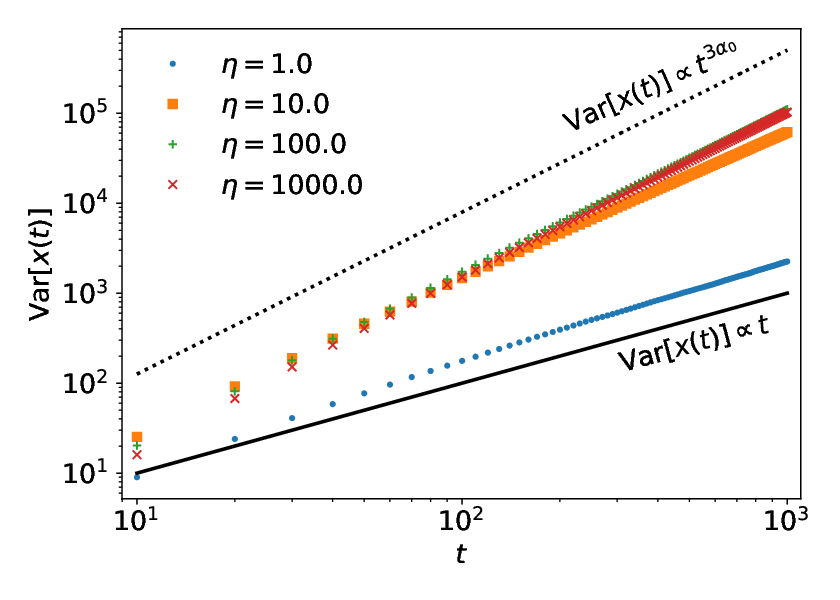

In this section, we validate the theoretical result in (20) and show the displacement PDFs as we vary . The numerical simulations for a single random walk corresponding to Eq. (4) were performed as follows:
- 1.
Initialize variables for current simulation time , particle position and current particle state . In this case, there are only three possible values for or corresponding to the rest, positive velocity and negative velocity states respectively. For simplicity, we assume the random walk starts in the positive velocity state.
- 2.
Initialize the constants of the simulation: , , , , and , the end time of simulation.
- 3.
If , generate a random number , where is a uniformly distributed random number. If , generate a random number .
- 4.
Increment the current simulation time and the particle position .
- 5.
If , set . If , generate a uniformly distributed random number, and calculate . For , set . For set . Otherwise, set. .
- 6.
Iterate steps 3 to 5 until .
The numerical simulations in this paper was performed using Python3 taking advantage of the ‘Numba’ package for JIT compilation and the ‘multiprocessing’ package for CPU parallelization. These packages were used to significantly improve simulation execution times.
Figures 2 and 3 show the emergence of superdiffusion and excellent correspondence with (20). Figure 4 shows the behavior of the PDF as the value of is varied. Clearly, when the rests become negligible in the asymptotic limit (), the drift of particles caused by self-reinforced directionality dominates. This clearly shows that particles engage in self-reinforcing directionality as rest states become less time consuming and particles choose to move in the same direction as their past history.
V Conclusion
In this paper, we have formulated a run-and-tumble model with self-reinforcing directionality and rests. The system of PDEs (4) has been reduced to a single, non-local equation for the total probability density (13). From this single governing equation, we demonstrated the emergence of superdiffusion by deriving the second moment for the long time limit. This emergence depends on two parameters: the self-reinforcement of particles, , and the ratio between running and resting rates, . We find that at the critical point, , superdiffusion emerges and remains for . In other words, the mean running time must be at least of the mean resting time for superdiffusion to occur in this model. Interestingly, we find that even a rest state cannot completely destroy the superdiffusion generated by self-reinforcement. Further, we present the method for Monte Carlo simulation of these random walks and show that the second moment corresponds with theoretical predictions. A natural extension of introducing resting times distributed with constant rate is to introduce a rest state that is non-Markovian with resting times distributed with a residence time dependent rate. This will generate power-law distributed resting times and is a well-known way to introduce subdiffusion in alternating systems Fedotov et al. 2010; Fedotov et al. 2011. It would interesting to find out if this destroys superdiffusion. It is also interesting to consider the case when the velocities alternate at non-exponentially distributed random times Di Crescenzo 2001 or driven by random trials Crimaldi et al. 2013. Furthermore, this new framework opens new avenues to include interactions of particles by density dependent rates, and , and velocity, , leading to aggregation and pattern formation in active matter Bechinger et al. 2016.
Acknowledgements.
S.F is thankful for the support and hospitality of the Ural Mathematical Center at the Ural Federal University, Ekaterinburg. SF also acknowledges financial support from RSF project 20-61-46013. D.H. acknowledges the support from Wellcome Trust Grant No. 215189/Z/19/Z. A.O.I. acknowledges financial support from the Ministry of Science and Higher Education of the Russian Federation (Ural Mathematical Center Project No. 075-02-2021-1387). D.H and M.A.A.S acknowledge financial support from FAPESP/SPRINT Grant No. 15308-4.References
- Hillen (2002) T. Hillen, Mathematical Models and Methods in Applied Sciences 12, 1007 (2002).
- Dolak and Hillen (2003) Y. Dolak and T. Hillen, Journal of mathematical biology 46, 153 (2003).
- Erban and Othmer (2004) R. Erban and H. G. Othmer, SIAM Journal on Applied Mathematics 65, 361 (2004).
- Filbet et al. (2005) F. Filbet, P. Laurençot, and B. Perthame, Journal of Mathematical Biology 50, 189 (2005).
- Bénichou et al. (2011) O. Bénichou, C. Loverdo, M. Moreau, and R. Voituriez, Reviews of Modern Physics 83, 81 (2011).
- Méndez et al. (2016) V. Méndez, D. Campos, and F. Bartumeus, Stochastic foundations in movement ecology (Springer, 2016).
- Angelani et al. (2014) L. Angelani, R. Di Leonardo, and M. Paoluzzi, The European Physical Journal E 37, 59 (2014).
- Bressloff and Newby (2013) P. C. Bressloff and J. M. Newby, Reviews of Modern Physics 85, 135 (2013).
- Selmeczi et al. (2005) D. Selmeczi, S. Mosler, P. H. Hagedorn, N. B. Larsen, and H. Flyvbjerg, Biophysical journal 89, 912 (2005).
- Othmer et al. (1988) H. G. Othmer, S. R. Dunbar, and W. Alt, Journal of Mathematical Biology 26, 263 (1988).
- Ridley et al. (2003) A. J. Ridley, M. A. Schwartz, K. Burridge, R. A. Firtel, M. H. Ginsberg, G. Borisy, J. T. Parsons, and A. R. Horwitz, Science 302, 1704 (2003).
- Tailleur and Cates (2008) J. Tailleur and M. Cates, Physical review letters 100, 218103 (2008).
- Bechinger et al. (2016) C. Bechinger, R. Di Leonardo, H. Löwen, C. Reichhardt, G. Volpe, and G. Volpe, Reviews of Modern Physics 88, 045006 (2016).
- Mendez et al. (2010) V. Mendez, S. Fedotov, and W. Horsthemke, Reaction-transport systems: mesoscopic foundations, fronts, and spatial instabilities (Springer Science & Business Media, 2010).
- Fetecau and Eftimie (2010) R. C. Fetecau and R. Eftimie, Journal of mathematical biology 61, 545 (2010).
- Thompson et al. (2011) A. G. Thompson, J. Tailleur, M. E. Cates, and R. A. Blythe, Journal of Statistical Mechanics: Theory and Experiment 2011, P02029 (2011).
- Farrell et al. (2012) F. Farrell, M. Marchetti, D. Marenduzzo, and J. Tailleur, Physical review letters 108, 248101 (2012).
- Carrillo et al. (2014) J. A. Carrillo, R. Eftimie, and F. K. Hoffmann, arXiv preprint arXiv:1407.2099 (2014).
- Stevens and Othmer (1997) A. Stevens and H. G. Othmer, SIAM Journal on Applied Mathematics 57, 1044 (1997).
- Huda et al. (2018) S. Huda, B. Weigelin, K. Wolf, K. V. Tretiakov, K. Polev, G. Wilk, M. Iwasa, F. S. Emami, J. W. Narojczyk, M. Banaszak, et al., Nature communications 9, 1 (2018).
- Fedotov (2016) S. Fedotov, Physical Review E 93, 020101 (R) (2016).
- Zaburdaev et al. (2015) V. Zaburdaev, S. Denisov, and J. Klafter, Reviews of Modern Physics 87, 483 (2015).
- Estrada-Rodriguez and Perthame (2021) G. Estrada-Rodriguez and B. Perthame, arXiv preprint arXiv:2109.08981 (2021).
- Taylor-King et al. (2016) J. P. Taylor-King, R. Klages, S. Fedotov, and R. A. Van Gorder, Physical Review E 94, 012104 (2016).
- Shaebani and Rieger (2019) M. R. Shaebani and H. Rieger, Frontiers in Physics 7, 120 (2019).
- Giona et al. (2019) M. Giona, M. D’Ovidio, D. Cocco, A. Cairoli, and R. Klages, Journal of Physics A: Mathematical and Theoretical 52, 384001 (2019).
- Wang et al. (2020) W. Wang, M. Höll, and E. Barkai, Physical Review E 102, 052115 (2020).
- Fedotov and Korabel (2017) S. Fedotov and N. Korabel, Physical Review E 95, 030107 (R) (2017).
- Han et al. (2021) D. Han, M. A. da Silva, N. Korabel, and S. Fedotov, Physical Review E 103, 022132 (2021).
- Schütz and Trimper (2004) G. M. Schütz and S. Trimper, Physical Review E 70, 045101 (R) (2004).
- da Silva et al. (2014) M. da Silva, G. Viswanathan, and J. Cressoni, Physical Review E 89, 052110 (2014).
- Boyer and Romo-Cruz (2014) D. Boyer and J. Romo-Cruz, Physical Review E 90, 042136 (2014).
- Baur and Bertoin (2016) E. Baur and J. Bertoin, Physical review E 94, 052134 (2016).
- Bercu et al. (2019) B. Bercu, M.-L. Chabanol, and J.-J. Ruch, Journal of Mathematical Analysis and Applications 480, 123360 (2019).
- Bercu and Laulin (2019) B. Bercu and L. Laulin, Journal of Statistical Physics 175, 1146 (2019).
- da Silva et al. (2020) M. da Silva, E. Rocha, J. Cressoni, L. da Silva, and G. Viswanathan, Physica A: Statistical Mechanics and its Applications 538, 122793 (2020).
- Mashanova et al. (2010) A. Mashanova, T. H. Oliver, and V. A. Jansen, Journal of the Royal Society Interface 7, 199 (2010).
- Tilles et al. (2016) P. F. Tilles, S. V. Petrovskii, and P. L. Natti, Royal Society open science 3, 160566 (2016).
- Klafter and Zumofen (1994) J. Klafter and G. Zumofen, Physical Review E 49, 4873 (1994).
- Zaburdaev and Chukbar (2002) V. Y. Zaburdaev and K. Chukbar, Journal of experimental and theoretical physics 94, 252 (2002).
- Klafter and Sokolov (2011) J. Klafter and I. M. Sokolov, First steps in random walks: from tools to applications (Oxford University Press, 2011).
- Portillo et al. (2011) I. G. Portillo, D. Campos, and V. Méndez, Journal of Statistical Mechanics: Theory and Experiment 2011, P02033 (2011).
- Fedotov et al. (2015) S. Fedotov, A. Tan, and A. Zubarev, Physical Review E 91, 042124 (2015).
- Fedotov et al. (2010) S. Fedotov, H. Al-Shamsi, A. Ivanov, and A. Zubarev, Physical Review E 82, 041103 (2010).
- Fedotov et al. (2011) S. Fedotov, A. Iomin, and L. Ryashko, Physical Review E 84, 061131 (2011).
- Di Crescenzo (2001) A. Di Crescenzo, Advances in Applied Probability 33, 690 (2001).
- Crimaldi et al. (2013) I. Crimaldi, A. Di Crescenzo, A. Iuliano, and B. Martinucci, Advances in applied probability 45, 1111 (2013).