Calibrated decoders for experimental quantum error correctionPreprint: APS/123-QED
Abstract
Arbitrarily long quantum computations require quantum memories that can be repeatedly measured without being corrupted. Here, we preserve the state of a quantum memory, notably with the additional use of flagged error events. All error events were extracted using fast, mid-circuit measurements and resets of the physical qubits. Among the error decoders we considered, we introduce a perfect matching decoder that was calibrated from measurements containing up to size-4 correlated events. To compare the decoders, we used a partial post-selection scheme shown to retain ten times more data than full post-selection. We observed logical errors per round of (decoded without post-selection) and (full post-selection), which was less than the physical measurement error of and therefore surpasses a pseudo-threshold for repeated logical measurements.
Keywords:
Quantum Information Processing, Quantum Memories, Quantum Correlations, Quantum Error Correction, Quantum ProtocolsI Introduction
Preparing and preserving logical quantum states is necessary for performing long quantum computations Gouzien and Sangouard 2021. Because noise inevitably corrupts the underlying physical qubits, quantum error correction (QEC) codes have been designed to detect and recover from errors Aharonov and Ben-Or 2008; Knill et al. 1996; Gottesman 1997; Shor 1995; Knill and Laflamme 1997. Significant efforts are currently focused on demonstrating capabilities that will be necessary for implementing practical QEC. An optimal choice of a code varies depending on the device and its noise properties Iyer and Poulin 2018. Notable experimental implementations include NMR Moussa et al. 2011; Zhang et al. 2011, ion traps Nigg et al. 2014; Linke et al. 2017; Egan et al. 2021; Ryan-Anderson et al. 2021, donors Waldherr et al. 2014; Abobeih et al. 2021; Hill et al. 2021, quantum dots Xue et al. 2021; Andrews et al. 2019, and superconducting qubits Reed et al. 2012; Kelly et al. 2015; Córcoles et al. 2015; Ristè et al. 2015; Takita et al. 2017. Recent developments of high-fidelity mid-circuit measurements and resets of superconducting qubits have enabled the preparation and repeated stabilization of logical states Andersen et al. 2020; Marques et al. 2021; Google Quantum AI 2021; demonstrations of such quantum memories with enhanced lifetimes have been limited by, among other reasons, a combination of gate and measurement cross-talk.
One way to mitigate cross-talk Takita et al. 2016 is to reduce the lattice connectivity Hertzberg et al. 2021; IBM Quantum 2020. Consequently, fault-tolerant operations require intermediary qubits; such qubits can be used to flag high-weight errors originating from low-weight errors Chao and Reichardt 2018; Chamberland and Beverland 2018. In certain QEC codes and lattice geometries, flag qubits supply the information needed to extend the effective distance of a QEC code up to its intended distance, and thus enable maximal efficiency at detecting and correcting errors Chamberland et al. 2020.

We demonstrated repeated error detection and correction of a error-detecting topological stabilizer code on a heavy-hexagonal (HH) device designed to mitigate the limiting effects of cross-talk using flag qubits. The combination of fast readout with reduced qubit connectivity improved, after post-selecting on instances in which no errors were detected, logical errors per round when compared to the physical measurement error rate. A thorough analysis of this code led us to introduce a partial post-selection scheme allowing us to discard ten times less data for comparing matching decoding algorithms. Compared against previously known decoding strategies on the entire data set, we found that a decoder performed best with experimentally-calibrated edge weights that account for the correlations between syndromes. Furthermore, we showed that correlations between five or more syndromes can be eliminated by the application of a “deflagging” procedure. The minimal impact of deflagging on logical errors is an encouraging sign that this technique, and its extension to general flag-based codes, is a viable way to process flag outcomes in practice.
II Theory

Active error-correction involves decoding, using syndrome measurements, the errors that occurred in the circuit so that the proper corrections can be applied. We define error-sensitive events to be linear combinations of syndrome measurement bits that, in an ideal circuit, would be zero. Thus, a non-zero error-sensitive event indicates some error has occurred. For the HH code, there are two types of error-sensitive events (1) the difference of two subsequent measurements of the same stabilizer, and (2) flag qubit measurements.
Error-sensitive events are depicted as nodes in a decoding graph with edges representing errors that are detected by both events at their end points (Fig. 2(a)). If the probability an edge occurs is , then the edge is given weight . The decoding graph may also have a boundary node, so that an error detected by just one error-sensitive event can be represented as an edge from that event to the boundary node. In practice, there are also errors detected by more than two error-sensitive events that could be represented as hyperedges in a more general decoding hypergraph.
Given a set of non-zero error-sensitive events, minimum-weight perfect-matching (MWPM) finds paths of edges connecting pairs of those events with minimum total weight, and is a simple and effective decoding algorithm for a topological stabilizer code that only operates on a decoding graph Higgott 2021, as opposed to a decoding hypergraph. While MWPM is computationally efficient, the analogous matching algorithm on a hypergraph is not, which limits the practicality of a decoding hypergraph.
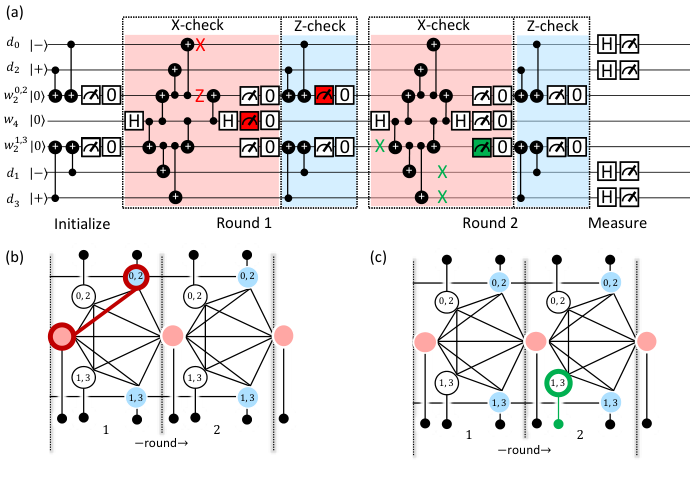
The effectiveness of MWPM depends crucially on edge weights in the decoding graph. We explored three strategies for setting these edge weights: (1) In the uniform approach, all edge weights were identical. (2) In the analytical approach, edge weights were individually calculated in terms of Pauli error rate parameters , where the index indicates one of the six errors being considered: CNOT gates, single-qubit gates, idle locations, initialization, resets, and measurements. The numerical values of the parameters can be chosen in several ways as discussed in Sect. III. (3) In the correlation approach, we analyzed experimental data to determine a set of edge probabilities that are likely to have produced it. This approach involved first calculating the probabilities for all hyperedges in the decoding hypergraph before determining the edge probabilities used in the decoder graph.
A hyperedge in the decoding hypergraph represents any of a number of Pauli faults in the circuit that are indistinguishable from one another because they each lead to the same set of non-zero error-sensitive events. If several faults occur together, the symmetric difference of their hyperedges is denoted , the syndrome, or, in other words, the set of non-zero error-sensitive events that is observed. The probability we observe a particular is the probability that hyperedges occur in combination to produce . Since this is related to the probability of an individual hyperedge occurring, we can learn from many observations of .
Realistically, the possible hyperedges are limited in size by locality of the circuits. In the code, we found that hyperedges are limited to sizes four or less. Finding in practical time begins by considering local clusters and then adjusting local estimates recursively from size-4 hyperedges down to size-1 and -2 (Fig. 2 and Supp. IV.7 Correlation analysis). Only size-1 and -2 edges are required for MWPM, but ignoring larger hyperedges can result in nonphysical, negative size-1 correlations.
Another way we explored decoding strategies was to consider analyzing only a subset of all data. By Pauli tracing (Supp. IV.4 Pauli fault tracing), we classified edges in the decoding graph into three categories depending on whether its inclusion in the minimum-weight matching necessitated: (1) flipping the logical measurement, (2) not flipping the logical measurement, or (3) is ambiguous (Fig. S1). The ambiguous case occurs specifically for error-detecting codes, like the code presented here, because some errors result in the decoder having to choose between two equally probable corrections.
Using these classifications for edges in the decoder graph, we explored three degrees of post-selection. The most conservative approach, using full post-selection, involved discarding all results showing any non-zero error-sensitive event; this approach was the only one in which further decoding cannot be done. In the opposite regime, without post-selection, all results were kept and any ambiguous edges in the MWPM were treated without flipping the logical measurement; here, logical error rates could have been improved by decoding but was not strictly needed. Finally, the intermediate regime involved a partial post-selection scheme whereby results were only discarded if the MWPM algorithm highlighted an ambiguous edge; here, decoding had to be done so that results with ambiguous edges that were highlighted could be discarded.

III Experimental results
Fitting the adjusted hyperedge probabilities to analytical expressions produces approximate estimates for the six-noise parameters in the error correcting experiments (Fig. 2(b)). These noise estimates were found to be in good agreement with benchmarks based on simultaneous randomized benchmarking. Experiments were performed on four logical states ( and ) each of which was stabilized up to 10 rounds to extract a logical error per round of stabilizers (Fig. 3). This logical error varied depending on the analysis method.
For the full post-selection scheme, the logical error for some rounds fell below the best and average physical initialization and measurement errors - a hallmark of being below a so-called pseudo-threshold for fault-tolerant quantum computing. Fitting the decay curves resulted in inferred logical errors per round of for , and for .
If none of the instances of the experiment were discarded, then the logical error remained consistently above the pseudo-threshold. In this analysis without any post-selection and without decoding, we inferred logical errors per round of for , and for .
Recalling that the is an error detecting code, we used the syndrome outcomes from each stabilizer round to perform a post-facto logical correction in software. Discarding instances where ambiguous edges were highlighted by the decoder allowed us to apply the partial, in contrast with the full, post-selection scheme. With this scheme, significantly more instances of the experimental runs remained, resulting in inferred logical errors per round of for , and for .

Within the none and partial post-selection schemes, we were able to compare the performance of three different instances of decoders (Fig. 4). The most generic decoder assumes there was no known noise model for the underlying physical system. Such a uniform decoder graph, in which every edge of the decoder graph was given equal weights, was expected to perform better than no decoding at all; but, was expected to be worse than any other graph whose edges were informed by some knowledge of the underlying noise. For instance, by selecting a simple, Pauli noise model, analytical expressions for the edge weights were calculated and led to improved logical error rates. Alternatively, if no assumptions were made about the noise, then edge weights were populated by the experimentally calibrated, correlation probabilities described earlier. We found that, as expected, such a correlation decoder graph indeed corrected for logical errors more effectively than the uniform decoding strategy and compared well with the analytical method (Fig. 4(b)). However, when the partial post-selection scheme was used, this trend no longer held since an analytical decoder with noise parameters from simultaneous randomized benchmarking outperformed the correlation analysis (Fig. 4(c)).
While the correlation analysis should, in principle, contain complete information about all of the noise in our experiments, its implementation is expected to become more computationally costly when applied to codes at larger distances. We simplified the decoder graph, and thus the number and size of hyperedges needed in the correlation analysis, by feeding-forward information from each round of flag measurements. This procedure, known as “deflagging” (Supp. IV.6 Deflagging procedure), allowed us to eliminate all 30 of the size-4 hyperedges in an experiment with 10 rounds of stabilizer measurements without a significant increase in the logical error per round (Fig. 4). Furthermore, the logical errors were mostly preserved compared to results without the deflagging procedure.
Naiv̈ely extending the HH code to distance-3 would result in size-5 hyperedges arising in the decoder hypergraph. However, when deflagging is applied, we found that there were no longer any size-5 hyperedges, and the number of size-4 hyperedges reduced from to , where is the number of rounds. Since the computational resources scale exponentially with the largest weight hyperedge in a graph, we expect that the deflagging procedure will provide a dramatic reduction in the computational resources needed to carry out the correlation analysis for codes beyond distance-3.
IV Conclusion
Experimentally preparing and repeatedly stabilizing a logical quantum state, with error rates nearly ten times smaller than the lowest physical measurement error rate, is an important step towards executing larger, fault-tolerant circuits. The hexagonal lattice on which we demonstrated our findings can be extended to operate larger distance versions of the fault-tolerant HH code used here, or for other related codes Hastings and Haah 2021; Gidney et al. 2021; Wootton 2021. Although the distance-2 version was implemented on a subset of qubits within a hexagonal lattice, other topologies are also expected to benefit; for example, a heavy-square topology akin to the rotated surface code with added flag qubits Chamberland et al. 2020. Nevertheless, our probabilistic error correction methods and higher order error correlation analysis represents an approach for improving decoders for codes with or without flags within any device topology. We also demonstrated an effective use of flags to limit the extent of the correlations needed for efficient decoding. Our approach for extracting quantitative noise figures from the experiments creates a path to diagnose and reduce the logical errors per round of codes at larger distances.
As quantum computing devices become larger and less noisy, approaches such as ours may form the basis for efficiently decoding experimentally relevant errors. Other decoding strategies such as maximum-likelihood algorithms are known to scale unfavorably with code distances but may also benefit from our approach Bravyi et al. 2014; Bravyi and Cross 2015; Heim et al. 2016. Eventually, decoders will need to be trained in real-time Das et al. 2021, whereby logical operations could be interleaved with calibration circuits to periodically update the decoder graph’s prior information with calibrated correlation probabilities. Previously studied bootstrapping techniques Google Quantum AI 2021 coupled with the periodic re-calibration of the correlation edges may eventually approach near-optimal decoding efficiencies, although the existence of an optimal strategy remains an open question.
References
- Gouzien and Sangouard (2021) É. Gouzien and N. Sangouard, Factoring 2048-bit RSA Integers in 177 Days with 13 436 Qubits and a Multimode Memory, Physical Review Letters 127, 140503 (2021).
- Aharonov and Ben-Or (2008) D. Aharonov and M. Ben-Or, Fault-Tolerant Quantum Computation with Constant Error Rate, SIAM Journal on Computing 38, 1207 (2008).
- Knill et al. (1996) E. Knill, R. Laflamme, and W. Zurek, Threshold Accuracy for Quantum Computation, arXiv:quant-ph/9610011 (1996), arXiv:quant-ph/9610011 .
- Gottesman (1997) D. Gottesman, Stabilizer Codes and Quantum Error Correction (California Institute of Technology, 1997).
- Shor (1995) P. W. Shor, Scheme for reducing decoherence in quantum computer memory, Physical review A 52, R2493 (1995).
- Knill and Laflamme (1997) E. Knill and R. Laflamme, Theory of quantum error-correcting codes, Physical Review A 55, 900 (1997).
- Iyer and Poulin (2018) P. Iyer and D. Poulin, A small quantum computer is needed to optimize fault-tolerant protocols, Quantum Science and Technology 3, 030504 (2018).
- Moussa et al. (2011) O. Moussa, J. Baugh, C. A. Ryan, and R. Laflamme, Demonstration of Sufficient Control for Two Rounds of Quantum Error Correction in a Solid State Ensemble Quantum Information Processor, Physical Review Letters 107, 10.1103/PhysRevLett.107.160501 (2011).
- Zhang et al. (2011) J. Zhang, D. Gangloff, O. Moussa, and R. Laflamme, Experimental quantum error correction with high fidelity, Physical Review A 84, 034303 (2011).
- Nigg et al. (2014) D. Nigg, M. Müller, E. A. Martinez, P. Schindler, M. Hennrich, T. Monz, M. A. Martin-Delgado, and R. Blatt, Quantum computations on a topologically encoded qubit, Science 345, 302 (2014).
- Linke et al. (2017) N. M. Linke, M. Gutierrez, K. A. Landsman, C. Figgatt, S. Debnath, K. R. Brown, and C. Monroe, Fault-tolerant quantum error detection, Science advances 3, e1701074 (2017).
- Egan et al. (2021) L. Egan, D. M. Debroy, C. Noel, A. Risinger, D. Zhu, D. Biswas, M. Newman, M. Li, K. R. Brown, M. Cetina, and C. Monroe, Fault-tolerant control of an error-corrected qubit, Nature , 1 (2021).
- Ryan-Anderson et al. (2021) C. Ryan-Anderson, J. G. Bohnet, K. Lee, D. Gresh, A. Hankin, J. P. Gaebler, D. Francois, A. Chernoguzov, D. Lucchetti, N. C. Brown, T. M. Gatterman, S. K. Halit, K. Gilmore, J. Gerber, B. Neyenhuis, D. Hayes, and R. P. Stutz, Realization of real-time fault-tolerant quantum error correction, arXiv:2107.07505 [quant-ph] (2021), arXiv:2107.07505 [quant-ph] .
- Waldherr et al. (2014) G. Waldherr, Y. Wang, S. Zaiser, M. Jamali, T. Schulte-Herbrüggen, H. Abe, T. Ohshima, J. Isoya, J. F. Du, P. Neumann, and J. Wrachtrup, Quantum error correction in a solid-state hybrid spin register, Nature 10.1038/nature12919 (2014).
- Abobeih et al. (2021) M. H. Abobeih, Y. Wang, J. Randall, S. J. H. Loenen, C. E. Bradley, M. Markham, D. J. Twitchen, B. M. Terhal, and T. H. Taminiau, Fault-tolerant operation of a logical qubit in a diamond quantum processor, arXiv:2108.01646 [cond-mat, physics:quant-ph] (2021), arXiv:2108.01646 [cond-mat, physics:quant-ph] .
- Hill et al. (2021) C. D. Hill, M. Usman, and L. C. L. Hollenberg, An exchange-based surface-code quantum computer architecture in silicon, arXiv:2107.11981 [cond-mat, physics:physics, physics:quant-ph] (2021), arXiv:2107.11981 [cond-mat, physics:physics, physics:quant-ph] .
- Xue et al. (2021) X. Xue, M. Russ, N. Samkharadze, B. Undseth, A. Sammak, G. Scappucci, and L. M. K. Vandersypen, Computing with spin qubits at the surface code error threshold, arXiv:2107.00628 [cond-mat, physics:quant-ph] (2021), arXiv:2107.00628 [cond-mat, physics:quant-ph] .
- Andrews et al. (2019) R. W. Andrews, C. Jones, M. D. Reed, A. M. Jones, S. D. Ha, M. P. Jura, J. Kerckhoff, M. Levendorf, S. Meenehan, S. T. Merkel, A. Smith, B. Sun, A. J. Weinstein, M. T. Rakher, T. D. Ladd, and M. G. Borselli, Quantifying error and leakage in an encoded Si/SiGe triple-dot qubit, Nature Nanotechnology 14, 747 (2019).
- Reed et al. (2012) M. D. Reed, L. DiCarlo, S. E. Nigg, L. Sun, L. Frunzio, S. M. Girvin, and R. J. Schoelkopf, Realization of three-qubit quantum error correction with superconducting circuits, Nature 482, 382 (2012).
- Kelly et al. (2015) J. Kelly, R. Barends, A. G. Fowler, A. Megrant, E. Jeffrey, T. C. White, D. Sank, J. Y. Mutus, B. Campbell, Y. Chen, Z. Chen, B. Chiaro, A. Dunsworth, I.-C. Hoi, C. Neill, P. J. J. O’Malley, C. Quintana, P. Roushan, A. Vainsencher, J. Wenner, A. N. Cleland, and J. M. Martinis, State preservation by repetitive error detection in a superconducting quantum circuit, Nature 519, 66 (2015).
- Córcoles et al. (2015) A. D. Córcoles, E. Magesan, S. J. Srinivasan, A. W. Cross, M. Steffen, J. M. Gambetta, and J. M. Chow, Demonstration of a quantum error detection code using a square lattice of four superconducting qubits, Nature Communications 6, 6979 (2015).
- Ristè et al. (2015) D. Ristè, S. Poletto, M.-Z. Huang, A. Bruno, V. Vesterinen, O.-P. Saira, and L. DiCarlo, Detecting bit-flip errors in a logical qubit using stabilizer measurements, Nature Communications 6, 6983 (2015).
- Takita et al. (2017) M. Takita, A. W. Cross, A. D. Córcoles, J. M. Chow, and J. M. Gambetta, Experimental Demonstration of Fault-Tolerant State Preparation with Superconducting Qubits, Physical Review Letters 119, 180501 (2017).
- Andersen et al. (2020) C. K. Andersen, A. Remm, S. Lazar, S. Krinner, N. Lacroix, G. J. Norris, M. Gabureac, C. Eichler, and A. Wallraff, Repeated quantum error detection in a surface code, Nature Physics 16, 875 (2020).
- Marques et al. (2021) J. F. Marques, B. M. Varbanov, M. S. Moreira, H. Ali, N. Muthusubramanian, C. Zachariadis, F. Battistel, M. Beekman, N. Haider, W. Vlothuizen, A. Bruno, B. M. Terhal, and L. DiCarlo, Logical-qubit operations in an error-detecting surface code, arXiv:2102.13071 [cond-mat, physics:quant-ph] (2021), arXiv:2102.13071 [cond-mat, physics:quant-ph] .
- Google Quantum AI (2021) Google Quantum AI, Exponential suppression of bit or phase errors with cyclic error correction, Nature 595, 383 (2021).
- Takita et al. (2016) M. Takita, A. D. Córcoles, E. Magesan, B. Abdo, M. Brink, A. Cross, J. M. Chow, and J. M. Gambetta, Demonstration of Weight-Four Parity Measurements in the Surface Code Architecture, Physical Review Letters 117, 210505 (2016).
- Hertzberg et al. (2021) J. B. Hertzberg, E. J. Zhang, S. Rosenblatt, E. Magesan, J. A. Smolin, J.-B. Yau, V. P. Adiga, M. Sandberg, M. Brink, J. M. Chow, and J. S. Orcutt, Laser-annealing Josephson junctions for yielding scaled-up superconducting quantum processors, npj Quantum Information 7, 1 (2021).
- IBM Quantum (2020) IBM Quantum, High-fidelity superconducting quantum processors via laser-annealing of transmon qubits, arXiv:2012.08475 [quant-ph] (2020), arXiv:2012.08475 [quant-ph] .
- Chao and Reichardt (2018) R. Chao and B. W. Reichardt, Quantum Error Correction with Only Two Extra Qubits, Physical Review Letters 121, 050502 (2018).
- Chamberland and Beverland (2018) C. Chamberland and M. E. Beverland, Flag fault-tolerant error correction with arbitrary distance codes, Quantum 2, 53 (2018).
- Chamberland et al. (2020) C. Chamberland, G. Zhu, T. J. Yoder, J. B. Hertzberg, and A. W. Cross, Topological and subsystem codes on low-degree graphs with flag qubits, Physical Review X 10, 011022 (2020), arXiv:1907.09528 .
- Higgott (2021) O. Higgott, PyMatching: A Python package for decoding quantum codes with minimum-weight perfect matching, arXiv:2105.13082 [quant-ph] (2021), arXiv:2105.13082 [quant-ph] .
- Hastings and Haah (2021) M. B. Hastings and J. Haah, Dynamically Generated Logical Qubits, arXiv:2107.02194 [quant-ph] (2021), arXiv:2107.02194 [quant-ph] .
- Gidney et al. (2021) C. Gidney, M. Newman, A. Fowler, and M. Broughton, A Fault-Tolerant Honeycomb Memory, arXiv:2108.10457 [quant-ph] (2021), arXiv:2108.10457 [quant-ph] .
- Wootton (2021) J. R. Wootton, Hexagonal matching codes with 2-body measurements, arXiv:2109.13308 [quant-ph] (2021), arXiv:2109.13308 [quant-ph] .
- Bravyi et al. (2014) S. Bravyi, M. Suchara, and A. Vargo, Efficient Algorithms for Maximum Likelihood Decoding in the Surface Code, Physical Review A 90, 032326 (2014), arXiv:1405.4883 .
- Bravyi and Cross (2015) S. Bravyi and A. Cross, Doubled Color Codes, arXiv:1509.03239 [quant-ph] (2015), arXiv:1509.03239 [quant-ph] .
- Heim et al. (2016) B. Heim, K. M. Svore, and M. B. Hastings, Optimal Circuit-Level Decoding for Surface Codes, arXiv:1609.06373 [quant-ph] (2016), arXiv:1609.06373 [quant-ph] .
- Das et al. (2021) P. Das, A. Locharla, and C. Jones, LILLIPUT: A Lightweight Low-Latency Lookup-Table Based Decoder for Near-term Quantum Error Correction, arXiv:2108.06569 [quant-ph] (2021), arXiv:2108.06569 [quant-ph] .
- IBM Quantum and Community (2021) IBM Quantum and Community, Qiskit: An open-source framework for quantum computing (2021).
- Bravyi et al. (2021) S. Bravyi, S. Sheldon, A. Kandala, D. C. Mckay, and J. M. Gambetta, Mitigating measurement errors in multiqubit experiments, Physical Review A 103, 042605 (2021).
- Garion et al. (2021) S. Garion, N. Kanazawa, H. Landa, D. C. McKay, S. Sheldon, A. W. Cross, and C. J. Wood, Experimental implementation of non-Clifford interleaved randomized benchmarking with a controlled-$S$ gate, Physical Review Research 3, 013204 (2021).
- (44) C. Gidney, Decorrelated depolarization, https://algassert.com/post/2001 (2020), accessed:2021-08-23.
- Chao et al. (2020) R. Chao, M. E. Beverland, N. Delfosse, and J. Haah, Optimization of the surface code design for Majorana-based qubits, Quantum 4, 352 (2020).
- Sundaresan et al. (2020) N. Sundaresan, I. Lauer, E. Pritchett, E. Magesan, P. Jurcevic, and J. M. Gambetta, Reducing Unitary and Spectator Errors in Cross Resonance with Optimized Rotary Echoes, PRX Quantum 1, 020318 (2020).
- Blais et al. (2004) A. Blais, R.-S. Huang, A. Wallraff, S. M. Girvin, and R. J. Schoelkopf, Cavity quantum electrodynamics for superconducting electrical circuits: An architecture for quantum computation, Physical Review A 69, 062320 (2004).
- Córcoles et al. (2021) A. D. Córcoles, M. Takita, K. Inoue, S. Lekuch, Z. K. Minev, J. M. Chow, and J. M. Gambetta, Exploiting Dynamic Quantum Circuits in a Quantum Algorithm with Superconducting Qubits, Physical Review Letters 127, 100501 (2021).
Acknowledgements.
We wish to acknowledge Ben W. Reichardt (USC) for proposing the deflagging procedure, Joe Latone for discussions on optimizing the numerical analysis, Ted Thorbeck for initial suggestions on readout tune-up, David Lokken-Toyli and Oliver Dial for discussions on characterizing measurement impact on qubit states, and Isaac Lauer, Andrew Eddins, David McKay and Sarah Sheldon for valuable discussions. These results were enabled by the work of the IBM Quantum software and hardware teams. We acknowledge support by IARPA under contract W911NF-16-1-0114 for the theoretical and experimental work (including partial device bring-up, characterization, and gate and measurement calibration) presented in this manuscript. The device was designed and fabricated internally at IBM. E.H.C. and T.J.Y. contributed equally to this work. M.L. and A.W.C. performed simulations and analysis. Y.K., N.S., S.S., A.D.C. and M.T. designed and conducted the experiments. All authors contributed to writing the manuscript.Supplementary Material
IV.1 Code preparation and measurement
Here we describe briefly how to prepare, maintain, and measure logical states of the code. A set of stabilizer generators for this code is
| (1) |
and its logical operators can be chosen as and , where the ordering of the Pauli operators on data qubits ‘0’ through ‘3’ are indexed from left to right. The stabilizer formalism implies logical states
| (2) | ||||
which are -eigenstates of , respectively. The -eigenstates of are and .
Rather than create these logical states via unitary evolution, which may spread errors in a non-fault-tolerant fashion, instead we use projective measurements. For example, the state is prepared beginning with the state , which is already a -eigenstate of , , and , and measuring using the X-check circuit from Fig. 1(c). Without circuit noise, if the measurement reports (-eigenstate), then we have prepared , and if it reports (-eigenstate), we have prepared . In the second case, we could obtain by applying to the last qubit, but instead we just flip all subsequent measurements of to account for it.
We likewise prepare by starting with and measuring , by starting with and measuring and , and by starting with and measuring and . Again, in each case, we may end up preparing a state that differs by a Pauli from the logical state we intended (there is one such case for or and three cases for or ), but this is accounted for by subsequently flipping the appropriate stabilizer measurements in the rest of the circuit.
After state preparation the circuit continues by repeated measurements of the stabilizers, alternating X- and Z-check circuits from Fig. 1. If the state preparation required measuring and (the and cases), then a “round” of syndrome measurement consists of the X-check circuit followed by the Z-check circuit. Alternatively, if the state preparation required measuring (the and cases), then a round of syndrome measurement consists of the Z-check circuit followed by the X-check circuit. The number of rounds is a parameter that we swept up to 10 in our experiments.
Following the rounds of syndrome measurements, all four code qubits are measured in the same basis. If we prepared states or they are measured in the -basis, and if we prepared or they are measured in the -basis. From this measurement information, the values of some stabilizers and one of the two logical operators ( or ) can be inferred.
See Fig. 1(c) for an example of the circuitry described in this section for the case.
IV.2 Summary of experiments
All experiments were taken with shots. In anticipation of executing larger distance codes on the heavy hexagon lattice, a variety of experimental configurations were explored:
- 1.
Code layouts
: and
: . - 2.
All 7 possible sets of 7 physical qubits needed for on the lattice of 27 qubits.
- 3.
Initial states , , , .
- 4.
Logical state definitions
vs. or
vs. - 5.
With and without dynamical decoupling during idling periods.
- 6.
Both (in main text) vs. single stabilizer measurement checks (i.e. only X-stabilizers in each round)
- 7.
With and without stabilizer measurement rounds of identical duration - showing that stabilizer checks preserved logical states with higher fidelity than simply idling the qubits.
IV.3 State tomography
Upon preparing the logical states using the projective protocol described in Supp. IV.1 Code preparation and measurement we performed quantum state tomography of the four data qubits. We used the methodology implemented in Qiskit Ignis (Qiskit version 0.23.0, Terra version 0.17.0, Ignis version 0.6.0) IBM Quantum and Community 2021 and ran measurement error mitigation Bravyi et al. 2021 in its full noise matrix variant also as offered in Ignis. The reconstructed 4-qubit density matrix was then used to compute the state fidelity as where is one of the logical states described in Eq. 2, or the equivalent logical states in the basis. We used the cvx method for state reconstruction in the StateTomographyFitter class (see Qiskit Ignis documentation for more details). We further projected the resulting 4-qubit density matrix onto the logical codespace Takita et al. 2017; Andersen et al. 2020; Marques et al. 2021 to obtain the logical codespace probability, , along with an acceptance probability, , as shown in Table S1.
Suppose we focus on the preparation of as an example. Without any errors, state tomography would give , where is the state expected after measuring ‘0’ for (namely, ) and is the state expected after measuring ‘1’ (namely, ). The state is an equal classical mixture of the two cases because they occur with equal probability. Now, define
| (3) | ||||
| (4) |
which represent the probabilities we have the expected logical state and the probability we are in the codespace, respectively. Note, is called the acceptance probability because it is bounded between ‘0’ and ‘1’.
The cases for , , and are analogous. It is worth noting that in the and cases, is the equal mixture of four states, corresponding to the four possible combinations of measurement outcomes for and . Also, in the and cases, we keep only those runs with trivial flag measurements, as non-trivial flag measurements means an error must have occurred.
For these state tomography experiments, we applied readout correction Bravyi et al. 2021 by constructing a noisy measurement basis from the readout calibration matrix whose projectors are then used in the state reconstruction, as detailed in Ref. Garion et al. 2021.
| logical state | |||
|---|---|---|---|
IV.4 Pauli fault tracing
A standard model of faults in quantum error-correction is Pauli depolarizing noise: any qubit initialization, gate, idle location, or measurement can suffer a fault, in which case it is followed (or preceded, in the case of a measurement) by a Pauli acting on the same number of qubits (1 or 2) as the circuit component. Initializations and measurements can just suffer errors (as errors have no effect), while 1- and 2-qubit gates can suffer any error from the 1- or 2-qubit Pauli groups.
Consider the set of Pauli errors that result from single faults in the syndrome measurement circuits. For each Pauli error in this set, propagate it through the circuit and determine the set of error-sensitive events that detect the error. This set becomes a hyperedge in the decoding hypergraph. At first order, the probability of that hyperedge is just the sum of probabilities of the faults that can cause it, and its hyperedge weight is . These hyperedges that can be predicted and categorized for partial post-selection and decoding are shown in Fig. S1.
Not all hyperedges in the graph end up having a probability assigned. For example, in real hardware computational leakage occurs and is not accounted for by the Pauli tracer; so hyperedges not predicted by the Pauli tracer can appear in experiments such as those in Fig. 2.

IV.5 Decoding examples
Some examples of how single Pauli faults can be used by a decoder. When certain edges are highlighted (Fig. S1), error correction is possible for certain Pauli errors (Fig. S2(b)) while others are not (Fig. S2(c)).
IV.6 Deflagging procedure
Using the deflagging procedure illustrated in Fig. S3, the largest hyperedge sizes in the decoder hypergraph can be shown, using the Pauli tracer in Supp. IV.4 Pauli fault tracing, to be of size no greater than 4 for the distance-3 HH code. Generalizations of this procedure to larger distances will be discussed in upcoming work.

IV.7 Correlation analysis
The goal of the correlation decoder is to learn hyperedge probabilities from a set of measurement data. To do so, we assume that hyperedges occur independently. While this is not strictly true in the standard model of depolarizing noise where faults are mutually exclusive (e.g. if a Hadamard gate fails with an error it cannot simultaneously fail with a error), it is easy enough to find an independent error model that is equivalent to the exclusive one (see 11 1 C. Gidney, Decorrelated depolarization, https://algassert.com/post/2001 (2020), accessed:2021-08-23. and Chao et al. 2020), justifying the assumption of independent hyperedges.
Denote the set of error-sensitive events by and the set of possible hyperedges by . One can determine from, for instance, Pauli tracing of single faults with additional hyperedges added if they are suspected to be of experimental relevance. From measurement data, one has access to estimates of the expectation values , where is the binary random variable associated to error-sensitive event and is a hyperedge. Also, these expectation values can be written in terms of hyperedge probabilities . Suppose is the set of hyperedges that have non-empty intersection with . Then we have
| (5) |
where denotes the symmetric difference of sets. Writing these equations for all , one in principle has a system of equations and unknowns that can be solved for in terms of the experimentally estimated expectations . In practice, this system of equations is too expensive to solve, even numerically, for . For instance, a experiment preserving the logical state for rounds of syndrome measurement has , which is already prohibitively large for .
Therefore, we must settle for an approximate solution to the equations. This proceeds as follows. First, cluster hyperedges by finding a subset (where is the powerset of ) such that for all , there is a such that . A simple approach for clustering is to sort hyperedges by size, from largest to smallest. Go through the sorted list, placing a hyperedge into if it is not already a subset of some element of . We refer to elements of as clusters. It is important for what follows that clusters are small, and it is evident from the prescribed clustering approach that the largest cluster size is equal to the largest hyperedge size.
Next, solve each cluster . Suppose is the set of hyperedges that are a subset of . For each , calculate as if are the only hyperedges that exist. That is,
| (6) |
Now we have a system of equations and unknowns, the for all . If clusters are small, this is fast to solve. In particular, a size-2 cluster can be solved analytically (see Google Quantum AI 2021), while clusters with sizes three and four can be solved numerically. In general, a cluster with size leads to at most equations.
The cluster solving procedure is approximate because clusters are solved assuming only hyperedges within them exist, while in actuality some hyperedges span different clusters. The final step is to adjust solutions based on these spanning hyperedges.
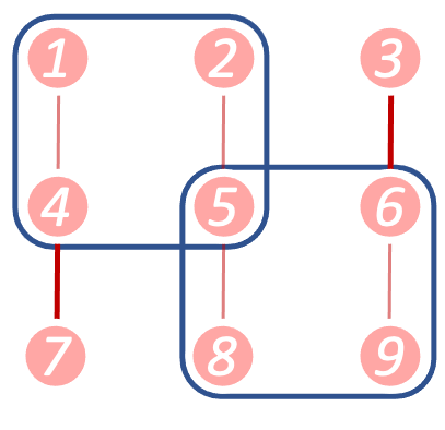
An example of the idea is the following (Fig. S4). Suppose is a hyperedge within cluster , which has some probability . Suppose another hyperedge exists, and but . When we solved cluster , we obtained some probability for hyperedge , but because we ignored , is actually the sum of two different events: either occurred without occurring, or occurred without occurring. Therefore, , and so is the probability of adjusted by . Adjustment commutes – if we need to adjust by several hyperedges, we can adjust by one at a time in any order.
Maximum-size hyperedges do not require adjustment, since there is no larger to adjust by, and they provide a base case for the recursive adjustment of all smaller size hyperedges. This proceeds as follows: (1) Adjust each hyperedge of size by finding all hyperedges with weight at least , such that and . (2) For all such , perform the update . After doing this for all we are left with an adjusted . (3) Finally, because might be in several different clusters, we might have multiple adjusted . Average the adjusted values to get a final .
We highlight a point of caution. If one executes step (1) not starting with the largest hyperedges in the graph with weight , but instead only with size-2 hyperedges (which was done for the repetition code in Google Quantum AI 2021), then one could arise at non-physical values for (Fig. S6).
In Fig. S5, we provide simulations that suggest the correlation analysis is providing an accurate assessment of the hyperedge probabilities. The error in the correlation analysis scales with the number of runs of the experiment, , as .


IV.8 Partial post-selection
To implement partial post-selection with the code, the edges highlighted by the MWPM decoding algorithm need to be compared against the three classes of edges classified in Fig. S1. The illustrated decoder graph will change depending on the logical state and the code layout. Also, the ambiguous edges do not appear for codes in cases with only single faults per round, and so such a partial post-selection scheme is no longer applicable in those cases.
IV.9 Device properties
Characterized noise properties of the 7 qubits used in ibmq_kolkata are shown in Table S3. All 1-qubit gates had a duration of 35.55 ns. The measurement pulse width and integration windows were approximately 330 ns. The total measurement and conditional reset cycling time, including delays from the cable transmission and electronic latency, were approximately 764 ns. Table S4 shows the result of optimizing the error per gate for each entangling, cross-resonance rotary echo gate Sundaresan et al. 2020. The direction of the cross-resonance gates were chosen to minimize the impact of spectator qubits. Composing these operations resulted in Z-(X-)stabilizer checks lasting for ().
IV.10 Calibration of measurement power
An optimal mid-circuit measurement tone needs to have sufficiently high power to distinguish the and states without inducing substantial measurement back-action. We optimized our mid-circuit measurement tones by utilizing the repeated measurement protocol illustrated in Fig. S7(a). The protocol involves preparing the state in a superposition of and using a pulse, and then concluding with two sequential readout pulses. The outcome of the first readout pulse should be random, while the second result should, ideally, match the first if the state was not impacted by measurement back-action or poor readout fidelity. We quantify the degree of measurement-induced back-action using the quantum non-demolition (QND) probability defined as
| (7) |
which tracks whether the state was unchanged from the previous measurement. However, excessive readout power can also result in excitations out of the computational basis and into leaked states, which can be incorrectly categorized as or by a linear state discriminator. To remedy this situation, we inserted a pulse which leaves non-computational states unchanged but induces a bit-flip if the state was within the computational basis. Thus, we define
| (8) |
which quantifies the computational leakage. Note that we also incorporated a delay pulse, , whose length was chosen to be , where ns was the measurement tone width and MHz is the median of the device. The additional time delay allows the cavity to depopulate and thus prevents errors when applying the subsequent operation. Figure S7(b) shows and as a function of the average cavity photon number normalized by the critical photon number Blais et al. 2004 in blue and red, respectively. In the expression above, is the qubit anharmonicity and is the cavity-qubit detuning. Three different DAC amplitudes were converted to average photon numbers using the protocol described in Ref. Córcoles et al. 2021 and the fitted curve was used for extrapolation. The particular critical photon number for this qubit was ( MHz, MHz, and GHz). When the cavity was populated with low photon numbers, both and curves showed monotonically increasing trends as the state distinguishability improved and, consequently, the readout error decreased. When we reached substantially high measurement powers, we observed a gradual degradation in compared with due to the population of the state. Note that was incorrectly recorded as and is not captured in the metric. However, applying a gate captures the transition to as an additional degradation in . The optimal photon number, or DAC amplitude, was thus chosen to maximize . The same procedure was repeated for all qubits as illustrated in Fig. S7(c) resulting in an overall average value for .

IV.11 Non-local effect of measurements
IV.11.1 Measurement-induced phase rotations
The multiple readout cavities were designed specifically to have frequencies and other operating parameters to allow for simultaneous readout from the same output line. However, due to variations in the fabrication process, cavity frequencies were, in this case, closer than intended. This resulted in phase rotations on data qubits induced by unintended coupling to nearby readout cavities. While we found no evidence of dephasing detected in two qubit pairs within the same readout multiplexed line, we observed coherent phase rotations between qubits on pairs of cavities whose readout frequency separations were smaller than intended.
As an egregious example of this effect, we chose a pair of qubits in a separate device whose readout frequencies turned up in practice closer than intended in design. This pair of qubits were coupled to readout cavities both coupled to the same, multiplexed line with frequencies MHz apart and therefore closer than intended. Fig. S8(a) shows an experiment for two qubits not on ibmq_kolkata where one qubit (Q1) is prepared with , and measured in all different axes projections, , after a fixed delay time . While monitoring Q1, we applied a probe measurement tone on another qubit, Q2 (M2). While we increased the probe measurement tone (M2), we observed coherent rotations on Q1, as seen on - and - projections. Note that the state vector length (black line) was relatively constant, indicating that there was no significant dephasing. We computed the rotation angles from - and - projections in Fig. S8(b) and inferred the photon number of the Q1 cavity by using an independently measured MHz. Fig. S8(c) shows that a fractional photon number was populated in the Q1 cavity, which caused an undesirable -rotation. This possible photon leakage may have induced a phase error on data qubits during syndrome measurements. Fortunately, this undesirable -rotation was corrected by inserting refocusing pulses. Fig. S8(d) illustrates the same experiment as (a) but with a dynamical decoupling sequence () inserted during the idling time. As a result, the measurement-induced -rotation was no longer observed. These experiments suggest that the improved logical error rates when dynamical decoupling is used can be explained by the suppression of undesirable, measurement-induced phase errors during the syndrome measurements.
IV.11.2 Measurement-induced collisions
Our readout resonators were designed to operate at GHz so that they operated above the qubit frequencies at GHz. In this frequency configuration, an applied measurement tone Stark-shifts the connected qubits lower in frequency. The qubits can unintentionally be Stark-shifted into resonance with an adjacent qubit causing measurement-induced collisions, which degrade the readout fidelity.
Although such an effect was not isolated on ibmq_kolkata, we observed this effect on a pair of qubits with nearby frequencies to observe this measurement-induced collision. Fig. S9(a) shows the readout scatters and energy levels of the two qubits, QA and QB, with frequencies GHz and GHz. When a measurement tone was applied to QA, we estimated the photon number in the readout cavity to be . The corresponding Stark shift in QA’s frequency was estimated as MHz, resulting in a frequency closer to . The resulting frequency collision was evident in the readout scattering plot of QA in Fig. S9(a). This measurement induced collision can be avoided by simultaneously applying another measurement tone to the adjacent qubit QB. Fig. S9(b) shows the simultaneous readout where MHz mitigated the shift . This yielded the readout scattering plot in Fig. S9(b), which looked much more Gaussian. The effect of measurement-induced collisions may be detrimental for readout performance of any qubit whose frequency is too close to those of its neighboring qubits, and is an important consideration for maintaining high-quality readout across many fixed-frequency qubits Hertzberg et al. 2021.


IV.12 Logical Errors With(out) Dynamical Decoupling
The following equation was used to fit the logical errors with (Fig. 3) and without dynamical decoupling (Fig. S10):
| (9) |
where is the logical initialization error, the final logical data measurement error, and the logical error rate per stabilizer round (Table S2).
| Logical | |||||
|---|---|---|---|---|---|
| State | DD | Post-selection | |||
| TRUE | full | 7.00E-04 | 1.18E-03 | 1.18E-03 | |
| TRUE | none | 3.68E-02 | 1.04E-01 | 1.04E-01 | |
| TRUE | partial | 2.17E-03 | 6.67E-03 | 6.67E-03 | |
| TRUE | full | 2.83E-04 | 5.06E-04 | 5.06E-04 | |
| TRUE | none | 1.31E-02 | 3.95E-02 | 3.95E-02 | |
| TRUE | partial | 8.17E-04 | 9.99E-03 | 9.99E-03 | |
| FALSE | full | 8.58E-04 | 6.90E-04 | 6.90E-04 | |
| FALSE | none | 3.41E-02 | 7.97E-02 | 7.97E-02 | |
| FALSE | partial | 1.97E-03 | 3.98E-03 | 3.98E-03 | |
| FALSE | full | N/A | 1.94E-02 | 1.94E-02 | |
| FALSE | none | 2.35E-02 | 1.25E-01 | 1.25E-01 | |
| FALSE | partial | 2.23E-03 | 4.12E-02 | 4.12E-02 |

| [[4,1,2]] label | |||||||
|---|---|---|---|---|---|---|---|
| () | 97.5 | 193.1 | 116.5 | 95.8 | 123 | 143.2 | 102.3 |
| 112.4 | 217.8 | 159.9 | 34.1 | 118.4 | 21.1 | 114.7 | |
| Readout Fidelity () | 0.9910 | 0.9930 | 0.9930 | 0.9910 | 0.9930 | 0.9930 | 0.9920 |
| 1Q Error per Clifford, RB (isolated) | 1.49E-04 | 1.42E-04 | 1.69E-04 | 1.76E-04 | 3.81E-04 | 1.46E-04 | 1.56E-04 |
| 1Q Error per Clifford, RB (simultaneous, ) | 1.99E-04 | 2.01E-04 | 1.96E-04 | 2.24E-04 | 2.91E-04 | 2.25E-04 | 2.14E-04 |
| Conditional Reset Error, applied 1x () | 0.0173 | 0.0094 | 0.0097 | 0.0066 | 0.0065 | 0.0084 | 0.0131 |
| Conditional Reset Error, applied 2x | 0.0156 | 0.0038 | 0.0075 | 0.0041 | 0.004 | 0.0059 | 0.0078 |
| Conditional Reset Error, applied 3x | 0.0172 | 0.0036 | 0.0076 | 0.005 | 0.0046 | 0.006 | 0.0077 |
| Conditional Reset Error, applied 4x | 0.0189 | 0.0041 | 0.0077 | 0.0045 | 0.0055 | 0.0063 | 0.0074 |
| Unconditional Reset Error () | 0.0104 | 0.0048 | 0.006 | 0.0075 | 0.0069 | 0.0076 | 0.0077 |
| 2-qubit Gate | EPC | EPC | Simultaneous |
|---|---|---|---|
| Control, Target | (Isolated) | (Simultaneous) | Pair |
| 0, 1 | 0.0045 | 0.0054 | 7, 4 |
| 2, 1 | 0.0049 | 0.0056 | 7, 4 |
| 4, 1 | 0.0049 | 0.0059 | 10, 7 |
| 4, 1 | 0.0110 | 7, 6 | |
| 7, 4 | 0.0106 | 0.0120 | 0, 1 |
| 7, 4 | 0.0124 | 2, 1 | |
| 7, 6 | 0.0094 | 0.0150 | 4, 1 |
| 10, 7 | 0.0057 | 0.0065 | 4, 1 |
| Arithmetic mean | 0.0067 | 0.0092 | |
| Geometric mean | 0.0063 | 0.0085 |
| Error per Gate | Randomized Benchmarking | ||
|---|---|---|---|
| Variable | Description | Fit | (Simultaneous) |
| 1-qubit | 7.30E-04 | 2.20E-04 | |
| Idle | 1.80E-03 | 6.00E-03 | |
| Initialization | 3.00E-03 | 7.00E-03 | |
| Measurement | 4.30E-03 | 7.70E-03 | |
| Readout | 1.10E-02 | 1.00E-02 | |
| 2-qubit | 8.60E-03 | 9.00E-03 |