跳到论文正文
W Papers独立论文阅读器 arXiv:2110.04116 论文正文 计算阅读时间 · 0%
引用这篇论文根据当前论文元数据生成,正式投稿前建议核对。


License: CC BY-NC-ND 4.0
arXiv:2110.04116v2 [quant-ph] 22 May 2023

Entanglement Swapping in Quantum Switches: Protocol Design and Stability Analysis

Wenhan Dai    Anthony Rinaldi       Don Towsley Thanks:  The material in this paper was presented, in part, at the IEEE International Conference on Quantum Computing and Engineering, Broomfield, CO, USA, September 2022. Thanks: W.˜Dai and D.˜Towsley are with the College of Information and Computer Sciences, University of Massachusetts, Amherst (e-mail: whdai@cs.umass.edu and towsley@cs.umass.edu). Thanks: A.˜Rinaldi is with University of Massachusetts, Amherst (e-mail: aarinaldi@umass.edu).
Abstract

Quantum switches are critical components in quantum networks, which distribute entangled pairs among end nodes by entanglement swapping. In this work, we design protocols that schedule entanglement swapping operations in a quantum switch. Entanglement requests randomly arrive at the switch, and the goal of an entanglement swapping protocol is to stabilize the quantum switch so that the number of unfinished entanglement requests is bounded with a high probability. We determine the capacity region for the rates of entanglement requests that the quantum switch can stably support. We also develop protocols that not only stabilize the switch, but also achieve zero average latency. Among these protocols, the on-demand protocols are not only computationally efficient, but also achieve high fidelity and low latency demonstrated by results obtained using a quantum network discrete event simulator.

Index Terms: 
quantum switch, entanglement distribution, quantum networking

I Introduction

Quantum networks will play a critical role in enabling numerous quantum applications such as quantum key distribution [1, 2, 3], teleportation [4, 5, 6], and quantum sensing [7, 8, 9]. One of the major tasks of quantum networks is distributing quantum entanglement among geographically separated nodes. Such a task usually involves generating epr (epr) pairs through quantum channels and then performing entanglement swapping among the generated epr pairs. For example, consider a star-shape network consisting of a center node and a collection of end nodes. Entanglement swapping is performed at the center node to establish entanglement among end nodes. The center node serves as a quantum switch, a critical building block in quantum networks. See Figure 1 for details.

Refer to caption
Fig. 1: Illustration for a quantum switch. The big circle represents the switch and the rectangles represent end nodes. Solid colorful dots represent entangled qubits, and empty dots represent empty memory slots in the quantum switch or end nodes. Different colors correspond to different end nodes. The lines connecting the switch and end nodes represent quantum channels. A colorful dashed line implies that the two dots connected by the dashed line consist of an epr pair.

A key problem in the implementation of a quantum switch is decision-making about which epr pairs to perform entanglement swapping operations on. The prioritization of entanglement swapping affects the performance of the switch, such as the fidelity of the distributed entanglement, the latency of the entanglement requests, and the throughput of the switch. Existing studies on entanglement swapping generally focus on maximizing entanglement generation rate, and the quantum network establishes entanglement whenever possible. Relevant work is summarized in Section III. In this manuscript, we consider a more generic and practical scenario where entanglement requests randomly arrive at the switch, and the switch aims to address these requests. Instead of maximizing entanglement generation rate, we tackle seemingly more difficult problems that involve the concept of stability. Roughly speaking, a quantum switch being stable implies that the number of unaddressed entanglement requests is not very large with a high probability. Note that a protocol that maximizes the entanglement generation rate may not stabilize the switch since the number of unaddressed entanglement requests may grow to infinity sub-linearly with respect to time. The goal of this manuscript is to solve the following two problems: What is the capacity region of the switch for the entanglement generation rates that the quantum switch can stably support? How do we design entanglement swapping protocols that achieve high performance for any workload vector within this capacity region?

Note that in classical data networks, stability is widely used to investigate protocols for data routing and resource allocation [10, 11, 12]. These studies cannot be directly applied to quantum networks because entanglement swapping involve two interfaces, whereas data transmission in classical data networks normally involves one link. Moreover, entanglement generated through quantum channels can be stored to satisfy future entanglement requests whereas in classical networks, data have to arrive first and then get transmitted through channels. Though these fundamental differences precludes our directly applying existing results in classical networks, the mathematical tools, such as Lyapunov drift analysis, used to obtain them are useful for the analysis of the entanglement swapping protocols in a quantum switch. With different Lyapunov functions tailored for the quantum switch, we can develop several protocols that not only stabilize the switch, but also achieve zero average latency. The key contributions of this manuscript are as follows:

  • •

    We determine the capacity region for the entanglement rates. In particular, we show that if the entanglement rates are outside of this region, no entanglement swapping protocol can stabilize the switch.

  • •

    For any entanglement rates being an interior point of the capacity region, we develop stationary protocols that can stabilize the switch.

  • •

    We develop a family of protocols, referred to as on-demand protocols, that can stabilize the switch. These protocols are computationally efficient and do not require statistical knowledge of the entanglement requests and the quantum channels.

  • •

    We further show that the stationary protocols and on-demand protocols with virtual requests can achieve zero average latency. This means that almost all the requests can be served immediately when they arrive at the switch.

  • •

    We evaluate the proposed protocols with a quantum network discrete event simulator NetSquid. We compare the protocols according to the fidelity and latency. Moreover, we show the performance of the quantum switch with respect to different factors, such as the memory size, decoherence time, and entanglement swapping success probability. Such performance providers insight into the implementation of quantum switches in noisy intermediate-scale quantum (NISQ) era.

II Background

In this section, we provide some background information that will be used in this manuscript. An epr pair is a quantum state consisting of two qubits:

|ΨA​B⟩=12​(|0A⟩​|0B⟩+|1A⟩​|1B⟩)\displaystyle\ket{\Psi_{AB}}=\frac{1}{\sqrt{2}}(\ket{0_{A}}\ket{0_{B}}+\ket{1_{A}}\ket{1_{B}})

where |0⟩\ket{0} and |1⟩\ket{1} are qubits represented by two-dimensional vectors, and the subscripts AA and BB represent two physics systems. The epr pairs play a critical role in applications such as superdense coding and quantum teleportation.

To generate an epr pair between two parties AA and BB that are apart, one can locally prepare the epr locally at one party (for example, a pair of photons that encode qubits with polarization) and then send one qubit to the other party through a quantum channel. Alternatively, one can use entanglement swapping at an intermediate party CC to achieve so. Specifically, suppose AA and CC share an epr pair |ΨA​C⟩\ket{\Psi_{AC}} and BB and CC share an epr pair |ΨB​C⟩\ket{\Psi_{BC}}. Then CC can make Bell state measurements on its two qubits (one entangled with AA and the other entangled with BB) and send the results to AA, and AA performs one of the Pauli operators on its qubit based on the measurement results from CC. This operation is known as entanglement swapping [13] and its outcome is the epr pair |ΨA​B⟩\ket{\Psi_{AB}} at the cost of two epr pairs |ΨA​C⟩\ket{\Psi_{AC}} and |ΨB​C⟩\ket{\Psi_{BC}}. In the setup of this manuscript, the quantum switch generates epr pairs with end nodes through quantum channels, and perform entanglement swapping to generate epr pairs between end nodes.

Generating epr pairs between the quantum switch and end nodes requires qubit transmission through quantum channels. One of the widely used medium for qubit transmission is optical fiber, and correspondingly, the quantum information in qubits are carried by photons. For a single photon that goes through optical fiber, with probability pp this photon successfully reaches the receiver, and with probability 1−p1-p it is lost. The probability pp depends on the distance between the transmitter and the receiver and the fiber attenuation coefficient. Using this channel model, we assume that the entanglement generation between the switch and an end node succeeds with a known probability. Note that we consider heralded entanglement generation, i.e., the results of entanglement generation, either success or failure, are known to the switch.

Entanglement swapping requires making Bell state measurements on two qubits at the quantum switch. This can be done by performing a CNOT operation and making measurements with standard computation basis. In practice, the CNOT operation are not always successful if it is implemented by linear optics [14, 15, 16] or photon-spin interaction [17]. Therefore, we model the Bell state measurement as a probabilistic operator: with probability qq, it succeeds and the epr pair between the corresponding two end nodes is generated; with probability 1−q1-q, no epr pair is generated between the two end nodes although the two epr pairs between the quantum switch and the two end nodes are consumed.

III Related Work

Quantum switches are important components of quantum networks, and have attracted increasing research interest [18, 19, 20, 21]. In [18], a quantum switch that serves multipartite entanglement to a set of end nodes is analyzed. Closed-form expressions for the expected number of stored qubits and the capacity are obtained. Moreover, the necessary and sufficient condition for the stability of the quantum switch is provided. In [19], a similar setup that focuses on bipartite entanglement distribution is considered. Compared to [18], the model of the quantum switch in [19] is more general, accounting for decoherence of quantum states in the memory and finite memory size. In [21], the quantum switch is assumed to have the capability of serving bipartite and tripartite entanglement to end nodes. A collection of randomized switching policies are evaluated, and it is shown that time-division multiplexing between bipartite and tripartite entanglement switching is not optimal. The setup in this manuscript is significantly different from these studies in three aspects. First, entanglement generation between the quantum switch and end nodes in these studies is formulated as a continuous-time Markov chain, i.e., at each time slot, one and only one of entanglement pair is generated through the quantum channels. In this manuscript, instead of the continuous-time Markov chain, we adopt the discrete-time Markov chain, which is shown to be much more challenging for analysis [20]. Second, [18, 19, 21, 20] implicitly assume that the number of entanglement requests for every pair of users is infinite at any time slot, and when the quantum switch performs entanglement swapping or GHZ projection successfully, the generated bipartite or tripartite entanglement is immediately released from memory to address the entanglement requests. In this manuscript, the entanglement requests randomly arrive at the switch according to a stochastic process model. Correspondingly, the definition of stability is different from [18], and we focus on the unaddressed entanglement requests at the quantum switch. Third, one of the contributions of this manuscript is the design of entanglement swapping protocols, whereas in [18, 19, 20, 21], the operations of the quantum switch are relatively simple. In particular, in [18, 19, 20], the quantum switch performs entanglement swapping or GHZ projection whenever there are sufficient entanglement pairs between the switch and end nodes. In [21], the switch needs to decide whether to perform entanglement swapping or GHZ projection, but does not need to choose which two or three entangled pairs to operate on. The reason for such differences is the introduction of entanglement requests, and the objective of the switch is to address these requests instead of maximizing the entanglement switching rate.

Entanglement swapping protocols are proposed for networks with other structures than the star-shaped ones. In a recent paper [22], entanglement distribution for a network consisting of quantum switches and users is considered. Similarly to this manuscript, entanglement requests are considered. However, the setup in this manuscript is significantly different that in [22]. First, the lifetime of a qubit is assumed to be one cycle in [22], but the lifetime is assumed to be infinite in this manuscript. Second, the protocols proposed in [22] have high computational complexities, whereas most of the protocols, especially the on-demand protocols, proposed in this manuscript are efficient. Third, we use the NetSquid simulator in this manuscript, accounting for practical physical models. Another example of entanglement swapping protocols is [23], where the authors propose an approach to calculate the average waiting time for generating an entangled pair in quantum repeater chains. Such average waiting time depends on entanglement swapping schemes, and different schemes are compared in [23] to minimize the average waiting time. Similarly to the studies on the quantum switch, this work aims at maximizing entanglement generating rate rather than addressing entanglement requests between end nodes. The maximum possible entanglement rate is also unclear if the number of nodes in repeater chains is more than five in the setup considered in [23].

IV System Model

Consider a star-shape network consisting of K+1K+1 nodes, where node 00 is a quantum switch and the rest are end nodes. The quantum switch has KK interfaces that serve epr pairs, where interface kk serves epr pairs between the switch and node kk, k∈𝒦={1,2,…,K}k\in{\mathcal{K}}=\{1,2,\dotsc,K\}. Time is slotted and at each time slot tt, three types of events may occur, described as follows.

Notation Definition
KK Number of end nodes
𝒦\mathcal{K} Set of end nodes
pkp_{k} Success probability of generating an epr pair between the switch and node kk
|Ψi​j⟩\ket{\Psi_{ij}} epr pair between node ii and jj
qq Success probability of entanglement swapping
Ai​j​(t)A_{ij}(t) Number of entanglement requests between nodes ii and jj at time tt
Ei​j​(t)E_{ij}(t) Number of |Ψi​j⟩\ket{\Psi_{ij}} stored in nodes ii and jj at time tt
E0​j​(t)E_{0j}(t) Number of |Ψ0​j⟩\ket{\Psi_{0j}} stored in the switch and node jj at time tt
Ui​j​(t)U_{ij}(t) Number of requests for |Ψi​j⟩\ket{\Psi_{ij}} at time tt
Fi​j​(t)F_{ij}(t) Number of |Ψ0​i⟩\ket{\Psi_{0i}} and |Ψ0​j⟩\ket{\Psi_{0j}} consumed to create |Ψi​j⟩\ket{\Psi_{ij}} at time tt
WW Maximum number of entanglement swaps per time slot
μi​j​(t)\mu_{ij}(t) Number of successfully generated |Ψi​j⟩\ket{\Psi_{ij}} at time tt via entanglement swapping
C0​iC_{0i}(t) Number of successfully generated |Ψ0​i⟩\ket{\Psi_{0i}} at time tt via the quantum channel
λi​j\lambda_{ij} Rate of entanglement request Ai​j​(t)A_{ij}(t)
𝑯⁡(t)\bm{H}(t) All the history information at time tt
AmaxA_{\mathrm{max}} Upper bound for the second moment of Ai​j​(t)A_{ij}(t) defined in (4)
𝚲\bm{\varLambda} Capacity region
TABLE I: Notations of Important Quantities.

Entanglement Generation: The quantum switch attempts to generate epr pairs with end nodes. An epr pair between the quantum switch and node kk is generated with probability pkp_{k}, k∈𝒦k\in{\mathcal{K}} using a quantum channel. One qubit of each epr pair is stored at the switch and the other at the end node. Let C0​i​(t)C_{0i}(t) denotes the number of epr pairs |Ψ0​i⟩\ket{\Psi_{0i}} generated between the quantum switch and node i∈𝒦i\in\mathcal{K} at time slot tt, and we assume that {C0​i​(t):t≥0}\{C_{0i}(t):t\geq 0\}, i∈𝒦i\in\mathcal{K} are mutually independent Bernoulli processes.11 1 If multiplexing techniques can be used, {C0​i​(t)}\{C_{0i}(t)\} can be modelled as Binomial random variables. Results in this work can be easily generalized to accommodate multiplexing techniques.

Entanglement Swapping: The quantum switch performs entanglement swapping operations. In particular, an epr pair |Ψi​j⟩\ket{\Psi_{ij}} is created with probability qq by consuming two epr pairs, |Ψ0​i⟩\ket{\Psi_{0i}} and |Ψ0​j⟩\ket{\Psi_{0j}}.22 2 The entanglement swapping probability does not need to be the same for all node pairs. Results in this work can be easily generalized to accommodate different entanglement swapping probabilities among node pairs.

Entanglement Request: During time slot tt, entanglement requests randomly arrive at the switch, and the quantum switch maintains a queue for storing entanglement requests. Let Ai​j​(t)A_{ij}(t) denote the number of entanglement requests between nodes kk and jj at time slot tt, and we assume that {Ai​j​(t):t≥0}\{A_{ij}(t):t\geq 0\} are mutually independent sequences of random variables.

For the entanglement requests {Ai​j​(t):t≥0}\{A_{ij}(t):t\geq 0\}, we assume it is a stationary and ergodic process with rates λi​j\lambda_{ij}. Then the Birkhoff-Khinchin theorem [24] states that with probability one,

limt→∞1t​∑τ=0t−1Ai​j​(τ)=λi​j,∀i,j∈𝒦.\displaystyle\lim_{t\rightarrow\infty}\frac{1}{t}\sum_{\tau=0}^{t-1}A_{ij}(\tau)=\lambda_{ij},\quad\forall i,j\in\mathcal{K}. (1)

IV-A System Dynamics

We now describe the variables and evolution of the switch. Let Ei​j​(t)E_{ij}(t) denote the number of epr pairs |Ψi​j⟩\ket{\Psi_{ij}} stored in nodes i,j∈𝒦i,j\in\mathcal{K} at time t≥0t\geq 0. Let Ui​j​(t)U_{ij}(t) denote the number of pending entanglement requests for |Ψi​j⟩\ket{\Psi_{ij}} at time t≥0t\geq 0, i,j∈𝒦i,j\in\mathcal{K}. At each time slot, the quantum switch makes decisions about what link epr pairs to perform entanglement swapping operations on. In particular, the quantum switch attempts to create entanglement |Ψi​j⟩\ket{\Psi_{ij}} by consuming Fi​j​(t)F_{ij}(t) pairs of |Ψ0​i⟩\ket{\Psi_{0i}} and |Ψ0​j⟩\ket{\Psi_{0j}} from the stored entanglement in the quantum switch, i,j∈𝒦i,j\in\mathcal{K}.33 3 We do not distinguish between the order of nodes ii and jj, i.e., Fi​j​(t)=Fj​i​(t)F_{ij}(t)=F_{ji}(t), ∀i,j∈𝒦\forall i,j\in\mathcal{K}. The following constraints need to be satisfied:

∑i∈𝒦Fi​j​(t)≤E0​j​(t)+C0​j​(t),∀j∈𝒦;t≥0.\displaystyle\sum_{i\in\mathcal{K}}F_{ij}(t)\leq E_{0j}(t)+C_{0j}(t),\quad\forall j\in{\mathcal{K}};t\geq 0.

Moreover, we consider that at each time slot, the quantum switch can perform at most WW entanglement swapping operations, leading to the following constraint:

∑i,j∈𝒦Fi​j​(t)≤W;t≥0.\displaystyle\sum_{i,j\in\mathcal{K}}F_{ij}(t)\leq W;t\geq 0. (2)

Outcomes of entanglement swapping operations are independent events, each succeeding with probability qq. Let μi​j​(t)\mu_{ij}(t) denote the number of successfully generated pairs |Ψi​j⟩\ket{\Psi_{ij}}, i,j∈𝒦i,j\in\mathcal{K}. Let [x]+=max⁡{x,0}[x]^{+}=\max\{x,0\}. We assume entanglement swapping is performed at the beginning of each time slot, whereas the entanglement requests may arrive at any time during a time slot. Then, Ui​j​(t)U_{ij}(t) and E0​i​(t)E_{0i}(t) evolve as follows:

Ui​j​(t+1)\displaystyle U_{ij}(t+1) =[Ui​j​(t)+Ai​j​(t)−Ei​j​(t)−μi​j​(t)]+,∀i,j∈𝒦\displaystyle=[U_{ij}(t){{+A_{ij}(t)}}-E_{ij}(t)-\mu_{ij}(t)]^{+},\quad\forall i,j\in\mathcal{K}
Ei​j​(t+1)\displaystyle E_{ij}(t+1) =[Ei​j​(t)+μi​j​(t)−Ui​j​(t)−Ai​j​(t)]+,∀i,j∈𝒦\displaystyle=[E_{ij}(t)+\mu_{ij}(t)-U_{ij}(t)-{{A_{ij}(t)}}]^{+},\quad\forall i,j\in\mathcal{K}
E0​i​(t+1)\displaystyle E_{0i}(t+1) =E0​i​(t)−∑j∈𝒦Fi​j​(t)+C0​i​(t),∀i∈𝒦.\displaystyle=E_{0i}(t)-\sum_{j\in\mathcal{K}}F_{ij}(t)+C_{0i}(t),\quad\forall i\in\mathcal{K}.

Without loss of generality, we assume Ui​j​(0)=Ei​j​(0)=0U_{ij}(0)=E_{ij}(0)=0, i,j∈𝒦i,j\in\mathcal{K}. Since no entanglement swapping is performed at time 0, we have μi​j​(0)=0\mu_{ij}(0)=0.

With the introduction of the system dynamics, we further assume that the second moment of entanglement requests is bounded at every time slot, regardless of history. Specifically, let

𝑯⁡(t)=(Ei​j​(τ),Ui​j​(τ),Ai​j​(τ),μi​j​(τ),C0​i,i,j∈𝒦)|τ=0t−1\displaystyle\bm{H}(t)=(E_{ij}(\tau),U_{ij}(\tau),A_{ij}(\tau),\mu_{ij}(\tau),C_{0i},i,j\in{\mathcal{K}})|_{\tau=0}^{t-1} (3)

and for i,j∈𝒦i,j\in\mathcal{K} and tt, we assume for any 𝒉\bm{h} that is an instantiation of 𝑯⁡(t)\bm{H}(t),

𝔼⁡[Ai​j2​(t)|𝑯⁡(t)=𝒉]≤Amax2,∀i,j∈𝒦.\displaystyle\mathbb{E}\big[{A}^{2}_{ij}(t)|\bm{H}(t)=\bm{h}\big]\leq A^{2}_{\mathrm{max}},\quad\forall i,j\in\mathcal{K}. (4)

It follows that

𝔼⁡[Ai​j​(t)|𝑯⁡(t)=𝒉]\displaystyle\mathbb{E}\big[{A}_{ij}(t)|\bm{H}(t)=\bm{h}\big] ≤Amaxi,j∈𝒦\displaystyle\leq A_{\mathrm{max}}\quad i,j\in\mathcal{K} (5)
ℙ⁡[Ai​j​(t)>Amax+V|𝑯⁡(t)=𝒉]\displaystyle\mathbb{P}\big[{A}_{ij}(t)>A_{\mathrm{max}}+V|\bm{H}(t)=\bm{h}\big] ≤Amax2V2i,j∈𝒦,V>0\displaystyle\leq\frac{A^{2}_{\mathrm{max}}}{V^{2}}\quad i,j\in{\mathcal{K}},V>0 (6)

where (5) follows because 𝔼⁡[X]≤𝔼⁡[X2]\mathbb{E}[{X}]\leq\sqrt{\mathbb{E}[{X}^{2}]} and (6) follows because of Chebyshev’s inequality.

The goal of the quantum switch is to maintain as small a queue backlog Ui​j​(t)U_{ij}(t) for user pairs i,ji,j as possible and to stabilize the system. For now, we assume that there is no limit to the number of epr pairs that can be stored in the nodes. Moreover, we assume that a qubit never decoheres. These assumptions will be relaxed in a later section of this manuscript.

IV-B Stability and Capacity Region

We follow the definition of stability in classical networks [11]. Consider the following function:

gi​j(V):=lim supt→∞1t∑τ=0t−1ℙ[Ui​j(τ)>V],∀i,j∈𝒦.\displaystyle g_{ij}(V):=\limsup_{t\rightarrow\infty}\frac{1}{t}\sum_{\tau=0}^{t-1}\mathbb{P}[\,{U}_{ij}(\tau)>V\,],\quad\forall i,j\in\mathcal{K}. (7)

This function characterizes the fraction of time that the number of unfinished requests for epr pairs |Ψi​j⟩\ket{\Psi_{ij}} exceeds a certain value VV.

Definition 1

The quantum switch system is stable if gi​j​(V)→0g_{ij}(V)\rightarrow 0 as V→∞V\rightarrow\infty, for all i,j∈𝒦i,j\in\mathcal{K}.

We can then define the capacity region for the quantum switch system as follows.

Definition 2

The capacity region for the quantum switch system is the closure of the set of matrices (λi​j)i,j∈𝒦(\lambda_{ij})_{i,j\in\mathcal{K}} such that there exists an entanglement swapping algorithm that stabilizes the switch.

In the following theorem, it is shown that the capacity region can be viewed as the set of all long-term entanglement requesting rates that the network can support.

Theorem 1 (Capacity Region)

With given parameters pkp_{k}, k∈𝒦k\in\mathcal{K}, qq, and WW, the capacity region 𝚲\bm{\Lambda} is the set of all matrices (λi​j)i,j∈𝒦(\lambda_{ij})_{i,j\in\mathcal{K}} for which there exist non-negative variables {fi​j}i,j∈𝒦\{f_{ij}\}_{i,j\in\mathcal{K}} satisfying:44 4 We do not distinguish between the order of nodes ii and jj, i.e., fi​j=fj​if_{ij}=f_{ji}, ∀i,j∈𝒦\forall i,j\in\mathcal{K}.

∑i∈𝒦fi​j\displaystyle\sum_{i\in\mathcal{K}}f_{ij} ≤pj,∀j∈𝒦\displaystyle\leq p_{j},\quad\forall j\in\mathcal{K} (8)
∑i,j∈𝒦fi​j\displaystyle\sum_{i,j\in\mathcal{K}}f_{ij} ≤W\displaystyle\leq W (9)
λi​j\displaystyle\lambda_{ij} ≤q​fi​j,∀i,j∈𝒦.\displaystyle\leq q\,f_{ij},\quad\forall i,j\in\mathcal{K}. (10)

The physical meaning of fi​jf_{ij} is the rate of entanglement swapping that consumes |Ψ0​i⟩\ket{\Psi_{0i}} |Ψ0​j⟩\ket{\Psi_{0j}}, referred to as entanglement flow variables. The equaility (8) constrain the flow variables so that their sum is no greater than the ”raw” entanglement rate; the inequality (8) corresponds to the constraint (2); and (10) corresponds to the definition of qq. The proof of Theorem 1 consists of the necessity part (details can be found in Appendix A) and the sufficiency part, shown in the next two sections where protocols are designed and shown to stabilize the quantum switch whenever (λi​j)(\lambda_{ij}) is an interior point of 𝚲\bm{\Lambda}.

V Protocol Design

In this section, we design the stationary and the on-demand protocols for entanglement swapping in a quantum switch. More importantly, we show that these protocols stabilize the switch when the rate matrix is within the capacity region. For simplicity, we assume that the quantum switch can perform an arbitrary number of entanglement swapping operations (i.e., W=∞W=\infty), but all of the protocols can be easily modified to satisfy the constraint on the number of entanglement swapping operations per time slot. The stationary protocol requires knowing the rate matrix and channel parameters, and it does not depend on the states of the system. The on-demand protocols do not require any knowledge of rate matrix or channel parameter. Though they need to solve an optimization problem every time slot, the optimization problem can be efficiently solved.

V-A Stationary Protocol

We first design a stationary protocol πSTAT\pi_{\mathrm{STAT}}. Suppose the rate matrix (λi​j)i,j∈𝒦(\lambda_{ij})_{i,j\in\mathcal{K}} is known to the quantum switch and there exists ϵ>0\epsilon>0 such that

(λi​j+ϵ)i,j∈𝒦∈𝚲.\displaystyle(\lambda_{ij}+\epsilon)_{i,j\in\mathcal{K}}\in\bm{\Lambda}. (11)

Then there exists a set of variables {f~i​j}i,j∈𝒦\{\tilde{f}_{ij}\}_{i,j\in\mathcal{K}} such that

∑i∈𝒦f~i​j\displaystyle\sum_{i\in\mathcal{K}}\tilde{f}_{ij} ≤pj,∀j∈𝒦\displaystyle\leq p_{j},\quad\forall j\in\mathcal{K} (12)
λi​j+ϵ\displaystyle\lambda_{ij}+\epsilon ≤q​f~i​j,∀i,j∈𝒦.\displaystyle\leq q\,\tilde{f}_{ij},\quad\forall i,j\in\mathcal{K}. (13)

In fact, determining {f~i​j}i,j∈𝒦\{\tilde{f}_{ij}\}_{i,j\in\mathcal{K}} is straightforward since we can set f~i​j=(λi​j+ϵ)/q\tilde{f}_{ij}=(\lambda_{ij}+\epsilon)/q. For an epr pair |Ψ0​i⟩\ket{\Psi_{0i}} generated at time slot tt, i∈𝒦i\in\mathcal{K}, label it as (i,j)(i,j) with probability f~i​j/pi\tilde{f}_{ij}/p_{i}. Let ℳi​ji​(t){\mathcal{M}}^{i}_{ij}(t) denote the set of epr pairs |Ψ0​i⟩\ket{\Psi_{0i}} labelled as (i,j)(i,j) that are not consumed for entanglement swapping up to time slot tt. If ℳi​ji​(t)≠∅{\mathcal{M}}_{ij}^{i}(t)\neq\varnothing and ℳi​jj​(t)≠∅{\mathcal{M}}_{ij}^{j}(t)\neq\varnothing, the quantum switch performs entanglement swapping to create epr pair |Ψi​j⟩\ket{\Psi_{ij}} by consuming epr pairs |Ψ0​i⟩\ket{\Psi_{0i}} and |Ψ0​j⟩\ket{\Psi_{0j}} until either ℳi​ji​(t){\mathcal{M}}_{ij}^{i}(t) or ℳi​jj​(t){\mathcal{M}}_{ij}^{j}(t) is empty.

The stationary protocol requires knowing not only the parameters pkp_{k}, k∈𝒦k\in\mathcal{K}, but also the rate matrix (λi​j)i,j∈𝒦(\lambda_{ij})_{i,j\in\mathcal{K}} in order to find {f~i​j}i,j∈𝒦\{\tilde{f}_{ij}\}_{i,j\in\mathcal{K}}. Such knowledge of all the rates may not be available in practice, and we may need protocols that requires less information. This motivates the design of on-demand protocols.

V-B On-demand Protocols

The on-demand protocols are in fact a family of protocols. They have the flexibility to prioritize entanglement requests as long as certain constraints are satisfied. Such flexibility makes on-demand protocols computationally efficient.

On-demand Protocols: At each time slot, the quantum switch attempts to create entanglement |Ψi​j⟩\ket{\Psi_{ij}} using Fi​jF_{ij} pairs of entanglement |Ψ0​i⟩\ket{\Psi_{0i}} and Fi​jF_{ij} pairs of entanglement |Ψ0​j⟩\ket{\Psi_{0j}}. The decisions {Fi​j}i,j∈𝒦\{F_{ij}\}_{i,j\in\mathcal{K}} need to satisfy the following constraints:

∑i∈𝒦Fi​j≤E0​j​(t)+C0​j​(t),j∈𝒦\displaystyle\sum_{i\in\mathcal{K}}F_{ij}\leq E_{0j}(t)+C_{0j}(t),\quad j\in\mathcal{K} (14)
Fi​j≤Ui​j​(t)+Ai​j​(t),i,j∈𝒦\displaystyle F_{ij}\leq U_{ij}(t)+A_{ij}(t),\quad i,j\in\mathcal{K} (15)
Fi​j=Fj​i∈ℕ,i,j∈𝒦\displaystyle F_{ij}=F_{ji}\in\mathbb{N},\quad i,j\in\mathcal{K}
(E0​i​(t)+C0​i​(t)−∑k∈𝒦Fi​k)​(E0​j​(t)+C0​j​(t)−∑k∈𝒦Fk​j)​(Ui​j​(t)+Ai​j​(t)−Fi​j)=0,i,j∈𝒦.\displaystyle\Big(E_{0i}(t)+C_{0i}(t)-\sum_{k\in\mathcal{K}}F_{ik}\Big)\Big(E_{0j}(t)+C_{0j}(t)-\sum_{k\in\mathcal{K}}F_{kj}\Big)\big(U_{ij}(t)+A_{ij}(t)-F_{ij}\big)=0,\quad i,j\in\mathcal{K}. (16)

Then the quantum switch attempts to create entanglement |Ψi​j⟩\ket{\Psi_{ij}} using Fi​jF_{ij} pairs of entanglement |Ψ0​i⟩\ket{\Psi_{0i}} and Fi​jF_{ij} pairs of entanglement |Ψ0​j⟩\ket{\Psi_{0j}}. An on-demand protocol is denoted by πod\pi_{\mathrm{od}}.

The intuition of (15) in on-demand protocols is that the quantum switch creates entanglement to address the existing request of entanglement, but not excess entanglement for future entanglement request. Moreover, the quantum switch should not “waste” any opportunities to create entanglement, in the sense that for any i,ji,j, it should attempt to create as many pairs of |Ψi​j⟩\ket{\Psi_{ij}} as possible provided that (15) holds. This gives the condition (16). Note that there may be multiple choices of {Fi​j}i,j∈𝒦\{F_{ij}\}_{i,j\in\mathcal{K}} that satisfy the constraints. The quantum switch can select any one of them for entanglement swapping.

One way to satisfy the constraints (14)-(16) is to first set Fi​j=0F_{ij}=0, i,j∈𝒦i,j\in\mathcal{K} and then check the unfinished entanglement requests {Ui​j​(t)}i,j∈𝒦\{U_{ij}(t)\}_{i,j\in\mathcal{K}} in an arbitrary order. Given i,ji,j, if Ui​j​(t)>0U_{ij}(t)>0, we set Fi​jF_{ij} to be as large as possible provided that (14) and (15) hold. After an iteration of all i,ji,j in 𝒦\mathcal{K}, we obtain a desirable solution. Note that the complexity is O⁡(K2)O(K^{2}) since the iteration is over all i,j∈𝒦i,j\in\mathcal{K}. Comparatively, the stationary protocol also has a complexity O⁡(K2)O(K^{2}) in average since the switch has to randomly label every epr generated between the switch and nodes.

VI Stability Analysis

In this section, we show the protocols designed in Section V stabilize the quantum switch whenever (λi​j)(\lambda_{ij}) is an interior point of 𝚲\bm{\Lambda}.

VI-A Stationary Protocol

The proof of the stability of the stationary protocol is organized in four steps.

Step 1: Introduce an auxiliary protocol πSTAT−DISCARD\pi_{\mathrm{STAT-DISCARD}}.

To show that the stationary protocol stabilizes the quantum switch system, we consider an auxiliary protocol πSTAT−DISCARD\pi_{\mathrm{STAT-DISCARD}}, which is the same as the stationary protocol πSTAT\pi_{\mathrm{STAT}} except that it periodically discards used entanglement pairs. The length of the period, denoted by T0T_{0}, is chosen to be sufficiently large such that the average number of entanglement request and the average number of epr pairs between the quantum switch and end nodes are close enough to the expected value. The reason we want to introduce such an auxiliary protocol that discards entanglement pairs is to bound μi​j​(t)\mu_{ij}(t), i,j∈𝒦i,j\in\mathcal{K}, which is crucial in the stability analysis.

Stationary Discard Protocol: Set δ\delta to be a sufficiently small positive number such that

λi​j+δ+ϵ/4≤q⁡(f~i​j−ϵ/2)​(1−δ).\displaystyle\lambda_{ij}+\delta+{\epsilon}/{4}\leq q(\tilde{f}_{ij}-\epsilon/2)(1-\delta). (17)

Such a δ\delta must exist since as δ\delta goes to 0, the left hand side goes to λi​j+ϵ/4\lambda_{ij}+{\epsilon}/{4} and the right hand side goes to q⁡(f~i​j−ϵ/2)q(\tilde{f}_{ij}-\epsilon/2), which is greater than λi​j+ϵ/2\lambda_{ij}+{\epsilon}/{2} because of (13). Consider a positive integer T0T_{0} such that for any time slot t0t_{0} and any 𝒉\bm{h} that is an instantiation of 𝑯⁡(t0)\bm{H}(t_{0}), the following conditions hold:

|λi​j−1T0​∑τ=t0t0+T0−1𝔼⁡[Ai​j​(τ)|𝑯⁡(t0)=𝒉]|\displaystyle\Big|\lambda_{ij}-\frac{1}{T_{0}}\sum_{\tau=t_{0}}^{t_{0}+T_{0}-1}\mathbb{E}\big[{A}_{ij}(\tau)|\bm{H}(t_{0})=\bm{h}\big]\Big| ≤δ,∀i,j∈𝒦\displaystyle\leq\delta,\quad\forall i,j\in\mathcal{K} (18)
ℙ[Xi​j<T0(f~i​j−ϵ/2)]\displaystyle\mathbb{P}\bigg[X_{ij}<T_{0}(\tilde{f}_{ij}-\epsilon/2)\bigg] ≤δ,∀i,j∈𝒦\displaystyle\leq\delta,\quad\forall i,j\in\mathcal{K} (19)

where 𝑯⁡(⋅)\bm{H}(\cdot) represents the history, Xi​j=min⁡{∑τ=t0t0+T0−1Xi​j(i)​(τ),∑τ=t0t0+T0−1Xi​j(j)​(τ)}X_{ij}=\min\Big\{\sum_{\tau=t_{0}}^{t_{0}+T_{0}-1}{X}^{(i)}_{ij}(\tau),\sum_{\tau=t_{0}}^{t_{0}+T_{0}-1}{X}^{(j)}_{ij}(\tau)\Big\}, in which Xi​j(i)​(τ)X^{(i)}_{ij}(\tau) and Xi​j(j)​(τ){X}^{(j)}_{ij}(\tau) are i.i.d Bernoulli random variables with the same mean f~i​j\tilde{f}_{ij} defined in (12) and (13). The variables Xi​j(i)​(τ)X^{(i)}_{ij}(\tau) (Xi​j(j)​(τ){X}^{(j)}_{ij}(\tau)) can be viewed as the number of epr pairs between the switch and end node ii (jj) generated at time τ\tau and labelled as (i,j)(i,j); correspondingly, the random variable Xi​jX_{ij} is the number of total attempts for distributing |Ψi​j⟩\ket{\Psi_{ij}} using epr pairs generated during T0T_{0} time slots. For (18), such a value T0T_{0} must exist because Ai​j​(t)A_{ij}(t) is stationary and ergodic; for (19), the existence of such a value T0T_{0} follows from the application of a Chernoff bound to Xi​j​(τ){X}_{ij}(\tau) and Yi​j​(τ){Y}_{ij}(\tau). The auxiliary protocol πSTAT−DISCARD\pi_{\mathrm{STAT-DISCARD}} performs the same operation as πSTAT\pi_{\mathrm{STAT}} except that every T0T_{0} slots (in particular, at time t=m​T0−1t=mT_{0}-1, m=1,2,3​…m=1,2,3\dotsc), the unused epr pairs |Ψi​j⟩\ket{\Psi_{ij}}, i,j∈𝒦i,j\in\mathcal{K} and |Ψ0​i⟩\ket{\Psi_{0i}}, i∈𝒦i\in\mathcal{K} are discarded. Evidently if πSTAT−DISCARD\pi_{\mathrm{STAT-DISCARD}} can stabilize the quantum switch system, then πSTAT\pi_{\mathrm{STAT}} can too.

Step 2: Introduce a TT-step Lyapunov function and the connection between this function and stability of a quantun switch.

Define a Lyapunov function of unprocessed entanglement request a follows

L⁡(𝒖)=∑i,j∈𝒦(ui​j)2,𝒖∈ℕK×K.\displaystyle L(\bm{u})=\sum_{i,j\in\mathcal{K}}(u_{ij})^{2},\quad\bm{u}\in\mathbb{N}^{K\times K}. (20)

For a given protocol π\pi, consider the following TT-step Lyapunov drift

ΔTπ​(𝒖,t):=𝔼⁡[L⁡(𝑼⁡(t+T))−L⁡(𝒖)|𝑼⁡(t)=𝒖].\displaystyle\Delta^{\pi}_{T}\big(\bm{u},t\big):=\mathbb{E}\big[L(\bm{U}(t+T))-L(\bm{u})|\bm{U}(t)=\bm{u}\big]. (21)
Lemma 1

If there exists a positive integer TT such that for time slots t∈{mT+J:m=0,1,2,3,…}t\in\{mT+J:m=0,1,2,3,\dotsc\}, where J∈{0,1,2,…,T−1}J\in\{0,1,2,\dotsc,T-1\}, the TT-step Lyapunov drift using a protocol π\pi satisfies

ΔTπ​(𝒖,t)≤C−∑i,j∈𝒦θi​j​ui​j.\displaystyle\Delta^{\pi}_{T}\big(\bm{u},t\big)\leq C-\sum_{i,j\in\mathcal{K}}\theta_{ij}u_{ij}. (22)

for some positive constants CC, {θi​j}\{\theta_{ij}\}, where 𝐮∈ℕK×K\bm{u}\in\mathbb{N}^{K\times K} and ui​ju_{ij} is the i​jijth element of 𝐮\bm{u}, and if 𝔼⁡[L⁡(𝐔⁡(j))]<∞\mathbb{E}[L(\bm{U}(j))]<\infty, j=0,1,2,…,Jj=0,1,2,\dotsc,J, then the quantum switch is stable.

Proof:

See Appendix B. ∎

Lemma 2

For any control policy π\pi, the TT-step Lyapunov drift at any slot t0t_{0} satisfies

ΔTπ​(𝒖,t0)\displaystyle\Delta^{\pi}_{T}\big(\bm{u},t_{0}\big) ≤∑i,j∈𝒦𝔼⁡[(∑t=t0t0+T−1μi​j​(t))2|𝑼⁡(t0)=𝒖]+(K​T​Amax)22\displaystyle\leq\sum_{i,j\in\mathcal{K}}\mathbb{E}\bigg[\Big(\sum_{t=t_{0}}^{t_{0}+T-1}{\mu}_{ij}(t)\Big)^{2}\big|\bm{U}(t_{0})=\bm{u}\bigg]+\frac{(KTA_{\mathrm{max}})^{2}}{2}
+∑i,j∈𝒦2ui​j𝔼[∑t=t0t0+T−1Ai​j(t)−μi​j(t)|𝑼(t0)=𝒖].\displaystyle\quad+\sum_{i,j\in\mathcal{K}}2u_{ij}\mathbb{E}\Big[\sum_{t=t_{0}}^{t_{0}+T-1}{A}_{ij}(t)-{\mu}_{ij}(t)\big|\bm{U}(t_{0})=\bm{u}\Big].
Proof:

See Appendix C. ∎

Note that Lemmas 1 and 2 hold for any protocol, including the stationary protocol.

Step 3: Provide an upper bound for the TT-step Lyapunov function of the stationary discard protocol πSTAT−DISCARD\pi_{\mathrm{STAT-DISCARD}}.

We consider the T0T_{0}-step Lyapunov drift ΔT0πSTAT−DISCARD​(𝒖,t0)\Delta^{\pi_{\mathrm{STAT-DISCARD}}}_{T_{0}}\big(\bm{u},t_{0}\big) for t0=m​Tt_{0}=mT, m∈{0,1,2,…}m\in\{0,1,2,\dotsc\}. Using Lemma 2, we have

ΔT0πSTAT−DISCARD​(𝒖,t0)\displaystyle\Delta^{\pi_{\mathrm{STAT-DISCARD}}}_{T_{0}}\big(\bm{u},t_{0}\big) ≤∑i,j∈𝒦𝔼⁡[(∑τ=t0t0+T0−1μi​j​(τ))2|𝑼⁡(t0)=𝒖]+(K​T0​Amax)22\displaystyle\leq\sum_{i,j\in\mathcal{K}}\mathbb{E}\Big[\Big(\sum_{\tau=t_{0}}^{t_{0}+T_{0}-1}{\mu}_{ij}(\tau)\Big)^{2}\big|\bm{U}(t_{0})=\bm{u}\Big]+\frac{(KT_{0}A_{\mathrm{max}})^{2}}{2}
+∑i,j∈𝒦2ui​j𝔼[∑τ=t0t0+T0−1Ai​j(τ)−μi​j(τ)|𝑼(t0)=𝒖].\displaystyle\quad+\sum_{i,j\in\mathcal{K}}2u_{ij}\mathbb{E}\Big[\sum_{\tau=t_{0}}^{t_{0}+T_{0}-1}{A}_{ij}(\tau)-{\mu}_{ij}(\tau)\big|\bm{U}(t_{0})=\bm{u}\Big].

We then bound each term on the right hand side of the expression above. Since πSTAT−DISCARD\pi_{\mathrm{STAT-DISCARD}} discards the unused epr pair |Ψi​j⟩\ket{\Psi_{ij}}, i,j∈𝒦i,j\in\mathcal{K} and |Ψ0​i⟩\ket{\Psi_{0i}}, i∈𝒦i\in\mathcal{K} every T0T_{0} slots,

∑τ=t0t0+T0−1μi​j​(τ)≤∑τ=t0t0+T0−1Fi​j​(τ)≤∑τ=t0t0+T0−1C0​i​(τ)≤T0.\displaystyle\sum_{\tau=t_{0}}^{t_{0}+T_{0}-1}\mu_{ij}(\tau)\leq\sum_{\tau=t_{0}}^{t_{0}+T_{0}-1}F_{ij}(\tau)\leq\sum_{\tau=t_{0}}^{t_{0}+T_{0}-1}C_{0i}(\tau)\leq T_{0}. (23)

We also have

𝔼⁡[∑τ=t0t0+T0−1Ai​j​(τ)|𝑼⁡(t0)=𝒖]\displaystyle\mathbb{E}\Big[\sum_{\tau=t_{0}}^{t_{0}+T_{0}-1}{A}_{ij}(\tau)\big|\bm{U}(t_{0})=\bm{u}\Big] ≤T0​(λi​j+δ)\displaystyle\leq T_{0}(\lambda_{ij}+\delta) (24)
𝔼⁡[∑τ=t0t0+T0−1μi​j​(τ)|𝑼⁡(t0)=𝒖]\displaystyle\mathbb{E}\Big[\sum_{\tau=t_{0}}^{t_{0}+T_{0}-1}{\mu}_{ij}(\tau)\big|\bm{U}(t_{0})=\bm{u}\Big] =𝔼⁡[∑τ=t0t0+T0−1μi​j​(τ)]=q​𝔼​[∑τ=t0t0+T0−1Fi​j​(τ)]\displaystyle=\mathbb{E}\Big[\sum_{\tau=t_{0}}^{t_{0}+T_{0}-1}{\mu}_{ij}(\tau)\Big]=q\,\mathbb{E}\Big[\sum_{\tau=t_{0}}^{t_{0}+T_{0}-1}{F}_{ij}(\tau)\Big] (25)
≥qT0(f~i​j−ϵ/2)ℙ[∑τ=t0t0+T0−1Fi​j(τ)≥T0(f~i​j−ϵ/2)]\displaystyle\geq qT_{0}(\tilde{f}_{ij}-\epsilon/2)\mathbb{P}\Big[\sum_{\tau=t_{0}}^{t_{0}+T_{0}-1}{F}_{ij}(\tau)\geq T_{0}(\tilde{f}_{ij}-\epsilon/2)\Big]
≥q​T0​(f~i​j−ϵ/2)​(1−δ)\displaystyle\geq qT_{0}(\tilde{f}_{ij}-\epsilon/2)(1-\delta) (26)

where (24) is due to (18), (25) is because μi​j​(τ){\mu}_{ij}(\tau) represents the results of μi​j​(τ){\mu}_{ij}(\tau) swaps and μi​j​(τ){\mu}_{ij}(\tau) is independent of 𝑼⁡(t0)\bm{U}(t_{0}) in the stationary discard protocol, and (26) is due to (19). Recall that δ\delta is selected such that (17) holds, and we have

∑i,j∈𝒦ui​j𝔼[∑τ=t0t0+T0−1Ai​j(τ)−μi​j(τ)|𝑼(t0)=𝒖]≤−ϵ​T04∑i,j∈𝒦ui​j.\displaystyle\sum_{i,j\in\mathcal{K}}u_{ij}\mathbb{E}\Big[\sum_{\tau=t_{0}}^{t_{0}+T_{0}-1}{A}_{ij}(\tau)-{\mu}_{ij}(\tau)\big|\bm{U}(t_{0})=\bm{u}\Big]\leq-\frac{\epsilon T_{0}}{4}\sum_{i,j\in\mathcal{K}}u_{ij}. (27)

Together with (23), we have

ΔT0πSTAT−DISCARD​(𝒖,t0)\displaystyle\Delta^{\pi_{\mathrm{STAT-DISCARD}}}_{T_{0}}\big(\bm{u},t_{0}\big) ≤(K​T0)22+(K​T0​Amax)22−ϵ​T04​∑i,j∈𝒦ui​j.\displaystyle\leq\frac{(KT_{0})^{2}}{2}+\frac{(KT_{0}A_{\mathrm{max}})^{2}}{2}-\frac{\epsilon T_{0}}{4}\sum_{i,j\in\mathcal{K}}u_{ij}.

Step 4: Show the stability of πSTAT−DISCARD\pi_{\mathrm{STAT-DISCARD}} and πSTAT\pi_{\mathrm{STAT}}.

Using Lemma 1 and the inequality at the end of Step 3, we show that the quantum switch is stable. As a corollary, we show the following theorem.

Theorem 2

The quantum switch system is stable using the stationary protocol πSTAT\pi_{\mathrm{STAT}} if (λi​j)i,j∈𝒦(\lambda_{ij})_{i,j\in\mathcal{K}} is an interior point in 𝚲\bm{\Lambda}, i.e., (11) holds for some ϵ>0\epsilon>0.

VI-B On-demand Protocols

We make the following assumption under which we can show the stability of the switch with on-demand protocols.

Assumption 1: For an arbitrary ϵ0>0\epsilon_{0}>0, consider the following event:

B0:∃i,j,|1t+1​∑τ=0tAi​j​(τ)−λi​j|>ϵ0.\displaystyle B_{0}:\exists i,j,~\bigg|\frac{1}{t+1}\sum_{\tau=0}^{t}A_{ij}(\tau)-\lambda_{ij}\bigg|>\epsilon_{0}. (28)

the entanglement requests {Ai​j​(t)}i,j∈𝒦\{A_{ij}(t)\}_{i,j\in\mathcal{K}} satisfies

𝔼⁡[∑τ=0tAi​j​(τ)|B0]​ℙ​[B0]≤c1​(ϵ0)\displaystyle\mathbb{E}\Big[\sum_{\tau=0}^{t}{A}_{ij}(\tau)\big|B_{0}\Big]\mathbb{P}[B_{0}]\leq c_{1}(\epsilon_{0}) (29)

where c1​(ϵ0)c_{1}(\epsilon_{0}) is a function of ϵ0\epsilon_{0} independent of tt.

Note that Assumption 1 holds for many random processes. For example, if Ai​j​(t)A_{ij}(t) is i.i.d over time and 𝕍​ar​[Ai​j​(t)]=σ2\mathbb{V}\mathrm{ar}\Big[A_{ij}(t)\Big]=\sigma^{2}, where σ\sigma is a constant irrelevant of tt, then one can use Chebyshev’s inequality to verify that Assumption 1 holds.

The proof of the stability of the on-demand protocols is organized in six steps.

Step 1: Introduce the uncontidional 1-step Lyapunov drift of an on-demand protocol.

Consider 𝒖\bm{u} as a matrix with i​jijth element being ui​ju_{ij}. Define

Lod​(𝒖)=∑i,j∈𝒦ui​j\displaystyle L_{\mathrm{od}}(\bm{u})=\sum_{i,j\in\mathcal{K}}u_{ij} (30)

as a Lyapunov function of unprocessed entanglement request. For a control policy, we consider the following unconditional 1-step Lyapunov drift

Δ~1π​(t)=𝔼⁡[Lod​(𝑼⁡(t+1))−Lod​(𝑼⁡(t))].\displaystyle\tilde{\Delta}^{\pi}_{1}(t)=\mathbb{E}\big[L_{\mathrm{od}}(\bm{U}(t+1))-L_{\mathrm{od}}(\bm{U}(t))\big]. (31)

If we can provide an upper bound (31), then we use the similar connection between the Lyapunov drift and the stability as in Section VI-A. For any random event S⁡(t)S(t), we can rewrite Δ~1π​(t)\tilde{\Delta}^{\pi}_{1}(t) as

Δ~1π​(t)\displaystyle\tilde{\Delta}^{\pi}_{1}(t) =ℙ⁡[S⁡(t)]​𝔼​[Lod​(𝑼⁡(t+1))−Lod​(𝑼⁡(t))|S⁡(t)]\displaystyle=\mathbb{P}\big[S(t)\big]\mathbb{E}\Big[L_{\mathrm{od}}(\bm{U}(t+1))-L_{\mathrm{od}}(\bm{U}(t))|S(t)\Big] (32)
+ℙ⁡[S¯​(t)]​𝔼​[Lod​(𝑼⁡(t+1))−Lod​(𝑼⁡(t))|S¯​(t)].\displaystyle\quad+\mathbb{P}\big[\overline{S}(t)\big]\mathbb{E}\Big[L_{\mathrm{od}}(\bm{U}(t+1))-L_{\mathrm{od}}(\bm{U}(t))|\overline{S}(t)\Big]. (33)

We then choose a random event S⁡(t)S(t) for the derivation of an upper bound of Δ~1π​(t)\tilde{\Delta}^{\pi}_{1}(t).

Step 2: Introduce a random event S⁡(t)S(t).

We consider a random event S⁡(t){S}(t) defined as follows:

S(t)={∑i∈𝒦[Ui​j(t)+Ai​j(t)]≤E0​j(t)+C0​j(t),∀j∈𝒦}\displaystyle{S}(t)=\Big\{\sum_{i\in\mathcal{K}}\big[{U}_{ij}(t)+A_{ij}(t)\big]\leq{E}_{0j}(t)+C_{0j}(t),\forall j\in\mathcal{K}\Big\} (34)

where Ui​j​(t){U}_{ij}(t) and E0​j​(t){E}_{0j}(t) are the number of backlog of entanglement request |Ψi​j⟩\ket{\Psi_{ij}} and the number of entanglement |Ψ0​j⟩\ket{\Psi_{0j}} achieved by the used on-demand protocol. If the event S⁡(t){S}(t) occurs, then the quantum switch has sufficient entanglement to address the entanglement request, i.e., Fi​j​(t)=Ui​j​(t)+Ai​j​(t)F_{ij}(t)=U_{ij}(t)+A_{ij}(t), ∀i,j∈𝒦\forall i,j\in\mathcal{K} if an on-demand protocol is used.

Step 3: Provide an upper bound for (32).

As mentioned above, if S⁡(t){S}(t) occurs, Fi​j​(t)=Ui​j​(t)+Ai​j​(t)F_{ij}(t)=U_{ij}(t)+A_{ij}(t), ∀i,j∈𝒦\forall i,j\in\mathcal{K} and then

ℙ⁡[S⁡(t)]​𝔼​[Ui​j​(t+1)−Ui​j​(t)|S⁡(t)]≤q​ℙ​[S⁡(t)]​[𝔼⁡[Ai​j​(t)|S⁡(t)]−𝔼⁡[Ui​j​(t)|S⁡(t)]].\displaystyle\mathbb{P}\big[S(t)\big]\mathbb{E}\Big[{U}_{ij}(t+1)-{U}_{ij}(t)|S(t)\Big]\leq q\mathbb{P}\big[S(t)\big]\bigg[\mathbb{E}\Big[A_{ij}(t)|S(t)\Big]-\,\mathbb{E}\Big[{U}_{ij}(t)|S(t)\Big]\bigg]. (35)

Summing over all i,j∈𝒦i,j\in\mathcal{K} gives the desired upper bound.

Step 4: Provide an upper bound for (33).

Evidently, Ui​j​(t+1)−Ui​j​(t)≤Ai​j​(t)U_{ij}(t+1)-{U}_{ij}(t)\leq A_{ij}(t), ∀i,j,t\forall i,j,t. Then

ℙ⁡[S¯]​𝔼​[Ui​j​(t+1)−Ui​j​(t)|S¯​(t)]≤ℙ⁡[S¯​(t)]​𝔼​[Ai​j​(t)|S¯​(t)].\displaystyle\mathbb{P}\big[\overline{S}\big]\mathbb{E}\Big[{U}_{ij}(t+1)-{U}_{ij}(t)|\overline{S}(t)\Big]\leq\mathbb{P}\big[\overline{S}(t)\big]\mathbb{E}\Big[A_{ij}(t)|\overline{S}(t)\Big]. (36)

Step 5: Provide an upper bound for Δ~1π​(t)\tilde{\Delta}^{\pi}_{1}(t).

Steps 3 and 4 give

Δ~1π​(t)\displaystyle\tilde{\Delta}^{\pi}_{1}(t) ≤∑i,j∈𝒦[λi​j−q​ℙ​[S⁡(t)]​𝔼​[Ui​j​(t)|S⁡(t)]]\displaystyle\leq\sum_{i,j\in\mathcal{K}}\bigg[\lambda_{ij}-q\mathbb{P}[S(t)]\,\mathbb{E}\Big[{U}_{ij}(t)|S(t)\Big]\bigg]
=∑i,j∈𝒦[λi​j−q​𝔼​[Ui​j​(t)]+q​ℙ​[S¯​(t)]​𝔼​[Ui​j​(t)|S¯​(t)]]\displaystyle=\sum_{i,j\in\mathcal{K}}\bigg[\lambda_{ij}-q\mathbb{E}\Big[{U}_{ij}(t)\Big]+q\mathbb{P}[\overline{S}(t)]\mathbb{E}\Big[U_{ij}(t)|\overline{S}(t)\Big]\bigg]
≤∑i,j∈𝒦[λi​j−q​𝔼​[Ui​j​(t)]+q​ℙ​[S¯​(t)]​∑τ=0t𝔼⁡[Ai​j​(τ)|S¯​(t)]].\displaystyle\leq\sum_{i,j\in\mathcal{K}}\bigg[\lambda_{ij}-q\mathbb{E}\Big[{U}_{ij}(t)\Big]+q\mathbb{P}[\overline{S}(t)]\sum_{\tau=0}^{t}\mathbb{E}\Big[A_{ij}(\tau)|\overline{S}(t)\Big]\bigg]. (37)

The following lemma is used to upper bound (37).

Lemma 3

Under Assumption 1, if an on-demand protocol is used, then there exists a constant c2c_{2} irrelevant of tt, such that for any i~\tilde{i}, j~∈𝒦\tilde{j}\in\mathcal{K}

𝔼⁡[∑τ=0tAi~​j~​(τ)|S¯​(t)]​ℙ​[S¯​(t)]≤c2.\displaystyle\mathbb{E}\Big[\sum_{\tau=0}^{t}A_{\tilde{i}\tilde{j}}(\tau)|\overline{S}(t)\Big]\mathbb{P}\big[\overline{S}(t)\big]\leq c_{2}. (38)

The proof of Lemma 3 can be found in Appendix D. Combining (37) and Lemma 3, we have

Δ~1π​(t)\displaystyle\tilde{\Delta}^{\pi}_{1}(t) ≤∑i,j∈𝒦[λi​j+q​c2−q​𝔼​[Ui​j​(t)]].\displaystyle\leq\sum_{i,j\in\mathcal{K}}\Big[\lambda_{ij}+qc_{2}-q\,\mathbb{E}\big[{U}_{ij}(t)\big]\Big]. (39)

Step 6: Stability of the on-demand protocols.

Summing over tt from t=0t=0 to T−1T-1 at both sides of (39) gives

1T​∑t=0T−1∑i,j∈𝒦q​𝔼​[Ui​j​(t)]≤∑i,j∈𝒦(λi​j+q​c2)+∑i,j∈𝒦𝔼⁡[Ui​j​(0)]/T.\displaystyle\frac{1}{T}\sum_{t=0}^{T-1}\sum_{i,j\in\mathcal{K}}q\mathbb{E}\big[U_{ij}(t)\big]\leq\sum_{i,j\in\mathcal{K}}(\lambda_{ij}+qc_{2})+\sum_{i,j\in\mathcal{K}}\mathbb{E}\big[U_{ij}(0)\big]/T.

Then for any i0,j0∈𝒦i_{0},j_{0}\in\mathcal{K}, for V>0V>0,

1T∑t=0T−1ℙ[Ui0​j0(t)>V]\displaystyle\frac{1}{T}\sum_{t=0}^{T-1}\mathbb{P}\big[U_{i_{0}j_{0}}(t)>V\big] ≤1V​T​∑t=0T−1𝔼⁡[Ui0​j0​(t)]≤∑i,j∈𝒦(λi​j+q​c2)q​V+∑i,j∈𝒦𝔼⁡[Ui​j​(0)]q​T​V.\displaystyle\leq\frac{1}{VT}\sum_{t=0}^{T-1}\mathbb{E}\big[U_{i_{0}j_{0}}(t)\big]\leq\frac{\sum_{i,j\in\mathcal{K}}(\lambda_{ij}+qc_{2})}{qV}+\frac{\sum_{i,j\in\mathcal{K}}\mathbb{E}\big[U_{ij}(0)\big]}{qTV}.

Taking lim supt→∞\limsup_{t\rightarrow\infty}, we see that gi0​j0​(V)g_{i_{0}j_{0}}(V) defined in (7) is on the order of O⁡(1/V)O(1/V). Taking limits as V→∞V\rightarrow\infty, we have gi​j​(V)→0g_{ij}(V)\rightarrow 0, i,j∈𝒦i,j\in\mathcal{K}. We then prove the following theorem.

Theorem 3

The quantum switch system is stable using an on-demand protocol πod\pi_{\mathrm{od}} if (λi​j)i,j∈𝒦(\lambda_{ij})_{i,j\in\mathcal{K}} is an interior point in 𝚲\bm{\Lambda} under Assumption 1.

VII Zero Average Latency

In previous sections, we show that the stationary protocol and the on-demand protocol can stabilize the switch if the rate matrix is an interior point of the capacity region. In this section, we take a step further and show that with slight modification, these protocols have zero average latency.

In fact, Little law implies that a protocol achieves zero average latency if for all i,j∈𝒦i,j\in\mathcal{K}

lim supt→∞1t​∑τ=0t−1𝔼⁡[Ui​j​(τ)]=0.\displaystyle\limsup_{t\rightarrow\infty}\frac{1}{t}\sum_{\tau=0}^{t-1}\mathbb{E}[U_{ij}(\tau)]=0. (40)

Therefore, we only need to show the expected queue length 𝔼​[Ui​j​(t)]\mathbb{E}[U_{ij}(t)] converges to 0. To do this, we need an assumption of the entanglement requests stronger than Assumption 1.

Assumption 2: For an arbitrary ϵ0>0\epsilon_{0}>0, consider the following event:

C0:∃i,j,1t+1​∑τ=0tAi​j​(τ)>λi​j+ϵ0.\displaystyle C_{0}:\exists i,j,~\frac{1}{t+1}\sum_{\tau=0}^{t}A_{ij}(\tau)>\lambda_{ij}+\epsilon_{0}. (41)

the entanglement requests {Ai​j​(t)}i,j∈𝒦\{A_{ij}(t)\}_{i,j\in\mathcal{K}} satisfies

limt→∞𝔼⁡[∑τ=0tAi​j​(τ)|C0]​ℙ​[C0]=0.\displaystyle\lim_{t\rightarrow\infty}\mathbb{E}\Big[\sum_{\tau=0}^{t}{A}_{ij}(\tau)\big|C_{0}\Big]\mathbb{P}[C_{0}]=0. (42)

Note that though stronger than Assumption 1, Assumption 2 still holds for many random processes. For example, Assumption 2 holds if Ai​j​(t)A_{ij}(t) is i.i.d over time, its support has an upper bound, and ℙ[∑τ=0tAi​j(t)>(t+1)(λi​j+ϵ0)]∼o(1/t)\mathbb{P}\big[\sum_{\tau=0}^{t}A_{ij}(t)>(t+1)(\lambda_{ij}+\epsilon_{0})\big]\sim o(1/t).

VII-A Zero Average Latency of Stationary Protocols

With Assumption 2, we can show that the stationary protocol achieves zero average latency.

Theorem 4

The quantum switch system achieves zero average latency using the stationary protocol if (λi​j)i,j∈𝒦(\lambda_{ij})_{i,j\in\mathcal{K}} is an interior point in 𝚲\bm{\Lambda} under Assumption 2.

Proof:

For ϵ\epsilon in (11), define events:

C~0:1t​∑τ=0t−1Ai​j​(τ)>λi​j+ϵ/2\displaystyle\widetilde{C}_{0}:\frac{1}{t}\sum_{\tau=0}^{t-1}A_{ij}(\tau)>\lambda_{ij}+\epsilon/2 (43)
C~1:1t​∑τ=0t−1μi​j​(τ)≤λi​j+ϵ/2.\displaystyle\widetilde{C}_{1}:\frac{1}{t}\sum_{\tau=0}^{t-1}\mu_{ij}(\tau)\leq\lambda_{ij}+\epsilon/2. (44)

Note that if neither C~0\widetilde{C}_{0} nor C~1\widetilde{C}_{1} occurs, then (∑τ=0t−1Ai​j​(τ)−∑τ=0t−1μi​j​(τ))+=0\Big(\sum_{\tau=0}^{t-1}A_{ij}(\tau)-\sum_{\tau=0}^{t-1}\mu_{ij}(\tau)\Big)^{+}=0. As a consequence,

𝔼⁡[Ui​j​(t)]=≤𝔼⁡[∑τ=0t−1Ai​j​(τ)|C~0]​ℙ​[C~0]+𝔼⁡[∑τ=0t−1Ai​j​(τ)|C~1]​ℙ​[C~1].\displaystyle\mathbb{E}\big[U_{ij}(t)\big]=\leq\mathbb{E}\Big[\sum_{\tau=0}^{t-1}A_{ij}(\tau)|\widetilde{C}_{0}\Big]\mathbb{P}[\widetilde{C}_{0}]+\mathbb{E}\Big[\sum_{\tau=0}^{t-1}A_{ij}(\tau)|\widetilde{C}_{1}\Big]\mathbb{P}[\widetilde{C}_{1}]. (45)

The first term in (45) converges to zero due to Assumption 2. Regarding the second term in (45),

𝔼⁡[∑τ=0t−1Ai​j​(τ)|C~1]​ℙ​[C~1]=𝔼⁡[∑τ=0t−1Ai​j​(τ)]​ℙ​[C~1]=λi​j​t​ℙ​[C~1].\displaystyle\mathbb{E}\Big[\sum_{\tau=0}^{t-1}A_{ij}(\tau)|\widetilde{C}_{1}\Big]\mathbb{P}[\widetilde{C}_{1}]=\mathbb{E}\Big[\sum_{\tau=0}^{t-1}A_{ij}(\tau)\Big]\mathbb{P}[\widetilde{C}_{1}]=\lambda_{ij}t\mathbb{P}[\widetilde{C}_{1}].

Using Chernoff bounds on ∑τ=0t−1Fi​j​(τ)\sum_{\tau=0}^{t-1}F_{ij}(\tau), ∑τ=0t−1Xi​j(i)\sum_{\tau=0}^{t-1}X_{ij}^{(i)}, and ∑τ=0t−1Xi​j(j)\sum_{\tau=0}^{t-1}X_{ij}^{(j)}, one can easily verify that ℙ⁡[C~1]\mathbb{P}[\widetilde{C}_{1}] decays exponentially with respect to tt. Therefore, (45) converges to zero as tt goes to infinity. This finishes the proof. ∎

VII-B Virtual Requests

As mentioned in the previous section, the stationary protocol requires the knowing the rate matrix (λi​j)i,j∈𝒦(\lambda_{ij})_{i,j\in\mathcal{K}}, which may be available in practice. To address this issue, we develop the on-demand protocols with virtual requests. These protocols are similar to the on-demand protocols except that we add some virtual requests to the system. In this way, the switch can create end-to-end entanglement before the requests come, so the latency can be made arbitrarily small. In particular, select α∈(1/2,1)\alpha\in(1/2,1) and define

A~i​j​(t)=Ai​j+⌈(t+1)α⌉−⌈tα⌉\displaystyle\widetilde{A}_{ij}(t)=A_{ij}+\lceil(t+1)^{\alpha}\rceil-\lceil t^{\alpha}\rceil

where the term ⌈(t+1)α⌉−⌈tα⌉\lceil(t+1)^{\alpha}\rceil-\lceil t^{\alpha}\rceil is the virtual request. In this section, we also define

U~i​j​(t)=Ui​j​(t)−Ei​j​(t)+⌈tα⌉.\displaystyle\widetilde{U}_{ij}(t)=U_{ij}(t)-E_{ij}(t)+\lceil t^{\alpha}\rceil.

Then one can verify that U~i​j​(t+1)=U~i​j​(t)+A~i​j​(t)−μi​j​(t)\widetilde{U}_{ij}(t+1)=\widetilde{U}_{ij}(t)+\widetilde{A}_{ij}(t)-\mu_{ij}(t) and Ui​j​(t)=max⁡{U~i​j​(t)−⌈tα⌉,0}.U_{ij}(t)=\max\big\{\widetilde{U}_{ij}(t)-\lceil t^{\alpha}\rceil,0\big\}.. Note that unlike Ui​j​(t)U_{ij}(t), U~i​j​(t)\widetilde{U}_{ij}(t) can be negative.

On-demand Protocols with Virtual Requests: At each time slot, the quantum switch attempts to create entanglement |Ψi​j⟩\ket{\Psi_{ij}} using Fi​jF_{ij} pairs of entanglement |Ψ0​i⟩\ket{\Psi_{0i}} and Fi​jF_{ij} pairs of entanglement |Ψ0​j⟩\ket{\Psi_{0j}}. The decisions {Fi​j}i,j∈𝒦\{F_{ij}\}_{i,j\in\mathcal{K}} need to satisfy the following constraints:

∑i∈𝒦Fi​j≤E0​j​(t)+C0​j​(t),j∈𝒦\displaystyle\sum_{i\in\mathcal{K}}F_{ij}\leq E_{0j}(t)+C_{0j}(t),\quad j\in\mathcal{K}
Fi​j≤⌈(U~i​j​(t)+A~i​j​(t))/q⌉,i,j∈𝒦\displaystyle F_{ij}\leq\Big\lceil\big(\widetilde{U}_{ij}(t)+\widetilde{A}_{ij}(t)\big)/q\Big\rceil,\quad i,j\in\mathcal{K} (46)
Fi​j=Fj​i∈ℕ,i,j∈𝒦\displaystyle F_{ij}=F_{ji}\in\mathbb{N},\quad i,j\in\mathcal{K}
(E0​i​(t)+C0​i​(t)−∑k∈𝒦Fi​k)​(E0​j​(t)+C0​j​(t)−∑k∈𝒦Fk​j)\displaystyle\Big(E_{0i}(t)+C_{0i}(t)-\sum_{k\in\mathcal{K}}F_{ik}\Big)\Big(E_{0j}(t)+C_{0j}(t)-\sum_{k\in\mathcal{K}}F_{kj}\Big)
⋅[⌈(U~i​j(t)+A~i​j(t))/q)⌉−Fi​j]=0,i,j∈𝒦.\displaystyle\hskip 142.26378pt\cdot\bigg[\Big\lceil\big(\widetilde{U}_{ij}(t)+\widetilde{A}_{ij}(t)\big)/q\big)\Big\rceil-F_{ij}\bigg]=0,\quad i,j\in\mathcal{K}. (47)

Compared with the constraints (14) to (16), there are two main differences. The first is the virtual requests in A~i​j​(t)\widetilde{A}_{ij}(t), and the second is the factor 1/q1/q in (46) and (47). With this factor, the expected value μi​j​(t)\mu_{ij}(t) is almost the same as (U~i​j​(t)+A~i​j​(t))/q\big(\widetilde{U}_{ij}(t)+\widetilde{A}_{ij}(t)\big)/q provided that there are sufficient entanglement |Ψ0​i⟩\ket{\Psi_{0i}} and |Ψ0​j⟩\ket{\Psi_{0j}} for swapping. We can then show that zero average latency can be achieved by an on-demand protocol with virtual requests, denoted by π~od\widetilde{\pi}_{\mathrm{od}}.

VII-C Zero Average Latency of On-demand Protocols with Virtual Requests

We can then show that the on-demand protocols with virtual requests achieve zero average latency whenever (λi​j)(\lambda_{ij}) is an interior point of 𝚲\bm{\Lambda}. The proof is organized in three steps.

Note that the goal is to prove 𝔼​[Ui​j​(t)]→t→∞0\mathbb{E}\big[U_{ij}(t)\big]\xrightarrow{t\rightarrow\infty}0, which is equivalent to

limt→∞𝔼⁡[max⁡{U~i​j​(t+1)−⌈(t+1)α⌉,0}]=0.\displaystyle\lim_{t\rightarrow\infty}\mathbb{E}\big[\max\{\widetilde{U}_{ij}(t+1)-\lceil(t+1)^{\alpha}\rceil,0\}\big]=0.

For arbitrary random event S0​(t)S_{0}(t) and C1​(t)C_{1}(t),

𝔼⁡[max⁡{U~i​j​(t+1)−⌈(t+1)α⌉,0}]\displaystyle\mathbb{E}\big[\max\{\widetilde{U}_{ij}(t+1)-\lceil(t+1)^{\alpha}\rceil,0\}\big]
=𝔼⁡[max⁡{U~i​j​(t+1)−⌈(t+1)α⌉,0}|S0¯​(t)]​ℙ​[S0¯​(t)]\displaystyle=\mathbb{E}\big[\max\{\widetilde{U}_{ij}(t+1)-\lceil(t+1)^{\alpha}\rceil,0\}|\overline{S_{0}}(t)\big]\mathbb{P}\big[\overline{S_{0}}(t)\big] (48)
+𝔼⁡[max⁡{U~i​j​(t+1)−⌈(t+1)α⌉,0}|S0​(t)]​ℙ​[S0​(t)].\displaystyle\quad+\mathbb{E}\big[\max\{\widetilde{U}_{ij}(t+1)-\lceil(t+1)^{\alpha}\rceil,0\}|{S_{0}}(t)\big]\mathbb{P}\big[{S_{0}}(t)\big]. (49)

We will then select S0​(t)S_{0}(t), provide upper bounds for (48) and (49), and show these upper bounds converge to 0 as tt goes to infinity.

Step 1: Select the random event S0¯​(t)\overline{S_{0}}(t).

We consider a random event S0​(t){S}_{0}(t) defined as follows:

S0(t)={∑i∈𝒦⌈[U~i​j(t)+A~i​j(t)]/q⌉≤E0​j(t)+C0​j(t),∀j∈𝒦}\displaystyle{S}_{0}(t)=\Big\{\sum_{i\in\mathcal{K}}\Big\lceil\big[{\widetilde{U}}_{ij}(t)+\widetilde{A}_{ij}(t)\big]/q\Big\rceil\leq{E}_{0j}(t)+C_{0j}(t),\forall j\in\mathcal{K}\Big\} (50)

where U~i​j​(t){\widetilde{U}}_{ij}(t) and E0​j​(t){E}_{0j}(t) are the number of backlog of entanglement request |Ψi​j⟩\ket{\Psi_{ij}} and the number of entanglement |Ψ0​j⟩\ket{\Psi_{0j}} achieved by the used on-demand protocol. If the event S0​(t)S_{0}(t) occurs, then the quantum switch has sufficient entanglement to address the entanglement request, i.e., Fi​j​(t)≥⌈[U~i​j​(t)+A~i​j​(t)]/q⌉F_{ij}(t)\geq\Big\lceil\big[\widetilde{U}_{ij}(t)+\widetilde{A}_{ij}(t)\big]/q\Big\rceil, i,j∈𝒦i,j\in\mathcal{K} if an on-demand protocol with virtual requests is used.

Step 2: Provide an upper bound for (48).

Note that

𝔼⁡[max⁡{U~i​j​(t+1)−⌈(t+1)α⌉,0}|S0¯​(t)]​ℙ​[S0¯​(t)]≤𝔼⁡[∑τ=0tA~i​j​(τ)|S0¯​(t)]​ℙ​[S0¯​(t)]\displaystyle\mathbb{E}\big[\max\{\widetilde{U}_{ij}(t+1)-\lceil(t+1)^{\alpha}\rceil,0\}|\overline{S_{0}}(t)\big]\mathbb{P}\big[\overline{S_{0}}(t)\big]\leq\mathbb{E}\Big[\sum_{\tau=0}^{t}\widetilde{A}_{ij}(\tau)|\overline{S_{0}}(t)\Big]\mathbb{P}\big[\overline{S_{0}}(t)\big]

which converges to 0 because of the following lemma.

Lemma 4

Under Assumption 2, if an on-demand protocol is used, then for any i~\tilde{i}, j~∈𝒦\tilde{j}\in\mathcal{K}

limt→∞𝔼⁡[∑τ=0tA~i~​j~​(τ)|S0¯​(t)]​ℙ​[S0¯​(t)]=0.\displaystyle\lim_{t\rightarrow\infty}\mathbb{E}\Big[\sum_{\tau=0}^{t}\widetilde{A}_{\tilde{i}\tilde{j}}(\tau)|\overline{S_{0}}(t)\Big]\mathbb{P}\big[\overline{S_{0}}(t)\big]=0. (51)

The proof of Lemma 4 can be found in Appendix E.

Step 3: Provide an upper bound for (49).

To obtain the upper bound, we need to introduce several random events:

C1​(t):∃i0,j0,1t+1​∑τ=0tA~i0​j0​(τ)>λi0​j0+ϵ~.\displaystyle C_{1}(t):\exists i_{0},j_{0},~\frac{1}{t+1}\sum_{\tau=0}^{t}\widetilde{A}_{i_{0}j_{0}}(\tau)>\lambda_{i_{0}j_{0}}+\tilde{\epsilon}.

Then we can rewrite (49):

𝔼⁡[max⁡{U~i​j​(t+1)−⌈(t+1)α⌉,0}|S0​(t)]​ℙ​[S0​(t)]\displaystyle\mathbb{E}\big[\max\{\widetilde{U}_{ij}(t+1)-\lceil(t+1)^{\alpha}\rceil,0\}|{S_{0}}(t)\big]\mathbb{P}\big[{S_{0}}(t)\big]
=𝔼⁡[max⁡{U~i​j​(t+1)−⌈(t+1)α⌉,0}|S0​(t)∩C1​(t)]​ℙ​[S0​(t)∩C1​(t)]\displaystyle=\mathbb{E}\big[\max\{\widetilde{U}_{ij}(t+1)-\lceil(t+1)^{\alpha}\rceil,0\}|{S_{0}}(t)\cap{C}_{1}(t)\big]\mathbb{P}\big[{S_{0}}(t)\cap{C}_{1}(t)\big]
+𝔼[max{U~i​j(t+1)−⌈(t+1)α⌉,0}|S0(t)∩C¯1(t)]ℙ[S0(t)∩C¯1(t).]\displaystyle\quad+\mathbb{E}\big[\max\{\widetilde{U}_{ij}(t+1)-\lceil(t+1)^{\alpha}\rceil,0\}|{S_{0}}(t)\cap\overline{C}_{1}(t)\big]\mathbb{P}\big[{S_{0}}(t)\cap\overline{C}_{1}(t).\big] (52)

One can verify that all the terms above converge to 0 as tt goes to infinity, and the proof can be found in Appendix F. This gives the following theorem.

Theorem 5

The quantum switch system achieves zero average latency using an on-demand protocol with virtual requests π~od\widetilde{\pi}_{\mathrm{od}} if (λi​j)i,j∈𝒦(\lambda_{ij})_{i,j\in\mathcal{K}} is an interior point in 𝚲\bm{\Lambda} under Assumption 2.

VIII Experimental Results

In this section, we investigate the performance of the proposed protocols, namely, the stationary, the max weight, and the on-demand protocols with a quantum network discrete event simulator, NetSquid [25]. Since the stability of these protocols are proven in previous sections, we focus on other performance metrics in practical scenarios. Moreover, we relax several assumptions including the infinite amount of memory slots for storing epr pairs and the infinite qubit lifetime.

VIII-A Simulation Setting

The quantum switch can be implemented with different technologies. For example, qubits stored in quantum memories can be realized with electron spins of SiV defect centers [26]. The quantum switch is equipped with photon sources, and each of them generates a pair of entangled photons in each time slot. One of the photons interacts with the electron spin, and the other photon is sent to one of the end nodes through a quantum channel and interacts with the electron spin at the end node. The photon-spin interaction is essentially a CNOT operation on the photon and the spin. After the photon-spin interaction, photons are measured in the X basis by beamsplitters and photon detectors. The entanglement swapping operation in the quantum switch can also be realized with photon-spin interactions. To be consistent with practical devices, we assume that qubits stored in the memory suffer from decoherence. Furthermore, we assume that the quantum switch has a finite number of memory slots, and these memory slots are equally distributed among interfaces. With these practical constraints, we can evaluate more performance metrics in addition to the stability or throughput of the quantum switch system. In particular, we are interested in the following figures of merit:

  • •

    Average fidelity: for a state ρ{\rho} shared between node ii and jj, the fidelity is defined as F⁡(ρ)=⟨Ψi​j|​ρ​|Ψi​j⟩F(\rho)=\bra{\Psi_{ij}}\rho\ket{\Psi_{ij}}. Note that a generated epr pair may decohere in the memory slots before being used to address entanglement requests.

  • •

    Average latency: the latency of an entanglement request is defined as the amount of time to address the entanglement request. Note that the entanglement request may occur at any time in a slot, and we evaluate the latency in units of nanoseconds rather than slots.

The protocols developed in previous sections do not specify how to prioritize the epr pairs for entanglement swapping and entanglement requests to address. The prioritization of the epr pairs and which entanglement requests can impact fidelity and latency described above. In this section, we apply the fifo (fifo) method to process entanglement requests, i.e., the oldest entanglement request is the first to address. Regarding the order of epr pairs, we consider two methods: oqf (oqf) and yqf (yqf), which use the oldest and youngest qubit for entanglement swapping, respectively. All the protocols discard epr pairs when their fidelities fall below a preset threshold. This is equivalent to discarding epr pairs after a fixed amount of time.

Each time slot is 1000 ns long. The number of entanglement requests between any two end nodes ii and jj in a time slot is given by a mixture of two Poisson distributions with different rates. Specifically, Ai​j​(t)A_{ij}(t) is i.i.d over time and is given by Ai​j​(t)=Z⋅Y1+(1−Z)⋅Y2A_{ij}(t)=Z\cdot Y_{1}+(1-Z)\cdot Y_{2}, where ZZ is a Bernoulli random varable with mean 1/21/2, and Y1Y_{1} and Y2Y_{2} are independent Poisson random variables with mean λ1\lambda_{1} and λ2\lambda_{2}. The rate of this mixed Poisson process is then λi​j=(λ1+λ2)/2\lambda_{ij}=(\lambda_{1}+\lambda_{2})/2. Throughout this section, the rate of entanglement requests is the same for all end node pairs.

VIII-B Performance Analysis

In this subsection, unless otherwise specified, the number of memory slots is 100 per interface and the entanglement swapping probability q=0.9q=0.9. The channels between the switch and end nodes are lossy optical fibers, and the entanglement generation probability p=0.9p=0.9 is the same for all interfaces. Note that p=0.9p=0.9 corresponds to the distance between the switch and end nodes being 2.3 km given that the fiber attenuation coefficient is 0.2 dB/km.55 5 When p=0.9p=0.9 (i.e., the distance between the switch and end nodes is 2.3 km), the link level entanglement rate is 0.9 epr pair per μ\mus. This is reasonable since ideally photon sources can emit photons at the rate of 10710^{7} Hz, corresponding to 10 epr pairs per μ\mus. The qubits suffer from dephasing noise [27] when staying idle in memory slots, and the T2 time for the dephasing noise in each memory slot is set to 1 millisecond. Specifically, the dephasing noise model in a memory slot is modelled as follows:

𝒩dephase:ρ→(1−pdephase)​ρ+pdephase​σZ​ρ​σZ\displaystyle\mathcal{N}_{\mathrm{dephase}}:\quad\rho\rightarrow(1-p_{\mathrm{dephase}})\rho+p_{\mathrm{dephase}}\sigma_{Z}\rho\sigma_{Z}

where ρ\rho is the density matrix of a qubit, σZ=|0⟩​⟨0|−|1⟩​⟨1|\sigma_{Z}=\ket{0}\bra{0}-\ket{1}\bra{1} is one of the Pauli operators, and pdephasep_{\mathrm{dephase}} is the dephasing probability, given by pdephase=(1−exp(−Δt/T2))/2p_{\mathrm{dephase}}=(1-\exp{-\Delta t/T_2})/2, in which Δ​t\Delta t denotes the time that a qubit stays idle in the memory slot. If one qubit of an epr |Ψ⟩\ket{\Psi} is stored in a memory qubit, then after time Δ​t\Delta t, one can verify that its fidelity becomes

⟨Ψ|⁡[(1−pdephase)​|Ψ⟩​⟨Ψ|+pdephase​(σZ⊗I)​|Ψ⟩​⟨Ψ|​(σZ⊗I)]​|Ψ⟩=12​(1+exp(−Δt/T2)).\displaystyle\bra{\Psi}\big[(1-p_{\mathrm{dephase}})\ket{\Psi}\bra{\Psi}+p_{\mathrm{dephase}}(\sigma_{Z}\otimes I)\ket{\Psi}\bra{\Psi}(\sigma_{Z}\otimes I)\big]\ket{\Psi}=\frac{1}{2}(1+\exp{-\Delta t/T_2}).
Protocol Average Fidelity Average Latency (μ\mus)
Stationary (yqf) 0.976 15.6
Stationary (oqf) 0.908 14.2
On-demand (yqf) 0.975 12.4
On-demand (oqf) 0.916 14.4
TABLE II: Performance of Entanglement Swapping Protocols: λi​j=0.2/μ​s,∀i,j∈𝒦\lambda_{ij}=0.2/\mu\mathrm{s},\forall i,j\in\mathcal{K}.
Protocol Average Fidelity Average Latency (μ\mus)
Stationary (yqf) 0.961 0.092
Stationary (oqf) 0.752 0.089
On-demand (yqf) 0.960 0.080
On-demand (oqf) 0.752 0.067
TABLE III: Performance of Entanglement Swapping Protocols: λi​j=0.12/μ​s,∀i,j∈𝒦\lambda_{ij}=0.12/\mu\mathrm{s},\forall i,j\in\mathcal{K}.

We begin with a comparison of the stationary protocol and an on-demand protocol. For each protocol, we further implement the yqf and oqf methods to prioritize epr pairs. The number of interfaces is K=5K=5. Tables II and III show the performance of the developed protocols for λi​j=0.2/μ​s\lambda_{ij}=0.2/\mu\mathrm{s} and λi​j=0.12/μ​s\lambda_{ij}=0.12/\mu\mathrm{s}, ∀i,j∈𝒦\forall i,j\in\mathcal{K}, respectively. First, the on-demand protocols and stationary protocols perform similarly in terms of fidelity. Regarding latency, the on-demand protocols perform the best in most cases. The only exception is when λi​j=0.2/μ​s\lambda_{ij}=0.2/\mu\mathrm{s}, where the stationary (OQF) performs slightly better than the on-demand (OQF). Note that the on-demand protocol does not require any statistical knowledge of the arrival process or the systems, and that it involves low computational overhead. Together with their desirable performance, on-demand protocols are desirable choices in practice. Second, the average fidelities of the yqf protocols are much higher than those of the oqf protocols, but the average latencies are generally greater than those of the oqf protocols, especially when λi​j\lambda_{ij} is small. This agrees with intuition. yqf tends to use newly generated epr pairs for entanglement swapping, so the fidelities are higher. Moreover, since the epr pairs are discarded when their fidelities are low, more epr pairs are discarded when yqf is used. Since there are fewer epr pairs to use, latencies increase. We next use the on-demand protocol as the default protocol to evaluate the performance of quantum switch in different settings.
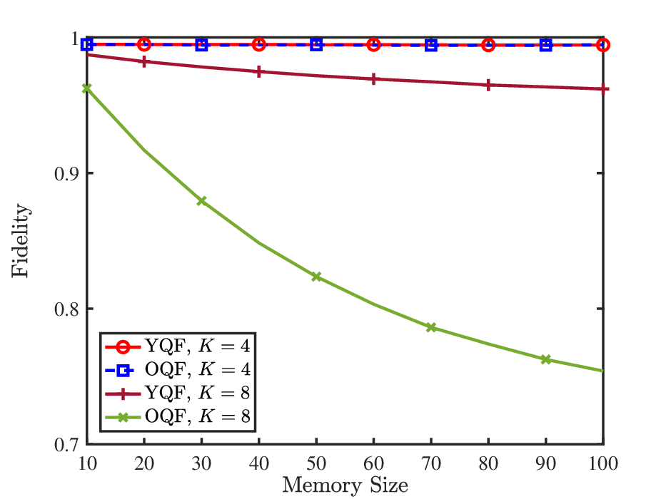
Refer to caption
Fig. 2: Average fidelity as a function of the memory size. The x-axis denote the number of memory slots normalized by KK.
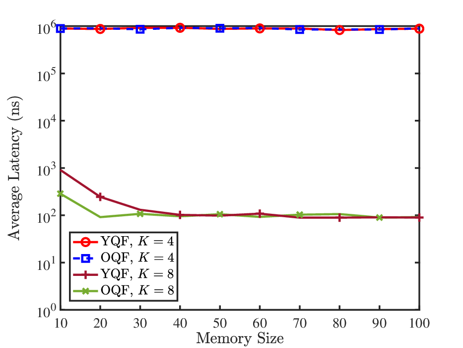
Refer to caption
Fig. 3: Average latency as a function of the memory size. The x-axis denote the number of memory slots normalized by KK.

Figures 2 and 3 respectively show average fidelity and latency of the quantum switch achieved by the on-demand protocols (yqf and oqf) as functions of the number of memory slots. In these two figures, we set ∑i,jλi​j=1.2/μ​s\sum_{i,j}\lambda_{ij}=1.2/\mu\mathrm{s}. First, for K=8K=8, the average fidelity and average latency decrease with memory size; for K=4K=4, the average fidelity and average latency remain constant. This is because for K=4K=4, the rates (λi​j)1≤i,j≤4(\lambda_{ij})_{1\leq i,j\leq 4} lie outside the capacity region. Therefore, the quantum switch is not stable, leading to high latencies. Since there are many unaddressed entanglement requests most of the time, the generated qubits between the switch and end nodes are used immediately for entanglement swapping, and this leads to a fidelity close to one. An increase in memory slots results in qubits staying in the memory longer before consumed, leading to a decrease in fidelity. In addition, more memory slots imply that the quantum switch discards fewer epr pairs and therefore reduces latency. Second, the latency reduction due to the increase in memory size becomes less significant when the number of the memory slots goes beyond 30. This is because, when the number of the memory slots is sufficiently large, the quantum switch can accommodate enough epr pairs to address the entanglement requests, and more memory slots provide diminishing marginal benefit.

Refer to caption
Fig. 4: Average fidelity as a function of T2T_{2}.
Refer to caption
Fig. 5: Average latency as a function of T2T_{2}.

Figures 4 and 5 respectively show average fidelity and latency of the quantum switch achieved by the on-demand protocols (yqf and oqf) as functions of decoherence time T2T_{2}. In these two figures, we set ∑i,jλi​j=1.2/μ​s\sum_{i,j}\lambda_{ij}=1.2/\mu\mathrm{s}. First, fidelity increases with T2T_{2}. This is consistent with the dephasing noise model shown earlier, where we can find that the dephasing probability decreases with T2T_{2}. Second, latency remains constant as a function of T2T_{2}. In the considered setup, T2T_{2} has little effect on the amount or the timing of entanglement generation, and thus the latencies of entanglement requests hardly depend on T2T_{2}. Third, similarly to Figures 2 and 3, yqf and oqf have almost the same performance when K=4K=4. Again this is because the quantum switch is not stable for K=4K=4, and thus the generated qubits between the switch and end nodes are used immediately so that the yqf and oqf give the same choice of epr pairs.

Refer to caption
Fig. 6: Average fidelity as a function of entanglement swapping success probability qq.
Refer to caption
Fig. 7: Average latency as a function of entanglement swapping success probability qq.

Figures 6 and 7 respectively show average fidelity and latency of the quantum switch achieved by the on-demand protocols (yqf and oqf) as functions of the entanglement swapping success probability qq. In these two figures, we set ∑i,jλi​j=2/μ​s\sum_{i,j}\lambda_{ij}=2/\mu\mathrm{s}. First, fidelity initially decreases with qq and then remains constant. This is because for small qq, the rates are outside the capacity region, and the generated qubits between the switch and end nodes are used immediately for entanglement swapping, leading to fidelities close to one. As qq increases, the rates gradually move into the capacity region, and some qubits stay in the memory before being consumed for entanglement swapping, leading to a decrease in fidelity. When qq is sufficiently large, the memory slots are full most of the time, and increasing qq does not significantly improve the memory occupancy rate. In these occasions, average fidelity does not change with qq. Second, average latency first deceases with qq and then remains constant. The reasoning for this behavior is almost the same as that for fidelity. Third, one observes that the sudden change of fidelity and latency occurs around q=0.33q=0.33 for K=8K=8 and q=0.67q=0.67 for K=4K=4. These two points exactly correspond to the boundary points for the capacity region. This shows that the switch demonstrate entirely different behavior inside or outside the capacity region, which is consistent with the stability analysis in earlier sections. This figure also shows that if qq corresponds to a boundary point of the capacity region, increasing qq provides limited performance improvement.

IX Conclusion

We develop efficient entanglement swapping protocols for a quantum switch and analyze their performance in terms of stability of the switch, fidelity of epr pairs and latency of entanglement requests. We determine the capacity region for entanglement rates under the assumption of infinite memory size and infinite qubit lifetime. Specifically, we show that no entanglement swapping protocols can stabilize the switch if the entanglement rates lie outside this capacity region, and develop different protocols that stabilize the switch when the entanglement rates correspond to an interior point of the capacity region. The performance of the developed protocols is evaluated using NetSquid, and practical constraints such as decoherence in memory slots are accounted for. We show that stationary protocols and on-demand protocols exhibit high fidelity and low latency. Moreover, the tradeoff between memory size, decoherence rate, fidelity, and latency shown in the simulation results offer guidance in the implementation of quantum switches.

A potential future direction is the design and analysis of switches with a finite memory size and finite lifetime. Note that in this manuscript, simulation results are obtained in practical scenarios, whereas the stability analysis is based on the assumptions that the switch has sufficiently many memory slots and that qubits have infinite lifetime when stored in the memory. The capacity region for a finite memory size and lifetime must be different, and the entanglement swapping protocols must be designed accordingly.

Acknowledgment

The authors wish to thank Philippe Nain for his helpful suggestions and careful reading of the manuscript.

References

  • [1] P. W. Shor and J. Preskill, “Simple proof of security of the bb84 quantum key distribution protocol,” Phys. Rev. Lett., vol. 85, no. 2, p. 441, 2000.
  • [2] H.-K. Lo and H. F. Chau, “Unconditional security of quantum key distribution over arbitrarily long distances,” Science, vol. 283, no. 5410, pp. 2050–2056, 1999.
  • [3] D. Gottesman, H.-K. Lo, N. Lütkenhaus, and J. Preskill, “Security of quantum key distribution with imperfect devices,” in Proc. IEEE Int. Symp. on Inf. Theory, Chicago, USA, 2006, p. 135.
  • [4] C. H. Bennett, G. Brassard, C. Crépeau, R. Jozsa, A. Peres, and W. K. Wootters, “Teleporting an unknown quantum state via dual classical and Einstein-Podolsky-Rosen channels,” Phys. Rev. Lett., vol. 70, no. 13, pp. 1895–1899, Mar. 1993.
  • [5] X.-S. Ma, T. Herbst, T. Scheidl, D. Wang, S. Kropatschek, W. Naylor, B. Wittmann, A. Mech, J. Kofler, E. Anisimova et al., “Quantum teleportation over 143 kilometres using active feed-forward,” Nature, vol. 489, no. 7415, p. 269, 2012.
  • [6] W. Pfaff, B. J. Hensen, H. Bernien, S. B. van Dam, M. S. Blok, T. H. Taminiau, M. J. Tiggelman, R. N. Schouten, M. Markham, D. J. Twitchen, and R. Hanson, “Unconditional quantum teleportation between distant solid-state quantum bits,” Science, vol. 345, no. 6196, pp. 532–535, Aug. 2014.
  • [7] G. M. D’Ariano, P. L. Presti, and M. G. A. Paris, “Using entanglement improves the precision of quantum measurements,” Phys. Rev. Lett., vol. 87, no. 27, p. 270404, Dec. 2001.
  • [8] Z. Huang, C. Macchiavello, and L. Maccone, “Usefulness of entanglement-assisted quantum metrology,” Phys. Rev. A, vol. 94, no. 1, p. 012101, Jul. 2016.
  • [9] R. Demkowicz-Dobrzański and L. Maccone, “Using entanglement against noise in quantum metrology,” Phys. Rev. Lett., vol. 113, no. 25, p. 250801, Dec. 2014.
  • [10] L. Tassiulas and A. Ephremides, “Stability properties of constrained queueing systems and scheduling policies for maximum throughput in multihop radio networks,” IEEE Trans. Autom. Control, vol. 37, no. 12, pp. 1936–1948, Dec. 1992.
  • [11] M. J. Neely, E. Modiano, and C. E. Rohrs, “Dynamic power allocation and routing for time-varying wireless networks,” IEEE J. Sel. Areas Commun., vol. 23, no. 1, pp. 89–103, Jan. 2005.
  • [12] L. Tassiulas and A. Ephremides, “Dynamic server allocation to parallel queues with randomly varying connectivity,” IEEE Trans. Inf. Theory, vol. 39, no. 2, pp. 466–478, Mar. 1993.
  • [13] M. Żukowski, A. Zeilinger, M. A. Horne, and A. K. Ekert, “‘Event-ready-detectors’ Bell experiment via entanglement swapping,” Phys. Rev. Lett., vol. 71, no. 26, pp. 4287–4290, December 1993.
  • [14] F. Ewert and P. van Loock, “3/4-efficient bell measurement with passive linear optics and unentangled ancillae,” Phys. Rev. Lett., vol. 113, no. 14, p. 140403, Oct. 2014.
  • [15] W. P. Grice, “Arbitrarily complete bell-state measurement using only linear optical elements,” Phys. Rev. A, vol. 84, no. 4, p. 042331, 2011.
  • [16] P. Kok, W. J. Munro, K. Nemoto, T. C. Ralph, J. P. Dowling, and G. J. Milburn, “Linear optical quantum computing with photonic qubits,” Rev. Mod. Phys., vol. 79, no. 1, pp. 135–174, 2007.
  • [17] L.-M. Duan and H. J. Kimble, “Scalable photonic quantum computation through cavity-assisted interactions,” Phys. Rev. Lett., vol. 9, no. 12, p. 127902, Mar. 2004.
  • [18] P. Nain, G. Vardoyan, S. Guha, and D. Towsley, “On the analysis of a multipartite entanglement distribution switch,” Proc. ACM Meas. Anal. Comput. Syst., vol. 4, no. 2, Jun. 2020.
  • [19] G. Vardoyan, S. Guha, P. Nain, and D. Towsley, “On the stochastic analysis of a quantum entanglement distribution switch,” IEEE Trans. Quantum Engineering, vol. 2, p. 4101016, Feb. 2021.
  • [20] ——, “On the exact analysis of an idealized quantum switch,” Perform. Eval., vol. 144, no. 102141, Dec. 2020.
  • [21] ——, “On the capacity region of bipartite and tripartite entanglement switching,” ACM SIGMETRICS Performance Evaluation Review, vol. 48, no. 3, pp. 45–50, Dec. 2020.
  • [22] T. Vasantam and D. Towsley, “Stability analysis of a quantum network with max-weight scheduling,” arXiv, 2021. [Online]. Available: https://arxiv.org/abs/2106.00831
  • [23] E. Shchukin, F. Schmidt, and P. van Loock, “Waiting time in quantum repeaters with probabilistic entanglement swapping,” Phys. Rev. A, vol. 100, no. 3, p. 032322, 2019.
  • [24] P. Walters, An Introduction to Ergodic Theory, 1st ed. New York: Springer-Verlag, 1982.
  • [25] T. Coopmans et al., “NetSquid, a discrete-event simulation platform for quantum networks,” Commun Phys, vol. 4, no. 164, 2021.
  • [26] M. Bhaskar, R. Riedinger, B. Machielse et al., “Experimental demonstration of memory-enhanced quantum communication,” Nature, vol. 580, pp. 60–64, 2020.
  • [27] J. Preskill, “Lecture notes for Physics 219,” 2015.
  • [28] M. J. Neely, “Dynamic Power Allocation and Routing for Satellite and Wireless Networks with Time Varying Channels,” Ph.D. dissertation, Department of Electrical Engineering and Computer Science, Massachusetts Institute of Technology, Cambridge, MA, Nov. 2003, thesis advisor: Professor Eytan Modiano.

Appendix A Proof of Theorem 1

Here we prove that (λi​j)∈𝚲(\lambda_{ij})\in\bm{\Lambda} is necessary for the quantum switch to be stable. The following lemma is inspired by Lemma 1 in [28].

Lemma 5

If a quantum switch is stable, then for any δ>0\delta>0, there exits a finite value VV such that for any t0>0t_{0}>0, there exists t~>t0\tilde{t}>t_{0} such that

ℙ[Ui​j(t~)≤V]>1−δ,∀i,j∈𝒦.\displaystyle\mathbb{P}\big[U_{ij}(\tilde{t})\leq V\big]>1-\delta,\quad\forall i,j\in\mathcal{K}. (53)

In particular, for the case δ=1/2\delta=1/2, there exists a value VV such that the probability that the unfinished requests in all queues, i.e., Ui​j​(t)U_{ij}(t), i,j∈𝒦i,j\in\mathcal{K}, simultaneously drop below VV is greater than 1/21/2 infinitely often.

Consider a quantum switch with request rate matrix (λi​j)i,j∈𝒦(\lambda_{ij})_{i,j\in\mathcal{K}}. Suppose there exists an entanglement swapping algorithm that stabilizes the quantum switch. We need to show that there exist variables {fi​j}i,j∈𝒦\{f_{ij}\}_{i,j\in\mathcal{K}} satisfying (8)-(10). With the notations defined in Section IV-A, we have for arbitrary time slot t≥0t\geq 0,

∑τ=0t−1∑i∈𝒦Fi​j​(τ)\displaystyle\sum_{\tau=0}^{t-1}\sum_{i\in\mathcal{K}}F_{ij}(\tau) ≤∑τ=0t−1C0​j​(τ),∀j∈𝒦\displaystyle\leq\sum_{\tau=0}^{t-1}C_{0j}(\tau),\quad\forall j\in\mathcal{K} (54)
∑i,j∈𝒦Fi​j​(t)\displaystyle\sum_{i,j\in\mathcal{K}}F_{ij}(t) ≤W\displaystyle\leq W (55)
Ui​j​(t)\displaystyle U_{ij}(t) =max⁡{∑τ=0t−1Ai​j​(τ)−∑τ=0t−1μi​j​(τ),0},∀i,j∈𝒦.\displaystyle=\max\bigg\{\sum_{\tau=0}^{t-1}A_{ij}(\tau)-\sum_{\tau=0}^{t-1}\mu_{ij}(\tau),0\bigg\},\quad\forall i,j\in\mathcal{K}. (56)

Fix arbitrarily small ϵ>0\epsilon>0, and set δ=1/2\delta=1/2. According to Lemma 5, there exists finite VV and t~\tilde{t} such that t~≥V/ϵ\tilde{t}\geq V/\epsilon and

ℙ[Ui​j(t~)≤V]>1/2.\displaystyle\mathbb{P}\big[U_{ij}(\tilde{t})\leq V\big]>1/2. (57)

Hence,

ℙ[Ui​j(t~)/t~≤ϵ]\displaystyle\mathbb{P}\big[{U_{ij}(\tilde{t})}/{\tilde{t}}\leq\epsilon\big] =ℙ[Ui​j(t~)≤t~ϵ]≥ℙ[Ui​j(t~)≤V]≥1/2.\displaystyle=\mathbb{P}\big[U_{ij}(\tilde{t})\leq\tilde{t}\epsilon\big]\geq\mathbb{P}\big[U_{ij}(\tilde{t})\leq V\big]\geq 1/2.

We then define the following event A0A_{0}: Ui​j​(t~)/t~≤ϵ,∀i,j∈𝒦{U_{ij}(\tilde{t})}/{\tilde{t}}\leq\epsilon,\quad\forall i,j\in\mathcal{K}. It follows that ℙ⁡[A0]≥1/2\mathbb{P}[A_{0}]\geq 1/2.

We now consider the following events:

A1:1t~​∑τ=0t~−1Ai​j​(τ)≥λi​j−ϵ,∀i,j∈𝒦\displaystyle A_{1}:~\frac{1}{\tilde{t}}\sum_{\tau=0}^{\tilde{t}-1}A_{ij}(\tau)\geq\lambda_{ij}-\epsilon,\quad\forall i,j\in\mathcal{K} (58)
A2:1t~​∑τ=0t~−1C0​i​(τ)≤pi+ϵ,∀i∈𝒦\displaystyle A_{2}:~\frac{1}{\tilde{t}}\sum_{\tau=0}^{\tilde{t}-1}C_{0i}(\tau)\leq p_{i}+\epsilon,\quad\forall i\in\mathcal{K} (59)
A3:∑τ=0t~−1μi​j​(τ)∑τ=0t~−1Fi​j​(τ)≤q+ϵ,∀i,j∈𝒦.\displaystyle A_{3}:~\frac{\sum_{\tau=0}^{\tilde{t}-1}\mu_{ij}(\tau)}{\sum_{\tau=0}^{\tilde{t}-1}F_{ij}(\tau)}\leq q+\epsilon,\quad\forall i,j\in\mathcal{K}. (60)

Since [∑t=0t−1Ai​j​(t)]/t[\sum_{t=0}^{t-1}A_{ij}(t)]/t converges to λi​j\lambda_{ij} almost surely due to Birkhoff-Khinchin theorem, it converges to λi​j\lambda_{ij} in probability. This means that ℙ⁡[A1]≥0.99\mathbb{P}[A_{1}]\geq 0.99 for sufficiently large t~\tilde{t}. Similarly, since {C0​i​(t):t≥0}\{{C}_{0i}(t):t\geq 0\} are i.i.d with respect to tt, ℙ⁡[A2]≥0.99\mathbb{P}[A_{2}]\geq 0.99 for sufficiently large t~\tilde{t}. Regarding the event A3A_{3}, since entanglement swapping succeeds with probability qq, the probability of A3A_{3} is no less than 0.99 for sufficiently large ∑τ=0t~−1Fi​j​(τ)\sum_{\tau=0}^{\tilde{t}-1}F_{ij}(\tau). Note that when events A0A_{0} and A1A_{1} occur simultaneously, ∀i,j∈𝒦\forall i,j\in\mathcal{K}

∑τ=0t~−1Fi​j​(τ)\displaystyle\sum_{\tau=0}^{\tilde{t}-1}F_{ij}(\tau) ≥∑τ=0t~−1μi​j​(τ)≥[∑τ=0t~−1Ai​j​(τ)]−Ui​j​(t~)≥(λi​j−ϵ)​t~−V\displaystyle\geq\sum_{\tau=0}^{\tilde{t}-1}\mu_{ij}(\tau)\geq\bigg[\sum_{\tau=0}^{\tilde{t}-1}A_{ij}(\tau)\bigg]-U_{ij}(\tilde{t})\geq(\lambda_{ij}-\epsilon)\tilde{t}-V

where the second inequality comes from (56), and the last inequality follows from the joint occurrence of the events A0A_{0} and A1A_{1}. Hence, ∑τ=0t~−1Fi​j​(τ)\sum_{\tau=0}^{\tilde{t}-1}F_{ij}(\tau) can be made arbitrarily large through choice of t~\tilde{t}. Consider the joint event ∩l=03Al\cap_{l=0}^{3}A_{l}; its probability can be lower bounded as follows:

ℙ[∩l=03Al]\displaystyle\mathbb{P}\big[\cap_{l=0}^{3}A_{l}\big] =1−ℙ[∪l=03A¯l]≥12−ℙ[∪l=13A¯l]≥12−ℙ[A¯1]−ℙ[A¯2]−ℙ[A1∩A2∩A¯3]\displaystyle=1-\mathbb{P}\big[\cup_{l=0}^{3}\overline{A}_{l}\big]\geq\frac{1}{2}-\mathbb{P}\big[\cup_{l=1}^{3}\overline{A}_{l}\big]\geq\frac{1}{2}-\mathbb{P}\big[\overline{A}_{1}\big]-\mathbb{P}\big[\overline{A}_{2}\big]-\mathbb{P}\big[{A}_{1}\cap{A}_{2}\cap\overline{A}_{3}\big]
≥12−0.01−0.01−0.01>0.\displaystyle\geq\frac{1}{2}-0.01-0.01-0.01>0. (61)

Now define

fi​j​(t~)=1t~​∑τ=0t~−1Fi​j​(τ)∀i,j∈𝒦\displaystyle f_{ij}(\tilde{t})=\frac{1}{\tilde{t}}\sum_{\tau=0}^{\tilde{t}-1}F_{ij}(\tau)\quad\forall i,j\in\mathcal{K}

and the following events:

A4:∑i∈𝒦fi​j​(t~)≤pj+ϵ,∀j∈𝒦\displaystyle A_{4}:~\sum_{i\in\mathcal{K}}f_{ij}(\tilde{t})\leq p_{j}+\epsilon,\quad\forall j\in\mathcal{K} (62)
A5:∑i,j∈𝒦fi​j​(t~)≤W\displaystyle A_{5}:~\sum_{i,j\in\mathcal{K}}f_{ij}(\tilde{t})\leq W (63)
A6:λi​j−ϵ≤ϵ+(q+ϵ)​fi​j​(t~),∀i,j∈𝒦.\displaystyle A_{6}:~\lambda_{ij}-\epsilon\leq\epsilon+(q+\epsilon)f_{ij}(\tilde{t}),\quad\forall i,j\in\mathcal{K}. (64)

We next show that ∩l=03Al⊆A4∩A5∩A6\cap_{l=0}^{3}A_{l}\subseteq A_{4}\cap A_{5}\cap A_{6}. In fact, if ∩l=03Al\cap_{l=0}^{3}A_{l} occurs, we will show that A4∩A5∩A6A_{4}\cap A_{5}\cap A_{6} occurs. For all jj,

∑i∈𝒦fi​j​(t~)=1t~​∑τ=0t~−1∑i∈𝒦Fi​j​(τ)≤1t~​∑τ=0t~−1C0​j​(τ)≤pj+ϵ\displaystyle\sum_{i\in\mathcal{K}}f_{ij}(\tilde{t})=\frac{1}{\tilde{t}}\sum_{\tau=0}^{\tilde{t}-1}\sum_{i\in\mathcal{K}}F_{ij}(\tau)\leq\frac{1}{\tilde{t}}\sum_{\tau=0}^{\tilde{t}-1}C_{0j}(\tau)\leq p_{j}+\epsilon

where the first inequality is because of (54) and the second inequality is because A2A_{2} occurs. Hence, event A4A_{4} occurs. Moreover,

∑i,j∈𝒦fi​j​(t~)=1t~​∑τ=0t~−1∑i∈𝒦Fi​j​(τ)≤W\displaystyle\sum_{i,j\in\mathcal{K}}f_{ij}(\tilde{t})=\frac{1}{\tilde{t}}\sum_{\tau=0}^{\tilde{t}-1}\sum_{i\in\mathcal{K}}F_{ij}(\tau)\leq W

where the inequality comes from (55). Hence, event A5A_{5} occurs. In addition, for all i,j∈𝒦i,j\in\mathcal{K}

λi​j−ϵ\displaystyle\lambda_{ij}-\epsilon ≤1t~​∑τ=0t~−1Ai​j​(τ)≤1t~​[Ui​j​(t~)+∑τ=0t~−1μi​j​(τ)]≤ϵ+q+ϵt~​∑τ=0t~−1Fi​j​(τ)≤ϵ+(q+ϵ)​fi​j​(t~)\displaystyle\leq\frac{1}{\tilde{t}}\sum_{\tau=0}^{\tilde{t}-1}A_{ij}(\tau)\leq\frac{1}{\tilde{t}}\bigg[U_{ij}(\tilde{t})+\sum_{\tau=0}^{\tilde{t}-1}\mu_{ij}(\tau)\bigg]\leq\epsilon+\frac{q+\epsilon}{\tilde{t}}\sum_{\tau=0}^{\tilde{t}-1}F_{ij}(\tau)\leq\epsilon+(q+\epsilon)f_{ij}(\tilde{t})

where the first inequality is because A1A_{1} occurs, the second inequality comes from (56), and the third inequality is because A0A_{0} and A3A_{3} occur. Hence, the event A6A_{6} occurs. This shows that ∩l=03Al⊆A4∩A5∩A6\cap_{l=0}^{3}A_{l}\subseteq A_{4}\cap A_{5}\cap A_{6}. Therefore, ℙ[A4∩A5∩A6]≥ℙ[∩l=03Al]>0\mathbb{P}[A_{4}\cap A_{5}\cap A_{6}]\geq\mathbb{P}\big[\cap_{l=0}^{3}A_{l}\big]>0, where the last inequality is because of (61). Then, with nonzero probability, the variables {fi​j​(t~)}i,j∈𝒦\{f_{ij}(\tilde{t})\}_{i,j\in\mathcal{K}} defined based on Fi​j​(τ)F_{ij}(\tau) satisfy (62)-(64). It follows that for arbitrarily small ϵ>0\epsilon>0, there exist {fi​j}i,j∈𝒦\{f_{ij}\}_{i,j\in\mathcal{K}} that satisfy

∑i∈𝒦fi​j≤pj+ϵ,∀j∈𝒦\displaystyle\sum_{i\in\mathcal{K}}f_{ij}\leq p_{j}+\epsilon,\quad\forall j\in\mathcal{K}
∑i,j∈𝒦fi​j≤W\displaystyle\sum_{i,j\in\mathcal{K}}f_{ij}\leq W
λi​j−ϵ≤ϵ+(q+ϵ)​fi​j,∀i,j∈𝒦.\displaystyle\lambda_{ij}-\epsilon\leq\epsilon+(q+\epsilon)f_{ij},\quad\forall i,j\in\mathcal{K}.

This proves that (λi​j)i,j∈𝒦(\lambda_{ij})_{i,j\in\mathcal{K}} is a limit point in the capacity region 𝚲\bm{\Lambda} defined in (8)-(10). Since 𝚲\bm{\Lambda} is compact, it follows that (λi​j)i,j∈𝒦∈𝚲(\lambda_{ij})_{i,j\in\mathcal{K}}\in\bm{\Lambda}.

Appendix B Proof of Lemma 1

Without loss of generality, we assume J=0J=0. Consider (22) at times t=m​Tt=mT. Taking expectations of (22) over the distribution of 𝑼⁡(m​T)\bm{U}(mT) and summing over mm from m=0m=0 to M−1M-1 give

𝔼⁡[L⁡(𝑼⁡(M​T))]−𝔼⁡[L⁡(𝑼⁡(0))]≤C​M−∑m=0M−1∑i,j∈𝒦θi​j​𝔼​[Ui​j​(m​T)]\displaystyle\mathbb{E}[L(\bm{U}(MT))]-\mathbb{E}[L(\bm{U}(0))]\leq CM-\sum_{m=0}^{M-1}\sum_{i,j\in\mathcal{K}}\theta_{ij}\mathbb{E}[{U}_{ij}(mT)]

which implies that

1M​∑m=0M−1∑i,j∈𝒦θi​j​𝔼​[Ui​j​(m​T)]≤C+𝔼⁡[L⁡(𝑼⁡(0))]/M.\displaystyle\frac{1}{M}\sum_{m=0}^{M-1}\sum_{i,j\in\mathcal{K}}\theta_{ij}\mathbb{E}[{U}_{ij}(mT)]\leq C+\mathbb{E}[L(\bm{U}(0))]/M.

Then for any i,j∈𝒦i,j\in\mathcal{K},

1M​∑m=0M−1𝔼⁡[Ui​j​(m​T)]≤C+𝔼⁡[L⁡(𝑼⁡(0))]/Mθi​j.\displaystyle\frac{1}{M}\sum_{m=0}^{M-1}\mathbb{E}[{U}_{ij}(mT)]\leq\frac{C+\mathbb{E}[L(\bm{U}(0))]/M}{\theta_{ij}}. (65)

Moreover, for any t0t_{0}, we write t0t_{0} as t0=⌊t0/T⌋​T+τt_{0}=\lfloor t_{0}/T\rfloor T+\tau, where τ\tau is the remainder after diving t0t_{0} by TT, and evidently τ∈{1,2,…,T−1}\tau\in\{1,2,\dotsc,T-1\}. Then for V>T​AmaxV>TA_{\mathrm{max}}

ℙ[Ui​j(t0)>(T+1)V+TAmax]\displaystyle\mathbb{P}[{U}_{ij}(t_{0})>(T+1)V+TA_{\mathrm{max}}] ≤ℙ[Ui​j(⌊t0/T⌋T)>V\displaystyle\leq\mathbb{P}[{U}_{ij}(\lfloor t_{0}/T\rfloor T)>V
or ∃τ0∈{1,2,…,T−1},Ai​j(⌊t0/T⌋T+τ0)>V+Amax]\displaystyle\hskip-42.67912pt\text{ or }\exists\,\tau_{0}\in\{1,2,\dotsc,T-1\},{A}_{ij}(\lfloor t_{0}/T\rfloor T+\tau_{0})>V+A_{\mathrm{max}}] (66)
≤ℙ[Ui​j(⌊t0/T⌋T)>V]+T​Amax2V2.\displaystyle\leq\mathbb{P}[{U}_{ij}(\lfloor t_{0}/T\rfloor T)>V]+\frac{TA^{2}_{\mathrm{max}}}{V^{2}}. (67)

The inequality (66) is because if U⁡(⌊t0/T⌋​T)≤VU(\lfloor t_{0}/T\rfloor T)\leq V and Ai​j​(⌊t0/T⌋​T+τ1)≤V+Amax{A}_{ij}(\lfloor t_{0}/T\rfloor T+\tau_{1})\leq V+A_{\mathrm{max}} holds for τ1=1,2,…,T−1\tau_{1}=1,2,\dotsc,T-1, then

Ui​j​(t0)≤Ui​j​(⌊t0/T⌋​T)+∑τ1=1τAi​j​(⌊t0/T⌋​T+τ1)≤(T+1)​V+T​Amax.\displaystyle{U}_{ij}(t_{0})\leq{U}_{ij}(\lfloor t_{0}/T\rfloor T)+\sum_{\tau_{1}=1}^{\tau}{A}_{ij}(\lfloor t_{0}/T\rfloor T+\tau_{1})\leq(T+1)V+TA_{\mathrm{max}}.

The inequality (67) is due to the union bound and (6). We then have

1t∑τ=0t−1ℙ[Ui​j(τ)>(T+1)V+TAmax]\displaystyle\frac{1}{t}\sum_{\tau=0}^{t-1}\mathbb{P}\big[{U}_{ij}(\tau)>(T+1)V+TA_{\mathrm{max}}\big]
≤1⌊t/T⌋∑m0=0⌊t/T⌋−1ℙ[Ui​j(m0T)>(T+1)V+TAmax]+T​Amax2V2\displaystyle\quad\leq\frac{1}{\lfloor t/T\rfloor}\sum_{m_{0}=0}^{\lfloor t/T\rfloor-1}\mathbb{P}\big[{U}_{ij}(m_{0}T)>(T+1)V+TA_{\mathrm{max}}\big]+\frac{TA^{2}_{\mathrm{max}}}{V^{2}}
≤1⌊t/T⌋​∑m0=0⌊t/T⌋−1𝔼⁡[Ui​j​(m0​T)](T+1)​V+T​Amax+T​Amax2V2\displaystyle\quad\leq\frac{1}{\lfloor t/T\rfloor}\frac{\sum_{m_{0}=0}^{\lfloor t/T\rfloor-1}\mathbb{E}\big[{U}_{ij}(m_{0}T)\big]}{(T+1)V+TA_{\mathrm{max}}}+\frac{TA^{2}_{\mathrm{max}}}{V^{2}}
≤1⌊t/T⌋​θi​j​⌊t/T⌋​C+𝔼⁡[L⁡(𝑼⁡(0))](T+1)​V+T​Amax+T​Amax2V2.\displaystyle\quad\leq\frac{1}{\lfloor t/T\rfloor\theta_{ij}}\frac{\lfloor t/T\rfloor C+\mathbb{E}[L(\bm{U}(0))]}{(T+1)V+TA_{\mathrm{max}}}+\frac{TA^{2}_{\mathrm{max}}}{V^{2}}.

Taking lim supt→∞\limsup_{t\rightarrow\infty}, we see that gi​j​(V)g_{ij}(V) defined in (7) is on the order of O⁡(1/V)O(1/V). Taking limits as V→∞V\rightarrow\infty, we have gi​j​(V)→0g_{ij}(V)\rightarrow 0, i,j∈𝒦i,j\in\mathcal{K}.

Appendix C Proof of Lemma 2

The TT-step dynamics of unprocessed entanglement request satisfies

Ui​j​(t0+T)\displaystyle U_{ij}(t_{0}+T) ≤max⁡{Ui​j​(t0)−Ei​j​(t0)−∑t=t0t0+T−1μi​j​(t),0}+∑t=t0t0+T−1Ai​j​(t)\displaystyle\leq\max\Big\{U_{ij}(t_{0})-E_{ij}(t_{0})-\sum_{t=t_{0}}^{t_{0}+T-1}\mu_{ij}(t),0\Big\}+\sum_{t=t_{0}}^{t_{0}+T-1}A_{ij}(t)
≤max⁡{Ui​j​(t0)−∑t=t0t0+T−1μi​j​(t),0}+∑t=t0t0+T−1Ai​j​(t)\displaystyle\leq\max\Big\{U_{ij}(t_{0})-\sum_{t=t_{0}}^{t_{0}+T-1}\mu_{ij}(t),0\Big\}+\sum_{t=t_{0}}^{t_{0}+T-1}A_{ij}(t)

where the first inequality is because some entanglement requests during the TT-slot interval may be processed and the second inequality is because Ei​j​(t0)≥0E_{ij}(t_{0})\geq 0. Squaring both sides and using the fact that (max⁡{x,0})2≤x2(\max\{x,0\})^{2}\leq x^{2} give

[Ui​j​(t0+T)]2−[Ui​j​(t0)]2\displaystyle\big[U_{ij}(t_{0}+T)\big]^{2}-\big[U_{ij}(t_{0})\big]^{2}
≤[∑t=t0t0+T−1μi​j​(t)]2−2​Ui​j​(t0)​∑t=t0t0+T−1μi​j​(t)+[∑t=t0t0+T−1Ai​j​(t)]2\displaystyle\leq\Big[\sum_{t=t_{0}}^{t_{0}+T-1}\mu_{ij}(t)\Big]^{2}-2U_{ij}(t_{0})\sum_{t=t_{0}}^{t_{0}+T-1}\mu_{ij}(t)+\Big[\sum_{t=t_{0}}^{t_{0}+T-1}A_{ij}(t)\Big]^{2}
+2max{Ui​j(t0)−∑t=t0t0+T−1μi​j(t),0}∑t=t0t0+T−1Ai​j(t)\displaystyle\quad+2\max\Big\{U_{ij}(t_{0})-\sum_{t=t_{0}}^{t_{0}+T-1}\mu_{ij}(t),0\Big\}\sum_{t=t_{0}}^{t_{0}+T-1}A_{ij}(t)
≤[∑t=t0t0+T−1μi​j​(t)]2+[∑t=t0t0+T−1Ai​j​(t)]2+2​Ui​j​(t0)​∑t=t0t0+T−1[Ai​j​(t)−μi​j​(t)].\displaystyle\leq\Big[\sum_{t=t_{0}}^{t_{0}+T-1}\mu_{ij}(t)\Big]^{2}+\Big[\sum_{t=t_{0}}^{t_{0}+T-1}A_{ij}(t)\Big]^{2}+2U_{ij}(t_{0})\sum_{t=t_{0}}^{t_{0}+T-1}\Big[A_{ij}(t)-\mu_{ij}(t)\Big].

Taking conditional expectations on both sides and noting that

𝔼⁡[(∑t=t0t0+T−1Ai​j​(t))2|𝑼⁡(t0)=𝒖]≤T​∑t=t0t0+T−1𝔼⁡[Ai​j2​(t)|𝑼⁡(t0)=𝒖]≤T2​Amax2\displaystyle\mathbb{E}\bigg[\Big(\sum_{t=t_{0}}^{t_{0}+T-1}{A}_{ij}(t)\Big)^{2}\big|\bm{U}(t_{0})=\bm{u}\bigg]\leq T\sum_{t=t_{0}}^{t_{0}+T-1}\mathbb{E}\bigg[{A}^{2}_{ij}(t)\big|\bm{U}(t_{0})=\bm{u}\bigg]\leq T^{2}A^{2}_{\mathrm{max}}

we have the desired result.

Appendix D Proof of Lemma 3

Since 𝚲\bm{\Lambda} is an interior point of the capacity region, there exists δ>0\delta>0 such that ∑i∈𝒦λi​j<q⁡(1−δ)​pj\sum_{i\in\mathcal{K}}\lambda_{ij}<q(1-\delta)p_{j}, ∀j\forall j. Set ϵ\epsilon to be a positive number such that

maxj∈𝒦⁡2​ϵpj+ϵ+q⁡(1−δ)​(1+δmax)​pjpj+ϵ≤q⁡(1−δ/2)\displaystyle\max_{j\in\mathcal{K}}\frac{2\epsilon}{p_{j}+\epsilon}+q(1-\delta)(1+\delta_{\mathrm{max}})\frac{p_{j}}{p_{j}+\epsilon}\leq q(1-\delta/2) (68)

where δmax=maxi,j⁡ϵ/λi​j\delta_{\mathrm{max}}=\max_{i,j}{\epsilon}/{\lambda_{ij}}. Such an ϵ\epsilon must exist because of the mean value theorem.66 6 Note that the left-hand side is q⁡(1−δ)q(1-\delta) and ∞\infty when ϵ\epsilon takes the value 00 and ∞\infty, respectively. We then define the following events:

B1:∃i,j,|1t+1​∑τ=0tAi​j​(τ)−λi​j|>ϵ\displaystyle B_{1}:\exists i,j,~\bigg|\frac{1}{t+1}\sum_{\tau=0}^{t}A_{ij}(\tau)-\lambda_{ij}\bigg|>\epsilon
B2:∃j,|1t+1​∑τ=0tC0​j​(τ)−pj|>ϵ\displaystyle B_{2}:\exists j,~\bigg|\frac{1}{t+1}\sum_{\tau=0}^{t}C_{0j}(\tau)-p_{j}\bigg|>\epsilon
B3:∃i,j,∑τ=0t−1μi​j​(τ)∑τ=0t−1Fi​j​(τ)≤q⁡(1−δ2/4)​ and ​∑τ=0t−1Fi​j​(τ)≥δ​t​[(pj−ϵ)−q⁡(1−δ)​pj​(1+δmax)]K⁡(2+δ)>0.\displaystyle B_{3}:\exists i,j,~\frac{\sum_{\tau=0}^{t-1}\mu_{ij}(\tau)}{\sum_{\tau=0}^{t-1}F_{ij}(\tau)}\leq q(1-\delta^{2}/4)\text{ and }\sum_{\tau=0}^{t-1}F_{ij}(\tau)\geq\frac{\delta t[(p_{j}-\epsilon)-q(1-\delta)p_{j}(1+\delta_{\mathrm{max}})]}{K(2+\delta)}>0.

We next bound the set S¯​(t)\overline{S}(t).

Lemma 6

The following relationship holds:

S¯​(t)⊆B1∪B2∪B3.\displaystyle\overline{S}(t)\subseteq B_{1}\cup B_{2}\cup B_{3}. (69)
Proof:

To show (69) holds, we only need to show that S¯​(t)∩B¯1∩B¯2⊆B3\overline{S}(t)\cap\overline{B}_{1}\cap\overline{B}_{2}\subseteq B_{3}.

In fact, if S¯​(t)∩B¯1∩B¯2\overline{S}(t)\cap\overline{B}_{1}\cap\overline{B}_{2} occurs, then the definition of S⁡(t)S(t) implies that ∃j0\exists j_{0} such that

∑i∈𝒦[Ui​j0​(t)+Ai​j​(t)]>E0​j0​(t)+C0​j0​(t).\displaystyle\sum_{i\in\mathcal{K}}[U_{ij_{0}}(t)+A_{ij}(t)]>E_{0j_{0}}(t)+C_{0j_{0}}(t). (70)

The requirement (15) in on-demand protocols implies that

Ui​j0​(t)=∑τ=0t−1Ai​j0​(τ)−∑τ=0t−1μi​j0​(τ).\displaystyle U_{ij_{0}}(t)=\sum_{\tau=0}^{t-1}A_{ij_{0}}(\tau)-\sum_{\tau=0}^{t-1}\mu_{ij_{0}}(\tau).

Together with (70), we have

∑i∈𝒦[∑τ=0tAi​j0​(τ)−∑τ=0t−1μi​j0​(τ)]>∑τ=0tC0​j0​(τ)−∑i∈𝒦∑τ=0t−1Fi​j0​(τ).\displaystyle\sum_{i\in\mathcal{K}}\Big[\sum_{\tau=0}^{t}A_{ij_{0}}(\tau)-\sum_{\tau=0}^{t-1}\mu_{ij_{0}}(\tau)\Big]>\sum_{\tau=0}^{t}C_{0j_{0}}(\tau)-\sum_{i\in\mathcal{K}}\sum_{\tau=0}^{t-1}F_{ij_{0}}(\tau). (71)

Then we have

∑i∈𝒦∑τ=0t−1Fi​j0​(τ)−∑i∈𝒦∑τ=0t−1μi​j0​(τ)\displaystyle\sum_{i\in\mathcal{K}}\sum_{\tau=0}^{t-1}F_{ij_{0}}(\tau)-\sum_{i\in\mathcal{K}}\sum_{\tau=0}^{t-1}\mu_{ij_{0}}(\tau)
>(pj0−ϵ)​(t+1)−∑i∈𝒦(λi​j0+ϵ)​(t+1)\displaystyle>(p_{j_{0}}-\epsilon)(t+1)-\sum_{i\in\mathcal{K}}(\lambda_{ij_{0}}+\epsilon)(t+1)
>(pj0−ϵ)​(t+1)−(1+δmax)​∑i∈𝒦λi​j0​(t+1)\displaystyle>(p_{j_{0}}-\epsilon)(t+1)-(1+\delta_{\mathrm{max}})\sum_{i\in\mathcal{K}}\lambda_{ij_{0}}(t+1)
>(pj0−ϵ)​(t+1)−q⁡(1−δ)​pj0​(1+δmax)​(t+1)\displaystyle>(p_{j_{0}}-\epsilon)(t+1)-q(1-\delta)p_{j_{0}}(1+\delta_{\mathrm{max}})(t+1) (72)
>[pj0−ϵpj0+ϵ−q⁡(1−δ)​(1+δmax)​pj0pj0+ϵ]​∑τ=0tC0​j0​(τ)\displaystyle>\bigg[\frac{p_{j_{0}}-\epsilon}{p_{j_{0}}+\epsilon}-q(1-\delta)(1+\delta_{\mathrm{max}})\frac{p_{j_{0}}}{p_{j_{0}}+\epsilon}\bigg]\sum_{\tau=0}^{t}C_{0j_{0}}(\tau)
≥[pj0−ϵpj0+ϵ−q⁡(1−δ)​(1+δmax)​pj0pj0+ϵ]​∑i∈𝒦∑τ=0t−1Fi​j0​(τ)\displaystyle\geq\bigg[\frac{p_{j_{0}}-\epsilon}{p_{j_{0}}+\epsilon}-q(1-\delta)(1+\delta_{\mathrm{max}})\frac{p_{j_{0}}}{p_{j_{0}}+\epsilon}\bigg]\sum_{i\in\mathcal{K}}\sum_{\tau=0}^{t-1}F_{ij_{0}}(\tau) (73)

where the first inequality is obtained by reordering (71) and using the fact that B¯1∩B¯2\overline{B}_{1}\cap\overline{B}_{2} occurs, the third inequality is because ∑i∈𝒦λi​j0<q⁡(1−δ)​pj0\sum_{i\in\mathcal{K}}\lambda_{ij_{0}}<q(1-\delta)p_{j_{0}}, and the fourth inequality is because B¯2\overline{B}_{2} occurs and

pj0−ϵpj0+ϵ−q⁡(1−δ)​(1+δmax)​pj0pj0+ϵ\displaystyle\frac{p_{j_{0}}-\epsilon}{p_{j_{0}}+\epsilon}-q(1-\delta)(1+\delta_{\mathrm{max}})\frac{p_{j_{0}}}{p_{j_{0}}+\epsilon} =1−[2​ϵpj0+ϵ+q⁡(1−δ)​(1+δmax)​pj0pj0+ϵ]\displaystyle=1-\bigg[\frac{2\epsilon}{p_{j_{0}}+\epsilon}+q(1-\delta)(1+\delta_{\mathrm{max}})\frac{p_{j_{0}}}{p_{j_{0}}+\epsilon}\bigg]
≥1−q⁡(1−δ/2)\displaystyle\geq 1-q(1-\delta/2) (74)
>1−q>0\displaystyle>1-q>0

in which (74) is due to (68). We next show that if (72) and (73) hold, then B3B_{3} occurs, showing that S¯​(t)∩B¯1∩B¯2⊆B3\overline{S}(t)\cap\overline{B}_{1}\cap\overline{B}_{2}\subseteq B_{3} and the proof is finished.

In fact, (68) and (73) and imply

q⁡(1−δ/2)​∑i∈𝒦∑τ=0t−1Fi​j0​(τ)≥∑i∈𝒦∑τ=0t−1μi​j0​(τ).\displaystyle q(1-\delta/2)\sum_{i\in\mathcal{K}}\sum_{\tau=0}^{t-1}F_{ij_{0}}(\tau)\geq\sum_{i\in\mathcal{K}}\sum_{\tau=0}^{t-1}\mu_{ij_{0}}(\tau).

Using the following lemma with

ai\displaystyle a_{i} =∑τ=0t−1Fi​j0​(τ)\displaystyle=\sum_{\tau=0}^{t-1}F_{ij_{0}}(\tau)
bi\displaystyle b_{i} =∑τ=0t−1μi​j0​(τ)\displaystyle=\sum_{\tau=0}^{t-1}\mu_{ij_{0}}(\tau)
c\displaystyle c =q⁡(1−δ/2)\displaystyle=q(1-\delta/2)
d\displaystyle d =(pj0−ϵ)​t−q⁡(1−δ)​pj0​(1+δmax)​t\displaystyle=(p_{j_{0}}-\epsilon)t-q(1-\delta)p_{j_{0}}(1+\delta_{\mathrm{max}})t
δ0\displaystyle\delta_{0} =δ/2\displaystyle=\delta/2

and we have the desired result that B3B_{3} occurs.

Lemma 7

For ai,bi∈ℝ≥0a_{i},b_{i}\in\mathbb{R}_{\geq 0}, i=1,2,…,Ki=1,2,\dots,K and c,d>0c,d>0, if

c​∑i=1Kai\displaystyle c\sum_{i=1}^{K}a_{i} ≥∑i=1Kbi\displaystyle\geq\sum_{i=1}^{K}b_{i} (75)
ai\displaystyle a_{i} ≥bi,i=1,2,…,K\displaystyle\geq b_{i},~~i=1,2,\dots,K (76)
∑i=1Kai\displaystyle\sum_{i=1}^{K}a_{i} ≥d\displaystyle\geq d (77)

then for any δ0>0\delta_{0}>0, there exists i0i_{0} such that

(1+δ0)​c​ai0\displaystyle(1+\delta_{0})ca_{i_{0}} ≥bi0\displaystyle\geq b_{i_{0}}
ai0\displaystyle a_{i_{0}} ≥d​δ0K⁡(1+δ0).\displaystyle\geq\frac{d\delta_{0}}{K(1+\delta_{0})}.
Proof:

Suppose such i0i_{0} does not exist. Then for any ii, (1+δ0)​c​ai<bi(1+\delta_{0})ca_{i}<b_{i} or ai<d​δ0/(K⁡(1+δ0))a_{i}<{d\delta_{0}}/({K(1+\delta_{0})}). Then for any ii,

(1+δ0)​c​ai<bi+c​d​δ0K.\displaystyle(1+\delta_{0})ca_{i}<b_{i}+\frac{cd\delta_{0}}{K}.

Summing over ii, we have

∑i=1K(1+δ0)​c​ai\displaystyle\sum_{i=1}^{K}(1+\delta_{0})ca_{i} <(∑i=1Kbi)+c​d​δ0\displaystyle<\Big(\sum_{i=1}^{K}b_{i}\Big)+cd\delta_{0}
≤(∑i=1Kc​ai)+c​d​δ0\displaystyle\leq\Big(\sum_{i=1}^{K}ca_{i}\Big)+cd\delta_{0}

implying that ∑i=1Kai<d.\sum_{i=1}^{K}a_{i}<d. This contradicts the condition (77) and finishes the proof. ∎

Together with (68), this implies that B3B_{3} occurs, and (69) follows. ∎

We next prove (38). Note that

𝔼⁡[∑τ=0tAi~​j~​(τ)|S¯​(t)]​ℙ​[S¯​(t)]\displaystyle\mathbb{E}\Big[\sum_{\tau=0}^{t}A_{\tilde{i}\tilde{j}}(\tau)|\overline{S}(t)\Big]\mathbb{P}\big[\overline{S}(t)\big] =∑a=0∞aℙ[∑τ=0tAi~​j~(τ)=a,S¯(t)]\displaystyle=\sum_{a=0}^{\infty}a\mathbb{P}\Big[\sum_{\tau=0}^{t}A_{\tilde{i}\tilde{j}}(\tau)=a,\overline{S}(t)\Big]
≤∑a=0∞aℙ[∑τ=0tAi~​j~(τ)=a,B1∪B2∪(S¯(t)∩B3)]\displaystyle\leq\sum_{a=0}^{\infty}a\mathbb{P}\Big[\sum_{\tau=0}^{t}A_{\tilde{i}\tilde{j}}(\tau)=a,B_{1}\cup B_{2}\cup(\overline{S}(t)\cap B_{3})\Big]
≤∑a=0∞aℙ[∑τ=0tAi~​j~(τ)=a,B1]+∑a=0∞aℙ[∑τ=0tAi~​j~(τ)=a,B2]\displaystyle\leq\sum_{a=0}^{\infty}a\mathbb{P}\Big[\sum_{\tau=0}^{t}A_{\tilde{i}\tilde{j}}(\tau)=a,B_{1}\Big]+\sum_{a=0}^{\infty}a\mathbb{P}\Big[\sum_{\tau=0}^{t}A_{\tilde{i}\tilde{j}}(\tau)=a,B_{2}\Big]
+∑a=0∞aℙ[∑τ=0tAi~​j~(τ)=a,B¯1∩B¯2∩S¯(t)∩B3]\displaystyle\quad+\sum_{a=0}^{\infty}a\mathbb{P}\Big[\sum_{\tau=0}^{t}A_{\tilde{i}\tilde{j}}(\tau)=a,\overline{B}_{1}\cap\overline{B}_{2}\cap\overline{S}(t)\cap B_{3}\Big] (78)

where the first inequality is because of (69) and the second inequality is because for any events AA, BB, and CC, ℙ⁡[A∪B∪C]≤ℙ⁡[A]+ℙ⁡[B]+ℙ⁡[A¯∩B¯∩C]\mathbb{P}[A\cup B\cup C]\leq\mathbb{P}[A]+\mathbb{P}[B]+\mathbb{P}[\overline{A}\cap\overline{B}\cap{C}].

We then provide upper bounds for each term in (78). Note that

∑a=0∞aℙ[∑τ=0tAi~​j~(τ)=a,B1]\displaystyle\sum_{a=0}^{\infty}a\mathbb{P}\Big[\sum_{\tau=0}^{t}A_{{\tilde{i}\tilde{j}}}(\tau)=a,B_{1}\Big] =𝔼⁡[∑τ=0tAi~​j~​(τ)|B1]​ℙ​[B1]≤c1​(ϵ)\displaystyle=\mathbb{E}\Big[\sum_{\tau=0}^{t}{A}_{{\tilde{i}\tilde{j}}}(\tau)\big|B_{1}\Big]\mathbb{P}[B_{1}]\leq c_{1}(\epsilon) (79)

where the inequality is because of the assumption (29). For the second term in (78), by applying the Chernoff-Hoeffding theorem, we have

∑a=0∞aℙ[∑τ=0tAi~​j~(τ)=a,B2]\displaystyle\sum_{a=0}^{\infty}a\mathbb{P}\Big[\sum_{\tau=0}^{t}A_{{\tilde{i}\tilde{j}}}(\tau)=a,B_{2}\Big]
=𝔼⁡[∑τ=0tAi~​j~​(τ)]​ℙ​[B2]\displaystyle=\mathbb{E}\Big[\sum_{\tau=0}^{t}A_{{\tilde{i}\tilde{j}}}(\tau)\Big]\mathbb{P}[B_{2}]
≤λi~​j~t∑j∈𝒦[exp{−D(pj+ϵ||pj)t}+exp{−D(pj−ϵ||pj)t}]\displaystyle\leq\lambda_{{\tilde{i}\tilde{j}}}t\sum_{j\in\mathcal{K}}\big[\exp\{-D(p_{j}+\epsilon||p_{j})t\}+\exp\{-D(p_{j}-\epsilon||p_{j})t\}\big] (80)

where

D(x||y)=xlnxy+(1−x)ln⁡(1−x1−y).\displaystyle D(x||y)=x\ln\frac{x}{y}+(1-x)\ln\Big(\frac{1-x}{1-y}\Big). (81)

Now consider the last term in (78).

ℙ⁡[B¯1∩B¯2∩S¯​(t)∩B3]≤ℙ⁡[B3]\displaystyle\mathbb{P}[\overline{B}_{1}\cap\overline{B}_{2}\cap\overline{S}(t)\cap B_{3}]\leq\mathbb{P}[B_{3}]
≤K22​exp⁡{−D(q−qδ2/4||q)δtK⁡(2+δ)​minj∈𝒦​[(pj−ϵ)−q⁡(1−δ)​pj​(1+δmax)]}\displaystyle\leq\frac{K^{2}}{2}\exp\{-\frac{D(q-q\delta^{2}/4||q)\delta t}{K(2+\delta)}\min_{j\in{\mathcal{K}}}[(p_{j}-\epsilon)-q(1-\delta)p_{j}(1+\delta_{\mathrm{max}})]\Big\}

where the second inequality is because of the Chernoff-Hoeffding theorem and the coefficient K2/2K^{2}/2 is because of the union bound. We then have

∑a=0∞aℙ[∑τ=0t−1Ai~​j~(τ)=a,B¯1∩B¯2∩S¯(t)∩B3]\displaystyle\sum_{a=0}^{\infty}a\mathbb{P}\Big[\sum_{\tau=0}^{t-1}A_{{\tilde{i}\tilde{j}}}(\tau)=a,\overline{B}_{1}\cap\overline{B}_{2}\cap\overline{S}(t)\cap B_{3}\Big]
≤(λi~​j~+ϵ)t∑(λi~​j~−ϵ)​t≤a≤(λi~​j~+ϵ)​tℙ[∑τ=0t−1Ai~​j~(τ)=a,B¯1∩B¯2∩S¯(t)∩B3]\displaystyle\leq(\lambda_{{\tilde{i}\tilde{j}}}+\epsilon)t\sum_{(\lambda_{{\tilde{i}\tilde{j}}}-\epsilon)t\leq a\leq(\lambda_{{\tilde{i}\tilde{j}}}+\epsilon)t}\mathbb{P}\Big[\sum_{\tau=0}^{t-1}A_{{\tilde{i}\tilde{j}}}(\tau)=a,\overline{B}_{1}\cap\overline{B}_{2}\cap\overline{S}(t)\cap B_{3}\Big]
=(λi~​j~+ϵ)​t​ℙ​[B¯1∩B¯2∩S¯​(t)∩B3]\displaystyle=(\lambda_{{\tilde{i}\tilde{j}}}+\epsilon)t\mathbb{P}\Big[\overline{B}_{1}\cap\overline{B}_{2}\cap\overline{S}(t)\cap B_{3}\Big]
≤K2​(λi~​j~+ϵ)​t2​exp⁡{−D(q−qδ2/4||q)δtK⁡(2+δ)​minj∈𝒦​[(pj−ϵ)−q⁡(1−δ)​pj​(1+δmax)]}\displaystyle\leq\frac{K^{2}(\lambda_{{\tilde{i}\tilde{j}}}+\epsilon)t}{2}\exp\{-\frac{D(q-q\delta^{2}/4||q)\delta t}{K(2+\delta)}\min_{j\in{\mathcal{K}}}[(p_{j}-\epsilon)-q(1-\delta)p_{j}(1+\delta_{\mathrm{max}})]\Big\} (82)

where the first inequality is because B¯1\overline{B}_{1} occurs.

We now find the upper bounds (79), (80), and (82) for the terms in (78). Note that (80) and (82) converge to 0 when tt goes to infinity, and therefore can be further upper-bounded by a constant irrelevant of tt. This completes the proof.

Appendix E Proof of Lemma 4

Since 𝚲\bm{\Lambda} is an interior point of the capacity region, there exists δ>0\delta>0 such that ∑i∈𝒦λi​j<q⁡(1−δ)​pj\sum_{i\in\mathcal{K}}\lambda_{ij}<q(1-\delta)p_{j}, ∀j\forall j. Consider tt such that

t≥maxj∈𝒦⁡4​K/(pj​δ).\displaystyle t\geq\max_{j\in\mathcal{K}}{4K}/(p_{j}\delta). (83)

Set ϵ~∈(0,minj∈𝒦⁡pj)\tilde{\epsilon}\in(0,\min_{j\in\mathcal{K}}p_{j}) to be a positive number such that

minj∈𝒦−K​q(t+1)​(pj−ϵ~)+q−q⁡(1−δ)​(1+δ~max)​pjpj−ϵ~≥q​δ/2\displaystyle\min_{j\in\mathcal{K}}-\frac{Kq}{(t+1)(p_{j}-\tilde{\epsilon})}+q-q(1-\delta)(1+\tilde{\delta}_{\mathrm{max}})\frac{p_{j}}{p_{j}-\tilde{\epsilon}}\geq q\delta/2 (84)

where δ~max=maxi,j⁡ϵ~/λi​j\tilde{\delta}_{\mathrm{max}}=\max_{i,j}{\tilde{\epsilon}}/{\lambda_{ij}}. Such an ϵ~\tilde{\epsilon} must exist because when ϵ→0+\epsilon\rightarrow 0^{+}, the left side of (84) is greater than q​δ/2q\delta/2 due to the choice of tt in (83).

We then define the following events:

C1:∃i,j,1t+1​∑τ=0tA~i​j​(τ)>λi​j+ϵ~\displaystyle C_{1}:\exists i,j,~\frac{1}{t+1}\sum_{\tau=0}^{t}\widetilde{A}_{ij}(\tau)>\lambda_{ij}+\tilde{\epsilon}
C2:∃j,|1t+1​∑τ=0tC0​j​(τ)−pj|>ϵ~\displaystyle C_{2}:\exists j,~\bigg|\frac{1}{t+1}\sum_{\tau=0}^{t}C_{0j}(\tau)-p_{j}\bigg|>\tilde{\epsilon}
C3:∃i,j,∑τ=0t−1μi​j​(τ)∑τ=0t−1Fi​j​(τ)≤q⁡(1−δ2/4)​ and ​∑τ=0t−1Fi​j​(τ)≥q​δ2​(pj−ϵ~)​(t+1)2​K​(2+δ).\displaystyle C_{3}:\exists i,j,~\frac{\sum_{\tau=0}^{t-1}\mu_{ij}(\tau)}{\sum_{\tau=0}^{t-1}F_{ij}(\tau)}\leq q(1-\delta^{2}/4)\text{ and }\sum_{\tau=0}^{t-1}F_{ij}(\tau)\geq\frac{q\delta^{2}(p_{j}-\tilde{\epsilon})(t+1)}{2K(2+\delta)}.

We next bound the set S¯0​(t)\overline{S}_{0}(t).

Lemma 8

The following relationship holds:

S¯0​(t)⊆C1∪C2∪C3.\displaystyle\overline{S}_{0}(t)\subseteq C_{1}\cup C_{2}\cup C_{3}. (85)
Proof:

To show (85) holds, we only need to show that S¯0​(t)∩C¯1∩C¯2⊆C3\overline{S}_{0}(t)\cap\overline{C}_{1}\cap\overline{C}_{2}\subseteq C_{3}.

In fact, if S0¯​(t)∩C¯1∩C¯2\overline{S_{0}}(t)\cap\overline{C}_{1}\cap\overline{C}_{2} occurs, then the definition of S0​(t)S_{0}(t) implies that ∃j0\exists j_{0} such that

∑i∈𝒦⌈[U~i​j0​(t)+A~i​j0​(t)]/q⌉>E0​j0​(t)+C0​j0​(t).\displaystyle\sum_{i\in\mathcal{K}}\Big\lceil\big[{\widetilde{U}}_{ij_{0}}(t)+\widetilde{A}_{ij_{0}}(t)\big]/q\Big\rceil>E_{0j_{0}}(t)+C_{0j_{0}}(t). (86)

The definition of U~i​j​(t)\widetilde{U}_{ij}(t) in on-demand protocols with virtual requests implies that

U~i​j0​(t)=∑τ=0t−1A~i​j0​(τ)−∑τ=0t−1μi​j0​(τ).\displaystyle\widetilde{U}_{ij_{0}}(t)=\sum_{\tau=0}^{t-1}\widetilde{A}_{ij_{0}}(\tau)-\sum_{\tau=0}^{t-1}\mu_{ij_{0}}(\tau).

Together with (86), we have

∑i∈𝒦{1+[∑τ=0tA~i​j0​(τ)−∑τ=0t−1μi​j0​(τ)]/q}>∑τ=0tC0​j0​(τ)−∑i∈𝒦∑τ=0t−1Fi​j0​(τ).\displaystyle\sum_{i\in\mathcal{K}}\Big\{1+\Big[\sum_{\tau=0}^{t}\widetilde{A}_{ij_{0}}(\tau)-\sum_{\tau=0}^{t-1}\mu_{ij_{0}}(\tau)\Big]/q\Big\}>\sum_{\tau=0}^{t}C_{0j_{0}}(\tau)-\sum_{i\in\mathcal{K}}\sum_{\tau=0}^{t-1}F_{ij_{0}}(\tau). (87)

Then we have

q​∑i∈𝒦∑τ=0t−1Fi​j0​(τ)\displaystyle q\sum_{i\in\mathcal{K}}\sum_{\tau=0}^{t-1}F_{ij_{0}}(\tau) >∑i∈𝒦∑τ=0t−1μi​j0​(τ)−K​q+q​∑τ=0tC0​j0​(τ)−∑i∈𝒦∑τ=0tA~i​j0​(τ)\displaystyle>\sum_{i\in\mathcal{K}}\sum_{\tau=0}^{t-1}\mu_{ij_{0}}(\tau)-Kq+q\sum_{\tau=0}^{t}C_{0j_{0}}(\tau)-\sum_{i\in\mathcal{K}}\sum_{\tau=0}^{t}\widetilde{A}_{ij_{0}}(\tau)
≥∑i∈𝒦∑τ=0t−1μi​j0​(τ)−K​q+q​∑τ=0tC0​j0​(τ)−(1+δ~max)​(t+1)​∑i∈𝒦λi​j0\displaystyle\geq\sum_{i\in\mathcal{K}}\sum_{\tau=0}^{t-1}\mu_{ij_{0}}(\tau)-Kq+q\sum_{\tau=0}^{t}C_{0j_{0}}(\tau)-(1+\tilde{\delta}_{\mathrm{max}})(t+1)\sum_{i\in\mathcal{K}}\lambda_{ij_{0}}
≥∑i∈𝒦∑τ=0t−1μi​j0​(τ)−K​q+q​∑τ=0tC0​j0​(τ)−q⁡(1+δ~max)​(t+1)​(1−δ)​pj0\displaystyle\geq\sum_{i\in\mathcal{K}}\sum_{\tau=0}^{t-1}\mu_{ij_{0}}(\tau)-Kq+q\sum_{\tau=0}^{t}C_{0j_{0}}(\tau)-q(1+\tilde{\delta}_{\mathrm{max}})(t+1)(1-\delta)p_{j_{0}}
≥∑i∈𝒦∑τ=0t−1μi​j0​(τ)−K​q+q​∑τ=0tC0​j0​(τ)−q⁡(1+δ~max)​(1−δ)​pj0pj0−ϵ~​∑τ=0tC0​j0​(τ)\displaystyle\geq\sum_{i\in\mathcal{K}}\sum_{\tau=0}^{t-1}\mu_{ij_{0}}(\tau)-Kq+q\sum_{\tau=0}^{t}C_{0j_{0}}(\tau)-\frac{q(1+\tilde{\delta}_{\mathrm{max}})(1-\delta)p_{j_{0}}}{p_{j_{0}}-\tilde{\epsilon}}\sum_{\tau=0}^{t}C_{0j_{0}}(\tau)
≥∑i∈𝒦∑τ=0t−1μi​j0(τ)+qδ/2∑τ=0tC0​j0(τ)\displaystyle\geq\sum_{i\in\mathcal{K}}\sum_{\tau=0}^{t-1}\mu_{ij_{0}}(\tau)+q\delta/2\sum_{\tau=0}^{t}C_{0j_{0}}(\tau) (88)
≥∑i∈𝒦∑τ=0t−1μi​j0(τ)+qδ/2∑i∈𝒦∑τ=0t−1Fi​j0(τ)\displaystyle\geq\sum_{i\in\mathcal{K}}\sum_{\tau=0}^{t-1}\mu_{ij_{0}}(\tau)+q\delta/2\sum_{i\in\mathcal{K}}\sum_{\tau=0}^{t-1}F_{ij_{0}}(\tau) (89)

where the first inequality by reordering (87), the second inequality is because C¯1\overline{C}_{1} occurs, the third inequality is because ∑i∈𝒦λi​j0<q⁡(1−δ)​pj0\sum_{i\in\mathcal{K}}\lambda_{ij_{0}}<q(1-\delta)p_{j_{0}}, the fourth inequality is because C¯2\overline{C}_{2} occurs, and the fifth inequality is because of (84). Equations (88) and (89) imply

q⁡(1−δ/2)​∑i∈𝒦∑τ=0t−1Fi​j0​(τ)\displaystyle q(1-\delta/2)\sum_{i\in\mathcal{K}}\sum_{\tau=0}^{t-1}F_{ij_{0}}(\tau) ≥∑i∈𝒦∑τ=0t−1μi​j0​(τ)\displaystyle\geq\sum_{i\in\mathcal{K}}\sum_{\tau=0}^{t-1}\mu_{ij_{0}}(\tau) (90)
∑i∈𝒦∑τ=0t−1Fi​j0​(τ)\displaystyle\sum_{i\in\mathcal{K}}\sum_{\tau=0}^{t-1}F_{ij_{0}}(\tau) ≥q⁡(pj0−ϵ)​(t+1)​δ/2.\displaystyle\geq q(p_{j_{0}}-\epsilon)(t+1)\delta/2. (91)

If (90) and (91) hold, then C3C_{3} occurs because of Lemma 7 with

ai\displaystyle a_{i} =∑τ=0t−1Fi​j0​(τ)\displaystyle=\sum_{\tau=0}^{t-1}F_{ij_{0}}(\tau)
bi\displaystyle b_{i} =∑τ=0t−1μi​j0​(τ)\displaystyle=\sum_{\tau=0}^{t-1}\mu_{ij_{0}}(\tau)
c\displaystyle c =q⁡(1−δ/2)\displaystyle=q(1-\delta/2)
d\displaystyle d =q⁡(pj0−ϵ)​(t+1)​δ/2\displaystyle=q(p_{j_{0}}-\epsilon)(t+1)\delta/2
δ0\displaystyle\delta_{0} =δ/2.\displaystyle=\delta/2.

This shows that S¯​(t)∩C¯1∩C¯2⊆C3\overline{S}(t)\cap\overline{C}_{1}\cap\overline{C}_{2}\subseteq C_{3} and the proof of Lemma 8 is finished. ∎

We next prove (51). Note that

𝔼⁡[∑τ=0tA~i~​j~​(τ)|S0¯​(t)]​ℙ​[S0¯​(t)]\displaystyle\mathbb{E}\Big[\sum_{\tau=0}^{t}\widetilde{A}_{\tilde{i}\tilde{j}}(\tau)|\overline{S_{0}}(t)\Big]\mathbb{P}\big[\overline{S_{0}}(t)\big] =∑a=0∞aℙ[∑τ=0tA~i~​j~(τ)=a,S0¯(t)]\displaystyle=\sum_{a=0}^{\infty}a\mathbb{P}\Big[\sum_{\tau=0}^{t}\widetilde{A}_{\tilde{i}\tilde{j}}(\tau)=a,\overline{S_{0}}(t)\Big]
≤∑a=0∞aℙ[∑τ=0tA~i~​j~(τ)=a,C1∪C2∪(S0¯(t)∩C3)]\displaystyle\leq\sum_{a=0}^{\infty}a\mathbb{P}\Big[\sum_{\tau=0}^{t}\widetilde{A}_{\tilde{i}\tilde{j}}(\tau)=a,C_{1}\cup C_{2}\cup(\overline{S_{0}}(t)\cap C_{3})\Big]
≤∑a=0∞aℙ[∑τ=0tA~i~​j~(τ)=a,C1]+∑a=0∞aℙ[∑τ=0tA~i~​j~(τ)=a,C2]\displaystyle\leq\sum_{a=0}^{\infty}a\mathbb{P}\Big[\sum_{\tau=0}^{t}\widetilde{A}_{\tilde{i}\tilde{j}}(\tau)=a,C_{1}\Big]+\sum_{a=0}^{\infty}a\mathbb{P}\Big[\sum_{\tau=0}^{t}\widetilde{A}_{\tilde{i}\tilde{j}}(\tau)=a,C_{2}\Big]
+∑a=0∞aℙ[∑τ=0tA~i~​j~(τ)=a,C¯1∩C¯2∩S¯(t)∩C3]\displaystyle\quad+\sum_{a=0}^{\infty}a\mathbb{P}\Big[\sum_{\tau=0}^{t}\widetilde{A}_{\tilde{i}\tilde{j}}(\tau)=a,\overline{C}_{1}\cap\overline{C}_{2}\cap\overline{S}(t)\cap C_{3}\Big] (92)

where the first inequality is because of (85) and the second inequality is because for any events AA, BB, and CC, ℙ⁡[A∪B∪C]≤ℙ⁡[A]+ℙ⁡[B]+ℙ⁡[A¯∩B¯∩C]\mathbb{P}[A\cup B\cup C]\leq\mathbb{P}[A]+\mathbb{P}[B]+\mathbb{P}[\overline{A}\cap\overline{B}\cap{C}].

We then show each term in (92) converges to 0 as tt goes to infinity. Note that

limt→∞∑a=0∞aℙ[∑τ=0tA~i~​j~(τ)=a,C1]\displaystyle\lim_{t\rightarrow\infty}\sum_{a=0}^{\infty}a\mathbb{P}\Big[\sum_{\tau=0}^{t}\widetilde{A}_{{\tilde{i}\tilde{j}}}(\tau)=a,C_{1}\Big]
=limt→∞𝔼⁡[⌈tα⌉+∑τ=0tAi~​j~​(τ)|C1]​ℙ​[C1]\displaystyle=\lim_{t\rightarrow\infty}\mathbb{E}\Big[\lceil t^{\alpha}\rceil+\sum_{\tau=0}^{t}{A}_{{\tilde{i}\tilde{j}}}(\tau)\big|C_{1}\Big]\mathbb{P}[C_{1}]
=(limt→∞⌈tα⌉​ℙ​[C1])+(limt→∞𝔼⁡[∑τ=0tAi~​j~​(τ)|C1]​ℙ​[C1])\displaystyle=\Big(\lim_{t\rightarrow\infty}\lceil t^{\alpha}\rceil\mathbb{P}[C_{1}]\Big)+\Big(\lim_{t\rightarrow\infty}\mathbb{E}\Big[\sum_{\tau=0}^{t}{A}_{{\tilde{i}\tilde{j}}}(\tau)\big|C_{1}\Big]\mathbb{P}[C_{1}]\Big) (93)
=0\displaystyle=0

where in (93), the first term converges to 0 because ℙ⁡[C1]∼o⁡(1/t)\mathbb{P}[C_{1}]\sim o(1/t) due to Assumption 2, and the second term converges to 0 due to Assumption 2 and the fact that ⌈tα⌉/(t+1)→t→∞0\lceil t^{\alpha}\rceil/(t+1)\xrightarrow{t\rightarrow\infty}0.

For the second term in (92), by applying the Chernoff-Hoeffding theorem, we have

∑a=0∞aℙ[∑τ=0tA~i~​j~(τ)=a,C2]\displaystyle\sum_{a=0}^{\infty}a\mathbb{P}\Big[\sum_{\tau=0}^{t}\widetilde{A}_{{\tilde{i}\tilde{j}}}(\tau)=a,C_{2}\Big]
=𝔼⁡[∑τ=0tA~i~​j~​(τ)]​ℙ​[C2]\displaystyle=\mathbb{E}\Big[\sum_{\tau=0}^{t}\widetilde{A}_{{\tilde{i}\tilde{j}}}(\tau)\Big]\mathbb{P}[C_{2}]
≤λi~​j~t∑j∈𝒦[exp{−D(pj+ϵ~||pj)t}+exp{−D(pj−ϵ~||pj)t}].\displaystyle\leq\lambda_{{\tilde{i}\tilde{j}}}t\sum_{j\in\mathcal{K}}\big[\exp\{-D(p_{j}+\tilde{\epsilon}||p_{j})t\}+\exp\{-D(p_{j}-\tilde{\epsilon}||p_{j})t\}\big]. (94)

Now consider the last term in (92).

ℙ⁡[C¯1∩C¯2∩S0¯​(t)∩C3]≤ℙ⁡[C3]\displaystyle\mathbb{P}[\overline{C}_{1}\cap\overline{C}_{2}\cap\overline{S_{0}}(t)\cap C_{3}]\leq\mathbb{P}[C_{3}]
≤K22​exp⁡{−qδ2(minj∈𝒦pj−ϵ~)(t+1)D(q−qδ2/4||q)2​K​(2+δ)}\displaystyle\leq\frac{K^{2}}{2}\exp\{-\frac{q\delta^{2}(\min_{j\in\mathcal{K}}p_{j}-\tilde{\epsilon})(t+1)D(q-q\delta^{2}/4||q)}{2K(2+\delta)}\Big\}

where the second inequality is because of the Chernoff-Hoeffding theorem and the coefficient K2/2K^{2}/2 is because of the union bound. We then have

∑a=0∞aℙ[∑τ=0t−1A~i~​j~(τ)=a,C¯1∩C¯2∩S0¯(t)∩C3]\displaystyle\sum_{a=0}^{\infty}a\mathbb{P}\Big[\sum_{\tau=0}^{t-1}\widetilde{A}_{{\tilde{i}\tilde{j}}}(\tau)=a,\overline{C}_{1}\cap\overline{C}_{2}\cap\overline{S_{0}}(t)\cap C_{3}\Big]
≤(λi~​j~+ϵ~)t∑a≤(λi~​j~+ϵ~)​tℙ[∑τ=0t−1A~i~​j~(τ)=a,C¯1∩C¯2∩S0¯(t)∩C3]\displaystyle\leq(\lambda_{{\tilde{i}\tilde{j}}}+\tilde{\epsilon})t\sum_{a\leq(\lambda_{{\tilde{i}\tilde{j}}}+\tilde{\epsilon})t}\mathbb{P}\Big[\sum_{\tau=0}^{t-1}\widetilde{A}_{{\tilde{i}\tilde{j}}}(\tau)=a,\overline{C}_{1}\cap\overline{C}_{2}\cap\overline{S_{0}}(t)\cap C_{3}\Big]
=(λi~​j~+ϵ~)​t​ℙ​[C¯1∩C¯2∩S0¯​(t)∩C3]\displaystyle=(\lambda_{{\tilde{i}\tilde{j}}}+\tilde{\epsilon})t\,\mathbb{P}\Big[\overline{C}_{1}\cap\overline{C}_{2}\cap\overline{S_{0}}(t)\cap C_{3}\Big]
≤K2​(λi~​j~+ϵ~)​t2​exp⁡{−qδ2(minj∈𝒦pj−ϵ~)(t+1)D(q−qδ2/4||q)2​K​(2+δ)}\displaystyle\leq\frac{K^{2}(\lambda_{{\tilde{i}\tilde{j}}}+\tilde{\epsilon})t}{2}\exp\{-\frac{q\delta^{2}(\min_{j\in\mathcal{K}}p_{j}-\tilde{\epsilon})(t+1)D(q-q\delta^{2}/4||q)}{2K(2+\delta)}\Big\} (95)

where the first inequality is because C¯1\overline{C}_{1} occurs.

Combining (93), (94), and (95), we see that the right hand side of (92) converges to 0 when tt goes to infinity. This completes the proof of Lemma 4.

Appendix F Proof of Convergence in (52)

The first term in (52) converges to 0 because

𝔼⁡[max⁡{U~i​j​(t+1)−⌈(t+1)α⌉,0}|C1]​ℙ​[C1]\displaystyle\mathbb{E}\big[\max\{\widetilde{U}_{ij}(t+1)-\lceil(t+1)^{\alpha}\rceil,0\}|C_{1}\big]\mathbb{P}\big[C_{1}\big] ≤𝔼⁡[U~i​j​(t+1)|C1]​ℙ​[C1]\displaystyle\leq\mathbb{E}\big[\widetilde{U}_{ij}(t+1)|C_{1}\big]\mathbb{P}\big[C_{1}\big]
≤𝔼⁡[∑τ=0tA~i​j​(τ)|C1]​ℙ​[C1]\displaystyle\leq\mathbb{E}\Big[\sum_{\tau=0}^{t}\widetilde{A}_{ij}(\tau)|C_{1}\Big]\mathbb{P}\big[C_{1}\big]

which converges to 0 as shown in (93).

We now consider the second term in (52). The second term is a conditional expectation when the event S0​(t)∩C¯1{S_{0}}(t)\cap\overline{C}_{1} occurs. Note that U~i​j​(t+1)=U~i​j​(t)+A~i​j​(t)−μi​j​(t)\widetilde{U}_{ij}(t+1)=\widetilde{U}_{ij}(t)+\widetilde{A}_{ij}(t)-\mu_{ij}(t). Let

D1={U~i​j(t)+A~i​j(t)>⌈(t+1)α⌉}.\displaystyle D_{1}=\big\{\widetilde{U}_{ij}(t)+\widetilde{A}_{ij}(t)>\lceil(t+1)^{\alpha}\rceil\big\}.

If D¯1\overline{D}_{1} occurs, then max⁡{U~i​j​(t+1)−⌈(t+1)α⌉,0}=0\max\{\widetilde{U}_{ij}(t+1)-\lceil(t+1)^{\alpha}\rceil,0\}=0. We next consider that D1D_{1} occurs. We have Fi​j​(t)=⌈[U~i​j​(t)+A~i​j​(t)]/q⌉F_{ij}(t)=\Big\lceil\big[\widetilde{U}_{ij}(t)+\widetilde{A}_{ij}(t)\big]/q\Big\rceil because S0S_{0} occurs. Let β∈(0,α−0.5)\beta\in(0,\alpha-0.5). Let

D2={U~i​j(t)+A~i​j(t)−μi​j(t)\displaystyle D_{2}=\big\{\widetilde{U}_{ij}(t)+\widetilde{A}_{ij}(t)-\mu_{ij}(t) ≥[(U~i​j(t)+A~i​j(t))/q]0.5+β}.\displaystyle\geq\big[\big(\widetilde{U}_{ij}(t)+\widetilde{A}_{ij}(t)\big)/q\big]^{0.5+\beta}\big\}.

Note that ℙ⁡[D2|D1]\mathbb{P}[D_{2}\,|\,D_{1}] can be bounded by

ℙ⁡[D2|D1]\displaystyle\mathbb{P}[D_{2}\,|\,D_{1}] ≤2​exp⁡{−2​[(U~i​j​(t)+A~i​j​(t))/q]2​β}\displaystyle\leq 2\exp\{-2\big[(\widetilde{U}_{ij}(t)+\widetilde{A}_{ij}(t))/q\big]^{2\beta}\Big\}
≤2​exp⁡(−2​(t+1)α​β)\displaystyle\leq 2\exp{-2(t+1)^{\alpha\beta} }

where the first inequality is because of Chernoff’s bound and the last inequality is because D1{D}_{1} occurs. If D¯2\overline{D}_{2} occurs, then

max⁡{U~i​j​(t+1)−⌈(t+1)α⌉,0}\displaystyle\max\{\widetilde{U}_{ij}(t+1)-\lceil(t+1)^{\alpha}\rceil,0\} ≤max⁡{[(U~i​j​(t)+A~i​j​(t))/q]0.5+β−⌈(t+1)α⌉,0}\displaystyle\leq\max\Big\{\big[\big(\widetilde{U}_{ij}(t)+\widetilde{A}_{ij}(t)\big)/q\big]^{0.5+\beta}-\lceil(t+1)^{\alpha}\rceil,0\Big\}
≤max⁡{[(λi​j+ϵ~)​t/q]0.5+β−⌈(t+1)α⌉,0}\displaystyle\leq\max\Big\{\big[(\lambda_{ij}+\tilde{\epsilon})t/q\big]^{0.5+\beta}-\lceil(t+1)^{\alpha}\rceil,0\Big\}

and consequently,

𝔼⁡[max⁡{U~i​j​(t+1)−⌈(t+1)α⌉,0}|S0​(t)∩C¯1]​ℙ​[S0​(t)∩C¯1]\displaystyle\mathbb{E}\big[\max\{\widetilde{U}_{ij}(t+1)-\lceil(t+1)^{\alpha}\rceil,0\}|{S_{0}}(t)\cap\overline{C}_{1}\big]\mathbb{P}\big[{S_{0}}(t)\cap\overline{C}_{1}\big]
=𝔼⁡[max⁡{U~i​j​(t+1)−⌈(t+1)α⌉,0}|S0​(t)∩C¯1∩D1]​ℙ​[S0​(t)∩C¯1∩D1]\displaystyle=\mathbb{E}\big[\max\{\widetilde{U}_{ij}(t+1)-\lceil(t+1)^{\alpha}\rceil,0\}|{S_{0}}(t)\cap\overline{C}_{1}\cap D_{1}\big]\mathbb{P}\big[{S_{0}}(t)\cap\overline{C}_{1}\cap D_{1}\big]
=𝔼⁡[max⁡{U~i​j​(t+1)−⌈(t+1)α⌉,0}|S0​(t)∩C¯1∩D1∩D2]​ℙ​[S0​(t)∩C¯1∩D1∩D2]\displaystyle=\mathbb{E}\big[\max\{\widetilde{U}_{ij}(t+1)-\lceil(t+1)^{\alpha}\rceil,0\}|{S_{0}}(t)\cap\overline{C}_{1}\cap D_{1}\cap D_{2}\big]\mathbb{P}\big[{S_{0}}(t)\cap\overline{C}_{1}\cap D_{1}\cap D_{2}\big]
+𝔼⁡[max⁡{U~i​j​(t+1)−⌈(t+1)α⌉,0}|S0​(t)∩C¯1∩D1∩D¯2]​ℙ​[S0​(t)∩C¯1∩D1∩D¯2]\displaystyle\quad+\mathbb{E}\big[\max\{\widetilde{U}_{ij}(t+1)-\lceil(t+1)^{\alpha}\rceil,0\}|{S_{0}}(t)\cap\overline{C}_{1}\cap D_{1}\cap\overline{D}_{2}\big]\mathbb{P}\big[{S_{0}}(t)\cap\overline{C}_{1}\cap D_{1}\cap\overline{D}_{2}\big]
≤2​(λi​j+ϵ~)​t​exp⁡(−2​(t+1)α​β)+max⁡{[(λi​j+ϵ~)​t/q]0.5+β−⌈(t+1)α⌉,0}\displaystyle\leq 2(\lambda_{ij}+\tilde{\epsilon})t\exp{-2(t+1)^{\alpha\beta} }+\max\Big\{\big[(\lambda_{ij}+\tilde{\epsilon})t/q\big]^{0.5+\beta}-\lceil(t+1)^{\alpha}\rceil,0\Big\}

which converges to 0 as tt goes to infinity because β<α−0.5\beta<\alpha-0.5. This shows that the last term in (52) converges to 0.