The formation of wide exoKuiper belts from migrating dust traps2021The formation of wide exoKuiper belts from migrating dust traps–17
Abstract
The question of what determines the width of Kuiper belt analogues (exoKuiper belts) is an open one. If solved, this understanding would provide valuable insights into the architecture, dynamics, and formation of exoplanetary systems. Recent observations by ALMA have revealed an apparent paradox in this field, the presence of radially narrow belts in protoplanetary discs that are likely the birthplaces of planetesimals, and exoKuiper belts nearly four times as wide in mature systems. If the parent planetesimals of this type of debris disc indeed form in these narrow protoplanetary rings via streaming instability where dust is trapped, we propose that this width dichotomy could naturally arise if these dust traps form planetesimals whilst migrating radially, e.g. as caused by a migrating planet. Using the dust evolution software DustPy, we find that if the initial protoplanetary disc and trap conditions favour planetesimal formation, dust can still effectively accumulate and form planetesimals as the trap moves. This leads to a positive correlation between the inward radial speed and final planetesimal belt width, forming belts up to 100 au over 10 Myr of evolution. We show that although planetesimal formation is most efficient in low viscosity () discs with steep dust traps to trigger the streaming instability, the large widths of most observed planetesimal belts constrain to values at tens of au, otherwise the traps cannot migrate far enough. Additionally, the large spread in the widths and radii of exoKuiper belts could be due to different trap migration speeds (or protoplanetary disc lifetimes) and different starting locations, respectively. Our work serves as a first step to link exoKuiper belts and rings in protoplanetary discs.
Keywords:
accretion, accretion discs – planets and satellites: formation – planets and satellites: rings – protoplanetary discs1 Introduction
Over the last few years the Atacama Large Millimeter/submillimeter Array (ALMA) has revolutionised the study of circumstellar discs, both protoplanetary and debris discs. The unprecedented resolution and sensitivity of ALMA have revealed that the majority of large protoplanetary discs spanning tens of au are rich in substructure in the form of gaps and rings (Andrews et al. 2018b; Long et al. 2018; Cieza et al. 2021, e.g.). The structure in those planet-forming discs is direct evidence of the presence of local pressure maxima stopping the radial drift of pebbles (Whipple 1972, as once predicted by) and trapping them in radially narrow rings, with typical fractional widths11 1 The fractional width of a ring is defined as its width divided by its center position . (Matrá et al. in prep). While the origin of these dust traps is not yet known, there are multiple scenarios which could explain their existence via the presence of already formed planets (Pinilla et al. 2012; Dipierro et al. 2015; Dong et al. 2017; Zhang et al. 2018; Pérez et al. 2019, e.g.), or non-planet scenarios (Pinilla et al. 2016; Flock et al. 2015; Takahashi & Inutsuka 2014; Lorén-Aguilar & Bate 2015; Saito & Sirono 2011; Dullemond & Penzlin 2018).
On the other hand, ALMA has also shown that debris/planetesimal discs around mature systems that are massive analogues of the Kuiper belt, are not typically narrow as once thought (Strubbe & Chiang 2006, e.g. as argued by). The REsolved ALMA and SMA Observations of Nearby Stars (REASONS) survey (Sepulveda et al. 2019, Matrá et al. in prep) has revealed that Kuiper belt analogues (or exoKuiper belts) tend to be wide, with a median fractional width of 0.7. In fact, narrow debris rings such as Fomalhaut, Eri, HR 4796 and HD 202628 (MacGregor et al. 2017; Booth et al. 2017; Kennedy et al. 2018; Faramaz et al. 2019) are rather rare and should not be considered as typical examples. This result comes as a surprise since the narrow dusty rings in protoplanetary discs are the ideal places to trigger planetesimal formation, e.g. regulated by streaming instability and gravitational collapse of pebble clouds (Youdin & Goodman 2005; Johansen et al. 2007; Klahr & Schreiber 2020), as shown recently by Stammler et al. 2019 and Carrera et al. 2021. Thus, it is an open question as to what makes debris discs wider if their planetesimals are born in these narrow rings.
A possible explanation to this dichotomy is that the planetesimal formation in debris discs is regulated by streaming instability, but the formation is instead triggered at the final stages of protoplanetary disc evolution when surface densities drop due to photoevaporation and high dust-to-gas ratios are reached (Throop & Bally 2005; Carrera et al. 2017; Ercolano et al. 2017, e.g.). This could naturally happen at a wide range of radii resulting in wide planetesimal belts. However, more recent simulations of discs undergoing photoevaporation do not find an increase in the dust-to-gas ratio, disfavouring this scenario (Sellek et al. 2020). Therefore, planetesimal formation at tens of au seems to require dust trapping in narrow rings.
If the parent planetesimals of debris discs are indeed formed in those narrow rings in protoplanetary discs where dust is trapped, the apparent discrepancy in the width could be evidence for time-evolution of those rings. The underlying pressure maxima could appear and disappear at different radii if caused by transient phenomena (Johansen et al. 2009; Uribe et al. 2011; Flock et al. 2015, e.g. vortices or zonal flows,), which could lead to planetesimal formation from 1 to 50 au as shown by Lenz et al. 2019. On the other hand, the traps could migrate in radius (Li et al. 2009; Meru et al. 2019; Nazari et al. 2019; Shibaike & Alibert 2020, e.g. if caused by a planet,), and in this work we focus on this scenario to investigate the conditions in which moving dust traps could lead to the formation of wide planetesimal belts. While there are similarities between our aim and recent simulations by Shibaike & Alibert 2020, they mainly focused on the disc regions between 1 to 30 au, i.e. interior to the typical distance at which exoKuiper belts are found. Here we focus on planetesimal formation at distances between 10 and 150 au that overlay with the exoKuiper belt population. Moreover, we use state-of-the-art simulations that compute dust coagulation and evolution in a viscously evolving gaseous disc, whereas Shibaike & Alibert 2020 used a more simple 1D Lagrangian particle model with pebbles with a single Stokes number.
One additional scenario was proposed recently by Jiang & Ormel 2021. They showed that a clumpy dust ring can form in a smooth gas disc and actively form planetesimals via streaming instability without dust trapping. In that scenario, pebbles drifting inwards encounter a small initial over-density in the pebble distribution that grows. This triggers the formation of dusty clumps in the midplane via streaming instability, and then these clumps undergo gravitational collapse forming planetesimals. This clumpy ring could move outwards due to the diffusion of clumps, which could lead to planetesimal formation at a wide range of radii, possibly explaining the width of exoKuiper belts as well. One piece of evidence against this scenario is that multiple discs show kinematic deviations from Keplerian rotation at the location of dusty rings and gaps (Teague et al. 2018a; Teague et al. 2018c; Teague et al. 2019, e.g.). Such deviations indicate perturbations in the pressure gradient that are consistent with local pressure maxima and dust trapping. In addition, although Jiang & Ormel 2021 show that the clumpy rings can migrate at speeds of up to au Myr-1, and thus should lead to the formation of wide planetesimal belts over a disc lifetime, their migration speeds are still very uncertain due to the unknown drift velocity of clumps. Nevertheless, the clumpy ring scenario could explain some of the observed rings and perhaps wide exoKuiper belts and deserves further investigation.
This paper is structured as follows. In §2 the methods and model used to simulate the disc evolution and planetesimal formation is outlined. The primary simulation results are presented in §3 which determines the conditions favourable for planetesimal formation, and shows the outcomes of implementing these for a migrating dust trap. In §4 we examine the relationship between migration velocity and resulting planetesimal belt width, and explore the effect of several simulation parameters. The main findings of the paper are then summarised in §5. More detailed results including the mass evolution and dust distribution in the simulations can be found in the Appendix.
2 Methods
To simulate the multiple processes governing the dust and gas evolution we use the software package DustPy22 2 stammler.github.io/dustpy, created by Stammler & Birnstiel (in prep). DustPy uses numerical methods to evolve a protoplanetary system based upon the model by Birnstiel et al. 2010, considering viscous evolution, dust coagulation and fragmentation, dust advection and diffusion. In our simulations, each system is evolved for 10 Myr. This is an approximate upper limit of protoplanetary disc lifespan (Haisch et al. 2001; Fedele et al. 2010; Ribas et al. 2015, e.g.), but it could also be higher (Pfalzner et al. 2014; Michel et al. 2021). Below we describe the disc model in more detail.
2.1 Disc model
We consider a disc with a Solar-type star at its center. The input parameters to the disc model detailed in Table 1 were fixed for all simulations (except in specified exploratory situations). The only disc parameter varied is , which describes the efficiency of angular momentum transport due to turbulence. Two cases were explored in each dust trap scenario.
The radial grid of the disc is logarithmically spaced from 10 to 250 au in 240 bins. For discs the dust mass distribution grid is spaced from to grams with 7 mass bins per decade, totalling 92 bins. For discs the grid is spaced from to grams with 7 mass bins per decade, totalling 141 bins. The discs are set with a larger maximum grain mass due to the higher fragmentation limit. Note that since dust will only reach this limit in the inner regions, this does not have an impact on the main results.
2.2 Temperature profile
The mid-plane gas temperature profile is assumed to follow a passively irradiated disc, given by
| (1) |
It is assumed the gas and dust have the same temperature, and that the disc is vertically isothermal. The stellar parameters are fixed throughout the simulation.
Parameter
Description
See Eq.
Value(s)
turbulent viscosity efficiency
4, 16, 20, 22
{}
gap amplitude
15
{3, 10}
gap position
15
{30, 60, 90 au}
gap velocity nominal fraction
22
{0.1, 0.3, 1, 3}
disc minimum radius
10 au
disc maximum radius
250 au
initial dust-to-gas ratio
0.01
initial disc mass
2
0.1 M⊙
stellar mass
20, 21
1 M⊙
stellar radius
1, 20
2 R⊙
stellar temperature
1, 20
5772 K
irradiation angle
1, 20
0.05 rad
solid density of dust grains
8, 29
1.6 g cm-3
mean molecular weight
18
2.3
minimum initial grain size
fragmentation velocity
29
10 m s-1
radial diffusion, settling
7, 9, 10, 29
and turbulence parameters
smoothness parameter
13
0.03
planetesimal formation efficiency
12
0.1
a: In §4.3 we explore lower values of and values of different from .
b: In §4.4 we explore other smoothness values.
c: In §4.5 we explore various formation efficiencies.
2.3 Evolution of gas distribution
We use an initial gas surface density profile following a self-similar solution of a viscously evolving disc (Lynden-Bell & Pringle 1974)
| (2) |
where = 60 au, = 1 and is calculated to normalise the total gas mass according to .
The gas surface density viscously evolves following the equations for diffusion, angular momentum conservation of the gas and assuming rotation at the Keplerian frequency (Pringle 1981, e.g.). Namely, its evolution is set by
| (3) |
where is the kinematic viscosity. Furthermore, we use the Shakura & Sunyaev 1973 parametrisation, i.e.
| (4) |
where and are the isothermal sound speed and gas pressure scale height, respectively. The parameter is assumed constant across the disc, except for a narrow range of radii where we perturb it to create a gap in the gas (see §2.7). The value of is uncertain, but observations of protoplanetary discs over the last five years have constrained it to values at tens of au by studying the non-thermal broadening of emission lines (Flaherty et al. 2015; Teague et al. 2016; Flaherty et al. 2017; Teague et al. 2018b; Flaherty et al. 2020), with some exceptions (Flaherty et al. 2020, e.g.).
2.4 Evolution of dust distribution
The initial dust surface density follows the same profile as the gas distribution, but considering the initial dust-to-gas mass ratio. Each dust particle in mass bin obeys its own advection-diffusion equation
| (5) |
The radial dust velocity for each particle under gas pressure is
| (6) |
where St is the Stokes number, the gas pressure and the Keplerian angular velocity. The dust diffusitivity is given by Youdin & Lithwick 2007
| (7) |
The Stokes number in the midplane is defined by (Brauer et al. 2008)
| (8) |
In principle, there are three values of . influences the radial diffusion of the dust, as shown in Equation 7. influences the vertical setting, and used to calculate the dust scale heights as 33 3 stammler.github.io/dustpy/4_standard_model.html#Simulation.dust.H
| (9) |
impacts the turbulent collision velocities, which is approximated by (Ormel & Cuzzi 2007)
| (10) |
See Pinilla et al. 2021 for a more detailed description and discussion on these parameters. For simplicity, we assume the three have the same value across the disc and are equal to . Note that as explored recently by Pinilla et al. 2021, in principle the values of do not need to be isotropic and can be different from , which can have important consequences for the dust distribution. This possibility is discussed in §4.3.
2.5 Dust growth and fragmentation
Dust grain growth and fragmentation were determined by solving the Smoluchowski equation (Smoluchowski 1916)
| (11) |
where the coagulation Kernel hides the exact collisional physics, see Birnstiel et al. 2010 for details. Dust grains grow through hit-and-stick collisions until their relative collision velocities exceed the fragmentation velocity . In our model we assume a fragmentation velocity of 10 m s-1. This value is motivated by previous laboratory experiments and numerical simulations that investigated the sticking properties of water-ice particles Blum & Wurm 2000; Wada et al. 2009; Wada et al. 2011; Gundlach & Blum 2015; Musiolik et al. 2016, which would approximate well the properties of grains in our region of interest at tens of au from the star. Nonetheless, the fragmentation velocity remains highly uncertain and recent experiments have suggested that amorphous water ice could be significanltly less sticky (Gundlach et al. 2018; Musiolik & Wurm 2019; Steinpilz et al. 2019), and therefore in §4.3 we discuss the effect of lower values of .
2.6 Planetesimal formation
The recipe used to transform dust mass into planetesimals is based upon the methods in Drążkowska et al. 2016 and Schoonenberg et al. 2018, which is outlined as follows. When the midplane dust-to-gas ratio exceeds 1, a fraction of the dust mass per settling time scale of each mass bin is transformed into planetesimals as
| (12) |
This trigger value of 1 is very conservative for the Stokes numbers that particles reach in our simulations at the dust traps (). Recent simulations by Li & Youdin 2021 have shown that for Stokes numbers of , strong particle clumping occurs for midplane dust-to-gas ratios as low as 0.4. In addition, this threshold might not be an infinitely sharp transition and midplane dust-to-gas ratios slightly below the threshold could lead to some planetesimal formation. To imitate this more probable formation scenario, we smooth out the step-function centered at a dust-to-gas ratio of 1, i.e. , with a hyperbolic tangent planetesimal formation probability function, given by
| (13) |
We define as the smoothness parameter and note that this equation models the step function for . Figure 1 illustrates the difference of these methods. In our main simulations we take a smoothness value of , but in §4.4 explore the impact of other smoothness values. We also examine the effect of varying the planetesimal formation efficiency in §4.5.
The summed rate of dust loss over all mass bins is then added to the planetesimal surface density
| (14) |
2.7 Creating the dust trap
Planetesimal formation requires high midplane dust-to-gas ratios, usually not achieved in smooth discs (Gárate et al. 2020, e.g.). The existence of a gap in the gas surface density profile is a mechanism to increase this midplane dust-to-gas ratio (Pinilla et al. 2012; Dipierro et al. 2015, e.g.), as particles can become trapped in the outer edge of this gap. This region just exterior to the gap is called the dust trap (Whipple 1972). To model the effect of a dust trap, we create a bump in the viscosity parameter , which in turn induces a gap in the gas surface density. To do this, we first define a Gaussian profile following Dullemond et al. 2018 with amplitude , gap position and width ,
| (15) |
A bump in the viscosity profile is then achieved with
| (16) |
where is the background value, either or .
Before simulating a migrating gas gap, we first investigated the characteristics of a stationary gap that were more likely to produce planetesimals. In this stationary scenario, we explored the gap amplitudes and positions = 30, 60 and 90 au. The width of the gap was not varied and simply set as the gas pressure scale height . This is the ratio of the isothermal sound speed to the Keplerian frequency
| (17) |
where the isothermal sound speed is defined as
| (18) |
Here is the Boltzmann constant and is the proton mass. We note that the gap width could impact many aspects of the model, such as the radial particle diffusion and the mass reservoir interior to the gap. As such, we explore different width values in §4.6 for robustness.
We chose to evolve a model with a pre-existing gap to eliminate evolutionary variability. As such, we also had to perturb the initial gas surface density by the Gaussian gap and renormalize the gas and dust surface densities for the initialisation.
Given this gap parametrisation, in our simulations we find that the dust trap is located at a distance that is 20% and 30% further than the gap for and 10, respectively. For a surface density proportional to , this relative distance scales with radius approximately44 4 This exponent was found numerically by solving . as . However, the surface density beyond 60 au is steeper than given our initial conditions and slow viscous evolution, resulting in an almost constant relative distance between the gaps and traps.
2.8 Dust trap migration
For simplicity, we parametrise the radial velocity of the gap as a function of the velocity of gas inflow in a steady state disc, that is
| (19) | ||||
| (20) |
This nominal velocity coincides with the standard velocity for planet under type-II migration (Lin & Papaloizou 1986). Substituting in the disc initial conditions, we can express as a function of temperature at 50 au and star mass,
| (21) |
With and discs the nominal gap migration speeds are thus 10 and 1 au Myr-1, signifying over a simulation time of 10 Myrs the gap could migrate 100 and 10 au respectively.
Since there are multiple scenarios in which a gap could migrate at a different speed (Kley & Nelson 2012; Baruteau et al. 2014, see reviews by), in our simulations for the migrating gap scenario we also explore other speeds expressed as fractions of this nominal velocity,
| (22) |
We use an initial gap position of 90 au because this would lead to a pressure maximum at about 100 au, which is close to the typical outer edge position of exoKuiper belts around Solar-type stars (Matrà et al. 2018). In §4.7 we explore the impact of having further out initial gap positions.
We test inward radial speeds at = 10, 30, 100 and 300% of the nominal. Note that since the inner disc radius is 10 au, a gap travelling in an disc at 10 au Myr-1 ( = 100%) will reach the simulated inner edge in 8 Myr.
3 Results
The findings are separated into two sections: §3.1 describes the outcomes of various initial conditions for a stationary dust trap, and §3.2 extends this investigation for the migrating dust trap.
To compare the structure and content of the resulting planetesimal belts, we use four characteristics: width (), center (), fractional width (/) and planetesimal mass (measured in Earth masses M⊕). The width of each belt is defined as the distance upon which the planetesimal surface density remains of its maximum value. The inner and outer edges of in our simulated planetesimal belts are sharp, and so other choices of threshold minimally impact the measured width. The center is computed as the mean of the start and end points.
3.1 Stationary dust trap
To determine the conditions favourable for planetesimal formation, we varied the viscosity parameter , gap amplitude and position . The final surface density profiles of the various simulations are show in Figure 2. The mass evolution and dust mass distribution for each case can be found in Appendix §B and §C respectively.
The two aspects of planetesimal formation we use to assess each simulation are the final efficiency and the timescale. We define the final formation efficiency as the percentage of initial exterior dust mass transformed to planetesimals by the end of the simulation. We define the initial exterior dust as all dust beyond at . As dust grows it will drift inwards, and thus this solid mass reservoir roughly corresponds to the total mass available to form planetesimals. Note that this is only an approximation since a small fraction of the small dust interior to the gap will migrate out due to radial diffusion and viscous expansion and could contribute to planetesimal formation. To judge the formation timescale, we find the time taken for each simulation to form 1 M⊕ of planetesimal mass. This value was chosen as it coincides with the time the planetesimal formation rate is the highest, and thus is a good indicator of the formation timescale. By studying Figure 3 (see Figure 14 for the full version), we deduce the conditions that favour each of these aspects are as follows.
PLANETESIMAL FORMATION FINAL EFFICIENCY
- 1.
Low discs.
In all simulation pairs with matching gap amplitude and position (e.g. , au), discs exhibit a higher formation efficiency (> 95%) than discs (e.g. compare rows 1 & 3 in Figure 3). This is due to two effects: The lower (and thus ) decreases the radial diffusion and vertical stirring of dust; and also decreases the relative velocities of grains enabling their growth to larger sizes and Stokes numbers before fragmenting. Both effects combined lead to a stronger concentration of the dust mass near the pressure maximum at the gap edge and disc midplane. - 2.
Gaps closer to the central star.
In simulation sets with matching and amplitude, gaps at lower peak positions have a higher final planetesimal mass. This is due to gaps at smaller radii having larger exterior dust reservoirs available to be trapped and formed into planetesimals. The gap position has a minimal impact on the final planetesimal formation efficiency, however for the top right (, , 60, 90 au) simulations the final efficiency is 0% since the dust-to-gas ratio never reaches values close to 1. - 3.
Steeper gaps.
In simulation pairs with matching and gap position, a steeper gap amplitude leads to a higher final efficiency. We can explain this result with the fact that steeper gaps concentrate the dust in a narrower region, which helps reach the threshold dust-to-gas ratio more easily. Note that for the 60 and 90 au gaps in an disc, the final planetesimal mass actually reduces slightly because the steeper gap profile makes less exterior dust available to the dust trap from the start.
PLANETESIMAL FORMATION TIMESCALE
- 1.
Low discs.
At all gap positions, lower discs produce planetesimals significantly faster. For example, the = 90 au, gap in an disc produces 1 M⊕ of planetesimals an order of magnitude times faster than in an disc ( 0.2 Myr vs 2 Myr). See the last column in Figure 3. This is because the lower leads to larger grains due to lower relative velocities, which drift faster and are more readily trapped at the dust trap and disc midplane. Therefore, the lower is the easier is to concentrate dust and trigger the streaming instability. - 2.
Gaps closer to the central star.
Gaps closer to the star also produce planetesimals more quickly. For example, in the , scenario forming 1 M⊕ of planetesimals takes 0.2, 0.7 and 2 Myr for gaps at 30, 60 and 90 au respectively (Figure 3, row 2). This is due to dust growth and dynamical timescales becoming shorter closer to the star as orbital speeds and relative velocities increase as well.
Once the gap amplitude is sufficient to trigger planetesimal formation, increasing the amplitude further has a minimal impact on the time required to form 1 M⊕. In summary, we find low discs and gaps closer to the central star are superior at forming planetesimals in both efficiency and timescale. We also find that if there is sufficient initial exterior dust available then increasing the gap amplitude results in more planetesimal mass, but does not significantly impact the formation timescale.
3.2 Migrating dust trap
We studied the same scenarios (, ) for a gap initially at 90 au, travelling at 10, 30, 100 and 300% of the nominal speed. We focused on this starting radius since the typical debris disc radius for a Solar-type star is au (Matrà et al. 2018), thus a starting gap position at 90 au could lead to a belt centre in that range. The final surface density profiles of the various simulations are show in in Figure 4. The mass evolution and dust mass distribution for each case can be found in Appendix §B and §C respectively.
The most notable finding of these simulations is that if the initial conditions were favourable to planetesimal formation with a stationary dust trap, dust can still effectively accumulate and form planetesimals as the trap migrates. The most striking example of this is an gap travelling at the nominal velocity in an disc, as shown in the case in the second row and last column of Figure 4. When migrating at , the gap creates a planetesimal belt 76 au wide with a fractional width of 1.39 after 7.6 Myr. This is nearly double the median fractional width of belts observed in mature systems, and close to the widest discs. Henceforth, we shall refer to this simulation as the prime case.
As expected, if the initial disc and gap conditions were not favourable for planetesimal formation in the stationary case, we find that moving the gap did not subsequently result in planetesimal formation. For example, from Figure 4 it is evident that planetesimals formed for all velocities in all cases except for the , set, since these conditions did not produce planetesimals when the gap was stationary at 60 and 90 au. Similar to the stationary results, steepening the gap increases the dust-to-planetesimal transformation efficiency, but can result in a reduced overall planetesimal mass.
Since dust can still effectively accumulate as the dust traps move, we observe the following qualitative correlations for both discs. As the gap velocity increases, we find the planetesimal belt:
- 1.
Width increases
- 2.
Center position decreases
- 3.
Fractional width increases
To fully appreciate these relationships and the quantitative impact of velocity, we need to study Figures 4, 5 and 6 together. Note that once the gap is steep enough to form planetesimals, increasing the amplitude further only minimally impacts the resulting belt width.
Since the dust trap location is approximately at a distance that is 30% further than the gap (see §2.7 for analysis, Figure 6 for results), the speed at which the dust trap moves and the distance it travels is 30% larger as well, i.e.
| (23) |
Similar to the stationary results, migrating gaps in discs form 1 M⊕ of planetesimal by 0.3 Myr (see Figure 15, bottom two rows). By this time, gaps travelling at 10%, 30% and 100% of 1 au Myr-1 only migrate 0.03, 0.1 and 0.3 au inwards, and the dust trap migrates 0.04, 0.13 and 0.4 au respectively. These distances are very small, and as such the outer edge of the planetesimal belt width is effectively constant against gap velocity.
As the dust trap migrates further planetesimals continue to form, leading to an almost linear relationship between trap velocity and belt width. Since the width is small compared to the outer edge, we similarly obtain an almost linear relationship between trap velocity and fractional width for discs, as shown in Figure 5. For these cases with , we can approximate the resulting planetesimal belt width as
| (24) |
This estimation is also shown in Figure 5, to compare with the actual simulated widths. It is evident that this estimation does not accurately approximate planetesimal belts produced in discs, because the belt outer edge position decreases with increasing gap velocity (Figure 6). Similar to the stationary cases, migrating gaps in these discs take 3 Myr to form 1 M⊕ of planetesimal mass (see Figure 15, top two rows). By this time, gaps travelling at 10%, 30% and 100% of 10 au Myr-1 now migrate 3, 10 and 30 au inwards. Due to this, Equation 24 becomes an upper limit of the belt width,
| (25) |
We also tested velocities at 300%, and observe similar behaviour. The belt width becomes slightly larger in the disc, but the gap in the disc travels > 60 au before forming 1 M⊕ of planetesimal mass, leading to a much narrower belt.
4 Discussion
We first analyse the planetesimal belt surface density profile magnitude and shape, evaluating the results against previous literature. We briefly discuss how our results could constrain the values of at tens of au, then explore how other input parameters ( from Table 1) impact the planetesimal formation. Finally, we consider exotic scenarios in an attempt to widen the formed belt even further, and discuss our results in the context of current observations.
4.1 Planetesimal belt surface density profile
The planetesimal surface density profile in the prime case (Figure 4 second row, last column) is relatively smooth, except for small ripples repeating over 10s of au. We find that this pattern is a numerical artefact of the simulation, rather than a physical phenomena; the amplitude of the ripples is reduced when increasing the number of radial bins or its resolution. The chosen radial resolution is found to be a good compromise between the running time and minimising the amplitude of the ripples. We also find that the ripple amplitude decreased by increasing planetesimal formation probability smoothness , and so higher resolutions are needed for smaller (see §4.4). Overall, we find the higher resolution simulations retain the belt width and approximate surface density, which will thus be the focus of this discussion.
Shibaike & Alibert 2020 estimated the planetesimal surface density from a migrating dust trap, using the assumption that once planetesimals start to form there is a quasi-steady state between the inward pebble mass flux and the formation of planetesimals . Here we aim to test this using as a reference epoch 5 Myr, when the dust trap is located at 50 au (see inner edge of Figure 6). At this time, the inward pebble mass flux just exterior to the trap (and relative to gap motion) was calculated to be M⊕/yr. Using this value, the planetesimal surface density would be predicted to be (Shibaike & Alibert 2020, Equation 21)
| (26) |
This value matches well with the surface density of planetesimals at 50 au in our simulations that is approximately 0.1 g cm-2. Since we find that the inward pebble mass flux exterior to the trap stays roughly constant after 1 Myr, if Equation 26 holds the planetesimal surface density should be inversely proportional to . However, as depicted in Figure 13 in the appendix, we find a planetesimal surface density that is flatter with a more gentle negative slope that is indicative of decreasing with time and becoming lower than the pebble flux. This could be due to a limit on the planetesimal formation rate, in which case we would expect that the dust mass in the ring should increase as . However, we find the opposite as the dust mass in the ring is decreasing with time after 3 Myr (see Figure 15). We interpret this dust mass loss as due to radial diffusion and drift across the gap. Therefore, we find is not in equilibrium with . A weaker viscosity, dust radial diffusion, or a deeper gap could reduce the dust mass loss due to inward drift and thus produce a steeper planetesimal surface density profile.
We would like to note as well that our finding of an approximately constant inward pebble mass flux of M⊕ yr-1 from 1 to 8 Myr is in contradiction to what we would obtain using the pebble predictor by Drążkowska et al. 2021. With the pebble predictor, the pebble flux at the dust trap should decrease by two orders of magnitude between 1-10 Myr. This difference is likely due to the initial viscous expansion of the disc in our DustPy simulations and the presence of the gap.
4.2 Constraining
The inequality of Equation 25 derived from our simulations could potentially be extended to infer the minimum value in protoplanetary discs if the width of debris discs is indeed a result of this migration. If we assume that a gap cannot travel faster than the nominal velocity (), e.g. as in type-II planet migration, then the width of debris discs () could constrain the allowable values of in their progenitor protoplanetary discs to
| (27) |
As predicted in §2.8, migrating dust traps in discs move too slowly to form wide planetesimal belts due to the proportionality between and gap velocity (see Figure 4). If wide planetesimal belts are indeed formed by migrating dust traps, then the large widths of observed belts (median value of 50 au for FGK stars) constrain to values
| (28) |
It is important to note here that the derivation above is for the case of one dust trap only. It is possible that multiple rings in low regions (travelling more slowly) could also form wide planetesimal belts. Protoplanetary discs with multiple rings are in fact common (Andrews et al. 2018b; Long et al. 2018; Cieza et al. 2021), and a few well resolved wide exoKuiper belts with ALMA show gaps (Marino et al. 2018; Marino et al. 2019; Marino et al. 2020; MacGregor et al. 2019; Daley et al. 2019; Nederlander et al. 2021). However, simulating multiple gaps would require further assumptions on to what happens to planetesimals that are swept by a gap (Fernandez & Ip 1984; Ida et al. 2000; Gomes et al. 2004; Kirsh et al. 2009; Eriksson et al. 2020; Eriksson et al. 2021, e.g. these could be scattered or accreted by the gap-forming planet,), and thus studying the effect of multiple gaps is beyond the scope of the paper.
4.3 Reduced fragmentation velocity and
As pointed out in §2.5, the fragmentation velocity is an uncertain quantity which can have a great impact on the simulation outcomes. This is because the growth of dust trapped at the pressure maximum is limited by fragmentation (i.e. by the fragmentation barrier). Hence a different fragmentation velocity would change the maximum dust size (or Stokes number) and thus the efficiency of trapping. The results presented in previous sections used a fragmentation velocity of 10 m s-1, but here we aim to explore the impact of lower values, and show as well that a lower fragmentation velocity combined with a lower level of turbulence could still lead to the same results. This is because the maximum grain size in the fragmentation barrier is approximately (Birnstiel et al. 2010)
| (29) |
Recent laboratory experiments that have studied the sticking properties of dust grains have suggested fragmentation velocities lower than 10 m s-1 (Gundlach et al. 2018; Musiolik & Wurm 2019; Steinpilz et al. 2019, e.g.). As such, we start by exploring fragmentation velocities of 1 and 3 m s-1. We investigate these conditions for the stationary dust trap set, as our results demonstrate that if formation occurs in this scenario then planetesimals are likely to also form as the trap migrates.
For an disc, we find similar results just with a lower final planetesimal mass. This suggests that the primary findings would still be valid for lower , but only at radii where planetesimal formation occurs (e.g. for = 1 m s-1 for au). This agrees with the findings of Pinilla et al. 2021. However, we find that planetesimals either do not form or produce mass an order of magnitude lower for a stationary dust trap in an disc with fragmentation velocities of 1 or 3 m s-1. From Equation 29, we can see that a change in can be balanced by a change in . Following the work of Pinilla et al. 2021, we explore several scenarios where . Refer to §2.4 for a description of the individual parameters. In order to balance a factor 10 lower , we need to reduce by a factor 100 to achieve the same . The parameters explored for the , , scenario (stationary counterpart of prime case) and results are outlined in Table 2.
| (m s-1) | Planetesimal Mass (M⊕) | |||
|---|---|---|---|---|
| 1 | ||||
| 3 | 6 | |||
| 10 | 58 | |||
| 1 | 71 | |||
| 3 | 70 | |||
| 1 | 64 | |||
| 3 | 69 | |||
| 1 | 67 | |||
| 3 | 70 |
From these findings, we see that although either forms no planetesimals or a planetesimal mass an order of magnitude lower at a reduced fragmentation velocity, lowering and either or to compensate results once more in planetesimal formation. The exact values of or in protoplanetary discs with substructures is uncertain, but modelling of the vertical and radial thinness of substructures could help to constrain these values further. For example, Dullemond et al. 2018 showed that the rings seen in DSHARP are inconsistent with and grains sizes above 1 mm. This constraint would rule-out the models with and since in those models grains grow beyond cm sizes, but it does not rule-out the parameters explored in this section since grains do not grow beyond mm sizes. On the other hand, Pinte et al. 2016 and Villenave et al. 2020 found very effective vertical settling of mm-sized grains, which in the case of HL Tau it corresponded to . Therefore, the parameters explored here are consistent with the current observational constraints on .
4.4 Planetesimal probability function
To check the robustness of our results, we explore the impact of modifying the midplane dust-to-gas ratio range that forms planetesimals. We run two more prime case simulations (, , ) with a varied probability smoothness value from Equation 13, and test both a wider and narrower formation range (see Figure 1). The results are shown in Figure 7.
As expected, the smoothed probability functions (with higher ) form planetesimals more readily due to the lowered midplane dust-to-gas threshold. This means that a wider formation range also leads a wider final planetesimal belt (up until the limit where planetesimals form at the initial dust trap position, as was reached by ). Interestingly, we also find that a steeper probability function (as ) produces much sharper and higher amplitude ripples. This shows that the ripples are sensitive to both the grid resolution and the smoothness of the planetesimal formation probability function, i.e. steeper planetesimal formation functions require higher radial resolutions.
4.5 Planetesimal formation efficiency
The planetesimal formation rate is proportional to the efficiency parameter (Equation 12), which determines the fraction of dust mass per settling timescale to transform into planetesimals. In the main simulations we used , however here we explore the impact of increasing and decreasing this parameter.
From Figure 8, we find that the disc’s outer edge is particularly sensitive to . Higher efficiencies enable rapid planetesimal formation in the outer regions and thus the final planetesimal disc is more extended. However, we find that at a given radius the planetesimal formation rate saturates at a given and increasing the efficiency does not lead to a higher surface density. This likely happens when the planetesimal formation rate becomes equal to the rate at which solids are being resupplied by the inward pebble flux. Conversely, lower values of lower the planetesimal formation rate, which is not longer regulated by the inward pebble flux but rather and the dust mass in the disc. We find that some lower efficiencies (e.g. ) lead to an overall higher belt surface density interior to 60 au compared to higher values. We interpret this as a result of mass conservation (Lenz et al. 2019; Lenz et al. 2020). Pebbles that are not converted into planetesimals in the outer disc can drift inward or move with the trap and form planetesimals further in later on. In fact, we find that the total mass converted into planetesimals for is 57, 57, 56, 52, 15 and 2 M⊕ respectively, demonstrating how similar the total planetesimal masses are for .
4.6 Gap width
As noted in §2.7 the width of the gap plays an important role in the dust evolution since, together with the gap amplitude, it affects how steep the local pressure maximum is and thus how efficient is the dust trapping. Hence, for robustness we explored the influence of a gap twice as wide (i.e. a width double the gas pressure scale height) on the stationary counterpart of the prime case simulation (, , ). The result is shown in Figure 9, which demonstrates planetesimals can still successfully form under these conditions. Given that the original simulation with produced a 61 M⊕ planetesimal belt of width = 3.7 au, as expected doubling the gap width leads to a lower mass of produced planetesimals (44 M⊕), and a wider planetesimal belt (6.6 au) since dust grains are less concentrated around the pressure maximum. Note that while in this work we have treated the width and depth of the gas gap independently, these properties can be closely related if the gaps are caused, for example, by planets (Lin & Papaloizou 1979). Finally, increasing the width of the gap also shifts the trap location to a larger radius, which would lead to an even wider planetesimal belt if the gap was migrating.
4.7 Extending the width of the belt
We established in §3.2 that fast-moving dust traps in discs can travel tens of au before accumulating enough dust to form planetesimals. This behaviour limits the belt width, so here we experiment with producing even wider belts under similar initial conditions. To do so we devise three situations to establish whether this lack of initial formation is driven by insufficient time or dust at larger radii.
To observe the effect of time, we fixed the prime case gap to remain stationary at 90 au for 1 Myr before beginning its migration. To observe the effect of dust availability, we moved the initial gap position from 90 to 120 au and allowed it to migrate immediately. Finally, we combined these aspects together and simulated a gap initially at 120 au held stationary for 2 Myr before migrating.
By considering the results in Figure 10, we can see that the widest planetesimal belts are produced by holding the migrating gap stationary, when compared to the counterpart simulations. This is due to the long timescales for dust growth and inward drift at those large radii, and it can be observed that planetesimals only form at au when the gap is held stationary for 1-2 Myr. This is consistent with the results from Figure 3, which shows that planetesimal formation only begins at 2 Myr for a stationary , , au gap.
The surface density of the wider belts are slightly lower, but this is due to mass conservation as both simulations produced a very similar total planetesimal mass. This result suggests that insufficient time for the dust to accumulate is the primary reason for the lack of planetesimal formation between 80-100 au for fast gaps in discs, rather than the lower dust availability further out in protoplanetary discs. Note that this need to wait for dust to evolve and accumulate in the pressure bump is consistent with observations. The observed protoplanetary discs with substructures between 30-230 au have a wide distribution of ages from less than 1 Myr to 10 Myr (Andrews et al. 2018b; Long et al. 2018; Cieza et al. 2021). Therefore, it is reasonable to consider dust traps beyond 100 au in discs older than 2 Myr.
When we start the gap at 120 au instead of 90 au, we manage to significantly shift the outer edge of the belt when the gap is fixed for 2 Myr. This suggests that at larger radii, dust traps need to remain stationary for longer since the dust growth and drift timescales are larger. As previously mentioned, this is consistent with the results from Figure 3, which demonstrates planetesimals in this system take 2 Myr to form.
4.8 Comparison with observations
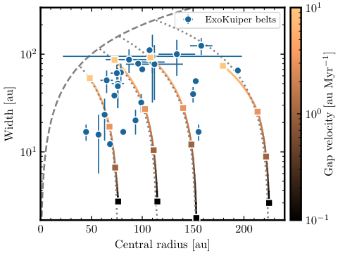
Here we aim to put our findings into the context by comparing our simulation results with the width and radius of exoKuiper belts around FGK stars (defined here as L⊙) as measured by the the ALMA REASONS survey (Matra et al. in prep). Figure 11 shows in blue the observed width and radius including uncertainties. This sample of exoKuiper belts has a median central radius of 95 au, width of 54 au, and a fractional width of 0.63. The coloured squares show the width and radius of planetesimal belts as a function of gap velocity (0, 10, 30 and 100% of the nominal speed), with gap positions of 60, 90, 120 and 180 au and . Given our findings of §4.7, we kept the gaps stationary for 2 Myr for gaps starting at 60 and 90 au, and for 3 Myr for gaps starting at 120 and 180 au in order to be able to form planetesimals at large radii. This waiting period results in an outer edge position that is independent of the gap velocity (very close to the grey dotted lines that represent a fixed outer edge position). For the gaps starting at 120 and 180 au, we evolved them for 10 Myr, and for the gaps starting at 60 and 90 au, we evolved them for 6.3 and 8.6 Myr as they reach the inner boundary before 10 Myr.
This comparison shows that the spread of widths could be achieved by different gap velocities (or different periods over which a gap migrates), and the spread in radius by different initial locations where planetesimals started forming. Overall, we find that all these belts are wider than the width achieved by the gaps moving at 10% the nominal speed (1 au Myr-1), and thus simulations with would not be capable of reproducing the large widths. Similarly, to reproduce the widest belts with widths of au, gaps need to travel at 100% of the nominal speed (10 au Myr-1) or even faster if discs live shorter timescales. In order to reproduce the median values for the radius and width of exoKuiper belts, the gap should start at roughly 90 au and travel at au Myr-1. Therefore, we conclude that the scenario presented in this paper can reproduce the main characteristics (radius and width) of exoKuiper belts.
Note that the apparent correlation between the widths and radii of observed exoKuiper belts is simply due to an upper limit on the width of a belt. Namely, a belt cannot have a width that is twice its central radius (dashed line). In fact, narrow belts are found in belts with both small and large central radius. Similarly, the anti correlation between the width and radius shown by the solid lines is simply a result of a fixed initial gap position. Finally, while we showed that the large spread in the central radius of exoKuiper belts could be obtained by starting the gap at different locations, reproducing the radius distribution is, however, beyond the scope of this paper. In addition to the large spread in radii, the radius distribution of exoKuiper belts is known to be a function of stellar luminosity (Matrà et al. 2018), with belts being on average larger around more luminous and massive stars. Therefore, not only the large spread in radii needs to be explained, but also its dependence on its host star. This dependency could be related to how protoplanetary disks are as well on average larger and contain more dust around more massive stars (Andrews et al. 2013; Pascucci et al. 2016; Andrews et al. 2018a), and to where dust traps are more likely to form.
.
4.9 Outward migrating dust trap
Finally, we explored a dust trap migrating outward. While inward migration is what is mostly expected if the gap was caused by a planet undergoing type II migration, there are special cases where the dust trap could be moving outward. One of such cases is the scenario in which two massive planets are locked in the 3:2 resonance, leading to an outward migration mantaining the 3:2 resonance (Masset & Snellgrove 2001; Crida et al. 2009). Under especial circumstances, single massive planets can also migrate outwards (Masset & Papaloizou 2003; Crida & Morbidelli 2007; Pepliński et al. 2008; Lin & Papaloizou 2012; Dempsey et al. 2021, e.g.), although these cases might be inconsistent with our assumption of an axisymmetric disc. It could also be the case that the dust traps are caused by mechanisms that do not involve the presence of planets, and that these could migrate as discs evolve. For example, if the dust trap is linked to non-ideal MHD effects (Flock et al. 2015), its location could move outwards due to the viscous spreading on a viscous timescale. The dead-zone outer edge is particularly sensitive to the radial profile of the gas surface density (Dzyurkevich et al. 2013, Delage et al. 2021 submitted), and thus this location could move outwards as the disc viscously spreads. Therefore, for completeness we decide to explore the outward migrating case even though it might be unlikely. We simulated the prime case gap starting at 30 au and travelling at the nominal (opposite) velocity for 10 Myr. Figure 12 shows the gas, dust and planetesimal surface densities along with the resulting belt characteristics. Note that the very small crinkles appearing at > 80 au are a numerical artefact.
The planetesimal surface density magnitude decays over time, due to the decreasing availability of dust at higher disc radii and the past planetesimal formation. The resulting belt is actually the widest of all our results, simply because initially planetesimals form rapidly at the closer central position of 30 au, and unlike in the other prime case simulations, the gap does not run into the inner simulated disc radius of 10 au but can migrate outward for the full simulation time of 10 Myr.
An outward migrating gap might not necessarily lead to a wide planetesimal belt if the gap is produced by a planet. An outward migrating planet would sweep the planetesimals that have formed exterior to its orbit, either accreting or scattering them to larger or smaller radii. Depending on the migration speed, planetesimal surface density and presence of inner planets, planetesimal scattering could enhance or slow down its migration (Ida et al. 2000; Kirsh et al. 2009; Morrison & Kratter 2018). However, planetesimal scattering could as well widen the planetesimal belt as scattered planetesimals are implanted onto larger or smaller radii (Walsh et al. 2011, e.g.).
5 Conclusions
In this work we have explored how migrating dust traps in protoplanetary discs can lead to the creation of wide planetesimal belts, serving as a first step to link exoKuiper belts and rings in protoplanetary discs. Using the state-of-the-art dust evolution software DustPy, we investigated the initial conditions most favourable to planetesimal formation for a stationary dust trap, and extended this model to a migrating trap. The main findings of this paper are summarised below.
- 1.
Planetesimal formation is most favourable in low viscosity () discs with steep dust traps close to the central star to maximise dust trapping and trigger the streaming instability. We find these conditions are superior at forming planetesimals in both efficiency and timescale.
- 2.
If the initial disc and trap conditions are favourable to planetesimal formation, dust can still effectively accumulate and form planetesimals as the trap migrates. This leads to a positive correlation between the inward radial speed and resulting planetesimal belt width.
- 3.
If the initial disc and gap conditions are not favourable for a stationary dust trap, we find that moving the trap did not improve these conditions and planetesimal formation remained inefficient.
- 4.
The large widths of observed belts constrain to values at tens of au, if 50 au wide planetesimal belts are indeed formed by migrating dust traps over 10 Myr and not external effects reducing the gas surface density (e.g. photoevaporation). Traps in discs move too slowly to form wide planetesimal belts due to the proportionality between and inward radial velocity. Wider discs or shorter migration timescales would require even higher values of .
- 5.
The large spread in the widths and radii of exoKuiper belts could be due to different trap migration speeds (or protoplanetary disc lifetimes) and different starting locations, respectively.
Acknowledgements
We would like to thank Yuhito Shibaike for a very thorough and constructive review of the paper that improved its quality and clarity. We would also like to thank Mario Flock for providing valuable comments. The work presented in this paper began as a summer student project at the Max Planck Institute for Astronomy, and EM and SM would like to thank the institute for facilitating the internship program. Thanks is also extended to the MPIA IT department for continued access and support with the CPU cluster. SM is supported by a Junior Research Fellowship from Jesus College, University of Cambridge. PP acknowledges support provided by the Alexander von Humboldt Foundation in the framework of the Sofja Kovalevskaja Award endowed by the Federal Ministry of Education and Research. SS and TB acknowledge funding from the European Research Council (ERC) under the European Union’s Horizon 2020 research and innovation programme under grant agreement No 714769 and funding by the Deutsche Forschungsgemeinschaft (DFG, German Research Foundation) under Germany’s Excellence Strategy - EXC-2094 - 390783311 and under Ref no. FOR 2634/1.
Data Availability
The data underlying this article will be shared on reasonable request to the corresponding author. DustPy is available at https://stammler.github.io/dustpy/.
References
- Andrews et al. (2013) Andrews S. M., Rosenfeld K. A., Kraus A. L., Wilner D. J., 2013, ApJ, 771, 129
- Andrews et al. (2018a) Andrews S. M., Terrell M., Tripathi A., Ansdell M., Williams J. P., Wilner D. J., 2018a, ApJ, 865, 157
- Andrews et al. (2018b) Andrews S. M., et al., 2018b, ApJ, 869, L41
- Baruteau et al. (2014) Baruteau C., et al., 2014, in Beuther H., Klessen R. S., Dullemond C. P., Henning T., eds, Protostars and Planets VI. p. 667 (arXiv:1312.4293), doi:10.2458/azu_uapress_9780816531240-ch029
- Birnstiel et al. (2010) Birnstiel T., Dullemond C. P., Brauer F., 2010, A&A, 513, A79
- Blum & Wurm (2000) Blum J., Wurm G., 2000, Icarus, 143, 138
- Booth et al. (2017) Booth M., et al., 2017, MNRAS, 469, 3200
- Brauer et al. (2008) Brauer F., Dullemond C. P., Henning T., 2008, A&A, 480, 859
- Carrera et al. (2017) Carrera D., Gorti U., Johansen A., Davies M. B., 2017, ApJ, 839, 16
- Carrera et al. (2021) Carrera D., Simon J. B., Li R., Kretke K. A., Klahr H., 2021, AJ, 161, 96
- Cieza et al. (2021) Cieza L. A., et al., 2021, MNRAS, 501, 2934
- Crida & Morbidelli (2007) Crida A., Morbidelli A., 2007, MNRAS, 377, 1324
- Crida et al. (2009) Crida A., Masset F., Morbidelli A., 2009, ApJ, 705, L148
- Daley et al. (2019) Daley C., et al., 2019, ApJ, 875, 87
- Dempsey et al. (2021) Dempsey A. M., Muñoz D. J., Lithwick Y., 2021, arXiv e-prints, p. arXiv:2105.05277
- Dipierro et al. (2015) Dipierro G., Price D., Laibe G., Hirsh K., Cerioli A., Lodato G., 2015, MNRAS, 453, L73
- Dong et al. (2017) Dong R., Li S., Chiang E., Li H., 2017, ApJ, 843, 127
- Drążkowska et al. (2016) Drążkowska J., Alibert Y., Moore B., 2016, A&A, 594, A105
- Drążkowska et al. (2021) Drążkowska J., Stammler S. M., Birnstiel T., 2021, A&A, 647, A15
- Dullemond & Penzlin (2018) Dullemond C. P., Penzlin A. B. T., 2018, A&A, 609, A50
- Dullemond et al. (2018) Dullemond C. P., et al., 2018, ApJ, 869, L46
- Dzyurkevich et al. (2013) Dzyurkevich N., Turner N. J., Henning T., Kley W., 2013, ApJ, 765, 114
- Ercolano et al. (2017) Ercolano B., Jennings J., Rosotti G., Birnstiel T., 2017, MNRAS, 472, 4117
- Eriksson et al. (2020) Eriksson L. E. J., Johansen A., Liu B., 2020, A&A, 635, A110
- Eriksson et al. (2021) Eriksson L. E. J., Ronnet T., Johansen A., 2021, A&A, 648, A112
- Faramaz et al. (2019) Faramaz V., et al., 2019, AJ, 158, 162
- Fedele et al. (2010) Fedele D., van den Ancker M. E., Henning T., Jayawardhana R., Oliveira J. M., 2010, A&A, 510, A72
- Fernandez & Ip (1984) Fernandez J. A., Ip W.-H., 1984, Icarus, 58, 109
- Flaherty et al. (2015) Flaherty K. M., Hughes A. M., Rosenfeld K. A., Andrews S. M., Chiang E., Simon J. B., Kerzner S., Wilner D. J., 2015, ApJ, 813, 99
- Flaherty et al. (2017) Flaherty K. M., et al., 2017, ApJ, 843, 150
- Flaherty et al. (2020) Flaherty K., et al., 2020, ApJ, 895, 109
- Flock et al. (2015) Flock M., Ruge J. P., Dzyurkevich N., Henning T., Klahr H., Wolf S., 2015, A&A, 574, A68
- Gárate et al. (2020) Gárate M., Birnstiel T., Drążkowska J., Stammler S. M., 2020, A&A, 635, A149
- Gomes et al. (2004) Gomes R. S., Morbidelli A., Levison H. F., 2004, Icarus, 170, 492
- Gundlach & Blum (2015) Gundlach B., Blum J., 2015, ApJ, 798, 34
- Gundlach et al. (2018) Gundlach B., et al., 2018, MNRAS, 479, 1273
- Haisch et al. (2001) Haisch Karl E. J., Lada E. A., Lada C. J., 2001, ApJ, 553, L153
- Ida et al. (2000) Ida S., Bryden G., Lin D. N. C., Tanaka H., 2000, ApJ, 534, 428
- Jiang & Ormel (2021) Jiang H., Ormel C. W., 2021, MNRAS, 505, 1162
- Johansen et al. (2007) Johansen A., Oishi J. S., Mac Low M.-M., Klahr H., Henning T., Youdin A., 2007, Nature, 448, 1022
- Johansen et al. (2009) Johansen A., Youdin A., Klahr H., 2009, ApJ, 697, 1269
- Kennedy et al. (2018) Kennedy G. M., Marino S., Matrà L., Panić O., Wilner D., Wyatt M. C., Yelverton B., 2018, MNRAS, 475, 4924
- Kirsh et al. (2009) Kirsh D. R., Duncan M., Brasser R., Levison H. F., 2009, Icarus, 199, 197
- Klahr & Schreiber (2020) Klahr H., Schreiber A., 2020, ApJ, 901, 54
- Kley & Nelson (2012) Kley W., Nelson R. P., 2012, ARA&A, 50, 211
- Lenz et al. (2019) Lenz C. T., Klahr H., Birnstiel T., 2019, ApJ, 874, 36
- Lenz et al. (2020) Lenz C. T., Klahr H., Birnstiel T., Kretke K., Stammler S., 2020, A&A, 640, A61
- Li & Youdin (2021) Li R., Youdin A., 2021, arXiv e-prints, p. arXiv:2105.06042
- Li et al. (2009) Li H., Lubow S. H., Li S., Lin D. N. C., 2009, ApJ, 690, L52
- Lin & Papaloizou (1979) Lin D. N. C., Papaloizou J., 1979, MNRAS, 186, 799
- Lin & Papaloizou (1986) Lin D. N. C., Papaloizou J., 1986, ApJ, 309, 846
- Lin & Papaloizou (2012) Lin M.-K., Papaloizou J. C. B., 2012, MNRAS, 421, 780
- Long et al. (2018) Long F., et al., 2018, ApJ, 869, 17
- Lorén-Aguilar & Bate (2015) Lorén-Aguilar P., Bate M. R., 2015, MNRAS, 453, L78
- Lynden-Bell & Pringle (1974) Lynden-Bell D., Pringle J. E., 1974, MNRAS, 168, 603
- MacGregor et al. (2017) MacGregor M. A., et al., 2017, ApJ, 842, 8
- MacGregor et al. (2019) MacGregor M. A., et al., 2019, ApJ, 877, L32
- Marino et al. (2018) Marino S., et al., 2018, MNRAS, 479, 5423
- Marino et al. (2019) Marino S., Yelverton B., Booth M., Faramaz V., Kennedy G. M., Matrà L., Wyatt M. C., 2019, MNRAS, 484, 1257
- Marino et al. (2020) Marino S., et al., 2020, MNRAS, 498, 1319
- Masset & Papaloizou (2003) Masset F. S., Papaloizou J. C. B., 2003, ApJ, 588, 494
- Masset & Snellgrove (2001) Masset F., Snellgrove M., 2001, MNRAS, 320, L55
- Matrà et al. (2018) Matrà L., Marino S., Kennedy G. M., Wyatt M. C., Öberg K. I., Wilner D. J., 2018, ApJ, 859, 72
- Meru et al. (2019) Meru F., Rosotti G. P., Booth R. A., Nazari P., Clarke C. J., 2019, MNRAS, 482, 3678
- Michel et al. (2021) Michel A., van der Marel N., Matthews B., 2021, arXiv e-prints, p. arXiv:2104.05894
- Morrison & Kratter (2018) Morrison S. J., Kratter K. M., 2018, MNRAS, 481, 5180
- Musiolik & Wurm (2019) Musiolik G., Wurm G., 2019, ApJ, 873, 58
- Musiolik et al. (2016) Musiolik G., Teiser J., Jankowski T., Wurm G., 2016, ApJ, 827, 63
- Nazari et al. (2019) Nazari P., Booth R. A., Clarke C. J., Rosotti G. P., Tazzari M., Juhasz A., Meru F., 2019, MNRAS, 485, 5914
- Nederlander et al. (2021) Nederlander A., et al., 2021, arXiv e-prints, p. arXiv:2101.08849
- Ormel & Cuzzi (2007) Ormel C. W., Cuzzi J. N., 2007, A&A, 466, 413
- Pascucci et al. (2016) Pascucci I., et al., 2016, ApJ, 831, 125
- Pepliński et al. (2008) Pepliński A., Artymowicz P., Mellema G., 2008, MNRAS, 387, 1063
- Pérez et al. (2019) Pérez S., Casassus S., Baruteau C., Dong R., Hales A., Cieza L., 2019, AJ, 158, 15
- Pfalzner et al. (2014) Pfalzner S., Steinhausen M., Menten K., 2014, ApJ, 793, L34
- Pinilla et al. (2012) Pinilla P., Benisty M., Birnstiel T., 2012, A&A, 545, A81
- Pinilla et al. (2016) Pinilla P., Flock M., Ovelar M. d. J., Birnstiel T., 2016, A&A, 596, A81
- Pinilla et al. (2021) Pinilla P., Lenz C. T., Stammler S. M., 2021, A&A, 645, A70
- Pinte et al. (2016) Pinte C., Dent W. R. F., Ménard F., Hales A., Hill T., Cortes P., de Gregorio-Monsalvo I., 2016, ApJ, 816, 25
- Pringle (1981) Pringle J. E., 1981, ARA&A, 19, 137
- Ribas et al. (2015) Ribas Á., Bouy H., Merín B., 2015, A&A, 576, A52
- Saito & Sirono (2011) Saito E., Sirono S.-i., 2011, ApJ, 728, 20
- Schoonenberg et al. (2018) Schoonenberg D., Ormel C. W., Krijt S., 2018, A&A, 620, A134
- Sellek et al. (2020) Sellek A. D., Booth R. A., Clarke C. J., 2020, MNRAS, 492, 1279
- Sepulveda et al. (2019) Sepulveda A. G., et al., 2019, ApJ, 881, 84
- Shakura & Sunyaev (1973) Shakura N. I., Sunyaev R. A., 1973, A&A, 500, 33
- Shibaike & Alibert (2020) Shibaike Y., Alibert Y., 2020, A&A, 644, A81
- Smoluchowski (1916) Smoluchowski M. V., 1916, Zeitschrift fur Physik, 17, 557
- Stammler et al. (2019) Stammler S. M., Drążkowska J., Birnstiel T., Klahr H., Dullemond C. P., Andrews S. M., 2019, ApJ, 884, L5
- Steinpilz et al. (2019) Steinpilz T., Teiser J., Wurm G., 2019, ApJ, 874, 60
- Strubbe & Chiang (2006) Strubbe L. E., Chiang E. I., 2006, ApJ, 648, 652
- Takahashi & Inutsuka (2014) Takahashi S. Z., Inutsuka S.-i., 2014, ApJ, 794, 55
- Teague et al. (2016) Teague R., et al., 2016, A&A, 592, A49
- Teague et al. (2018a) Teague R., Bae J., Bergin E. A., Birnstiel T., Foreman-Mackey D., 2018a, ApJ, 860, L12
- Teague et al. (2018b) Teague R., et al., 2018b, ApJ, 864, 133
- Teague et al. (2018c) Teague R., Bae J., Birnstiel T., Bergin E. A., 2018c, ApJ, 868, 113
- Teague et al. (2019) Teague R., Bae J., Bergin E. A., 2019, Nature, 574, 378
- Throop & Bally (2005) Throop H. B., Bally J., 2005, ApJ, 623, L149
- Uribe et al. (2011) Uribe A. L., Klahr H., Flock M., Henning T., 2011, ApJ, 736, 85
- Villenave et al. (2020) Villenave M., et al., 2020, A&A, 642, A164
- Wada et al. (2009) Wada K., Tanaka H., Suyama T., Kimura H., Yamamoto T., 2009, ApJ, 702, 1490
- Wada et al. (2011) Wada K., Tanaka H., Suyama T., Kimura H., Yamamoto T., 2011, ApJ, 737, 36
- Walsh et al. (2011) Walsh K. J., Morbidelli A., Raymond S. N., O’Brien D. P., Mandell A. M., 2011, Nature, 475, 206
- Whipple (1972) Whipple F. L., 1972, in Elvius A., ed., From Plasma to Planet. p. 211
- Youdin & Goodman (2005) Youdin A. N., Goodman J., 2005, ApJ, 620, 459
- Youdin & Lithwick (2007) Youdin A. N., Lithwick Y., 2007, Icarus, 192, 588
- Zhang et al. (2018) Zhang S., et al., 2018, ApJ, 869, L47
Appendix A Surface Density Profile
Appendix B Mass Evolution
The mass evolution of the system for the stationary and migrating gap simulations are shown in Figure 14 and Figure 15 respectively. See §3 for the corresponding discussion.
Appendix C Dust Mass Distribution
The dust (particle) mass distribution of the system at the final epoch for the stationary and migrating gap simulations are shown in Figure 16 and Figure 17 respectively.

