IUEP-HEP-21-02
Yukawa Alignment Revisited in the Higgs Basis
Abstract
We implement a comprehensive and detailed study of the alignment of Yukawa couplings in the so-called Higgs basis taking the framework of general two Higgs doublet models (2HDMs). We clarify the model input parameters and derive the Yukawa couplings considering the two types of CP-violating sources: one from the Higgs potential and the other from the three complex alignment parameters . We consider the theoretical constraints from the perturbative unitarity and for the Higgs potential to be bounded from below as well as the experimental ones from electroweak precision observables. Also considered are the constraints on the alignment parameters from flavor-changing decays, , , and the radiative decay. By introducing the basis-independent Yukawa delay factor , we scrutinize the alignment of the Yukawa couplings of the lightest Higgs boson to the SM fermions.
I Introduction
Since the discovery of the 125 GeV Higgs boson in 2012 at the LHC Aad:2012tfa; Chatrchyan:2012ufa, it has been inspected very closely and extensively. At the early stage, several model-independent studies Carmi:2012yp; Azatov:2012bz; Espinosa:2012ir; Klute:2012pu; Carmi:2012zd; Low:2012rj; Giardino:2012dp; Ellis:2012hz; Espinosa:2012im; Carmi:2012in; Banerjee:2012xc; Bonnet:2012nm; Plehn:2012iz; Djouadi:2012rh; Dobrescu:2012td; Cacciapaglia:2012wb; Belanger:2012gc; Moreau:2012da; Corbett:2012dm; Corbett:2012ja; Masso:2012eq; Cheung:2013kla; Cheung:2014noa show that there were some rooms for it to be unlike the one predicted in the Standard Model (SM) but, after combining all the LHC Higgs data at 7 and 8 TeV Khachatryan:2016vau and especially those at 13 TeV ATLAS:2018uso; Sirunyan:2018ouh; ATLAS:2018bsg; CMS:2018mmw; ATLAS:2018gcr; CMS:2018xuk; Aaboud:2018zhk; CMS:2018lkl; Sirunyan:2018kst; ATLAS:2018lur; CMS:2018nqp; Aaboud:2018urx; Aaboud:2017jvq; Aaboud:2017rss; Sirunyan:2018shy; Sirunyan:2018ygk; Sirunyan:2018mvw; Sirunyan:2018koj; Aad:2019mbh, it turns out that it is best described by the SM Higgs boson. Specifically, the third-generation Yukawa couplings have been established. And the most recent model-independent study Cheung:2018ave shows that the error of the top-quark Yukawa coupling is about 6% while those of the bottom-quark and tau-lepton ones are about 10%. 11 1 Throughout this work, we are using the results presented in Ref. Cheung:2018ave which are based on global fits of the Higgs boson couplings to all the LHC Higgs data at 7 TeV, 8 TeV, and 13 TeV available up to the Summer 2018, corresponding to integrated luminosities per experiment of approximately 5/fb at 7 TeV, 20/fb at 8 TeV and up to 80/fb at 13 TeV. We note that there are more datasets at 13 TeV up to 139/fb and 137/fb collected with the ATLAS and CMS experiments, respectively, see Refs. ATLAS:2020qdt; CMS:2020gsy. Though, without a combined ATLAS and CMS analysis, it is difficult to say conclusively how much the full 13-TeV dataset improves the measurements of Higgs boson properties quantitatively, we observe that the errors are reduced by the amount of about 30% by comparing the results presented in Ref. ATLAS:2020qdt with those in Ref. Aad:2019mbh in which the dataset up to 80/fb is used. In addition, the possibility of negative top-quark Yukawa coupling has been completely ruled out and the bottom-quark Yukawa coupling shows a preference of the positive sign 22 2 Precisely speaking, here the sign of the bottom-quark Yukawa coupling is relative to the top-quark Yukawa coupling configured through the - and -quark loop contributions to the vertex. at about level. For the tau-Yukawa coupling, the current data still do not show any preference for its sign yet. On the other hand, the coupling to a pair of massive vector bosons is constrained to be consistent with the SM value within about 5% at level.
Even though we have not seen any direct hint or evidence of new physics beyond the SM (BSM), we are eagerly anticipating it with various compelling motivations such as the tiny but non-vanishing neutrino masses, matter dominance of our Universe and its evolution driven by dark energy and dark matters, etc Khlopov:2021xnw. In many BSM models, the Higgs sector is extended and it results in existence of several neutral and charged Higgs bosons. Their distinctive features depending on new theoretical frameworks could be directly probed through their productions and decays at future high-energy and high-precision experiments Gunion:1989we; Gunion:1992hs; Carena:2002es; Djouadi:2005gi; Djouadi:2005gj; Accomando:2006ga; Eriksson:2009ws; Dittmaier:2011ti; Dittmaier:2012vm; Heinemeyer:2013tqa; deFlorian:2016spz; Dawson:2013bba; Spira:1997dg; Spira:2016ztx; Dawson:2018dcd; Choi:2021nql.
By the alignment of the Yukawa couplings in general 2HDMs Lee:1973iz; Lee:1974jb; Peccei:1977hh; Fayet:1974fj; Inoue:1982ej; Flores:1982pr; Gunion:1984yn; Botella:1994cs; Branco:1999fs; Branco:2011iw, first of all, we imply that the Yukawa matrices describing the couplings of the two Higgs doublets to the SM fermions should be aligned in the flavor space to avoid the tree-level Higgs-mediated flavor-changing neutral current (FCNC). In 2HDMs, there are three neutral Higgs bosons and one of them should be identified as the observed one at the LHC which weighs 125.5 GeV Sirunyan:2020xwk. In this case, by the alignment of the Yukawa couplings, we also mean that the couplings of this SM-like Higgs boson to the SM fermions should be the same as those of the SM Higgs boson itself or its couplings are strongly constrained to be very SM-like by the current LHC data as outlined above. One of the popular ways to achieve this alignment is to identify the lightest neutral Higgs boson as the 125.5 GeV one and assume that all the other Higgs bosons are heavier or much heavier than the lightest one Haber:1989xc; Gunion:2002zf. But this decoupling scenario is not phenomenologically interesting and another scenario is suggested in which all the couplings of the SM-like Higgs candidate are (almost) aligned with those of the SM Higgs while the other Higgs bosons are not so heavy Craig:2013hca; Carena:2013ooa; Dev:2014yca; Bernon:2015qea.
The alignment of Yukawa couplings are previously discussed and studied Carena:2013ooa; Carena:2014nza. For some recent works, see, for example, Refs. Grzadkowski:2018ohf; Kanemura:2020ibp; Low:2020iua; Li:2020dbg. In this work, taking the framework of general 2HDMs, we implement a comprehensive and detailed study of the alignment of Yukawa couplings in the so-called Higgs basis Donoghue:1978cj; Georgi:1978ri; Botella:1994cs; Branco:1999fs; Davidson:2005cw; Haber:2006ue; Boto:2020wyf in which only the doublet containing the SM-like Higgs boson develops the non-vanishing vacuum expectation value (vev) . For the alignment of the Yukawa matrices, we assume that the Yukawa matrices are aligned in the flavor space Manohar:2006ga; Pich:2009sp; Penuelas:2017ikk by introducing the three alignment parameters with for the couplings to the up-type quarks, the down-type quarks, and the charged leptons, respectively. Under this assumption, there are no Higgs-mediated FCNC couplings at tree level and, at higher orders, they are very suppressed Pich:2009sp; Penuelas:2017ikk; Jung:2010ik; Braeuninger:2010td; Bijnens:2011gd. And then, we identify the lightest neutral Higgs boson as the 125.5 GeV one and consider the alignment of its Yukawa couplings as the masses of the heavier Higgs bosons increase or as the heavy Higgs bosons decouple. We configure that the decoupling of the Yukawa couplings of the lightest Higgs boson is delayed by the amount of compared to its coupling to a pair of massive vector bosons, . We observe that the Yukawa delay factor can be sizable even when if is significantly larger than . We consider the upper limit on from and , and, for and , we demonstrate that they are constrained to be small by the precision LHC Higgs data unless the so-called wrong-sign alignment of the Yukawa couplings Gunion:2002zf; Ferreira:2014naa; Ferreira:2014dya; Biswas:2015zgk; Coyle:2018ydo occurs. 33 3 In the wrong-sign alignment limit, the Yukawa couplings are equal in strength but opposite in sign to the SM ones. Note that the Yukawa delay factor is basis-independent and can be used even when some of the Higgs potential parameters and/or all of the three alignment parameters are complex.
We emphasize that we are reconsidering the decoupling behavior of the Yukawa couplings in the light of the new basis-independent measure of the Yukawa delay factor taking the aligned 2HDM in the Higgs basis. In the Higgs basis, contrasting to the relatively well-known basis, it is easier to understand the analytic structure of intercorrelations among the model parameters. On the other hand, in the aligned 2HDM, there are three uncorrelated complex alignment parameters which provide further CP-violating sources in addition to those in the Higgs potential. The aligned 2HDM accommodates the conventional four types of 2HDMs as the limiting cases when the alignment parameters are real and fully correlated.
This paper is organized as follows. Section II is devoted to a brief review of the 2HDM Higgs potential, the mixing among neutral Higgs bosons and their couplings to the SM particles in the Higgs basis. In Section III, we elaborate on the constraints from the perturbative unitarity, the Higgs potential bounded from below, and the electroweak precision observables as well as the flavor constraints on the alignment parameters. And we carry out numerical analysis of the constraints and the alignment of Yukawa couplings in Section IV. A brief summary and conclusions are made in Section V.
II Two Higgs Doublet Model in the Higgs Basis
In this section, we study the two Higgs doublet model taking the so-called Higgs basis Donoghue:1978cj; Georgi:1978ri; Botella:1994cs; Branco:1999fs; Davidson:2005cw; Haber:2006ue; Boto:2020wyf. We consider the general potential containing 3 dimensionful quadratic and 7 dimensionless quartic parameters, of which four parameters are complex. We closely examine the relations among the potential parameters, Higgs-boson masses, and the neutral Higgs-boson mixing so as to figure out the set of input parameters to be used in the next Section. We further work out the Yukawa couplings in the Higgs basis together with the interactions of the neutral and charged Higgs bosons with massive gauge bosons.
II.1 Higgs Potential
The general 2HDM scalar potential containing two complex SU(2)L doublets of and with the same hypercharge may be given by Choi:2021nql 44 4 In contrast with the Higgs basis which has been taken for this work, we address it as the basis.
| (1) | |||||
in terms of 2 real and 1 complex dimensionful quadratic couplings and 4 real and 3 complex dimensionless quartic couplings. Note that the symmetry under and is hardly broken by the non-vanishing quartic couplings and and, in this case, we have three rephasing-invariant CP-violating phases in the potential. With the general parameterization of two scalar doublets as
| (2) |
and denoting and with , one may remove , , and from the 2HDM potential using three tadpole conditions:
| (3) |
with the square of the charged Higgs-boson mass
| (4) |
On the other hand, in the Higgs basis where only one doublet contains the non-vanishing vev , the general 2HDM scalar potential again contains three (two real and one complex) massive parameters and four real and three complex dimensionless quartic couplings and it might take the same form as in the basis:
| (5) | |||||
where the new complex SU(2)L doublets of and are given by the linear combinations of and as follows
with the relations
| (12) |
in terms of and in Eq. (2). Incidentally, we have that , , and . Note that only the neutral component of the doublet develops the non-vanishing vacuum expectation value and it contains only one physical degree of freedom let alone the Goldstone modes. In the so-called decoupling limit, take over the role of the SM SU(2)L doublet and the remaining three Higgs states are accommodated only by the doublet. 55 5 For a numerical study later, the notations of , , and are taken in the decoupling limit.
The potential parameters and in the Higgs basis could be related to those in the basis through:
| (13) |
for two real and one complex dimensionful parameters and 66 6 We find that our results are consistent with those presented in, for example, Ref. Kanemura:2020ibp.
| (14) | |||||
for four real and three complex dimensionless parameters with . We note that , , and is invariant under the exchanges , , , . The tadpole conditions in the Higgs basis, which are much simpler than those in the basis as shown in Eq. (3), are
| (15) |
where the first condition comes from and the second one from and . Note that the second condition relates the two complex parameters of and .
II.2 Masses, Mixing, and Potential Parameters in the Higgs Basis
In the Higgs basis, the 2HDM Higgs potential includes the mass terms which can be cast into the form consisting of two parts
| (16) |
in terms of the charged Higgs bosons , two neutral scalars , and one neutral pseudoscalar . The charged Higgs boson mass is given by
| (17) |
while the mass-squared matrix of the neutral Higgs bosons takes the form
| (18) |
where and the real and symmetric mass-squared matrix is given by
Note that the quartic couplings and have nothing to do with the masses of Higgs bosons and the mixing of the neutral ones. They can be probed only through the cubic and quartic Higgs self-couplings, see Eq. (5) while noting that only the doublet contains the vev GeV. We further note that decouples from the mixing with the other two neutral states of and in the limit, and its mass squared is simply given by which gives . And, in this decoupling limit of , the CP-violating mixing between the two states of and is dictated only by .
Once the real and symmetric mass-squared matrix is given, the orthogonal mixing matrix is defined through 77 7 Note that we reserve the notations of for the mass eigenstates of three neutral Higgs bosons taking account of CP-violating mixing in the neutral Higgs-boson sector when . In general, the neutral Higgs bosons do not carry definite CP parities and they become mixtures of CP-even and CP-odd states.
| (23) |
such that with the increasing ordering of , if necessary. Note that the mass-squared matrix involves only the four (two real and two complex) quartic couplings once and are given. And then, using the matrix relation , one may find the following expressions for the quartic couplings of in terms of the three masses of neutral Higgs bosons and the components of the orthogonal mixing matrix : 88 8 The orthogonal mixing matrix contains three independent degrees of freedom represented by the three rotation angles.
| (24) | |||||
for given and .
Now we are ready to consider the input parameters for 2HDM in the Higgs basis. First of all, the input parameters for the Higgs potential Eq. (5) are
| (25) |
Using the tadpole conditions in Eq. (15), the dimensionful parameters and can be removed from the set in favor of and observing that the quartic couplings and do not contribute to the mass terms, one may consider the following set of input parameters
| (26) |
where we trade the quartic coupling with the charged Higgs mass using the relation with given. Further using and instead of , we end up with the following set of input parameters:
| (27) |
which contains 12 real degrees of freedom. If desirable, one may remove the unphysical massive parameter in favor of the dimensionless quartic coupling by having an alternative set
| (28) |
consisting of 12 real parameters as well.
For example, in the CP-conserving (CPC) case with , one may denote the masses of the three neutral Higgs bosons by , , and or . Note that is for the SM Higgs boson in the decoupling limit of . The mixing matrix can be parameterized as
| (29) |
introducing the mixing angle between the two CP-even states and . In this CP-conserving case, the relations Eq. (II.2) simplify into
| (30) |
We observe that, in the decoupling limit of , and , and and are determined by the mass differences of and , respectively. Finally, for the study of the CPC case, one may choose one of the following two equivalent sets:
| (31) |
each of which contains 9 real degrees of freedom, and the convention of without loss of generality resulting in and if GeV.
In the presence of non-vanishing and/or , the mixing between the two CP-even states and the CP-odd one arises leading to CP violation in the neutral Higgs sector. By introducing a rotation , 99 9 Or, equivalently, . we note that the Higgs potential given by Eq. (5) is invariant under the following phase rotations:
| (32) |
Considering the tadpole conditions Eq. (15), this might imply that one of the CP phases of , , and can be rotated away by rephasing the Higgs fields . By keeping as an independent input and taking either or , one may use the following set of input parameters: 1010 10 In this CP-violating (CPV) case, we parameterize the mixing matrix by introducing the three mixing angles of , , and as explicitly shown in Eq. (II.2).
| (33) |
which contains 11 real degrees of freedom. In this case, the mixing angle () can be fixed by solving or when and () are given. More explicitly, using the relations in Eq. (II.2), we have
| (34) | |||||
parameterizing the mixing matrix as follow:
Assuming 0 and, for example, taking and as the input mixing angles, the remaining mixing angle is determined by
| (49) |
imposing . If is imposed instead, is determined by
| (50) |
Of course, using instead of , one may use the alternative set
| (51) |
Incidentally, one may choose the basis in which by taking the following set of input parameters:
| (52) |
where all the three mixing angles are independent from one another and is real.
In passing, we note that, in the limit of and , the mixing matrix takes the simpler form
When and , the lightest is SM like and the heavier ones are mostly arbitrary mixtures of and . On the other hand, when and , the lightest is mostly CP odd () and () is SM like when ().
II.3 Yukawa Couplings in Higgs basis
In the 2HDM, the Yukawa couplings might be given by Pich:2009sp
| (57) |
in terms of the six Yukawa matrices with the electroweak eigenstates , , , , and . The two Higgs doublets in the Higgs basis are given by Eq. (II.1):
| (58) |
and their SU(2)-conjugated doublets by
| (59) |
The Yukawa interactions include the following mass terms
| (60) |
which involve only the Yukawa matrices of . Therefore, introducing two unitary matrices relating the left/right-handed electroweak eigenstates to the left/right-handed mass eigenstates with as follows
| (61) |
we have, for the mass terms,
| (62) |
where the three diagonal matrices are
| (63) |
in terms of the six quark and three charged-lepton masses. We note that is nothing but the CKM matrix and, by the use of it, the SU(2)L quark doublets in the electroweak basis can be related to those in the mass basis in the following two ways:
| (64) |
The first relation is used for the Yukawa interactions with the right-handed up-type quarks and the second one for those with the right-handed down-type quarks. Incidentally, we also have
| (65) |
by defining with no physical effects in the case with vanishing neutrino masses.
Collecting all the parameterizations, unitary rotations, and re-parameterizations, the couplings of the neutral Higgs bosons to two fermions are given by
| (66) | |||||
where three Hermitian and three anti-Hermitian Yukawa coupling matrices are
| (67) |
with given in terms of the Yukawa matrix and two unitary matrices as
| (68) |
We observe that the couplings of the field are diagonal in the flavor space and their sizes are directly proportional to the masses of the fermions to which it couples. In contrast, those of the and fields are not diagonal in the flavor space leading to the tree-level Higgs-mediated FCNC and their magnitudes are arbitrary in principle.
To avoid the tree-level FCNC, the matrices are desired to be diagonal which can be achieved by requiring Pich:2009sp 1111 11 Under this requirement, the Yukawa matrix for the Higgs field is indeed diagonal with its diagonal components being proportional to the hierarchical fermion masses multiplied by the common factor , see Eq. (70). For an alternative Yukawa alignment in which can couple to light fermions sizably while still achieving the absence of tree-level FCNCs, see Ref. Egana-Ugrinovic:2019dqu.
| (69) |
along with introducing the three complex alignment parameters . In this case, the two aligned Yukawa matrices and can be diagonalized simultaneously and the Yukawa matrices describing the couplings of and fields to the fermion mass eigenstates are given by
| (70) |
which leads to the Hermitian and anti-Hermitian Yukawa matrices
| (71) |
When , the conventional 2HDMs based on the Glashow-Weinberg condition Glashow:1976nt can be obtained by choosing as shown in Table 1. Otherwise, the couplings of the mass eigenstates of the neutral Higgs bosons to two fermions are given by
| (72) |
with the scalar and pseudoscalar couplings given by
| (73) |
where the upper and lower signs are for the up-type fermions and the down-type fermions , respectively. The simultaneous existence of the scalar and pseudoscalar couplings for a specific signals the CP violation in the neutral Higgs sector. We figure out that there are two different sources of the neutral Higgs-sector CP violation: one is the CP-violating mixing among the CP-even and CP-odd states arising in the presence of non-vanishing in the Higgs potential and the other one is the complex alignment parameters of ’s. Note that the second source is absent in the conventional four types of 2HDMs since ’s are real in those models.
| 2HDM I | 2HDM II | 2HDM III | 2HDM IV | |
|---|---|---|---|---|
The couplings of charged Higgs bosons to two fermions are given by
| (74) |
in terms of the CKM matrix and the Yukawa matrices .
Previously, we note that the Higgs potential given by Eq. (5) is invariant under the phase rotation if the complex potential parameters are accordingly rephased, see Eq. (32). This observation extends to the Yukawa interactions, Eq. (57), by noting that they are invariant under the phase rotations:
| (75) |
Under the alignment assumption given by Eq. (69), the above rephasing invariant rotations become
| (76) |
in terms of the complex alignment parameters. Then one may be able to show that the scalar and pseudoscalar couplings given by Eq. (II.3) are invariant under the phase rotations given by Eq. (76) as they should be. To be explicit, we first note that, under the phase rotation , the electroweak Higgs basis changes as follow:
| (77) |
which leads to
| (78) |
by observing that and should remain the same, respectively. Under the transformation , the components of the mixing matrix change into
| (79) |
On the other hand, under the rotations given in Eq. (76), one may have
| (80) |
with the upper and lower signs being for the up-type massive fermions and the down-type massive fermions , respectively. Using Eqs. (79) and (80), it is straightforward to show that the scalar and pseudoscalar couplings given by Eq. (II.3) are invariant under the phase rotations of Eq. (76).
To summarize, assuming with being the three complex alignment parameters and combining Eqs. (32) and (76), we note that the Higgs potential and the Yukawa interactions are invariant under the following phase rotations:
| (81) |
which, taking account of the CP odd tadpole condition , lead to five rephasing-invariant CPV phases in total. This leaves us more freedom to choose the input parameters for the Higgs potential other than (33), (51), or (52). For example, one may assign three CPV phases to the Higgs potential and take real and positive definite. In this case, the full set of input parameter is to be
| (82) |
which contains 12 and 5 real degrees of freedom in the Higgs potential and the Yukawa interactions, respectively, with , and being fully complex.
II.4 Interactions with Massive Vector Bosons
The cubic interactions of the neutral and charged Higgs bosons with the massive gauge bosons and are described by the three interaction Lagrangians:
| (83) |
respectively, where , and the normalized couplings , and are given in terms of the neutral Higgs-boson mixing matrix by (note that det for any orthogonal matrix ):
| (84) |
leading to the following sum rules:
| (85) |
On the other hand, the quartic interactions of the neutral and charged Higgs bosons with the massive gauge bosons and and massless photons are given by
| (86) |
with and
| (87) |
with , , and .
III Constraints
In this Section, we consider the perturbative unitarity (UNIT) conditions and those for the Higgs potential to be bounded from below (BFB) to obtain the primary theoretical constraints on the potential parameters or, equivalently, the constraints on the Higgs-boson masses including correlations among them and the mixing among the three neutral Higgs bosons. We further consider the constraints on the Higgs masses and their couplings with vector bosons taking into account the electroweak oblique corrections to the so-called and parameters. We emphasize that all the three types of constraints from the perturbative unitarity, the Higgs potential bounded from below, and the electroweak precision observables (EWPOs) are independent of the basis chosen and working in the Higgs basis does not invoke any restrictions. We also consider the constraints on , , and the product of taking account of the charged Higgs contributions to the flavor-changing decays into light leptons, , , and Jung:2010ik; Jung:2010ab. 1212 12 We refer to, for example, Ref. Crivellin:2013wna for an extensive study of flavor observables in the conventional 2HDMs taking the basis.
III.1 Perturbative Unitarity
For the unitarity conditions, we closely follow Ref. Jurciukonis:2018skr 1313 13 We keep our conventions for the potential parameters. considering the three scattering matrices of which are expressed in terms of the quartic couplings , see also Ref. Kanemura:2015ska. The two real and symmetric scattering matrices and are given by
where and . The row vector is given by
| (93) |
and the real and symmetric matrix by
The third scattering matrix is Hermitian which takes the form of
And then, the unitarity conditions are imposed by requiring that the 11 eigenvalues of the three scattering matrices and the quantity should have their moduli smaller than .
When , the 12 unitarity conditions simplify into
| (102) |
While taking , one may have
| (103) |
Then, by combining them, one may arrive at the following UNIT conditions for individual parameters Jurciukonis:2018skr
| (104) |
III.2 Higgs Potential Bounded-from-below
We consider the following 5 necessary conditions for the most general 2HDM Higgs potential with explicit CP violation to be bounded-from-below in a marginal sense Jurciukonis:2018skr: 1414 14 Denoting the quartic part of the scalar potential as , a marginal stability requirement means that for any direction in field space tending to infinity Branco:2011iw. In contrast, a strong stability requirement is without the equality sign. In this work, we adopt the marginal stability requirement.
| (105) |
Note that though the quartic couplings and have no direct relations to the masses and mixing of Higgs bosons but they are interrelated with the other five quartic couplings of through the UNIT and BFB conditions.
III.3 Electroweak Precision Observables
The electroweak oblique corrections to the so-called , and parameters Peskin:1990zt; Peskin:1991sw provide significant constraints on the quartic couplings of the 2HDM. Fixing which is suppressed by an additional factor 1515 15 Here, denotes some heavy mass scale involved with new physics beyond the Standard Model. compared to and , the and parameters are constrained as follows
| (106) |
with , , , , at , , , , and confidence levels (CLs), respectively. For our numerical analysis, we adopt the 95% CL limits. The central values and their standard deviations are given by 1616 16 See the 2020 edition of the review “10. Electroweak Model and Constraints on New Physics” by J.Erler and A. Freitas in Ref. ParticleDataGroup:2020ssz.
| (107) |
with a strong correlation between and parameters. The electroweak oblique parameters, which are defined to arise from new physics only, are in excellent agreement with the SM values of zero for the reference values of GeV and GeV ParticleDataGroup:2020ssz.
In 2HDM, the and parameters might be estimated using the following expressions Toussaint:1978zm; Lee:2012jn
| (108) | |||||
In this work, we ignore the vertex corrections , , and since the size of the most of the quartic couplings are smaller than and the quantum corrections proportional to might be negligible. Then, we observe that all the relevant couplings are determined by the three physical couplings of since and . The one-loop functions are given by 1717 17 See, for example, Ref.Kanemura:2011sj.
| (109) |
We note that and . 1818 18 Here and after, could be understood as, for example, if necessary. When , neglecting the -dependent vertex correction factors , and , and are symmetric under the exchange and they are identically vanishing when . 1919 19 The and parameters are independent of when .
III.4 Flavor Constraints on the Alignment Parameters
The alignment parameters are constrained by considering the charged Higgs contributions to the low energy observables such as flavor-changing decays, leptonic and semileptonic decays of pseudoscalar mesons, the process, meson mixing, the CPV parameter in meson mixing, and the radiative decay Jung:2010ik. In this work, we consider the flavor constraints on the absolute sizes of , and . Note that we neglect the constraints on the products of the alignment parameters taking account of only the single constraints on the absolute values of , and under the assumption that they are fully independent from each other.
The flavor-changing decays into light leptons provide the following constraint on Jung:2010ik:
| (110) |
at 95% CL. On the other hand, the constraint on may come from the -peak precision observables involving the decay assuming the quantum corrections to the vertex beyond the SM is dominated by the charged Higgs contributions. More explicitly, the ratio is used by neglecting the contributions depending on which are suppressed by the factor compared to those depending on . It turns out that the upper limit on linearly increases with as follow Jung:2010ik:
| (111) |
To be very strict, the above upper limit should be applied only when . The similar while more direct upper limit could be obtained by considering the CPV parameter in meson mixing which depends on only neglecting the masses of the light and quarks. Actually the limit from is slightly stronger than that from by the amount of about 10% Jung:2010ik. In this work, for the upper limit on , we apply the slightly weaker constraint from given by Eq. (111) while considering it valid independently of . In passing, for the processes mediated by box diagrams with exchanges of and/or bosons, we note that the leading Willson coefficients which are not suppressed by the light quark mass depend and . When , one might obtain the similar upper limit on as that from Jung:2010ik.
There is no limit on independently of and/or . But one may extract some interesting information on considering the radiative decay. Numerically, the decay amplitude can be cast into the following form Jung:2010ab; Borzumati:1998tg: 2020 20 Note that the product is the rephasing invariant quantity in our convention, see Eq. (76).
| (112) |
When is negative, the interference with the SM amplitude is always constructive and the product is constrained to be small and, as usual, can be significantly larger (smaller) than 1 only when is very small (large). On the contrary, if is positive, could be large independently of . In this case, a destructive interference occurs and the experimental constraints can be satisfied when
| (113) |
Combining the upper limit on given by Eq. (111), we observe that the destructive interference can always occur when
| (114) |
and . Most generally, allowing to be complex, it turns out that the rough 95% CL upper limit on the absolute value of the product is basically saturated by the relation given by Eq. (113) Jung:2010ik or
| (115) |
For the summary, we present the upper limits on , , and and the lower limit on in Fig. 1.
Before closing this section, we briefly comment on the constraints from the heavy Higgs boson searches carried out at the LHC. The heavy neutral Higgs bosons have been searched through their decays into ATLAS:2017eiz; CMS:2018rmh; Bailey:2020ecs; ATLAS:2020zms, CMS:2018hir, ATLAS:2017snw; CMS:2019rvj; ATLAS:2022ohr, ATLAS:2017jag, ATLAS:2017tlw; ATLAS:2017otj; CMS:2018amk; ATLAS:2020tlo, ATLAS:2017xel; CMS:2019qcx, etc. On the other hand, the charged Higgs boson search channels include the decay modes into ATLAS:2018gfm; CMS:2019bfg, ATLAS:2018ntn; CMS:2020imj; ATLAS:2021upq, CMS:2018dzl, CMS:2015yvc; CMS:2020osd, and ATLAS:2017xel. Basically, the experimental upper limits on the product of the production cross section and the decay rate into a specific search mode have been analyzed to obtain the allowed parameter space of a specific model. For example, the search in the final state excludes the presence of a heavy neutral Higgs with below about 1 TeV at 95% CL in the minimal supersymmetric extension of the SM (MSSM) when, depending on scenarios, and the exclusion contour reaches up to TeV for CMS:2018rmh. While in the aligned 2HDM taken in this work, the Yukawa couplings of the up- and down-type quarks and the charged leptons to heavy Higgs bosons are completely uncorrelated and the interpretation of the experimental limits is much more involved. This is because the three alignment parameters of are independent from each other while all of them are involved in the calculation of the decay rate pertinent to a specific search mode. In principle, one can easily avoid the constraints from, for example, and by taking . But it might be still allowed to have and TeV if one can suppress the branching fraction into by choosing the other alignment parameters of and appropriately. In this respect, a through analysis of the experimental search results in the framework of aligned 2HDM with three independent alignment parameters deserves an independent full consideration. In this work, we simply assume that the parameter space considered in the next Section could be made more or less safe from the LHC constraints from no observation of significant excess in the heavy Higgs boson searches by judiciously manipulating the three alignment parameters which are otherwise uncorrelated.
IV Numerical Analysis
From the relation given in Eq. (II.4) and the expressions for the couplings to the two SM fermions given in Eq. (II.3), one might define the Yukawa delay factor by the amount of which the decoupling of the Yukawa couplings of the lightest Higgs boson is delayed compared to its coupling to a pair of massive vector bosons:
| (116) |
where we use the relation for . We observe that the delay factor defined above is basis-independent and can be generally used even in the CPV case. Anticipating that the impacts on the Yukawa delay factor due to the CP-violating phases of and are redundant, we consider the CP-conserving (CPC) case for our numerical study for simplicity. For a recent global analysis of the aligned CPC 2HDM taking account of several phenomenological constraints as well as theoretical requirements, we refer to Ref. Eberhardt:2020dat but with a caution. 2121 21 In Ref. Eberhardt:2020dat, the authors take for the fitting parameters in addition to the Higgs masses GeV, , , , and the mixing angle . In our notations, they use the set of input parameters of . Comparing to given in Eq. (II.2), we find that the potential parameters and are used more than needed while and are missing in the set. Note that and are entirely fixed when the mixing angle and the three neutral Higgs masses are given, see Eq. (II.2), and the parameter should be included at least because it is independent of the Higgs masses and mixing like as .
IV.1 UNIT and BFB constraints
First of all, we consider the UNIT and BFB constraints. Observing that the two conditions depend only on the quartic couplings , we take the following set of input parameters: 2222 22 To have from Eq. (26), we trade with . Note that the dimensionful parameter is irrelevant for the UNIT and BFB constraints.
| (117) |
In the left panel of Fig. 2, we show the scatter plots of versus (upper left), versus (upper right), versus (lower left), and versus (lower right). The plots are produced by randomly generating the quartic couplings in the set. In each plot, the black points are obtained by imposing only the simplified UNIT conditions of Eqs. (III.1) and (103). The full consideration of the UNIT conditions based on the scattering matrices produces the red points. The results obtained by simultaneously imposing the full UNIT and BFB conditions (UNITBFB) are denoted by the blue points. We find our results are very consistent with those presented in Ref. Jurciukonis:2018skr. After imposing the UNIT and UNITBFB conditions, we note that the normalized distributions of the quartic couplings are no longer flat as shown in the right panel of Fig. 2. As in the left panel, the distributions of the quartic couplings obtained by requiring only the UNIT (red) conditions and the combined UNITBFB conditions are in red and blue, respectively. We note that the smaller and the positive values are preferred by further imposing the BFB conditions in addition to the UNIT ones, see Eq. (III.2).

IV.2 Electroweak constraints
Coming to the electroweak (ELW) constraints, since the oblique corrections are expressed in terms of the masses and couplings of Higgs bosons, it is more natural and convenient to take the following set of input parameters:
| (118) |
referring to Eq. (II.2). In the set, all the massive parameters are physical Higgs masses except GeV. We assume that the neutral state is the lightest Higgs boson and plays the role of the SM Higgs boson in the decoupling limit of by taking GeV Sirunyan:2020xwk. And, for the masses of heavy Higgs bosons, we randomly generate their masses squared between and . For the mixing angle , we take the convention of without loss of generality resulting in and . For the implementation of the UNIT and BFB constraints using the set , we recall the quartic couplings in terms of the Higgs masses and the mixing angle in the CPC case given by Eq. (II.2).
Using the set for the input parameters in the CPC case, the and parameters given by Eq. (108) take the following simpler forms:
| (119) | |||||
ignoring the vertex corrections. We observe that is identically vanishing when and, when , we obtain 2323 23 For , note that .
| (120) | |||||
keeping the leading terms. To obtain Eq. (IV.2) for the approximated expressions of the and parameters, we use
| (121) |
for and
| (122) |
for .

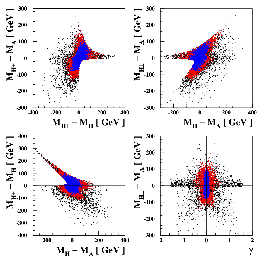
In the left panel of Fig. 3, we show the and parameters imposing the UNIT, BFB, and ELW constraints abbreviated by the combined UNITBFBELW95% ones. Note that the 95% CL ELW limits are adopted and the heavy Higgs masses squared are scanned up to . We find that takes values in the range between and whose absolute values are smaller than , see Eq. (107). Actually, we find that even with only the UNIT and BFB constraints imposed. Note that is mostly negative (positive) when . Specifically, we find that when and . The parameter takes its value between and which are given by the delimited range determined by , the strong correlation and , see Eqs. (106) and (107) and the lower-right plot in the left panel of Fig. 3. Incidentally, we observe that when though it quickly deviates from when . In the right panel of Fig. 3, we show the correlations among the mass differences and the mixing angle using the set . We find that
| (123) |
when 500 GeV (1 TeV).

We show the correlations among the heavy Higgs-boson masses and the mixing angle in the left panel of Fig. 4. Requiring the ELW constraint in addition to the UNITBFB ones, we find that and take values near to 0 and and positive ones more likely, see the right panel of Fig. 4. We find that the UNIT and BFB conditions combined with the ELW constraint restrict the quartic couplings as follows:
| (124) |
IV.3 Alignment of Yukawa couplings
Now, we have come to the point to address the alignment of Yukawa couplings. When we talk about the alignment of the Yukawa couplings in general 2HDMs, we imply: the alignment of them in the flavor space and the alignment of the lightest Higgs-boson couplings to a pair of the SM fermions in the decoupling limit of . By , we precisely mean the assumption that the two Yukawa matrices of and are aligned in the flavor space or , see Eq.(69), which, in the CPC case, leads to
| (125) |
with and for the up- and down-type quarks, respectively, and for the three charged leptons. Then, by , one might mean
| (126) |
In Eq. (125), we note that the quantity is nothing but the coupling which is driven to take the SM value of by the combined UNIT, BFB, and ELW constraints as increases. Therefore, from Eq. (116), the Yukawa delay factor simplifies to , and the alignment of the lightest Higgs-boson couplings to the SM fermions in the decoupling limit is delayed by the amount of which can not be ignored even when if is significantly larger than .


For a quantitative study, in addition to given by Eq. (118), we have added the following set of input parameters containing three real parameters:
| (127) |
In the left panel of Fig. 5, we show the correlations between each of the three alignment parameters and the mixing angle when the absolute value of the corresponding coupling is within 10% range of the SM value of or and for (red) and (blue), respectively. Scanning , near . At , the coupling takes the value of when (red). While if , we note that at (blue). In the right panel of Fig. 5, by the four lines, we show the correlations between and in the four conventional 2HDMs 2424 24 The parameters and are completely uncorrelated in the general 2HDM based on the relation Eq. (69) as shown by the scattered black dots in the right panel of Fig. 5. based on appropriately defined discrete symmetries taking , see Table 1. We observe that both and are bounded only in the type-I 2HDM between and . Otherwise, at least one of them is limitless in principle. Therefore, except the type-I 2HDM, and/or could be largely deviated from 1 in the decoupling limit even when is limited.


To concentrate on the alignment of the lightest Higgs-boson couplings to a pair of the SM fermions in the decoupling limit of under the assumption of as in Eq. (69), we consider a simplified scenario in which the mixing angle is inversely proportional to reflecting the behavior of being suppressed by the quartic powers of the heavy Higgs-boson masses at leading order Choi:2020uum. In the upper-left frame of Fig. 6, we show the scatter plot for versus together with the three curves showing the cases of (black), (red), and (blue) from bottom to top. 2525 25 The choice of is equivalent to fix when and , see Eq. (II.2). The input parameters are the same as in Fig. 4 and the combined UNITBFBELW95% constraints are imposed. For illustration, we take the case of . The coupling of the lightest Higgs boson to a pair of massive vector bosons are constrained by the precision LHC Higgs data Cheung:2018ave. We note that, for example, or can be satisfied when GeV for this choice. We further assume that the masses of the heavy Higgs bosons of , , and are degenerate. This assumption reflects the fact that the combined UNIT BFB ELW95% constraints prefers quite degenerate heavy-Higgs bosons when they weigh more than about 400 GeV as shown in the left panel of Fig. 4. We dub this scenario SCN200 in which we precisely fix and vary the input parameters in the two sets of and as follows:
| (128) | |||||
together with the combined UNIT BFB ELW95% constraints imposed. In this scenario, the Yukawa delay factor is given by
| (129) |
with . Note that we use the approximation in the above equation.
In the upper-right frame of Fig. 6, we show the scatter plot of versus taking SCN200 in which the upper limit on from and is applied, see Eq. (111). We observe that the coupling is within about 30% and 10% ranges of the SM value of when GeV and TeV, respectively. As previously discussed, the alignment of the coupling is delayed by the amount of compared to the coupling and is most deviated from its SM value of by the amount of
| (130) |
To make this point clear, we add the blue and red lines showing taking , and and the magenta one showing . We indeed see that is most close to when and the two lines taking provide the envelope which includes all the scattered points. 2626 26 Note that the line segments for with GeV are located outside the scattered region implying that they are excluded by the upper limit on from and . In the lower frames of Fig. 6, the scatter plots of versus (left) and versus (right) are shown. They are basically the same since and are varied in the same range of . And the same arguments are applied as in the case of : the lines with are most close to among the blue and red lines and those with provide the envelopes which include all the scattered points. We see that and can be largely deviated from their SM values of when is large:
| (131) |
Incidentally, we observe that the constraint on from the flavor-changing decays into light leptons excludes the region with and GeV which is not seen in the window chosen for the scatter plot of versus in Fig. 6, see Eq. (110).

Of course, the alignment parameters are constrained by the precision LHC Higgs data. From the observation that the absolute values of the couplings of the SM-like to a pair of bottom quarks and tau leptons are required to be consistent with within about 10% at level Cheung:2018ave, one might have and . 2727 27 The negative value of is less preferred than the positive one at the level of about considering the -quark loop contributions to the coupling to two gluons Cheung:2018ave. While, for , the current data precision is yet insufficient to tell its sign. In this work, we consider both signs for and . For the positive sign, the condition constrains , see the red points in the left panel of Fig. 7. On the other hand allows the larger values of given by , see the blue points in the left panel of Fig. 7. In the same panel for versus , we also show the lower limit on from through the destructive interference by the magenta lines, see Eq. (114) and the lower-left panel of Fig. 1. We observe that the two regions with are mostly outside the band delimited by the two magenta lines implying that large values of for are hardly constrained by . For , the same arguments are applied, see the right panel of Fig. 7. Note that the constraints from the flavor-changing decays into light leptons given by Eq. (110) are too weak to affect those on by the precision LHC Higgs data.
Lastly, we comment on the wrong-sign alignment limit in the four types of conventional 2HDMs in which the couplings to the down-type quarks and/or those to the charged leptons are equal in strength but opposite in sign to the corresponding SM ones. The two couplings and are completely independent from each other in general 2HDM. But, in the conventional four types of 2HDMs, they are related. We observe that the couplings are given by either or in any type of 2HDMs, see Table 1. In this case, for the value which makes . This implies that, independently of 2HDM type and regardless of the heavy Higgs-mass scale, all four types of 2HDMs could be viable against the LHC Higgs precision data in the wrong-sign alignment limit.
V Conclusions
We have studied the alignment of Yukawa couplings in the framework of general 2HDMs identifying the lightest neutral Higgs boson as the 125 GeV one discovered at the LHC. We take the so-called Higgs basis Donoghue:1978cj; Georgi:1978ri; Botella:1994cs; Branco:1999fs; Davidson:2005cw; Haber:2006ue; Boto:2020wyf for the Higgs potential in which only one of the two doublets contains the non-vanishing vacuum expectation value . For the Yukawa couplings, rather than invoking the Glashow-Weinberg condition Glashow:1976nt based on appropriately defined discrete symmetries, we require the absence of tree-level FCNCs by assuming that the Yukawa matrices describing the couplings of the two Higgs doublets to the SM fermions are aligned in the flavor space Manohar:2006ga; Pich:2009sp; Penuelas:2017ikk.
For a numerical study, we further assume that the seven quartic couplings appearing in the Higgs potential and the three alignment parameters for Yukawa couplings are all real by anticipating that the impacts due to CP-violating phases of and ’s on the alignment of Yukawa couplings are redundant. In this case, in addition to the vev and masses of the SM fermions, the model can be fully described by specifying the following set of 11 free parameters:
where (with ) and denote the masses of CP-even and CP-odd neutral Higgs bosons, respectively, and the mixing between the two CP-even neutral states is described by the angle . The quartic couplings are determined in terms of , , , and . The quartic coupling is related to the massive parameter appearing in the Higgs potential through . On the other hand, the the other quartic couplings and have no direct relevance to the masses and mixing of Higgs bosons. But, we observe that they are interrelated with the other five quartic couplings of through the perturbative unitarity (UNIT) conditions and those for the Higgs potential to be bounded from below (BFB). We note that the UNIT and BFB conditions are basis-independent, i.e., the same in any basis Jurciukonis:2018skr. Also considered are the constraints from the electroweak (ELW) oblique corrections to the and parameters which are expressed in terms of the physical observable quantities of , , and which are again invariant under a change of basis Grzadkowski:2018ohf. We further consider the constraints on the alignment parameters from flavor-changing decays, , , and the radiative decay.
For the independent model parameters and the rephasing invariant combinations of CP-violating phases, among the several points already discussed in the literature, we highlight the following ones:
- 1.
The general 2HDM potential can be fully specified with the masses of the charged and three neutral Higgs bosons, the orthogonal neutral-Higgs boson mixing matrix and the three dimensionless quartic couplings of in addition to the vev .
- 2.
For the CP phases, as far as the Higgs potential and the three complex alignment parameters for the Yukawa couplings are involved, the Lagrangians are invariant under the following phase rotations:
(132) which, taking account of the CP odd tadpole condition , lead to the following five rephasing-invariant CPV phases:
(133) pivoting, for example, around the complex quartic coupling .
Incidentally, it is well known that the 3 alignment parameters are the same in the type-I 2HDM. In this case, they cannot be significantly large than 1 since leads to a non-perturbative top-quark Yukawa coupling and a Landau pole close to the TeV scale. Therefore, in the type-I model among the 4 conventional 2HDMs, all the Yukawa couplings of the lightest Higgs boson most quickly approach the corresponding SM values as the masses of the heavy neutral Higgs bosons increase and their decouplings are least delayed.
We further suggest the following points as the main results specifically pertinent to our analysis:
- 1.
By scanning the heavy Higgs masses up to 1.5 TeV, we find that the UNIT and BFB conditions combined with the ELW constraint restrict the quartic couplings as follows:
(134) And, when 500 GeV (1 TeV), we also find that
(135) - 2.
As the masses of heavy Higgs bosons increase, compared to the coupling of the lightest Higgs boson to a pair of massive vector bosons, the decoupling of the Yukawa couplings to the lightest Higgs boson is delayed by the amount of the Yukawa delay factor which is basis-independent and can be generally used even in the presence of CPV phases. Therefore, though approaches its SM value of 1 very quickly as the masses of heavy Higgs bosons increase, the coupling of to a pair of fermions can significantly deviate from its SM value if is large. Note that is constrained to be small by and , see Eq. (111). While and are constrained to be small by the LHC precision Higgs data when the corresponding Yukawa couplings are with the similar strength and the same sign as the SM ones. But it could be large when the Yukawa coupling takes the wrong sign.
- 3.
The wrong-sign alignment, in which the couplings to a pair of -type fermions are equal in strength but opposite in sign to the corresponding SM ones, occurs when independently of the heavy Higgs-boson masses. In the conventional four types of 2HDMs, or and the Yukawa couplings are given by either or in any type of 2HDMs. We observe that for the value making and any type of conventional 2HDMs is viable against the LHC Higgs precision data.
- 4.
Last but not least, by combining with the upper limit on from and , we derive the lower limit on independently of and when the non-SM contribution to is about two times of the SM one at the amplitude level.
Acknowledgment
We thank Seong Youl Choi for helpful comments on the manuscript. This work was supported by the National Research Foundation (NRF) of Korea Grant No. NRF-2021R1A2B5B02087078 (J.S.L., J.P.). In addition, the work of J.S.L. was supported in part by the NRF of Korea Grant No. NRF-2022R1A5A1030700 and the work of J.P. was supported in part by the NRF of Korea Grant No. NRF-2018R1D1A1B07051126.
References
- (1) G. Aad et al. [ATLAS], “Observation of a new particle in the search for the Standard Model Higgs boson with the ATLAS detector at the LHC,” Phys. Lett. B 716 (2012), 1-29 doi:10.1016/j.physletb.2012.08.020 [arXiv:1207.7214 [hep-ex]].
- (2) S. Chatrchyan et al. [CMS], “Observation of a New Boson at a Mass of 125 GeV with the CMS Experiment at the LHC,” Phys. Lett. B 716 (2012), 30-61 doi:10.1016/j.physletb.2012.08.021 [arXiv:1207.7235 [hep-ex]].
- (3) D. Carmi, A. Falkowski, E. Kuflik and T. Volansky, “Interpreting LHC Higgs Results from Natural New Physics Perspective,” JHEP 07 (2012), 136 doi:10.1007/JHEP07(2012)136 [arXiv:1202.3144 [hep-ph]].
- (4) A. Azatov, R. Contino and J. Galloway, “Model-Independent Bounds on a Light Higgs,” JHEP 04 (2012), 127 [erratum: JHEP 04 (2013), 140] doi:10.1007/JHEP04(2012)127 [arXiv:1202.3415 [hep-ph]].
- (5) J. R. Espinosa, C. Grojean, M. Muhlleitner and M. Trott, “Fingerprinting Higgs Suspects at the LHC,” JHEP 05 (2012), 097 doi:10.1007/JHEP05(2012)097 [arXiv:1202.3697 [hep-ph]].
- (6) M. Klute, R. Lafaye, T. Plehn, M. Rauch and D. Zerwas, “Measuring Higgs Couplings from LHC Data,” Phys. Rev. Lett. 109 (2012), 101801 doi:10.1103/PhysRevLett.109.101801 [arXiv:1205.2699 [hep-ph]].
- (7) D. Carmi, A. Falkowski, E. Kuflik and T. Volansky, “Interpreting the 125 GeV Higgs,” Nuovo Cim. C 035 (2012) no.06, 315-322 doi:10.1393/ncc/i2012-11386-2 [arXiv:1206.4201 [hep-ph]].
- (8) I. Low, J. Lykken and G. Shaughnessy, “Have We Observed the Higgs (Imposter)?,” Phys. Rev. D 86 (2012), 093012 doi:10.1103/PhysRevD.86.093012 [arXiv:1207.1093 [hep-ph]].
- (9) P. P. Giardino, K. Kannike, M. Raidal and A. Strumia, “Is the resonance at 125 GeV the Higgs boson?,” Phys. Lett. B 718 (2012), 469-474 doi:10.1016/j.physletb.2012.10.042 [arXiv:1207.1347 [hep-ph]].
- (10) J. Ellis and T. You, “Global Analysis of the Higgs Candidate with Mass ~ 125 GeV,” JHEP 09 (2012), 123 doi:10.1007/JHEP09(2012)123 [arXiv:1207.1693 [hep-ph]].
- (11) J. R. Espinosa, C. Grojean, M. Muhlleitner and M. Trott, “First Glimpses at Higgs’ face,” JHEP 12 (2012), 045 doi:10.1007/JHEP12(2012)045 [arXiv:1207.1717 [hep-ph]].
- (12) D. Carmi, A. Falkowski, E. Kuflik, T. Volansky and J. Zupan, “Higgs After the Discovery: A Status Report,” JHEP 10 (2012), 196 doi:10.1007/JHEP10(2012)196 [arXiv:1207.1718 [hep-ph]].
- (13) S. Banerjee, S. Mukhopadhyay and B. Mukhopadhyaya, “New Higgs interactions and recent data from the LHC and the Tevatron,” JHEP 10 (2012), 062 doi:10.1007/JHEP10(2012)062 [arXiv:1207.3588 [hep-ph]].
- (14) F. Bonnet, T. Ota, M. Rauch and W. Winter, “Interpretation of precision tests in the Higgs sector in terms of physics beyond the Standard Model,” Phys. Rev. D 86 (2012), 093014 doi:10.1103/PhysRevD.86.093014 [arXiv:1207.4599 [hep-ph]].
- (15) T. Plehn and M. Rauch, “Higgs Couplings after the Discovery,” EPL 100 (2012) no.1, 11002 doi:10.1209/0295-5075/100/11002 [arXiv:1207.6108 [hep-ph]].
- (16) A. Djouadi, “Precision Higgs coupling measurements at the LHC through ratios of production cross sections,” Eur. Phys. J. C 73 (2013), 2498 doi:10.1140/epjc/s10052-013-2498-3 [arXiv:1208.3436 [hep-ph]].
- (17) B. A. Dobrescu and J. D. Lykken, “Coupling spans of the Higgs-like boson,” JHEP 02 (2013), 073 doi:10.1007/JHEP02(2013)073 [arXiv:1210.3342 [hep-ph]].
- (18) G. Cacciapaglia, A. Deandrea, G. Drieu La Rochelle and J. B. Flament, “Higgs couplings beyond the Standard Model,” JHEP 03 (2013), 029 doi:10.1007/JHEP03(2013)029 [arXiv:1210.8120 [hep-ph]].
- (19) G. Belanger, B. Dumont, U. Ellwanger, J. F. Gunion and S. Kraml, “Higgs Couplings at the End of 2012,” JHEP 02 (2013), 053 doi:10.1007/JHEP02(2013)053 [arXiv:1212.5244 [hep-ph]].
- (20) G. Moreau, “Constraining extra-fermion(s) from the Higgs boson data,” Phys. Rev. D 87 (2013) no.1, 015027 doi:10.1103/PhysRevD.87.015027 [arXiv:1210.3977 [hep-ph]].
- (21) T. Corbett, O. J. P. Eboli, J. Gonzalez-Fraile and M. C. Gonzalez-Garcia, “Constraining anomalous Higgs interactions,” Phys. Rev. D 86 (2012), 075013 doi:10.1103/PhysRevD.86.075013 [arXiv:1207.1344 [hep-ph]].
- (22) T. Corbett, O. J. P. Eboli, J. Gonzalez-Fraile and M. C. Gonzalez-Garcia, “Robust Determination of the Higgs Couplings: Power to the Data,” Phys. Rev. D 87 (2013), 015022 doi:10.1103/PhysRevD.87.015022 [arXiv:1211.4580 [hep-ph]].
- (23) E. Massó and V. Sanz, “Limits on anomalous couplings of the Higgs boson to electroweak gauge bosons from LEP and the LHC,” Phys. Rev. D 87 (2013) no.3, 033001 doi:10.1103/PhysRevD.87.033001 [arXiv:1211.1320 [hep-ph]].
- (24) K. Cheung, J. S. Lee and P. Y. Tseng, “Higgs Precision (Higgcision) Era begins,” JHEP 05 (2013), 134 doi:10.1007/JHEP05(2013)134 [arXiv:1302.3794 [hep-ph]].
- (25) K. Cheung, J. S. Lee and P. Y. Tseng, “Higgs precision analysis updates 2014,” Phys. Rev. D 90 (2014), 095009 doi:10.1103/PhysRevD.90.095009 [arXiv:1407.8236 [hep-ph]].
- (26) G. Aad et al. [ATLAS and CMS Collaborations], “Measurements of the Higgs boson production and decay rates and constraints on its couplings from a combined ATLAS and CMS analysis of the LHC pp collision data at and 8 TeV,” JHEP 1608, 045 (2016), [arXiv:1606.02266 [hep-ex]].
- (27) The ATLAS collaboration [ATLAS Collaboration], “Measurements of Higgs boson properties in the diphoton decay channel using 80 fb-1 of collision data at = 13 TeV with the ATLAS detector,” ATLAS-CONF-2018-028.
- (28) A. M. Sirunyan et al. [CMS], “Measurements of Higgs boson properties in the diphoton decay channel in proton-proton collisions at 13 TeV,” JHEP 11 (2018), 185 doi:10.1007/JHEP11(2018)185 [arXiv:1804.02716 [hep-ex]].
- (29) The ATLAS collaboration [ATLAS Collaboration], “Measurements of the Higgs boson production, fiducial and differential cross sections in the decay channel at with the ATLAS detector,” ATLAS-CONF-2018-018.
- (30) CMS Collaboration [CMS Collaboration], “Measurements of properties of the Higgs boson in the four-lepton final state at ,” CMS-PAS-HIG-18-001.
- (31) The ATLAS collaboration [ATLAS Collaboration], “Measurement of gluon fusion and vector boson fusion Higgs boson production cross-sections in the decay channel in pp collisions at TeV with the ATLAS detector,” ATLAS-CONF-2018-004.
- (32) CMS Collaboration [CMS Collaboration], “Measurements of properties of the Higgs boson decaying to a W boson pair in pp collisions at ,” CMS-PAS-HIG-16-042.
- (33) M. Aaboud et al. [ATLAS], “Observation of decays and production with the ATLAS detector,” Phys. Lett. B 786 (2018), 59-86 doi:10.1016/j.physletb.2018.09.013 [arXiv:1808.08238 [hep-ex]].
- (34) CMS Collaboration [CMS Collaboration], “Combined measurements of the Higgs boson’s couplings at TeV,” CMS-PAS-HIG-17-031.
- (35) A. M. Sirunyan et al. [CMS], “Observation of Higgs boson decay to bottom quarks,” Phys. Rev. Lett. 121 (2018) no.12, 121801 doi:10.1103/PhysRevLett.121.121801 [arXiv:1808.08242 [hep-ex]].
- (36) The ATLAS collaboration [ATLAS Collaboration], “Cross-section measurements of the Higgs boson decaying to a pair of tau leptons in proton–proton collisions at TeV with the ATLAS detector,” ATLAS-CONF-2018-021.
- (37) CMS Collaboration [CMS Collaboration], “Search for the standard model Higgs boson decaying to a pair of leptons and produced in association with a W or a Z boson in proton-proton collisions at TeV,” CMS-PAS-HIG-18-007.
- (38) M. Aaboud et al. [ATLAS], “Observation of Higgs boson production in association with a top quark pair at the LHC with the ATLAS detector,” Phys. Lett. B 784 (2018), 173-191 doi:10.1016/j.physletb.2018.07.035 [arXiv:1806.00425 [hep-ex]].
- (39) M. Aaboud et al. [ATLAS Collaboration], “Evidence for the associated production of the Higgs boson and a top quark pair with the ATLAS detector,” Phys. Rev. D 97, no. 7, 072003 (2018), [arXiv:1712.08891 [hep-ex]].
- (40) M. Aaboud et al. [ATLAS], “Search for the standard model Higgs boson produced in association with top quarks and decaying into a pair in collisions at = 13 TeV with the ATLAS detector,” Phys. Rev. D 97 (2018) no.7, 072016 doi:10.1103/PhysRevD.97.072016 [arXiv:1712.08895 [hep-ex]].
- (41) A. M. Sirunyan et al. [CMS], “Evidence for associated production of a Higgs boson with a top quark pair in final states with electrons, muons, and hadronically decaying leptons at 13 TeV,” JHEP 08 (2018), 066 doi:10.1007/JHEP08(2018)066 [arXiv:1803.05485 [hep-ex]].
- (42) A. M. Sirunyan et al. [CMS], “Search for H production in the all-jet final state in proton-proton collisions at 13 TeV,” JHEP 06 (2018), 101 doi:10.1007/JHEP06(2018)101 [arXiv:1803.06986 [hep-ex]].
- (43) A. M. Sirunyan et al. [CMS], “Search for production in the decay channel with leptonic decays in proton-proton collisions at TeV,” JHEP 03 (2019), 026 doi:10.1007/JHEP03(2019)026 [arXiv:1804.03682 [hep-ex]].
- (44) A. M. Sirunyan et al. [CMS], “Combined measurements of Higgs boson couplings in proton–proton collisions at ,” Eur. Phys. J. C 79 (2019) no.5, 421 doi:10.1140/epjc/s10052-019-6909-y [arXiv:1809.10733 [hep-ex]].
- (45) G. Aad et al. [ATLAS], “Combined measurements of Higgs boson production and decay using up to fb-1 of proton-proton collision data at 13 TeV collected with the ATLAS experiment,” Phys. Rev. D 101 (2020) no.1, 012002 doi:10.1103/PhysRevD.101.012002 [arXiv:1909.02845 [hep-ex]].
- (46) K. Cheung, J. S. Lee and P. Y. Tseng, “New Emerging Results in Higgs Precision Analysis Updates 2018 after Establishment of Third-Generation Yukawa Couplings,” JHEP 09 (2019), 098 doi:10.1007/JHEP09(2019)098 [arXiv:1810.02521 [hep-ph]].
- (47) [ATLAS], “A combination of measurements of Higgs boson production and decay using up to fb-1 of proton–proton collision data at 13 TeV collected with the ATLAS experiment,” ATLAS-CONF-2020-027.
- (48) [CMS], “Combined Higgs boson production and decay measurements with up to 137 fb-1 of proton-proton collision data at = 13 TeV,” CMS-PAS-HIG-19-005.
- (49)
For a recent review, see, for example,
M. Khlopov, “What comes after the Standard Model?,” Prog. Part. Nucl. Phys. 116 (2021), 103824 doi:10.1016/j.ppnp.2020.103824 - (50) J. F. Gunion, H. E. Haber, G. L. Kane and S. Dawson, “The Higgs Hunter’s Guide,” Front. Phys. 80 (2000), 1-404 SCIPP-89/13.
- (51) J. F. Gunion, H. E. Haber, G. L. Kane and S. Dawson, “Errata for the Higgs hunter’s guide,” [arXiv:hep-ph/9302272 [hep-ph]].
- (52) M. Carena and H. E. Haber, “Higgs Boson Theory and Phenomenology,” Prog. Part. Nucl. Phys. 50 (2003), 63-152 doi:10.1016/S0146-6410(02)00177-1 [arXiv:hep-ph/0208209 [hep-ph]].
- (53) A. Djouadi, “The Anatomy of electro-weak symmetry breaking. I: The Higgs boson in the standard model,” Phys. Rept. 457 (2008), 1-216 doi:10.1016/j.physrep.2007.10.004 [arXiv:hep-ph/0503172 [hep-ph]].
- (54) A. Djouadi, “The Anatomy of electro-weak symmetry breaking. II. The Higgs bosons in the minimal supersymmetric model,” Phys. Rept. 459 (2008), 1-241 doi:10.1016/j.physrep.2007.10.005 [arXiv:hep-ph/0503173 [hep-ph]].
- (55) E. Accomando, A. G. Akeroyd, E. Akhmetzyanova, J. Albert, A. Alves, N. Amapane, M. Aoki, G. Azuelos, S. Baffioni and A. Ballestrero, et al. “Workshop on CP Studies and Non-Standard Higgs Physics,” doi:10.5170/CERN-2006-009 [arXiv:hep-ph/0608079 [hep-ph]].
- (56) D. Eriksson, J. Rathsman and O. Stal, “2HDMC: Two-Higgs-Doublet Model Calculator Physics and Manual,” Comput. Phys. Commun. 181 (2010), 189-205 doi:10.1016/j.cpc.2009.09.011 [arXiv:0902.0851 [hep-ph]].
- (57) S. Dittmaier et al. [LHC Higgs Cross Section Working Group], “Handbook of LHC Higgs Cross Sections: 1. Inclusive Observables,” doi:10.5170/CERN-2011-002 [arXiv:1101.0593 [hep-ph]].
- (58) S. Dittmaier, C. Mariotti, G. Passarino, R. Tanaka, S. Alekhin, J. Alwall, E. A. Bagnaschi, A. Banfi, J. Blumlein and S. Bolognesi, et al. “Handbook of LHC Higgs Cross Sections: 2. Differential Distributions,” doi:10.5170/CERN-2012-002 [arXiv:1201.3084 [hep-ph]].
- (59) S. Heinemeyer et al. [LHC Higgs Cross Section Working Group], “Handbook of LHC Higgs Cross Sections: 3. Higgs Properties,” doi:10.5170/CERN-2013-004 [arXiv:1307.1347 [hep-ph]].
- (60) D. de Florian et al. [LHC Higgs Cross Section Working Group], “Handbook of LHC Higgs Cross Sections: 4. Deciphering the Nature of the Higgs Sector,” doi:10.2172/1345634, 10.23731/CYRM-2017-002 arXiv:1610.07922 [hep-ph].
- (61) S. Dawson, A. Gritsan, H. Logan, J. Qian, C. Tully, R. Van Kooten, A. Ajaib, A. Anastassov, I. Anderson and D. Asner, et al. “Working Group Report: Higgs Boson,” [arXiv:1310.8361 [hep-ex]].
- (62) M. Spira, “QCD effects in Higgs physics,” Fortsch. Phys. 46 (1998), 203-284 doi:10.1002/(SICI)1521-3978(199804)46:3203::AID-PROP2033.0.CO;2-4 [arXiv:hep-ph/9705337 [hep-ph]].
- (63) M. Spira, “Higgs Boson Production and Decay at Hadron Colliders,” Prog. Part. Nucl. Phys. 95 (2017), 98-159 doi:10.1016/j.ppnp.2017.04.001 [arXiv:1612.07651 [hep-ph]].
- (64) S. Dawson, C. Englert and T. Plehn, “Higgs Physics: It ain’t over till it’s over,” Phys. Rept. 816 (2019), 1-85 doi:10.1016/j.physrep.2019.05.001 [arXiv:1808.01324 [hep-ph]].
- (65) S. Y. Choi, J. S. Lee and J. Park, “Decays of Higgs Bosons in the Standard Model and Beyond,” Prog. Part. Nucl. Phys. 120 (2021), 103880 doi:10.1016/j.ppnp.2021.103880 [arXiv:2101.12435 [hep-ph]].
- (66) T. D. Lee, “A Theory of Spontaneous T Violation,” Phys. Rev. D 8 (1973), 1226-1239 doi:10.1103/PhysRevD.8.1226.
- (67) T. D. Lee, “CP Nonconservation and Spontaneous Symmetry Breaking,” Phys. Rept. 9 (1974), 143-177 doi:10.1016/0370-1573(74)90020-9.
- (68) R. D. Peccei and H. R. Quinn, “CP Conservation in the Presence of Instantons,” Phys. Rev. Lett. 38 (1977), 1440-1443 doi:10.1103/PhysRevLett.38.1440.
- (69) P. Fayet, “A Gauge Theory of Weak and Electromagnetic Interactions with Spontaneous Parity Breaking,” Nucl. Phys. B 78 (1974), 14-28 doi:10.1016/0550-3213(74)90113-8.
- (70) K. Inoue, A. Kakuto, H. Komatsu and S. Takeshita, “Low-Energy Parameters and Particle Masses in a Supersymmetric Grand Unified Model,” Prog. Theor. Phys. 67 (1982), 1889 doi:10.1143/PTP.67.1889.
- (71) R. A. Flores and M. Sher, “Higgs Masses in the Standard, Multi-Higgs and Supersymmetric Models,” Annals Phys. 148 (1983), 95 doi:10.1016/0003-4916(83)90331-7.
- (72) J. F. Gunion and H. E. Haber, “Higgs Bosons in Supersymmetric Models. 1.,” Nucl. Phys. B 272 (1986), 1 [erratum: Nucl. Phys. B 402 (1993), 567-569] doi:10.1016/0550-3213(86)90340-8.
- (73) F. J. Botella and J. P. Silva, “Jarlskog - like invariants for theories with scalars and fermions,” Phys. Rev. D 51 (1995), 3870-3875 doi:10.1103/PhysRevD.51.3870 [arXiv:hep-ph/9411288 [hep-ph]].
- (74) G. C. Branco, L. Lavoura and J. P. Silva, “CP Violation,” Int. Ser. Monogr. Phys. 103 (1999), 1-536, Chapters 22 and 23.
- (75) G. C. Branco, P. M. Ferreira, L. Lavoura, M. N. Rebelo, M. Sher and J. P. Silva, “Theory and phenomenology of two-Higgs-doublet models,” Phys. Rept. 516 (2012), 1-102 doi:10.1016/j.physrep.2012.02.002 [arXiv:1106.0034 [hep-ph]].
- (76) A. M. Sirunyan et al. [CMS], “A measurement of the Higgs boson mass in the diphoton decay channel,” Phys. Lett. B 805 (2020), 135425 doi:10.1016/j.physletb.2020.135425 [arXiv:2002.06398 [hep-ex]].
- (77) H. E. Haber and Y. Nir, “Multiscalar Models With a High-energy Scale,” Nucl. Phys. B 335 (1990), 363-394 doi:10.1016/0550-3213(90)90499-4
- (78) J. F. Gunion and H. E. Haber, “The CP conserving two Higgs doublet model: The Approach to the decoupling limit,” Phys. Rev. D 67 (2003), 075019 doi:10.1103/PhysRevD.67.075019 [arXiv:hep-ph/0207010 [hep-ph]].
- (79) N. Craig, J. Galloway and S. Thomas, “Searching for Signs of the Second Higgs Doublet,” [arXiv:1305.2424 [hep-ph]].
- (80) M. Carena, I. Low, N. R. Shah and C. E. M. Wagner, “Impersonating the Standard Model Higgs Boson: Alignment without Decoupling,” JHEP 04 (2014), 015 doi:10.1007/JHEP04(2014)015 [arXiv:1310.2248 [hep-ph]].
- (81) P. S. Bhupal Dev and A. Pilaftsis, “Maximally Symmetric Two Higgs Doublet Model with Natural Standard Model Alignment,” JHEP 12 (2014), 024 [erratum: JHEP 11 (2015), 147] doi:10.1007/JHEP12(2014)024 [arXiv:1408.3405 [hep-ph]].
- (82) J. Bernon, J. F. Gunion, H. E. Haber, Y. Jiang and S. Kraml, “Scrutinizing the alignment limit in two-Higgs-doublet models: mh=125 GeV,” Phys. Rev. D 92 (2015) no.7, 075004 doi:10.1103/PhysRevD.92.075004 [arXiv:1507.00933 [hep-ph]].
- (83) M. Carena, H. E. Haber, I. Low, N. R. Shah and C. E. M. Wagner, “Complementarity between Nonstandard Higgs Boson Searches and Precision Higgs Boson Measurements in the MSSM,” Phys. Rev. D 91 (2015) no.3, 035003 doi:10.1103/PhysRevD.91.035003 [arXiv:1410.4969 [hep-ph]].
- (84) B. Grzadkowski, H. E. Haber, O. M. Ogreid and P. Osland, “Heavy Higgs boson decays in the alignment limit of the 2HDM,” JHEP 12 (2018), 056 doi:10.1007/JHEP12(2018)056 [arXiv:1808.01472 [hep-ph]].
- (85) S. Kanemura, M. Kubota and K. Yagyu, “Aligned CP-violating Higgs sector canceling the electric dipole moment,” JHEP 08 (2020), 026 doi:10.1007/JHEP08(2020)026 [arXiv:2004.03943 [hep-ph]].
- (86) I. Low, N. R. Shah and X. P. Wang, “Higgs Alignment and Novel CP-Violating Observables in 2HDM,” [arXiv:2012.00773 [hep-ph]].
- (87) S. P. Li, X. Q. Li, Y. Y. Li, Y. D. Yang and X. Zhang, “Power-aligned 2HDM: a correlative perspective on ,” JHEP 01 (2021), 034 doi:10.1007/JHEP01(2021)034 [arXiv:2010.02799 [hep-ph]].
- (88) J. F. Donoghue and L. F. Li, “Properties of Charged Higgs Bosons,” Phys. Rev. D 19 (1979), 945 doi:10.1103/PhysRevD.19.945
- (89) H. Georgi and D. V. Nanopoulos, “Suppression of Flavor Changing Effects From Neutral Spinless Meson Exchange in Gauge Theories,” Phys. Lett. B 82 (1979), 95-96 doi:10.1016/0370-2693(79)90433-7
- (90) S. Davidson and H. E. Haber, “Basis-independent methods for the two-Higgs-doublet model,” Phys. Rev. D 72 (2005), 035004 [erratum: Phys. Rev. D 72 (2005), 099902] doi:10.1103/PhysRevD.72.099902 [arXiv:hep-ph/0504050 [hep-ph]].
- (91) H. E. Haber and D. O’Neil, “Basis-independent methods for the two-Higgs-doublet model. II. The Significance of tan,” Phys. Rev. D 74 (2006), 015018 [erratum: Phys. Rev. D 74 (2006) no.5, 059905] doi:10.1103/PhysRevD.74.015018 [arXiv:hep-ph/0602242 [hep-ph]].
- (92) R. Boto, T. V. Fernandes, H. E. Haber, J. C. Romão and J. P. Silva, “Basis-independent treatment of the complex 2HDM,” Phys. Rev. D 101 (2020) no.5, 055023 doi:10.1103/PhysRevD.101.055023 [arXiv:2001.01430 [hep-ph]].
- (93) A. V. Manohar and M. B. Wise, “Flavor changing neutral currents, an extended scalar sector, and the Higgs production rate at the CERN LHC,” Phys. Rev. D 74 (2006), 035009 doi:10.1103/PhysRevD.74.035009 [arXiv:hep-ph/0606172 [hep-ph]].
- (94) A. Pich and P. Tuzon, “Yukawa Alignment in the Two-Higgs-Doublet Model,” Phys. Rev. D 80 (2009), 091702 doi:10.1103/PhysRevD.80.091702 [arXiv:0908.1554 [hep-ph]].
- (95) A. Peñuelas and A. Pich, “Flavour alignment in multi-Higgs-doublet models,” JHEP 12 (2017), 084 doi:10.1007/JHEP12(2017)084 [arXiv:1710.02040 [hep-ph]].
- (96) M. Jung, A. Pich and P. Tuzon, “Charged-Higgs phenomenology in the Aligned two-Higgs-doublet model,” JHEP 11 (2010), 003 doi:10.1007/JHEP11(2010)003 [arXiv:1006.0470 [hep-ph]].
- (97) C. B. Braeuninger, A. Ibarra and C. Simonetto, “Radiatively induced flavour violation in the general two-Higgs doublet model with Yukawa alignment,” Phys. Lett. B 692 (2010), 189-195 doi:10.1016/j.physletb.2010.07.039 [arXiv:1005.5706 [hep-ph]].
- (98) J. Bijnens, J. Lu and J. Rathsman, “Constraining General Two Higgs Doublet Models by the Evolution of Yukawa Couplings,” JHEP 05 (2012), 118 doi:10.1007/JHEP05(2012)118 [arXiv:1111.5760 [hep-ph]].
- (99) P. M. Ferreira, J. F. Gunion, H. E. Haber and R. Santos, “Probing wrong-sign Yukawa couplings at the LHC and a future linear collider,” Phys. Rev. D 89 (2014) no.11, 115003 doi:10.1103/PhysRevD.89.115003 [arXiv:1403.4736 [hep-ph]].
- (100) P. M. Ferreira, R. Guedes, M. O. P. Sampaio and R. Santos, “Wrong sign and symmetric limits and non-decoupling in 2HDMs,” JHEP 12 (2014), 067 doi:10.1007/JHEP12(2014)067 [arXiv:1409.6723 [hep-ph]].
- (101) A. Biswas and A. Lahiri, “Alignment, reverse alignment, and wrong sign Yukawa couplings in two Higgs doublet models,” Phys. Rev. D 93 (2016) no.11, 115017 doi:10.1103/PhysRevD.93.115017 [arXiv:1511.07159 [hep-ph]].
- (102) N. M. Coyle, B. Li and C. E. M. Wagner, “Wrong sign bottom Yukawa coupling in low energy supersymmetry,” Phys. Rev. D 97 (2018) no.11, 115028 doi:10.1103/PhysRevD.97.115028 [arXiv:1802.09122 [hep-ph]].
- (103) D. Egana-Ugrinovic, S. Homiller and P. R. Meade, “Higgs bosons with large couplings to light quarks,” Phys. Rev. D 100 (2019) no.11, 115041 doi:10.1103/PhysRevD.100.115041 [arXiv:1908.11376 [hep-ph]].
- (104) S. L. Glashow and S. Weinberg, “Natural Conservation Laws for Neutral Currents,” Phys. Rev. D 15 (1977) 1958.
- (105) K. Cheung, J. S. Lee and P. Y. Tseng, “Higgcision in the Two-Higgs Doublet Models,” JHEP 01 (2014), 085 doi:10.1007/JHEP01(2014)085 [arXiv:1310.3937 [hep-ph]].
- (106) M. Jung, A. Pich and P. Tuzon, “The B - Xs gamma Rate and CP Asymmetry within the Aligned Two-Higgs-Doublet Model,” Phys. Rev. D 83 (2011), 074011 doi:10.1103/PhysRevD.83.074011 [arXiv:1011.5154 [hep-ph]].
- (107) A. Crivellin, A. Kokulu and C. Greub, “Flavor-phenomenology of two-Higgs-doublet models with generic Yukawa structure,” Phys. Rev. D 87 (2013) no.9, 094031 doi:10.1103/PhysRevD.87.094031 [arXiv:1303.5877 [hep-ph]].
- (108) D. Jurčiukonis and L. Lavoura, “The three- and four-Higgs couplings in the general two-Higgs-doublet model,” JHEP 12 (2018), 004 doi:10.1007/JHEP12(2018)004 [arXiv:1807.04244 [hep-ph]].
- (109) S. Kanemura and K. Yagyu, “Unitarity bound in the most general two Higgs doublet model,” Phys. Lett. B 751 (2015), 289-296 doi:10.1016/j.physletb.2015.10.047 [arXiv:1509.06060 [hep-ph]].
- (110) M. E. Peskin and T. Takeuchi, “A New constraint on a strongly interacting Higgs sector,” Phys. Rev. Lett. 65 (1990), 964-967 doi:10.1103/PhysRevLett.65.964
- (111) M. E. Peskin and T. Takeuchi, “Estimation of oblique electroweak corrections,” Phys. Rev. D 46 (1992), 381-409 doi:10.1103/PhysRevD.46.381
- (112) P. A. Zyla et al. [Particle Data Group], “Review of Particle Physics,” PTEP 2020 (2020) no.8, 083C01 doi:10.1093/ptep/ptaa104
- (113) D. Toussaint, “Renormalization Effects From Superheavy Higgs Particles,” Phys. Rev. D 18 (1978), 1626 doi:10.1103/PhysRevD.18.1626
- (114) J. S. Lee and A. Pilaftsis, “Radiative Corrections to Scalar Masses and Mixing in a Scale Invariant Two Higgs Doublet Model,” Phys. Rev. D 86 (2012), 035004 doi:10.1103/PhysRevD.86.035004 [arXiv:1201.4891 [hep-ph]].
- (115) S. Kanemura, Y. Okada, H. Taniguchi and K. Tsumura, “Indirect bounds on heavy scalar masses of the two-Higgs-doublet model in light of recent Higgs boson searches,” Phys. Lett. B 704 (2011), 303-307 doi:10.1016/j.physletb.2011.09.035 [arXiv:1108.3297 [hep-ph]].
- (116) F. Borzumati and C. Greub, “2HDMs predictions for anti-B — X(s) gamma in NLO QCD,” Phys. Rev. D 58 (1998), 074004 doi:10.1103/PhysRevD.58.074004 [arXiv:hep-ph/9802391 [hep-ph]].
- (117) M. Aaboud et al. [ATLAS], “Search for additional heavy neutral Higgs and gauge bosons in the ditau final state produced in 36 fb-1 of pp collisions at TeV with the ATLAS detector,” JHEP 01 (2018), 055 doi:10.1007/JHEP01(2018)055 [arXiv:1709.07242 [hep-ex]].
- (118) A. M. Sirunyan et al. [CMS], “Search for additional neutral MSSM Higgs bosons in the final state in proton-proton collisions at 13 TeV,” JHEP 09 (2018), 007 doi:10.1007/JHEP09(2018)007 [arXiv:1803.06553 [hep-ex]].
- (119) A. Bailey [ATLAS and CMS], “Searches for BSM Higgs bosons at ATLAS and CMS,” PoS LHCP2020 (2021), 011 doi:10.22323/1.382.0011
- (120) G. Aad et al. [ATLAS], “Search for heavy Higgs bosons decaying into two tau leptons with the ATLAS detector using collisions at TeV,” Phys. Rev. Lett. 125 (2020) no.5, 051801 doi:10.1103/PhysRevLett.125.051801 [arXiv:2002.12223 [hep-ex]].
- (121) A. M. Sirunyan et al. [CMS], “Search for beyond the standard model Higgs bosons decaying into a pair in pp collisions at 13 TeV,” JHEP 08 (2018), 113 doi:10.1007/JHEP08(2018)113 [arXiv:1805.12191 [hep-ex]].
- (122) M. Aaboud et al. [ATLAS], “Search for Heavy Higgs Bosons Decaying to a Top Quark Pair in Collisions at with the ATLAS Detector,” Phys. Rev. Lett. 119 (2017) no.19, 191803 doi:10.1103/PhysRevLett.119.191803 [arXiv:1707.06025 [hep-ex]].
- (123) A. M. Sirunyan et al. [CMS], “Search for production of four top quarks in final states with same-sign or multiple leptons in proton-proton collisions at 13 TeV,” Eur. Phys. J. C 80 (2020) no.2, 75 doi:10.1140/epjc/s10052-019-7593-7 [arXiv:1908.06463 [hep-ex]].
- (124) [ATLAS], “Search for production in the multilepton final state in proton-proton collisions at TeV with the ATLAS detector,” ATLAS-CONF-2022-008.
- (125) M. Aaboud et al. [ATLAS], “Search for resonance production in final states in collisions at 13 TeV with the ATLAS detector,” JHEP 03 (2018), 042 doi:10.1007/JHEP03(2018)042 [arXiv:1710.07235 [hep-ex]].
- (126) M. Aaboud et al. [ATLAS], “Search for heavy ZZ resonances in the and final states using proton–proton collisions at TeV with the ATLAS detector,” Eur. Phys. J. C 78 (2018) no.4, 293 doi:10.1140/epjc/s10052-018-5686-3 [arXiv:1712.06386 [hep-ex]].
- (127) M. Aaboud et al. [ATLAS], “Searches for heavy and resonances in the and final states in collisions at TeV with the ATLAS detector,” JHEP 03 (2018), 009 doi:10.1007/JHEP03(2018)009 [arXiv:1708.09638 [hep-ex]].
- (128) A. M. Sirunyan et al. [CMS], “Search for a new scalar resonance decaying to a pair of Z bosons in proton-proton collisions at TeV,” JHEP 06 (2018), 127 [erratum: JHEP 03 (2019), 128] doi:10.1007/JHEP06(2018)127 [arXiv:1804.01939 [hep-ex]].
- (129) G. Aad et al. [ATLAS], “Search for heavy resonances decaying into a pair of Z bosons in the and final states using 139 of proton–proton collisions at TeV with the ATLAS detector,” Eur. Phys. J. C 81 (2021) no.4, 332 doi:10.1140/epjc/s10052-021-09013-y [arXiv:2009.14791 [hep-ex]].
- (130) M. Aaboud et al. [ATLAS], “Search for heavy resonances decaying into a or boson and a Higgs boson in final states with leptons and -jets in 36 fb-1 of TeV collisions with the ATLAS detector,” JHEP 03 (2018), 174 [erratum: JHEP 11 (2018), 051] doi:10.1007/JHEP03(2018)174 [arXiv:1712.06518 [hep-ex]].
- (131) A. M. Sirunyan et al. [CMS], “Search for a heavy pseudoscalar boson decaying to a Z and a Higgs boson at 13 TeV,” Eur. Phys. J. C 79 (2019) no.7, 564 doi:10.1140/epjc/s10052-019-7058-z [arXiv:1903.00941 [hep-ex]].
- (132) M. Aaboud et al. [ATLAS], “Search for charged Higgs bosons decaying via in the +jets and +lepton final states with 36 fb-1 of collision data recorded at TeV with the ATLAS experiment,” JHEP 09 (2018), 139 doi:10.1007/JHEP09(2018)139 [arXiv:1807.07915 [hep-ex]].
- (133) A. M. Sirunyan et al. [CMS], “Search for charged Higgs bosons in the H± decay channel in proton-proton collisions at 13 TeV,” JHEP 07 (2019), 142 doi:10.1007/JHEP07(2019)142 [arXiv:1903.04560 [hep-ex]].
- (134) M. Aaboud et al. [ATLAS], “Search for charged Higgs bosons decaying into top and bottom quarks at = 13 TeV with the ATLAS detector,” JHEP 11 (2018), 085 doi:10.1007/JHEP11(2018)085 [arXiv:1808.03599 [hep-ex]].
- (135) A. M. Sirunyan et al. [CMS], “Search for charged Higgs bosons decaying into a top and a bottom quark in the all-jet final state of pp collisions at = 13 TeV,” JHEP 07 (2020), 126 doi:10.1007/JHEP07(2020)126 [arXiv:2001.07763 [hep-ex]].
- (136) G. Aad et al. [ATLAS], “Search for charged Higgs bosons decaying into a top quark and a bottom quark at = 13 TeV with the ATLAS detector,” JHEP 06 (2021), 145 doi:10.1007/JHEP06(2021)145 [arXiv:2102.10076 [hep-ex]].
- (137) A. M. Sirunyan et al. [CMS], “Search for a charged Higgs boson decaying to charm and bottom quarks in proton-proton collisions at TeV,” JHEP 11 (2018), 115 doi:10.1007/JHEP11(2018)115 [arXiv:1808.06575 [hep-ex]].
- (138) V. Khachatryan et al. [CMS], “Search for a light charged Higgs boson decaying to in pp collisions at TeV,” JHEP 12 (2015), 178 doi:10.1007/JHEP12(2015)178 [arXiv:1510.04252 [hep-ex]].
- (139) A. M. Sirunyan et al. [CMS], “Search for a light charged Higgs boson in the H± cs channel in proton-proton collisions at 13 TeV,” Phys. Rev. D 102 (2020) no.7, 072001 doi:10.1103/PhysRevD.102.072001 [arXiv:2005.08900 [hep-ex]].
- (140) O. Eberhardt, A. P. Martínez and A. Pich, “Global fits in the Aligned Two-Higgs-Doublet model,” JHEP 05 (2021), 005 doi:10.1007/JHEP05(2021)005 [arXiv:2012.09200 [hep-ph]].
- (141) S. Y. Choi, J. S. Lee and J. Park, “Alignment of Yukawa couplings in two Higgs doublet models,” [arXiv:2011.04978 [hep-ph]].