Shadow process tomography of quantum channels

We now ask: can the principles of shadow tomography be applied to process tomography? In order to apply the shadow tomography framework to a process $\mathcal{E}$, we make our lives conceptually easier through the use of (the Choi version of) the Choi-Jamiołkowski isomorphism to map a process into a density matrix. Specifically, we specialize to the case of finite dimension, where $\mathcal{E}:\mathcal{C}^{d\times d}\rightarrow\mathcal{C}^{d\times d}$ and is completely positive and trace-preserving. We define the unnormalized, maximally entangled state on a tensor product of two Hilbert spaces $A$ and $B$ each of dimension $d$

(We remark that this state can be prepared by starting in the logical $\left|0\right>_{A}\otimes\left|0\right>_{B}$ state, applying Hadamard to each qubit in the first register, then applying pair-wise CNOTs from the $i$th qubit of the first register to the $i$th qubit of the second register.) We then define the Choi state

We note that $\eta$ is a density matrix (completely positive and of finite trace) up to a normalization factor $d$.

Given a Choi state $\eta$ of dimension $d^{2}\times d^{2}$ and an input density matrix $\rho$ of size $d\times d$, we can find the result of $\mathcal{E}(\rho)$ as

where we have taken the transpose of $\rho$ with respect to the logical basis (that is, the basis in which we defined $\left|\omega\right>$). This has the (simple) interpretation that given a Choi state, we can teleport $\rho$ through $\mathcal{E}$ to find its result, as shown in Fig. 1.

To understand the teleportation interpretation, consider an arbitrary state $\left|\psi\right>_{C}=\sum_{n}c_{n}\left|n\right>$. Starting with $\left|\omega\right>_{AB}\left|\psi\right>_{C}$ and projecting onto $\left|\omega\right>_{BC}$ yields:

Not surprisingly, the Choi state and its recovery of the channel is basis-specific, as the teleportation above makes explicit. However, its operational interpretation–that of state teleportation–we will find useful in applying shadow tomography concepts to process tomography.

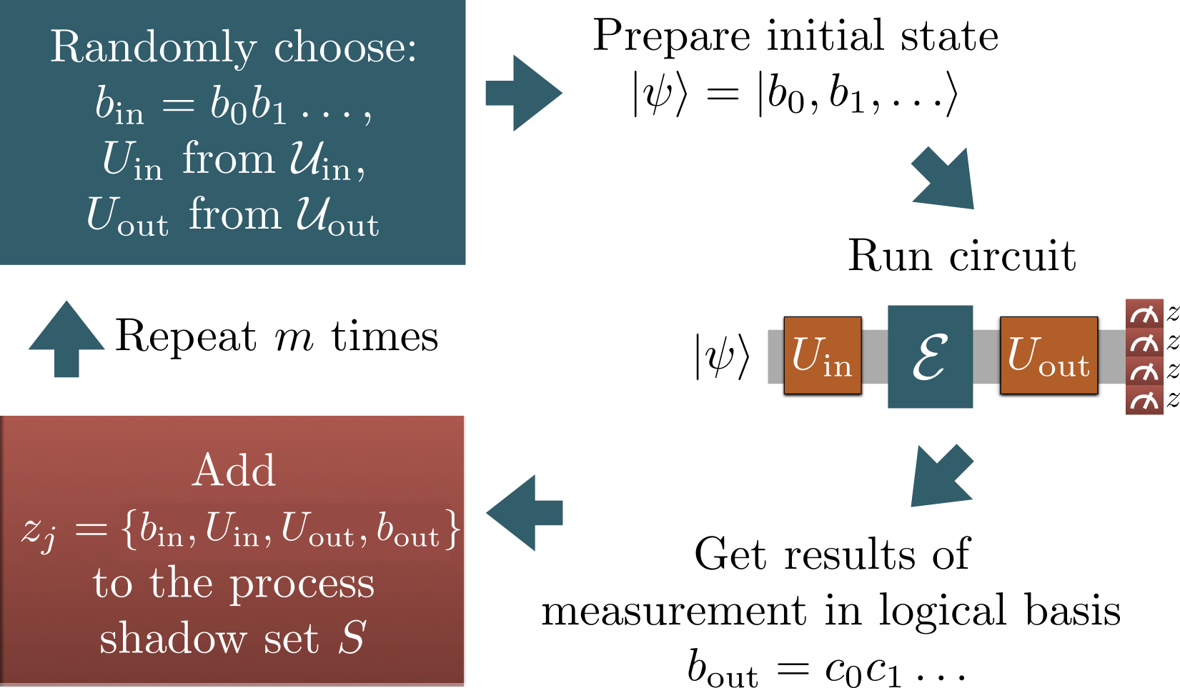
The Choi isomorphism provides a mapping from quantum channels to density matrices. Therefore in theory, we can perform process shadow tomography by applying shadow tomography on the Choi state. However, such a procedure is practically inefficient because we would need to prepare the highly entangled state $\left|\omega\right>$ between two copies of the system. Instead, we use the teleportation interpretation of the Choi isomorphism and implement process shadow tomography using this procedure (see also Fig. 2):

1. 1.

   Uniformly draw a random bit string $b_{\textrm{in}}\in\{0,1\}^{n}$ and prepare $\left|b_{\textrm{in}}\right>$

2. 2.

   Apply an unitary $U_{\textrm{in}}$ drawn randomly from an ensemble $\mathcal{U}_{\textrm{in}}$. In particular, we will consider two possibilities for $\mathcal{U}_{\textrm{in}}$: random single-qubit Pauli rotations ($\mathcal{U}_{\rm P}^{\otimes n}$) and random global Clifford ($\mathcal{U}_{\rm C}$).

3. 3.

   Apply the channel $\mathcal{E}$

4. 4.

   Apply an unitary $U_{\textrm{out}}$ drawn randomly from an ensemble $\mathcal{U}_{\textrm{out}}$, which is not necessary the same as $\mathcal{U}_{\textrm{in}}$. Again, we will consider $\mathcal{U}_{\textrm{out}}=\mathcal{U}_{\rm P}^{\otimes n}$ and $\mathcal{U}_{\textrm{out}}=\mathcal{U}_{\rm C}$

5. 5.

   Measure in the computational basis to obtain a bit string $b_{\textrm{out}}$.

6. 6.

   Add the combination $z=\{b_{\textrm{in}},U_{\textrm{in}},U_{\textrm{out}},b_{\textrm{out}}\}$ to the set $\zeta$ of shadow representations of the Choi state $\eta$ (Eq. 16).

7. 7.

   Repeat the above $m$ times.

Define

We show in Appendix A that the probability of getting a particular combination $z$ can be written as

Then,

is a linear map of the Choi state. If $\mathcal{M}_{\mathcal{U}_{\textrm{in}}\otimes\mathcal{U}_{\textrm{out}}}$ is invertible, we define

as a single-shot shadow of $\eta$ labeled by its parameters $z=\{b_{\textrm{in}},\mathcal{U}_{\textrm{in}},\mathcal{U}_{\textrm{out}},b_{\textrm{out}}\}$. Clearly, taking the expectation over all possible such choices and outcomes for $z$ will yield the original Choi state; that is, $\mathbb{E}_{U_{\textrm{in}},U_{\textrm{out}},b_{\textrm{in}},b_{\textrm{out}}}\hat{\zeta}=\eta$.

Repeating the procedure above for $m$ times, we obtain a collection of $m$ shadows $\hat{\zeta}_{1},\dots,\hat{\zeta}_{m}$. The average of the collection, $\zeta=\frac{1}{m}\sum_{j=1}^{m}\hat{\zeta}_{j}$, provides an estimator for the Choi state $\eta=\lim_{m\rightarrow\infty}\zeta$.

In shadow tomography, an important metric is the sample complexity, i.e. the minimum $m$ such that the estimator is close to correct values. Requiring the distance between the state estimator $\zeta$ and the Choi state $\eta$ to be small is usually too restrictive (The sample complexity would scale polynomially with the Hilbert space dimension). Instead, we only ask that the estimator and the Choi state are close in computing the expectation values of certain observables.

Given a density matrix $\rho$ and an observable $O$, we define $\hat{o}=\textrm{Tr}[\hat{\zeta}\rho^{T}\otimes O]$ as the single-shot estimator of $o=\textrm{Tr}[\mathcal{E}(\rho)O]$. Again, $\mathbb{E}\ \hat{o}=o$, where the mean is taken over all $z$ combinations ($\mathcal{U}_{\textrm{in}},\mathcal{U}_{\textrm{out}},b_{\textrm{in}},$ and $b_{\textrm{out}}$). Considering a collection of $m$ single-shot estimators $\hat{o}_{1},\dots,\hat{o}_{m}$, we define $\tilde{o}(\rho,N,K)$ as the median-of-means estimator, computed by dividing the collection into $K$ subsets, each of size $N=m/K$, and taking the median of the means of the subsets.

Before we prove the sample complexity of process shadow tomography, we would like to note its qualitative differences from state shadow tomography. First, if we were to actually apply state shadow tomography on the Choi state, both $b_{\textrm{in}}$ and $b_{\textrm{out}}$ would have been measurement outcomes and their distributions depend on the Choi state $\eta$. In contrast, $b_{\textrm{in}}$ in our procedure is drawn from an ensemble independent of $\eta$. Effectively, our procedure performs state shadow tomography on the Choi state and post-selects on the first copy of the system being in $\left|b_{\textrm{in}}\right>$. We show in Appendix A that this distinction disappears when we draw $b_{\textrm{in}}$ uniformly.

The second difference between state and process tomography is that the latter allows possibly different choices for $\mathcal{U}_{\textrm{in}}$ and $\mathcal{U}_{\textrm{out}}$. This enables four different mix-and-match scenarios when we restrict the ensembles to either $\mathcal{U}_{\rm C}$ or $\mathcal{U}_{\rm P}^{\otimes n}$. The following theorem, the central result of this work, estimates the sample complexity in the four scenarios, providing an analog of Theorem 1 for process shadow tomography.

Note that $\left\|\mathcal{S}(\rho)\right\|\leq 14$ if $\rho$ is a normalized density matrix and $\left\|\mathcal{S}(O)\right\|\leq 14\ \text{rank}(O)^{2}\left\|O\right\|^{2}$ in general.

We have now established concrete formal bounds for shadow process tomography which are similar in form to those for shadow state tomography. What does this mean for estimating quantities of interest?

One obvious difference between Theorem 2 and the analogous state shadows result is the daunting factor of $4^{n}$ in Eq. 25. Mathematically, this factor of $4^{n}$ follows from the fact that the Choi state of Eq. 16, which takes normalized input states to normalized output states via Eq. 17, has trace $2^{n}$. In significant contrast to the state shadow case, this exponential factor affects even the use of semi-global Clifford measurements when $\rho,O$ in Eq. 28 are rank-1 operators, i.e. state projectors. To explain the reason for the difference, in the state shadows case, if we prepare a (physical, unit trace) Choi state in the lab, the expectation value of the projector $\rho^{T}\otimes O$ can be estimated from randomized measurement with a cost independent of the system size. This total overlap includes a contribution from the exponentially small overlap of the input register state with $\rho^{T}$. By contrast, the expectation value in Eq. 28 corresponds to the probability of finding the channel-evolved state $\mathcal{E}(\rho)$ to be in state $O$; since a physical quantum channel will act without any initial probability of accepting or rejecting the input state, the probability of interest in Eq. 28 is exponentially larger than its physical state analogue.

Next, consider the choice for $\mathcal{U}_{\textrm{in}}$. From Theorem 2, this choice will affect $f_{\mathcal{U}_{\textrm{in}}}(\rho)$. If $\mathcal{U}_{\textrm{in}}=\mathcal{U}_{\rm C}$ and $\rho$ is a normalized density matrix,

is bounded for all $\rho$. On the other hand, if $\mathcal{U}_{\textrm{in}}=\mathcal{U}_{\rm P}^{\otimes n}$, $f_{\mathcal{U}_{\rm P}^{\otimes n}}(\rho)$ grows exponentially with the support size of $\rho$. So unless $\rho$ is supported on only a few sites, we should always choose $\mathcal{U}_{\textrm{in}}=\mathcal{U}_{\rm C}$ over $\mathcal{U}_{\rm P}^{\otimes n}$. Put in other terms, use of $\mathcal{U}_{\rm P}^{\otimes n}$ in the input space means that estimation of the effects of the channel work best on either high temperature states ($\rho$ has a polynomial expansion in local operators in the inverse temperature) or on mostly depolarized inputs (such as most qubits set randomly and only a few polarized). On the other hand, the effects of the channel on highly entangled or highly polarized input states are best determined by using $\mathcal{U}_{\rm C}$ on the input.

Next, for the choice of $\mathcal{U}_{\textrm{out}}$, we note that

Similarly to the state shadow tomography, we would choose

• •

  $\mathcal{U}_{\textrm{out}}=\mathcal{U}_{\rm C}$ if $O$ is a low-rank observable, e.g. the fidelity to a reference state, entanglement witness.

• •

  $\mathcal{U}_{\textrm{out}}=\mathcal{U}_{\rm P}^{\otimes n}$ is $O$ is supported on a few qubits, e.g. local observables.

This becomes subtler and more important as we look to the next section, in which we consider a unique element of shadow process tomography: the ability to compose multiple channels together to create an estimate of the total channel thus developed.

Finally, there is a fundamental difference between the Choi state as concept and the Choi state as actual entangled state sent through a channel. Specifically, the latter case allows all options from shadow tomography. The former case only allows measurements that are not entangled between inputs and outputs. We will not remark on this additional power at this time, other than to say that in quantum sensing and related protocols the additional benefit of having access to the entangled bits can be substantial in, e.g., multiple interaction or applications of the channel for estimation Pirandola et al. 2019.

One possible application of the above would be to estimation of transition probabilities. For transitions between computational-basis eigenstates, say from $\left|i\right>\to\left|f\right>$, this can be done by estimating the expectation value of the projector $O=\left|i\right>\!\left<i\right|\otimes\left|f\right>\!\left<f\right|$ in the Choi state $\eta$. A simple computation gives

where the $M_{a}$ form a Kraus representation for the channel $\mathcal{E}(\rho)=\sum_{a}M_{a}\rho M_{a}^{\dagger}$. If the initial and final states $\left|i,f\right>$ are localized to a small number $k$ qubits and the rest of the system was considered in a high temperature (full mixed) state, then the projector $O$ is a localized operator, and the random Pauli measurements should efficiently predict these transition probabilities. On the other hand, for an initial vacuum plus few excitation state, random Clifford measurements would yield reasonable bounds on estimation.

Ref Huang et al. 2020 notes that the Pauli measurement scheme is well suited for estimating spatial correlation functions, like the two point function $\langle\sigma^{z}_{i}\sigma^{z}_{j}\rangle=\textrm{Tr}[\rho\sigma^{z}_{i}\sigma^{z}_{j}]$ for sites $i$ and $j$. Using shadows, we can extend this to calculation correlation functions in time between local operators: $\textrm{Tr}[\mathcal{E}(\rho A)B]$. Note, however, that the shadow norm squared for this correlation function goes as $4^{k}$ where $k$ is the size of the support of $\rho A\otimes B$. As noted above, this adds a constraint that $\rho$ be composed mostly of low-weight strings. As a result it is useful to turn emphasis away from the initial state and to consider the case $\rho=\mathbb{I}$ and unitary $\mathcal{E}$. In this case we don’t consider the correlation function with respect to a particular state, rather we look learning about how operators evolve in the Heisenberg picture. For a unitary $U$ corresponding to evolution for time $t$ we can estimate functions like

with a sample cost exponential in the support of $A\otimes B$. More details on this application (including to nonunitary channels) can be found in Appendix C.

Shadow tomography is capable of predicting functions which are both linear and non-linear in the quantum state. In particular, Ref. Huang et al. 2020 gives an algorithm for estimating $\rm{tr}(O\rho^{2})$ for an arbitrary operator $O$. This proceeds by finding a linear operator $\tilde{O}$ such that $\textrm{Tr}(O\rho^{2})=\textrm{Tr}(\tilde{O}\rho\otimes\rho)$, where the first trace is on a Hilbert space $\mathcal{H}$ while the second is on $\mathcal{H}\otimes\mathcal{H}$. For example, we can estimate the purity of a state $\rho$ using $O=S$ the SWAP operator, because

Applied to the Choi state of a given channel, this can be used to verify if the channel is unitary, i.e. has a single Kraus operator.

To see this, note that a channel $\mathcal{E}$ is unitary if and only if its Choi state,

is maximally entangled. (To see it in one direction: if $\mathcal{E}$ is unitary, one easily checks that $\eta^{2}=\eta$, up to normalization. The converse is slightly more tedious but straightforward). From the definition, any Choi state has the property that the partial trace over the output system $B$ gives the maximally mixed state for the input system $A$:

Therefore, if the total state $\eta$ is pure up to normalization, $\textrm{Tr}\,\eta^{2}=d^{2}$ (or equivalently $\eta^{2}=d\eta$, where $d={\rm dim}~H_{A}$), then we can conclude that the Choi state is maximally entangled, and thus that the channel $\epsilon$ is unitary.

Unfortunately, the SWAP operator $S$ is completely non-local: $k$ qubits partitioned into two sets of $k/2$ qubits, the SWAP operator acts on all $k$ qubits. Thus according to the estimates in Huang et al. 2020, random Pauli measurements would require a number of samples of order $4^{k}$ to estimate $\textrm{Tr}\,\eta^{2}$. This is the same requirement as doing full process tomography. Random Clifford measurements likewise require a sample size scaling exponentially with the number of qubits. It would be extremely interesting to determine if there exists a measurement set that can produce non-exponential scaling, or to prove that no such set can exist.

This task has two somewhat disparate applications in quantum gravity. One is to the black hole information paradox. The complexity of decoding Hawking radiation to determine the initial, pre-black hole state is believed to be exponential in the logarithm of the Hilbert space dimension Harlow and Hayden 2013. A more basic question is to simply check whether the formation and radiation process produces a unitary channel. In a very different regime, many recent proposals have been made to experimentally determine if Newtonian gravity can entangle meso-to-macroscopic objects in a lab Kafri and Taylor 2013; Bose et al. 2017; Marletto and Vedral 2017; Carney et al. 2019; Carney et al. 2021. Understanding whether the channel generated by the gravitational interaction is unitary or not is crucially important in determining the implications of these experiments Carney 2022. These experiments typically involve just a few low-dimensional systems (e.g., two qubits Bose et al. 2017), and so the above exponential scaling does not present a substantial difficulty.

What if we start with a shadow tomography estimator $\sigma$ to the input state, $\rho_{in}$, which was derived from sampling over $\mathcal{U}_{\rm P}^{\otimes n}$ using shadow state tomography? If we have the estimator for the Choi state $\zeta$ we need to calculate

where the sum is over the set $S_{m}$ and the similar set $R_{k}$ that defines $\sigma$. Note that the transpose operation on $\tau$ simply flips the sign of the $Y$-portion of the Pauli representation, analogous to complex conjugation, for this simple channel example.

Fortunately, summing up over sample pairs is relatively simple, and the final state involves a sum over only the output samples $\nu,c$. This seems like we have a statement that shadows map to shadows. However, unlike our original shadows, this estimator for the output no longer has positive values in front of each $\tau$ product. Let us consider the quasiprobability term:

This points to an interesting future research direction: better understanding the emergence of an (effective) sign problem in the application of a shadow to a shadow; we discuss this in more detail at the end of this section.

Just as we can apply a shadow process to a shadow state, consider what happens if we have process shadows for two channels, $\mathcal{X}$ and $\mathcal{Y}$, each with Choi state shadows $\eta_{X},\eta_{Y}$. Can we construct an approximation to the channel $\mathcal{Y}\circ\mathcal{X}$?

Using the teleportation-based interpretation of the Choi state, it suffices to project onto a maximally entangled state between the output register of $X$, $B$, and the input register of $Y$, $A^{\prime}$. Using the Choi representation of both processes, with set $S_{m}$ of $b,\mu,c,\nu$ values for the first channel and $S_{m^{\prime}}$ of $b^{\prime},\mu^{\prime},c^{\prime},\nu^{\prime}$ values for the second channel, we find immediately

Consider a random variable $s$ drawn uniformly from $S=\{5/2,1/4,1/4,1/4,1/4,-2\}$. We are interested in properties of

This corresponds to composing two $N$-qubit channels with Pauli shadows according to Eqs. Eq. 49, Eq. 50 without any assuming any correlations between qubits. While the signed weights in Eq. 49 point to the existence of a sign problem, we want to investigate how important it is in practice to keep track of weights of small absolute value or of negative sign. First, we can ask what is the probability that $k$ of the $N$ samples are either $5/2$ or $-2$. We get

Then, given that we have $k$ drawn uniformly from $5/2$ and $-2$, we want to know how many $-2$’s we have, and if the overall number is even. The conditional averages are

From this we see that, for $k\geq 1$, we have an equal probability of having an even number of $-2$’s and an odd number of $-2$’s. We also have the average number of $-2$’s is independent of being even or odd and is $k/2$.

The total probability over all $S$ options for having a negative weight (an odd number of $-2$’s) is

What is the total probability of positive? We have the chance that no large values are chosen, $(2/3)^{N}$, and then we have the chance that some number are chosen, in which case we have a 1/2 chance of being positive, giving

as expected.

Thus we conclude that for random states, there is only a slight bias towards positive weights $\pi>0$ as the number of qubits, $N$, becomes large. We can understand this bias as related to the probability of having no $|S|>1$ values at all, e.g., $(2/3)^{N}$. We cannot hope to avoid the sign problem by having only a few negative weights.

However, while the weights are only slightly biased towards being positive, the amplitude of positive states is more heavily biased. We rewrite $\pi=(-1)^{l}A$ where $A>0$, we can look at $a=\log A$ as a random variable, which is correlated with $l\in\{0,1\}$. For $k>0$ large values ($|S|>1$) we have $l$ evenly distributed and $\bar{a}(k)$ corresponds to $(N-k)\log 1/4+\frac{k}{2}\left(\log 5/2+\log 2\right)$. In the large $N$ limit, $a$ becomes normally distributed, which means that returning to the distribution of $|A|$, we have (except for a $(2/3)^{N}$ correction) a log normal distribution with log mean given by averaging $\bar{\bar{a}}=\sum_{k}\bar{a}(k)p_{k}\sim\frac{2N}{3}\log(1/4)+\frac{N}{6}\log 5$ and standard deviation $\sim\sqrt{N/6}\log 5$. The log normal distribution implies that a few, rare values will dominate the overall behavior of the weights. It is then worth investigating whether strategies based on importance sampling can accelerate the process of channel composition.

References

- Gisin and Thew (2007) N. Gisin and R. Thew, Quantum communication, Nat. Photonics 1, 165 (2007).
- Holevo (1973) A. S. Holevo, Bounds for the quantity of information transmitted by quantum communication channel, Probl. Infrom. Transm. 9, 177 (1973).
- Kafri and Taylor (2013) D. Kafri and J. M. Taylor, A noise inequality for classical forces, arXiv e-prints , arXiv:1311.4558 (2013), arXiv:1311.4558 [quant-ph] .
- Bose et al. (2017) S. Bose, A. Mazumdar, G. W. Morley, H. Ulbricht, M. Toroš, M. Paternostro, A. A. Geraci, P. F. Barker, M. S. Kim, and G. Milburn, Spin Entanglement Witness for Quantum Gravity, Phys. Rev. Lett. 119, 240401 (2017), arXiv:1707.06050 [quant-ph] .
- Marletto and Vedral (2017) C. Marletto and V. Vedral, Gravitationally Induced Entanglement between Two Massive Particles is Sufficient Evidence of Quantum Effects in Gravity, Phys. Rev. Lett. 119, 240402 (2017), arXiv:1707.06036 [quant-ph] .
- Carney et al. (2019) D. Carney, P. C. E. Stamp, and J. M. Taylor, Tabletop experiments for quantum gravity: a user’s manual, Class. Quant. Grav. 36, 034001 (2019), arXiv:1807.11494 [quant-ph] .
- Carney et al. (2021) D. Carney, H. Müller, and J. M. Taylor, Using an Atom Interferometer to Infer Gravitational Entanglement Generation, PRX Quantum 2, 030330 (2021), arXiv:2101.11629 [quant-ph] .
- Gross et al. (2010) D. Gross, Y.-K. Liu, S. T. Flammia, S. Becker, and J. Eisert, Quantum state tomography via compressed sensing, Physical Review Letters 105, 150401 (2010), arXiv: 0909.3304.
- Chuang and Nielsen (1997) I. L. Chuang and M. A. Nielsen, Prescription for experimental determination of the dynamics of a quantum black box, Journal of Modern Optics 44, 2455 (1997).
- Branderhorst et al. (2009) M. Branderhorst, J. Nunn, I. Walmsley, and R. Kosut, Simplified quantum process tomography, New Journal of Physics 11, 115010 (2009).
- Shabani et al. (2011) A. Shabani, R. L. Kosut, M. Mohseni, H. Rabitz, M. A. Broome, M. P. Almeida, A. Fedrizzi, and A. G. White, Efficient measurement of quantum dynamics via compressive sensing, Physical review letters 106, 100401 (2011).
- Flammia et al. (2012) S. T. Flammia, D. Gross, Y.-K. Liu, and J. Eisert, Quantum tomography via compressed sensing: error bounds, sample complexity and efficient estimators, New Journal of Physics 14, 095022 (2012), publisher: IOP Publishing.
- Huang et al. (2022) H.-Y. Huang, R. Kueng, G. Torlai, V. V. Albert, and J. Preskill, Provably efficient machine learning for quantum many-body problems, Science 377 (2022).
- Aaronson (2018) S. Aaronson, Shadow tomography of quantum states, in Proceedings of the 50th annual ACM SIGACT symposium on theory of computing (2018) pp. 325–338.
- Huang et al. (2020) H.-Y. Huang, R. Kueng, and J. Preskill, Predicting many properties of a quantum system from very few measurements, Nature Physics 16, 1050 (2020).
- Zhu et al. (2022) D. Zhu, Z. P. Cian, C. Noel, A. Risinger, D. Biswas, L. Egan, Y. Zhu, A. M. Green, C. H. Alderete, N. H. Nguyen, Q. Wang, A. Maksymov, Y. Nam, M. Cetina, N. M. Linke, M. Hafezi, and C. Monroe, Cross-platform comparison of arbitrary quantum states, Nature Communications 13, 6620 (2022), number: 1 Publisher: Nature Publishing Group.
- Struchalin et al. (2021) G. Struchalin, Y. A. Zagorovskii, E. Kovlakov, S. Straupe, and S. Kulik, Experimental Estimation of Quantum State Properties from Classical Shadows, PRX Quantum 2, 010307 (2021).
- Zhang et al. (2021) T. Zhang, J. Sun, X.-X. Fang, X. Zhang, X. Yuan, and H. Lu, Experimental quantum state measurement with classical shadows, arXiv:2106.10190 (2021).
- Surawy-Stepney et al. (2022) T. Surawy-Stepney, J. Kahn, R. Kueng, and M. Guta, Projected least-squares quantum process tomography, Quantum 6, 844 (2022).
- Jamiołkowski (1972) A. Jamiołkowski, Linear transformations which preserve trace and positive semidefiniteness of operators, Reports on Mathematical Physics 3, 275 (1972).
- Choi (1975) M.-D. Choi, Completely positive linear maps on complex matrices, Linear Algebra and its Applications 10, 285 (1975).
- Leung (2003) D. W. Leung, Choi’s proof as a recipe for quantum process tomography, Journal of Mathematical Physics 44, 528 (2003).
- Pirandola et al. (2019) S. Pirandola, R. Laurenza, C. Lupo, and J. L. Pereira, Fundamental limits to quantum channel discrimination, npj Quantum Information 5, 50 (2019).
- Harlow and Hayden (2013) D. Harlow and P. Hayden, Quantum computation vs. firewalls, Journal of High Energy Physics 2013, 85 (2013), arXiv:1301.4504 [hep-th] .
- Carney (2022) D. Carney, Newton, entanglement, and the graviton, Physical Review D 105, 10.1103/physrevd.105.024029 (2022).
- Miszczak et al. (2011) J. A. Miszczak, Z. Puchała, and P. Gawron, QI package for analysis of quantum states and operations (2011), https://github.com/iitis/qi.
- Bansal (2015) H. Bansal, Entanglement Cost Mathematica (2015), https://github.com/hardikbansal/EntanglementCostMathematica.
- Levy et al. (2021) R. Levy, D. Luo, and B. K. Clark, Classical shadows for quantum process tomography on near-term quantum computers, arXiv:2110.02965 (2021).
- Helsen et al. (2021) J. Helsen, M. Ioannou, I. Roth, J. Kitzinger, E. Onorati, A. H. Werner, and J. Eisert, Estimating gate-set properties from random sequences (2021), arXiv:2110.13178 [quant-ph] .
- (30) D. Gross, F. Krahmer, and R. Kueng, A Partial Derandomization of PhaseLift Using Spherical Designs, J Fourier Anal Appl 21, 229.
- Carmichael (1993) H. Carmichael, An open systems approach to quantum optics, Lecture notes in physics No. 18 (Springer-Verlag, Berlin ; New York, 1993).