A phase field crystal theory of the kinematics of dislocation lines
Abstract
We introduce a dislocation density tensor and derive its kinematic evolution law from a phase field description of crystal deformations in three dimensions. The phase field crystal (PFC) model is used to define the lattice distortion, including topological singularities, and the associated configurational stresses. We derive an exact expression for the velocity of dislocation line determined by the phase field evolution, and show that dislocation motion in the PFC is driven by a Peach-Koehler force. As is well known from earlier PFC model studies, the configurational stress is not divergence free for a general field configuration. Therefore, we also present a method (PFCMEq) to constrain the diffusive dynamics to mechanical equilibrium by adding an independent and integrable distortion so that the total resulting stress is divergence free. In the PFCMEq model, the far-field stress agrees very well with the predictions from continuum elasticity, while the near-field stress around the dislocation core is regularized by the smooth nature of the phase-field. We apply this framework to study the rate of shrinkage of an dislocation loop seeded in its glide plane.
1 Introduction
Plasticity in crystalline solids primarily refers to permanent deformations resulting from the nucleation, motion, and interaction of extended dislocations. Classical plasticity theories deal with the yielding of materials within continuum solid mechanics Hill 1998, Wu 2004. Deviations from elastic response are described with additional variables (e.g., the plastic strain), which effectively describe the onset of plasticity (yielding criteria), as well as the mechanical properties of plastically deformed media (e.g., work hardening). A macroscopic description of the collective behavior of dislocation ensembles is thus achieved, usually assuming homogeneous media for large systems. In crystal plasticity, inhomogeneities and anisotropies are accounted for, with the theory having been implemented as a computationally efficient finite element model Roters et al. 2010, Pokharel et al. 2014. These theories are largely phenomenological in nature, and rely on constitutive laws and material parameters to be determined by other methods, or extracted from experiments. They can be finely tuned, but sometimes fail in describing mesoscale effects Rollett et al. 2015. On the other hand, remarkable mesoscale descriptions have been developed by tracking single dislocations Kubin et al. 1992, Bulatov et al. 1998, Sills et al. 2016, Koslowski et al. 2002, Rodney et al. 2003. These approaches typically evolve dislocation lines through Peach-Koehler type forces while incorporating their slip system, mobilities, and dislocation reactions phenomenologically. Stress fields are described within classical elasticity theory Anderson et al. 2017. Since linear elasticity predicts a singular elastic field at the dislocation core, theories featuring its regularization are usually exploited. Prominent examples are the non-singular theory obtained by spreading the Burgers vector isotropically about dislocation lines Cai et al. 2006, and the stress field regularization obtained within a strain gradient elasticity framework Lazar and Maugin 2005. Plastic behavior then emerges when considering systems with many dislocations and proper statistical sampling Devincre et al. 2008. Still, the accuracy and predictive power of these approaches depend on how well dislocations are modeled as isolated objects. In this context, mesoscale theories that require a limited set of phenomenological inputs are instrumental in connecting macroscopic plastic behavior to microscopic features of crystalline materials.
The Phase Field Crystal (PFC) model is an alternative framework to describe the nonequilibrium evolution of defected materials at the mesoscale Elder et al. 2002, Emmerich et al. 2012, Momeni et al. 2018. Within the phase field description, complex processes such as dislocation nucleation Skogvoll et al. 2021b, dislocation dissociation and stacking fault formation Mianroodi and Svendsen 2015, creep Berry et al. 2015, fracture Liu et al. 2020, and boundary driven grain motion Provatas et al. 2007, Wu and Voorhees 2012, Yamanaka et al. 2017, Salvalaglio et al. 2018 have been studied. The phase field allows a short scale regularization of defect core divergences inherent in classical elasticity, while allowing for the treatment of defect topology, grain boundary structures, and associated mobilities. For static studies, the only constitutive input required is the (defect free) equilibrium free energy, functional of the phase field, which has a minimizer that corresponds to a spatially periodic configuration. For time dependent problems, the phase field is generally assumed to obey a gradient flow that minimizes the free energy functional. When topological defects are present in the phase field configuration, their motion directly follows from the gradient flow, without any additional specification of slip systems, stacking fault energies, and line or boundary mobilities. The PFC model thus begins with the definition of a scalar order parameter (or phase field) , function of space and time, so that its equilibrium configuration corresponds to a perfectly periodic, undistorted, configuration. A non-convex free energy functional of the field and its gradients is chosen so that its minimizer has the same spatial symmetry as the lattice of interest Elder et al. 2010. The requisite free energies have been derived by using the methods of density functional theory Elder et al. 2007, Huang et al. 2010, Archer et al. 2019, although our calculations below will rely on modified forms of the classical Brazovskii functional description of modulated phases Brazovskii 1975, also known as the Swift-Hohenberg model in the convection literature Swift and Hohenberg 1977.
Despite the model’s successes to date, a clear connection with classical theory of dislocation motion in crystalline solids is lacking. At its most basic level, the phase field does not carry mass, and hence momentum. Therefore the only stresses (momentum current) that appear in the theory are the reversible contributions that arise from variations of the free energy with respect to distortions of the phase field Skaugen et al. 2018a. Neither momentum currents that arise in a material due to Galilean invariance, nor dissipative currents that would couple directly to the material distortion are present Forster 1975. Unlike classical theories of dislocation motion, the primary object of the model is the phase field, from which other quantities are derived. For an appropriate choice of the free energy functional, the phase field minimizer is a “crystalline" phase in that translational symmetry is broken. As is conventionally the case, the minimizer admits an expansion in a reciprocal space basis set. This expansion is further restricted to include only those wave vector modes in reciprocal space that are critical at onset of the broken symmetry phase. Configurational distortions of the phase field appear as slow (in space and time) modulations of the complex amplitudes of the expansion. A displacement vector is defined from the phase of the modulation. Configurational topological defects are possible and appear as (combinations of) zeros of the complex amplitudes, points at which the phases of the modulation are singular. The corresponding defect current, however, is solely related to the phase field, and to the equation governing its temporal evolution. This is in contrast with more general dislocation density currents in solid mechanics which also include dissipative contributions. An attempt to bridge the PFC description and a field theory of dislocation mechanics has been given in Ref. Acharya and Viñals 2020, where an extended free energy is introduced, which includes a material elastic contribution and the coupling between the two.
Since the theory lacks a proper description of momentum conservation, it also cannot describe the relaxation of elastic excitations. The first attempt at extending the PFC model to include elastic interactions considered a phenomenological second order temporal derivative in the equation of motion for the phase field Stefanovic et al. 2006, which allowed for fast relaxation of short-wavelength elastic disturbances. Later efforts have included coupling the PFC phase field to a velocity field Ramos et al. 2010, or various methods of coarse graining it to develop a consistent hydrodynamical description Tóth et al. 2013, Heinonen et al. 2016. Such approaches are necessary for a proper description of processes where elastic interactions are important, such as crack propagation and defect dynamics. Other efforts have been made to develop efficient modeling approaches in which the time scale of elastic interactions is a priori set to zero , i.e. when mechanical equilibrium is obeyed at all times. The latter approach is justified when deformations are slow, including many of the applications mentioned such as creep and boundary driven grain motion. This approach was first introduced in Ref. Heinonen et al. 2014 which involved relaxing elastic excitations separately and instantaneously within the amplitude equation formulation of the PFC model Goldenfeld et al. 2005. The same strategy was later developed for the PFC model in two dimensional isotropic 2D lattices by adding to the phase-field a correction at each time step that ensured instantaneous mechanical equilibrium Skaugen et al. 2018b, Salvalaglio et al. 2020. In this paper, we present a generalization of this approach to anisotropic crystals in three dimensions (PFC-MEq). Since a distorted phase field configuration determines the corresponding configurational stresses Skaugen et al. 2018a, Skogvoll et al. 2021a, the method yields regularized stress profiles for dislocation lines in three dimensions down to the defect core. In the case of a point defect, it was shown in Ref. Salvalaglio et al. 2020 that the stress field at the core agrees with the predictions of the non-singular theory of Ref. Cai et al. 2006, and with gradient elasticity models Lazar and Maugin 2005, Lazar 2017, indicating that the results obtained here can serve as benchmarks for similar theories in three dimensions. The specific example of a dislocation loop in a bcc lattice is considered, and the far-field stresses given by the field are shown to coincide with predictions by continuum elasticity.
The rest of the paper is structured as follows. In Sec. 2, we introduce the theoretical method used to define topological defects from a periodic -field. This allows us to define a dislocation density tensor in terms of the phase field (Eq. (12)), and obtain the dislocation line velocity (Eq. (16)). These are key results, which are applied in several examples in Sec. 3. First, we use the PFC model to numerically study the shrinkage of a dislocation loop in a bcc lattice. Then, we show analytically that Eq. (16) captures the motion of dislocations driven by a Peach-Koehler type force, and hence by a local stress. Finally, we introduce the PFC-MEq model, and compare the shrinkage of the dislocation loop under PFC and PFC-MEq dynamics. While the results are qualitatively similar for the case of a shear dislocation loop, the constraint of mechanical equilibrium causes the shrinkage to happen much faster. We finally confirm that the stress field derived from the field in the PFC-MEq model agrees with that which would follow from continuum elasticity theory, with the same singular dislocation density as source, and with no adjustable parameters.
2 Kinematics of a dislocation line in three dimensions
Dislocations in 3D crystals are line defects, where each point on the line is characterized by the tangent vector at that point and a Burgers vector , see Figure 1(a).

By introducing a local Cartesian plane normal to , the distance of an arbitrary point to a point on can be decomposed into an in-plane vector and a vector , i.e. . A deformed state can be described by a displacement field and, in the presence of a dislocation, is discontinuous across a surface (branch cut) spanned by the dislocation, given by
| (1) |
where and are the values of the displacement field at each side of the branch cut, respectively. We use the negative sign convention relating the contour integral with the Burgers vector. Here, is a small circuit enclosing the dislocation line in the -plane, directed according to the right-hand rule with respect to . The dislocation density tensor associated with the line is Lazar 2014
| (2) |
where is the component of the Burgers vector of the line, and is the line element in the direction of the line. is a short-hand notation for the delta function, with dimension of inverse area, locating the position of the dislocation line for each component of the dislocation density tensor. It is defined by the line integral over the dislocation line of the full delta function (which scales as inverse volume). The dislocation density tensor is defined so that , where we are using the Einstein summation convention over repeated indices.
In the PFC models, a crystal state is represented by a periodic phase field of a given crystal symmetry. A reference crystalline lattice,
| (3) |
is defined by a set of primary (smallest) reciprocal lattice vectors of length , and higher harmonics , also on the reciprocal lattice but with (see, e.g., with for a bcc lattice in Fig. 1(b)). The lattice constant of the crystal is then given by . This represents a perfect crystal configuration in the absence of defects and distortion, where the average value and the amplitudes are constants. In the phase-field crystal theory presented in Refs. Elder et al. 2002, Elder and Grant 2004, near the solid-liquid transition point, only the terms from the primary reciprocal lattice vectors contribute to , while in general for more sharply peaked density profiles, there are also contributions from the higher order harmonics . For a distorted crystal lattice, the mode amplitudes become complex scalar fields, henceforth named complex amplitudes , such that
| (4) |
In this section, we provide an accurate description of dislocation lines as topological defects in the phase of the complex amplitudes . We generalize the method of tracking topological defects as zeros of a complex order parameter as introduced in Refs. Halperin 1981 and Mazenko 1997, and apply it to accurately derive the kinematics of dislocation lines.
Given a phase field configuration , the complex amplitudes can be found by a demodulation as described in A.1. Decomposing each amplitude , into its modulus and phase , we have that for a perfect lattice, and is constant. Displacing a lattice plane by a slowly varying transforms the phase as . Thus, the phase provides a direct measure of the displacement field relative to the reference lattice, i.e.,
| (5) |
where denotes the -th Cartesian coordinate of . It is possible to invert Eq. (5), and solve for the displacement field as function of the phases and reciprocal vectors. We use the following identity which is valid for lattices with cubic symmetry, where all primary reciprocal lattice vectors have the same length (see B)
| (6) |
so that the displacement is given by
| (7) |
Eq. (7) shows that a dislocation line, which introduces a discontinuity in the displacement field, leads to a discontinuity in the phases . This is the first key insight, which we illustrate in Fig. 2.

By using Eq. (5) and the fact that the Burgers vector is constant along the dislocation line, we relate the Burgers vector to the phase as
| (8) |
where is the (integer) winding number of the phase around the dislocation line. That is an integer follows from the fact that while may have a discontinuity across the branch cut, the complex amplitude is well-defined and continuous everywhere. Therefore the circulation of the phase must be an integer multiple of . By the same reasoning, for an amplitude for which , at the dislocation line, the phase is undefined (singular), so the modulus must go to zero for to remain continuous. This is the second key insight, which allows us to identify the location of the dislocation line with the zeros of the complex amplitudes .
The complex amplitude is isomorphic to a -component vector field . The study of how to track zeros of any dimensional vector field in any dimensions was introduced in Ref. Halperin 1981. The orientation field is continuous wherever and supports 1D topological defects in 3 dimensions which are located precisely where . The topological line density of the line , which satisfies , is given by
| (9) |
Like , the dimension of is that of a two-dimensional vector density. This topological charge density is expressed explicitly in terms of the real-valued positions of the topological defect line. Since these positions coincide with the zero-line of the vector field , it is possible to relate the expression to the delta-function locating the zeros of , through the transformation law , with the determinant vector field . Comparing this to Eq. (2), using Eq. (8) and re-expressing (with the added superscript ) in terms of the complex amplitude , we end up with the central equation for tracking the evolution of the dislocation density
| (10) |
where and
| (11) |
In the following, for ease of notation, we suppress the explicit positional dependence of and . The dislocation line is located at , which is the intersection of the surfaces and . As we see from its definition, is perpendicular to both these surfaces and is thus directed along the tangent to the line. We can reconstruct the dislocation density tensor from an appropriate summation over the modes with singular phases, namely by multiplying Eq. (10) by , summing over the reciprocal modes and using Eq. (6) to arrive at
| (12) |
Having a closed form of the dislocation density in terms of the complex amplitudes , we now turn to deriving a closed form expression for its kinematic in terms of the time evolution of . Taking the time derivative of Eq. (2), we show in C.1 that for a dislocation density tensor described by a single loop or string, we have , where
| (13) |
and is a vector field defined on the string by the velocity of the line segment perpendicular to the tangent vector. Taking the time derivative of Eq. (12), we show in C.2 that we get , where
| (14) |
and . Note that depends on , and hence on the law governing the temporal evolution of the phase field. is the well-known expression in terms of the dislocation velocity and is what we predict from the evolution of the phase field crystal density . Under the assumption that both currents are equal, we show in the following that we are able to determine the dislocation velocity directly from the evolution of the phase field at the dislocation core. We have checked numerically that the dislocation velocity predicted with this assumption is in excellent agreement with the one computed by tracking the position of the dislocation line at successive time steps.
By contracting Eq. (10) with , we can express the delta-function in terms of the dislocation density tensor , which we can insert into Eq. (14). Then, by equating and at a point on the dislocation line, where , we get after contracting with and integrating the delta-functions in (details in D)
| (15) |
where is the velocity of the dislocation node at . Since , we can easily invert this relation to find , and using that gives
| (16) |
Eqs. (12) and (16) are the key results of this paper. Eq. (12) defines the dislocation density tensor from the demodulated amplitudes of the phase field, while Eq. (16) gives an explicit expression for the dislocation line velocity. Both equations bridge the continuum description of the dislocation density and velocity with the microscopic scale of the phase field.
3 Dislocation motion in a bcc lattice
We apply here the framework developed in Sec. 2 to a phase field crystal model of dislocation motion in a bcc lattice Elder et al. 2002, Elder and Grant 2004, Emmerich et al. 2012. The free energy is a functional of the phase field over the domain , given by
| (17) |
where , and , , , and are constant parameters Elder et al. 2007. The dissipative relaxation of reads as
| (18) |
with constant mobility . We will refer to Eq. (18) as the "classical" PFC dynamics. As a characteristic unit of time given these model parameters, we use . For appropriate parameter values, the ground state of this energy is a bcc lattice which is well described in the one mode approximation
| (19) |
where is the average density, is the equilibrium amplitude found by minimizing the free energy (Eq. (17)) with this ansatz for , and are the smallest reciprocal lattice vectors
| (20) |
with for , see Fig. 1(b). Figure 3 shows one bcc unit cell of a phase-field initialized in the one-mode approximation.

Given the equilibrium configuration, the lattice constant will be used as the characteristic unit of length and the shear modulus calculated from the phase-field will serve as the characteristic unit of stress Skogvoll et al. 2021a. As we see, the functional form of the free energy determines the base vectors , and no further assumptions about slip systems or constitutive laws for dislocation velocity (or plastic strain rates) need to be introduced.
The model parameters (, and ) and variables (, and ) can be rescaled to a dimensionless form in which , thus leaving only three tunable model parameters: the quenching depth , and the average density (due to the conserved nature of Eq. (18)). All simulations are performed in these dimensionless units as described in Sec. A.3.
3.1 Numerical analysis: shrinkage of a dislocation loop
In order to have a lattice containing one dislocation loop as the initial condition, we consider first the demodulation of the field in the one mode approximation. A dislocation loop is introduced into the perfect lattice by multiplying the equilibrium amplitudes by complex phases with the appropriate charges (see A.4) and then reconstructing the phase field through Eq. (19). We then integrate Eq. (18) forward in time as detailed in A.3. A fast relaxation follows from the initial configuration with the loop. This relaxation leads to the regularization of the singularity at the dislocation line ( for ) as achieved in PFC approaches Skaugen et al. 2018a, Salvalaglio et al. 2019, Salvalaglio et al. 2020. From then onward, evolves in time leading to the motion of the dislocation line which may be analyzed by the methods outlined in Sec. 2, using the amplitudes extracted from extracted as detailed in A.1.
Numerically, we approximate the delta function in Eq. (12) as a sharply peaked 2D Gaussian distribution, i.e., with a standard deviation of . Near the dislocation line, the dislocation density thus takes the form of a sharply peaked function, which can be treated numerically. The decomposition of into its outer product factors and a Burgers vector density is done by singular value decomposition (see Sec. A.2), and the Burgers vector of the point is extracted by performing a local surface integral in . We prepare a unit cell 3D PFC lattice on periodic boundary conditions with a resolution of . A dislocation loop is introduced as the initial condition in the slip system given by a plane normal with slip direction (Burgers vector) . Figure 4(a) shows the initial dislocation density decomposed as described, where we also have calculated the velocity at each point given by Eq (16).
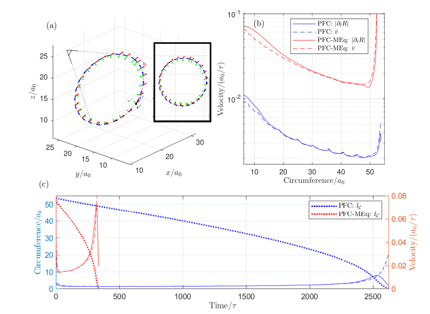
In order to obtain the velocity of the dislocation loop segments, we identify nodes on the loop and evaluate Eq. (16) by using numerical differentiation of the field to calculate the amplitude currents . To serve as a benchmark, we also calculate the circumference of the dislocation loop at each time (further details in A.5), so that we compare the rate of shrinkage
| (21) |
(solid blue line in Fig. 4(b)) to the average velocity of the dislocation nodes
| (22) |
(dashed blue line in Fig. 4(b)) where is the velocity of the dislocation line at node , calculated by the velocity formula Eq. (16). and should agree in the case of the shrinking of a perfectly circular loop and the figure shows excellent agreement between the two. Interestingly, we observe that both are sensitive to the Peierls like barriers during their motion, as shown by the oscillations in Fig. 4(b)). The maxima are separated by , confirming that the oscillation is related to the motion of a loop segment over one lattice spacing Boyer and Viñals 2002. This observation confirms that even though Eqs. (12) and (16) are continuum level descriptions of the system, they still exhibit behavior related to the underlying lattice configuration. The initial fast drop in velocity is due to the fast relaxation of the initial condition. The evolution of the variables under the dynamics of Eq. (18) are shown together with the evolution given by the PFC-MEq model which will be introduced in Sec. 3.3.
3.2 Theoretical analysis: Peach Koehler law
In this section, we show that the general expression Eq. (16) of the defect velocity agrees with the dissipative motion of a dislocation as given by the classical Peach-Koehler force Pismen 1999, Kosevich 1979. To calculate an analytical expression for the amplitude currents , we employ the amplitude formulation of the PFC model, which directly expresses the free energy and dynamical equations in terms of the complex amplitudes Goldenfeld et al. 2005, Athreya et al. 2006, Salvalaglio and Elder 2022. For our lattice symmetry, real valuedness of requires that , and the dynamical equations need only consider the amplitudes . By substituting Eq. (19) in and integrating over the unit cell, under the assumption of slowly-varying amplitudes, one obtains the following free energy as a function of the complex amplitudes,
| (23) |
where and . is a polynomial in and that depends in general on the specific crystalline symmetry under consideration Goldenfeld et al. 2005, Elder et al. 2010, Salvalaglio and Elder 2022 (here bcc, see E for its expression). Equation (23) is obtained when considering a set of vectors of length , while similar forms may be achieved when considering different length scales Elder et al. 2010, Salvalaglio et al. 2021. The evolution of , which follows from Eq. (18) is Goldenfeld et al. 2005, Salvalaglio and Elder 2022,
| (24) |
with
| (25) |
where the last term comes from the nonlinear contributions and in the local free energy density, and depend on the other amplitudes . However, for the amplitudes that go to zero at the defect, it can be shown that at the defect (for more details, see E). Thus, the evolution of near the defect core is dictated solely by the non-local gradient term, namely
| (26) |
Furthermore, this implies that the complex amplitude of a stationary defect satisfy at the core. We now add an imposed, smooth displacement to the amplitudes as to represent the far-field displacement induced by a different line segment, defect, or externally applied loads Skaugen et al. 2018a. This displacement is in addition to the discontinuous displacement field , described in Sec. 2, which is captured by stationary solution and defines the Burgers vector of the dislocation line (Fig. 2). Inserting this ansatz of the complex amplitudes into Eq. (11), and in the approximation of small distortions, , we find
| (27) |
where is the determinant vector field calculated from . The corresponding defect density current is
| (28) |
Arguably, the simplest solution of Eq. (26) is the isotropic, simple vortex which is linear with the distance from the core and . At a node on the dislocation line, can be written in terms of the Cartesian coordinates in the plane (Sec. 2), where it takes the form , with a proportionality constant. The gradients of can be evaluated in these coordinates and gives at , , from which we get the current
| (29) |
in terms of the local tangent vector . At , we also get , which leads to an expression of the dislocation velocity (where the proportionality constant cancels out), given by
| (30) |
where is the stress tensor for a bcc PFC that has been deformed by Skogvoll et al. 2021a,
| (31) |
Thus, the velocity of the dislocation line is proportional to the stress on the line. In vectorial form, this equation reads
| (32) |
with isotropic mobility .
A stationary dislocation induces a stress field , but only the imposed stress appears in the equation above. This is analogous to how the stress field of the dislocation itself is not included when the Peach-Koehler force as calculated Kosevich 1979. Thus, if is the configurational stress of the phase field at any given time, the part responsible for dislocation motion is the imposed stress
| (33) |
Note that the stationary solution necessarily satisfies mechanical equilibrium, , so that if the configurational PFC stress is in mechanical equilibrium, so is the imposed stress on the dislocation segment. The imposed stress used can be attributed to external load, other dislocations, or other parts of the dislocation loop. The framework predicts a defect mobility which is isotropic and does not discriminate between dislocation climb and glide motion. Numerically however, we have seen that at deeper quenches , climb motion is prohibited in the PFC model. The result in this section should therefore be interpreted as a first-order approximation, valid at shallow quenches. This apparent equal mobility for glide and climb may result from the employment of the amplitude phase-field model (which is only exact for ) or the assumption of an isotropic defect core in the calculation.
3.3 PFC dynamics constrained to mechanical equilibrium (PFC-MEq)
In the previous section, we found that the motion of a dislocation is governed by a configurational stress which derives from the PFC free energy. Since this stress is a functional only of the phase field configuration, it does not satisfy, in general, the condition of mechanical equilibrium. References Skaugen et al. 2018a, Skogvoll et al. 2021a give an explicit expression for this stress defined as the variation of the free energy with respect to distortion,
| (34) |
where is a spatial average over in order to eliminate the base periodicity of the phase field (see A.1).
In this section, we discuss a modification of the PFC in three dimensions and in an anisotropic lattice so as to maintain elastic equilibrium in the medium while evolves according to Eq. (18). Let be the field that results from the evolution defined by Eq. (18) alone. At each time, we define
| (35) |
where is a small continuous displacement computed so that the configurational stress associated with is divergence free. We now show a method to determine . Suppose that at some time the PFC configuration has an associated configurational stress (from Eq. (34), where ). Within linear elasticity, the stress after displacement of the current configuration by is given by
| (36) |
where is the elastic constant tensor, and . is determined by requiring that
| (37) |
By using the symmetry of the elastic constant tensor, we can rewrite this equation explicitly in terms of ,
| (38) |
where
| (39) |
is the body force from the stress Skogvoll et al. 2021a. The quantity is the free energy density from Eq. (17).
Given the periodic boundary conditions used, the system of equations (38) is solved by using a Fourier decomposition with the Green’s function for elastic displacement in cubic anisotropic materials Dederichs and Leibfried 1969. Once is obtained, is updated according to Eq. (35), and evolved according to Eq. (18) from its current state to . Note that Eqs. (38) can, in general, be solved for any elastic constant tensor, so that the method introduced is not limited to cubic anisotropy. Since the state can only be updated according to Eq. (35) every , this effectively sets a time scale of elastic relaxation in the model. We found that the numerical discretization scheme for imposing mechanical equilibrium at every has a slow convergence with decreasing time resolution. Thus, the rate of loop shrinkage also depends slightly on . This is further discussed in A.
Figure 4 contrasts numerical results for the evolution of an initial dislocation loop with and without using the method just described. The computed line velocities are very different as they are highly sensitive to the local stress experienced by the dislocation loop segments. This stems from the fact that under classical PFC dynamics, the stress is always given by , and a consequence of the results from Sec. 3.2 is that the velocity of an element of the defect line will be quite different depending on whether the stress acting on it is or . Figure 5 shows the dislocation loop after its circumference has shrunk to of its initial value, and the resulting component of the stress for both models.

As expected, the correction provided by the PFC-MEq model is necessary to relax the stress originating from the initial loop. The figure shows a large residual stress far from the dislocation loop that can only decay diffusively in the standard phase field model. Indeed, we have verified numerically that the configurational stress is only divergence-less for the PFC-MEq model. We note that in our set the loop is seeded in a glide plane, thus its shape remains approximately circular for both models, while the shrinkage rate is different. Note that with the addition of this advection step, the model is no longer guaranteed to be fully dissipative.
The problem addressed in this section involves finding the elastic distortion (which away from defects it can be written as for a displacement field ) given the dislocation density tensor as a state variable Acharya et al. 2019. The first part is the incompatibility of the elastic distortion
| (40) |
and the second is the mechanical equilibrium condition on
| (41) |
where is the tensor of elastic constants, and denotes the symmetric part of the tensor. Equation (40) has a non trivial kernel consisting of gradients of vector fields . This vector field is determined by Eq. (41) given appropriate boundary conditions that guarantee uniqueness. A computational method for solving for and , using the dislocation density as a state variable, was first given in Ref. Roy and Acharya 2005. The main difference between this reference and the method outlined in this section is that, since the incompatibility of the distortion is captured by the state of the phase field, we only need to solve for the compatible part of the distortion using the force density from the phase field as a source.
While the stress profile shown in Fig. 5(b), can be shown numerically to have vanishing divergence, we would like to see a direct comparison of the stress with the prediction from continuum elasticity. As the model purports to evolve the phase-field at mechanical equilibrium, and we are able to extract the dislocation density from the phase-field at any time through Eq. (12), this amounts to the problem of finding the stress tensor for a given dislocation density, under the constraint of mechanical equilibrium and with periodic boundary conditions (zero surface traction). This problem was adressed in Ref. Brenner et al. 2014, and in A.6, we show how we solve Equations (40-41) to derive the equilibrium stress field from using spectral methods. Figure 6 shows all the stress components after the dislocation loop has shrunk to of its initial diameter for both dynamical models, as well as the stress computed directly from the dislocation density tensor.11 1 Due to the geometric similarity in how the loop annihilates in the different models, there is no observable difference in the continuum elastic stress field predictions between using from either model as a source.

Note that the mean value of the components of , is not determined by Eqs. (40) - (41), and is set to zero. In this comparison, we have also subtracted from its mean value. As expected, the stresses obtained from the PFC-MEq model agree well with . The small differences observed are due to the fact that the configurational stress determined by is naturally regularized by the lattice spacing and the finite defect core, whereas the stress is for a continuum elastic medium with a singular dislocation source (numerically, the -functions in Eq. (12) is regularized by an arbitrary width of the Gaussian approximation). Investigating exactly which length scale of core regularization derives from the PFC model is an open and interesting question that we will address in the future.
4 Conclusions
We have introduced a theoretical method, and the associated numerical implementation, to study topological defect motion in a three dimensional, anisotropic, crystalline PFC lattice. The dislocation density tensor and velocity are directly defined by the spatially periodic phase field, where dislocations are identified with the zeros of its complex amplitudes.
To illustrate the method, we have studied the motion of a shear dislocation loop, and found that it accurately tracks the loop position, circumference, and velocity. As an application, we have shown that under certain simplifying assumptions, the overdamped dislocation velocity follows from the Peach-Koehler force, with the defect mobility determined by equilibrium lattice properties. We have introduced the PFC-MEq model for three dimensional anisotropic media which constrains the classical PFC model evolution to remain in mechanical equilibrium, and shown that loop motion is much faster with this modification. The PFC-MEq model produces stress profiles that are in agreement, especially far from the defect core, to stress fields directly computed from the instantaneous dislocation density tensor.
In summary, we have presented a comprehensive framework, based on the phase field crystal model for the analysis of dislocation motion in crystalline phases in three spatial dimensions. Starting from a free energy that has a ground state of the proper symmetry, the model naturally incorporates defects, the associated topological densities, and the resulting defect line kinematic laws that are compatible with topological density conservation. Configurational stresses induced by defects are defined and analyzed, and shown to lead to a Peach-Koehler type force on defects, with an explicit expression for the line segment mobility given.
Acknowledgements
V.S. and L.A. acknowledge support from the Research Council of Norway through the Center of Excellence funding scheme, Project No. 262644 (PoreLab). M.S. acknowledges support from the Emmy Noether Programme of the German Research Foundation (DFG) under Grant No. SA4032/2-1. The research of J.V. is supported by the National Science Foundation, contract No. DMR-1838977.
Appendix A Numerical methods
A.1 Amplitude demodulation
Given a phase-field configuration described by slowly varying amplitudes
| (42) |
we can find the amplitudes using the principle of resonance under coarse graining. Coarse graining with respect to a length scale is introduced as a convolution with a Gaussian filter function
| (43) |
Given the PFC configuration of Eq. (42), to find , we multiply by and coarse grain to get
| (44) |
where we have used the slowly varying nature of the complex amplitudes to pull them out of the coarse graining operation and used the resonance condition Skogvoll et al. 2021a.
A.2 Dislocation density tensor decomposition
A singular value decomposition of is introduced as , where is a diagonal matrix containing the singular values of , and and are unitary matrices containing the normalized eigenvectors of and , respectively. We assume that the dislocation density tensor can be written as the outer product of the unitary tangent vector and a local spatial Burgers vector density , i.e., . Under this assumption, one finds with only one non zero singular value, , and the columns of and that correspond to this singular value will be and , respectively.
A.3 Evolution of the phase field
The dimensionless parameters for the bcc ground state are set to: and . Lengths have been made dimensionless by choosing , yielding a bcc lattice constant . In all simulations, the computational domain is given by base periods of the undistorted bcc lattice, with grid spacing . Periodic boundary conditions are used throughout. Equation (18) is integrated forward in time with an explicit method Cox and Matthews 2002, and . A Fourier decomposition of the spatial fields is introduced to compute the spatial derivatives of the fields, while nonlinear terms are computed in real space.
A.3.1 Mechanical equilibrium
We implement the correction scheme of Eq. (35) between every timestep . If , we rescale so that , and repeat the process again until elastic equilibrium is achieved. Typically, when initializing the PFC field with a dislocation, around such iterations are needed, after which, is on the order of at each correction step.
The dislocation loop shrink velocity is sensitive to the time interval between each equilibration correction. As shown in Fig. 4, the effect of imposing this correction at every time interval accelerates the annihilation process by approximately a factor of . A slow convergence in the limit is observed, where we have estimated that the shrink velocity increases up to . However, to reach this numerical convergence is computationally demanding. Indeed, this slow convergence suggests that the time scale of the elastic field relaxation is important for the process of shear dislocation loop shrinkage. For static problems however, such as obtaining regularized stress profiles for dislocation loops, or defect nucleation under quasi-static loading, this slow convergence is not an issue.
A.4 Initializing a dislocation loop in the PFC model
In this section, we show how to multiply the initial amplitudes with complex phases, to produce a dislocation loop with Burgers vector in a slip plane given by normal vector (see Sec. 3.1). Given a point , it belongs to a plane perpendicular to for some point on the dislocation loop (see Figure 7).

This plane also intersects the diametrically opposed point of the dislocation loop. If is the center of the loop, the distance vector lies in . Let be the first and second coordinate in the Cartesian coordinate system defined by the right-handed orthonormal system centered at . If , we get from geometrical considerations
| (45) |
| (46) |
Both and are thus determined by , and the normal vector to the loop plane . () is the angle between () and in the plane and are found numerically by using the four-quadrant inverse tangent , so that
| (47) |
| (48) |
where is the radius of the loop. For each point , we determine and according to the equations above and initiate the PFC with the phases
| (49) |
where is given in Table 1.
| 1 | 0 | 0 | 0 | 1 | 1 | |
| 0 | 1 | 0 | 1 | 0 | -1 | |
| 0 | 0 | 1 | -1 | -1 | 0 | |
| 1 | 1 | 1 | 0 | 0 | 0 | |
| 0 | 1 | 1 | 0 | -1 | -1 | |
| 1 | 0 | 1 | -1 | 0 | 1 | |
| 1 | 1 | 0 | 1 | 1 | 0 |
This ensures that the complex phases have the right topological charge (Eq. (8)). The inset in Fig. 7 shows the phase of in for , which is the slip plane chosen in the simulation in Sec. 3.1. Note that points for which are computed by the same equation for the tangent vector at , with the same formula, thus validating the Eqs. (47)–(48) for all values in . Since the expressions are independent of the particular plane and each point belongs to one such plane, they are also valid for all points in the simulation domain.
A.5 Calculating the perimeter of a dislocation loop
To calculate numerically the perimeter of a dislocation loop, recall that
| (50) |
where we have added a subscript onto to emphasize that it is the point on the loop as indexed by the line element . Taking the double dot product with itself, we find
| (51) |
The contributions to this integral will only come from points on the loop and only when , where , so . Thus
| (52) |
Taking the square root and integrating over all space, we find
| (53) |
where is the perimeter of the dislocation loop. Thus,
| (54) |
A.6 Direct computation of stress fields
The dislocation density tensor is calculated directly from the phase field through Eq. (12). The general method of solving Eqs. (40-41) on a periodic medium is given in Ref. Brenner et al. 2014 given , where also the uniqueness of the elastic fields is proven given appropriate conditions on the dislocation density . In the present case, the conditions on are automatically satisfied as it is calculated from the phase-field. In this section, we thus show for our computational setup, how we compute the Green’s function in the relating the distortion to the dislocation density tensor as a source. Since (40-41) given the periodic boundary conditions can be solved uniquely, we Fourier transform both sets of equations and add the condition of mechanical equilibrium (Eq. (41)) to the diagonal equations () in Eq. (40), which gives in Fourier space
| (55) |
where there is no summation over , and we have multiplied the elastic constant tensor by where is the shear modulus of the cubic lattice, and . By defining the 1D vectors and as
we rewrite Eq. (55) more compactly as
| (56) |
where the explicit form of in the case of cubic anisotropy is given by
| (57) |
can be inverted to yield the Fourier transform of the distortion ,
| (58) |
Once (denoted by in components) is known, we compute the stress field in mechanical equilibrium
| (59) |
The dislocation density as obtained from the phase field as in Eq. (12) has a very small divergence due to numerical round-off errors. We impose explicitly before evaluating , which improves numerical stability.
Appendix B Inversion formula for highly symmetric lattice vector sets
In inverting Eq. (5) to obtain the displacement field in terms of the phases , we used the result of Eq. (6). This follows from the properties of moment tensors constructed from lattice vector sets . The -th order moment tensor constructed from is given by
| (60) |
In two dimensions, for a parity-invariant lattice vector set that has a B-fold symmetry, Ref. Chen and Orszag 2011 showed that all -th order moments vanish for odd and are isotropic for . Every isotropic rank 2 tensor is proportional to the identity tensor , so for a 2D lattice vector set having four-fold symmetry, such as the set of shortest reciprocal lattice vectors of the square lattice, we have (Figs. 3 and 5 in Ref. Skogvoll et al. 2021a show the reciprocal lattice vector sets discussed in this appendix). Taking the trace and using that the vectors have the same length , we get . In general, for any 2D parity invariant lattice vector set with a -fold symmetry where , we have
| (61) |
As mentioned, this holds for the 2D square lattice, but it also holds for the 2D hexagonal lattice. In fact, the six-fold symmetry of the hexagonal lattice ensures that also every fourth-order moment tensor is isotropic, which results in elastic properties of the 2D hexagonal PFC model being isotropic Skogvoll et al. 2021a.
To show this identity for a 3D parity invariant vector set with cubic symmetry, we generalize the proof in Ref. Chen and Orszag 2011 to a particular case of a 3D vector set that is symmetric with respect to rotations around each coordinate axis, such as the set of shortest reciprocal lattice vectors of bcc, fcc or simple cubic structures. Let be an eigenvector of with eigenvalue , i.e., . Since is invariant under a rotation around the -axis (i.e., ), we get , showing that is also an eigenvector of with the same eigenvalue . Repeating for a rotation around the -axis demonstrates that has only one eigenvalue , so that it must be proportional to the rank 2 identity tensor . Taking the trace and using that the vectors have the same length , we find
| (62) |
Appendix C Time derivatives of the dislocation density tensor
C.1 Delta-function form
Consider a moving dislocation line of points parametrized by the time and a dimensionless which can be taken to go from to without loss of generality. Keeping the labelling fixed through its time evolution, we get
| (63) |
Suppressing the dependence of on and , we get taking the time derivative of Eq. (2),
| (64) |
Starting with the first term using the chain rule, we have
| (65) |
where and is a field at time which is defined on as , the velocity of the line segment perpendicular to the tangent vector. We can rewrite and pull it outside the integral. Additionally, since is multiplied by a delta function, we can replace it by , so we get
| (66) |
Turning to the second term, we get
| (67) |
Since is multiplied with a delta-function inside the integral, we can replace it by . We thus get
| (68) |
since , either because is a loop such that or else since the dislocation cannot end inside the crystal. This gives
| (69) |
C.2 Amplitude form
Taking the time derivative of Eq. (12), we have
| (70) |
The vector field satisfies a conservation law which can be obtained by differentiating Eq. (11) with respect to time Angheluta et al. 2012, Mazenko 1999. This gives , with the associated current given by . Thus
| (71) |
Differentiating through the delta-function in the second term (2), we get
| (72) |
where and denotes the real and imaginary part of , respectively. Straight forward, but tedious algebra, shows that this is equal to
| (73) |
after inserting . Thus
| (74) |
Taken together, this gives
| (75) |
as desired.
Appendix D Calculation details of dislocation velocity
Inserting the expression for the delta-function in terms of the dislocation density tensor into Eq. (14), we get
| (76) |
Equating and at a point on the dislocation line, where using ,
| (77) |
We now integrate out the delta-function in the -plane and contract both sides of the equation with to get
| (78) |
as desired.
Appendix E Amplitude decoupling
The (complex) polynomial (see Eq. (23)) results from the amplitude expansion of the and terms in Eq. (17). It may be computed by substituting Eq. (19) into Eq. (17) and integrating over the unit cell, under the assumption of constant amplitudes Goldenfeld et al. 2005, Athreya et al. 2006, Salvalaglio and Elder 2022. It features terms reading , with and for which the condition is satisfied. By multiplying this condition by and using Eq. (8) it then follows that
| (79) |
In the equation for the dislocation velocity, Eq. (16), the only contributing amplitudes are those for which . The condition (79) implies that at least one of the other amplitudes, , appearing in terms of containing , also has and then vanishes at the corresponding defect. Thus, for a given amplitude with , the terms in always contain at least one vanishing amplitude. Eq. (25) then reduces to Eq. (26) at the defect as and there. Importantly, a full decoupling of the evolution equation for amplitudes which vanish at the defect is obtained.
This can be straightforwardly verified for specific lattice symmetries and dislocations. When accounting for the bcc lattice symmetry through as in Eq. (20), the (complex) polynomial entering the coarse-grained energy defined in Eq. (23) is
| (80) |
which gives
| (81) |
By comparing Eqs. (81) with the dislocation charges for the possible Burgers vector in the bcc lattice, Table 1, and noting that, at the dislocation core, for , we find
| (82) |
allowing for a decoupled system of evolution relations for , as described by Eq. (26).
References
- Acharya et al. [2019] A. Acharya, R. J. Knops, and J. Sivaloganathan. On the structure of linear dislocation field theory. Journal of the Mechanics and Physics of Solids, 130:216–244, September 2019. ISSN 0022-5096. doi: 10.1016/j.jmps.2019.06.002.
- Acharya and Viñals [2020] Amit Acharya and Jorge Viñals. Field dislocation mechanics and phase field crystal models. Physical Review B, 102(6):064109, August 2020. doi: 10.1103/PhysRevB.102.064109.
- Anderson et al. [2017] Peter M. Anderson, John P. Hirth, and Jens Lothe. Theory of Dislocations. Cambridge University Press, January 2017. ISBN 978-0-521-86436-7.
- Angheluta et al. [2012] Luiza Angheluta, Patricio Jeraldo, and Nigel Goldenfeld. Anisotropic velocity statistics of topological defects under shear flow. Phys. Rev. E, 85(1):011153, January 2012. doi: 10.1103/PhysRevE.85.011153.
- Archer et al. [2019] Andrew J. Archer, Daniel J. Ratliff, Alastair M. Rucklidge, and Priya Subramanian. Deriving phase field crystal theory from dynamical density functional theory: Consequences of the approximations. Physical Review E, 100(2):022140, August 2019. doi: 10.1103/PhysRevE.100.022140.
- Athreya et al. [2006] Badrinarayan P. Athreya, Nigel Goldenfeld, and Jonathan A. Dantzig. Renormalization-group theory for the phase-field crystal equation. Physical Review E, 74(1):011601, July 2006. doi: 10.1103/PhysRevE.74.011601.
- Berry et al. [2015] Joel Berry, Jörg Rottler, Chad W. Sinclair, and Nikolas Provatas. Atomistic study of diffusion-mediated plasticity and creep using phase field crystal methods. Phys. Rev. B, 92(13):134103, October 2015. doi: 10.1103/PhysRevB.92.134103.
- Boyer and Viñals [2002] Denis Boyer and Jorge Viñals. Weakly nonlinear theory of grain boundary motion in patterns with crystalline symmetry. Phys. Rev. Lett., 89(5):055501, 2002.
- Brazovskii [1975] S. Brazovskii. Phase transition of an isotropic system to a nonuniform state. Soviet Journal of Experimental and Theoretical Physics, 41:85, 1975.
- Brenner et al. [2014] R. Brenner, A.J. Beaudoin, P. Suquet, and A. Acharya. Numerical implementation of static Field Dislocation Mechanics theory for periodic media. Philosophical Magazine, 94(16):1764–1787, June 2014. ISSN 1478-6435. doi: 10.1080/14786435.2014.896081.
- Bulatov et al. [1998] Vasily Bulatov, Farid F. Abraham, Ladislas Kubin, Benoit Devincre, and Sidney Yip. Connecting atomistic and mesoscale simulations of crystal plasticity. Nature, 391(6668):669–672, February 1998. ISSN 1476-4687. doi: 10.1038/35577.
- Cai et al. [2006] Wei Cai, Athanasios Arsenlis, Christopher R. Weinberger, and Vasily V. Bulatov. A non-singular continuum theory of dislocations. Journal of the Mechanics and Physics of Solids, 54(3):561–587, March 2006. ISSN 0022-5096. doi: 10.1016/j.jmps.2005.09.005.
- Chen and Orszag [2011] Hudong Chen and Steven Orszag. Moment isotropy and discrete rotational symmetry of two-dimensional lattice vectors. Philosophical Transactions of the Royal Society A: Mathematical, Physical and Engineering Sciences, 369(1944):2176–2183, June 2011. doi: 10.1098/rsta.2010.0376.
- Cox and Matthews [2002] S. M. Cox and P. C. Matthews. Exponential Time Differencing for Stiff Systems. Journal of Computational Physics, 176(2):430–455, March 2002. ISSN 0021-9991. doi: 10.1006/jcph.2002.6995.
- Dederichs and Leibfried [1969] P. H. Dederichs and G. Leibfried. Elastic Green’s Function for Anisotropic Cubic Crystals. Physical Review, 188(3):1175–1183, December 1969. doi: 10.1103/PhysRev.188.1175.
- Devincre et al. [2008] B. Devincre, T. Hoc, and L. Kubin. Dislocation Mean Free Paths and Strain Hardening of Crystals. Science, 320(5884):1745–1748, June 2008. doi: 10.1126/science.1156101.
- Elder and Grant [2004] K. R. Elder and Martin Grant. Modeling elastic and plastic deformations in nonequilibrium processing using phase field crystals. Phys. Rev. E, 70(5):051605, November 2004. doi: 10.1103/PhysRevE.70.051605.
- Elder et al. [2002] K. R. Elder, Mark Katakowski, Mikko Haataja, and Martin Grant. Modeling Elasticity in Crystal Growth. Physical Review Letters, 88(24):245701, June 2002. doi: 10.1103/PhysRevLett.88.245701.
- Elder et al. [2007] K. R. Elder, Nikolas Provatas, Joel Berry, Peter Stefanovic, and Martin Grant. Phase-field crystal modeling and classical density functional theory of freezing. Physical Review B, 75(6):064107, February 2007. doi: 10.1103/PhysRevB.75.064107.
- Elder et al. [2010] K. R. Elder, Zhi-Feng Huang, and Nikolas Provatas. Amplitude expansion of the binary phase-field-crystal model. Phys. Rev. E, 81(1):011602, January 2010. doi: 10.1103/PhysRevE.81.011602.
- Emmerich et al. [2012] Heike Emmerich, Hartmut Löwen, Raphael Wittkowski, Thomas Gruhn, Gyula I. Tóth, György Tegze, and László Gránásy. Phase-field-crystal models for condensed matter dynamics on atomic length and diffusive time scales: An overview. Advances in Physics, 61(6):665–743, 2012. doi: 10.1080/00018732.2012.737555.
- Forster [1975] D. Forster. Hydrodynamic Fluctuations, Broken Symmetry, and Correlation Functions. Bejamin/Cummings, Reading, MA, 1975.
- Goldenfeld et al. [2005] Nigel Goldenfeld, Badrinarayan P. Athreya, and Jonathan A. Dantzig. Renormalization group approach to multiscale simulation of polycrystalline materials using the phase field crystal model. Phys. Rev. E, 72(2):020601, August 2005. doi: 10.1103/PhysRevE.72.020601.
- Halperin [1981] Bertrand I. Halperin. Statistical Mechanics of Topological Defects. In Roger Balian, Maurice Kléman, and Jean-Paul Poirier, editors, Physique Des Défauts/ Physics of Defects, pages 812–857. North-Holland, Amsterdam, 1981. ISBN 0-444-8622S-0.
- Heinonen et al. [2014] V. Heinonen, C. V. Achim, K. R. Elder, S. Buyukdagli, and T. Ala-Nissila. Phase-field-crystal models and mechanical equilibrium. Phys. Rev. E, 89(3):032411, March 2014. doi: 10.1103/PhysRevE.89.032411.
- Heinonen et al. [2016] V. Heinonen, C. V. Achim, J. M. Kosterlitz, See-Chen Ying, J. Lowengrub, and T. Ala-Nissila. Consistent Hydrodynamics for Phase Field Crystals. Physical Review Letters, 116(2):024303, January 2016. doi: 10.1103/PhysRevLett.116.024303.
- Hill [1998] Rodney Hill. The Mathematical Theory of Plasticity. Clarendon Press, 1998. ISBN 978-0-19-850367-5.
- Huang et al. [2010] Zhi-Feng Huang, K. R. Elder, and Nikolas Provatas. Phase-field-crystal dynamics for binary systems: Derivation from dynamical density functional theory, amplitude equation formalism, and applications to alloy heterostructures. Physical Review E, 82(2):021605, August 2010. doi: 10.1103/PhysRevE.82.021605.
- Kosevich [1979] A. M. Kosevich. Crystal dislocations and the theory of elasticity. In F. R. N. Nabarro, editor, Dislocations in Solids, Vol. 1, pages 33–141. North-Holland, Amsterdam, 1979.
- Koslowski et al. [2002] M. Koslowski, A. M. Cuitiño, and M. Ortiz. A phase-field theory of dislocation dynamics, strain hardening and hysteresis in ductile single crystals. Journal of the Mechanics and Physics of Solids, 50(12):2597–2635, December 2002. ISSN 0022-5096. doi: 10.1016/S0022-5096(02)00037-6.
- Kubin et al. [1992] Ladislas P. Kubin, G. Canova, M. Condat, Benoit Devincre, V. Pontikis, and Yves Bréchet. Dislocation microstructures and plastic flow: A 3D simulation. In Non Linear Phenomena in Materials Science II, volume 23 of Solid State Phenomena, pages 455–472. Trans Tech Publications Ltd, January 1992. doi: 10.4028/www.scientific.net/SSP.23-24.455.
- Lazar [2014] Markus Lazar. On gradient field theories: Gradient magnetostatics and gradient elasticity. Philosophical Magazine, 94(25):2840–2874, September 2014. ISSN 1478-6435. doi: 10.1080/14786435.2014.935512.
- Lazar [2017] Markus Lazar. Non-singular dislocation continuum theories: Strain gradient elasticity vs. Peierls–Nabarro model. Philosophical Magazine, 97(34):3246–3275, December 2017. ISSN 1478-6435. doi: 10.1080/14786435.2017.1375608.
- Lazar and Maugin [2005] Markus Lazar and Gérard A. Maugin. Nonsingular stress and strain fields of dislocations and disclinations in first strain gradient elasticity. International Journal of Engineering Science, 43(13):1157–1184, September 2005. ISSN 0020-7225. doi: 10.1016/j.ijengsci.2005.01.006.
- Liu et al. [2020] Zhe-Yuan Liu, Ying-Jun Gao, Qian-Qian Deng, Yi-Xuan Li, Zong-Ji Huang, Kun Liao, and Zhi-Rong Luo. A nanoscale study of nucleation and propagation of Zener types cracks at dislocations: Phase field crystal model. Computational Materials Science, 179:109640, June 2020. ISSN 0927-0256. doi: 10.1016/j.commatsci.2020.109640.
- Mazenko [1997] Gene F. Mazenko. Vortex velocities in the O(n) symmetric time-dependent ginzburg-landau model. Phys. Rev. Lett., 78(3):401–404, January 1997. doi: 10.1103/PhysRevLett.78.401.
- Mazenko [1999] Gene F. Mazenko. Velocity distribution for strings in phase-ordering kinetics. Physical Review E, 59(2):1574–1584, February 1999. doi: 10.1103/PhysRevE.59.1574.
- Mianroodi and Svendsen [2015] Jaber Rezaei Mianroodi and Bob Svendsen. Atomistically determined phase-field modeling of dislocation dissociation, stacking fault formation, dislocation slip, and reactions in fcc systems. Journal of the Mechanics and Physics of Solids, 77:109–122, April 2015. ISSN 0022-5096. doi: 10.1016/j.jmps.2015.01.007.
- Momeni et al. [2018] Kasra Momeni, Yanzhou Ji, Kehao Zhang, Joshua A. Robinson, and Long-Qing Chen. Multiscale framework for simulation-guided growth of 2D materials. npj 2D Materials and Applications, 2(1):1–7, September 2018. ISSN 2397-7132. doi: 10.1038/s41699-018-0072-4.
- Pismen [1999] Len Pismen. Vortices in nonlinear fields: from liquid crystals to superfluids, from non-equilibrium patterns to cosmic strings, volume 100. Oxford University Press, 1999.
- Pokharel et al. [2014] Reeju Pokharel, Jonathan Lind, Anand K. Kanjarla, Ricardo A. Lebensohn, Shiu Fai Li, Peter Kenesei, Robert M. Suter, and Anthony D. Rollett. Polycrystal Plasticity: Comparison Between Grain - Scale Observations of Deformation and Simulations. Annual Review of Condensed Matter Physics, 5(1):317–346, 2014. doi: 10.1146/annurev-conmatphys-031113-133846.
- Provatas et al. [2007] N. Provatas, J. A. Dantzig, B. Athreya, P. Chan, P. Stefanovic, N. Goldenfeld, and K. R. Elder. Using the phase-field crystal method in the multi-scale modeling of microstructure evolution. JOM, 59(7):83–90, July 2007. ISSN 1543-1851. doi: 10.1007/s11837-007-0095-3.
- Ramos et al. [2010] J. A. P. Ramos, E. Granato, S. C. Ying, C. V. Achim, K. R. Elder, and T. Ala-Nissila. Dynamical transitions and sliding friction of the phase-field-crystal model with pinning. Phys. Rev. E, 81(1):011121, January 2010. doi: 10.1103/PhysRevE.81.011121.
- Rodney et al. [2003] D. Rodney, Y. Le Bouar, and A. Finel. Phase field methods and dislocations. Acta Materialia, 51(1):17–30, January 2003. ISSN 1359-6454. doi: 10.1016/S1359-6454(01)00379-2.
- Rollett et al. [2015] A. D. Rollett, G. S. Rohrer, and R. M. Suter. Understanding materials microstructure and behavior at the mesoscale. MRS Bulletin, 40(11):951–960, November 2015. ISSN 0883-7694, 1938-1425. doi: 10.1557/mrs.2015.262.
- Roters et al. [2010] F. Roters, P. Eisenlohr, L. Hantcherli, D. D. Tjahjanto, T. R. Bieler, and D. Raabe. Overview of constitutive laws, kinematics, homogenization and multiscale methods in crystal plasticity finite-element modeling: Theory, experiments, applications. Acta Materialia, 58(4):1152–1211, February 2010. ISSN 1359-6454. doi: 10.1016/j.actamat.2009.10.058.
- Roy and Acharya [2005] Anish Roy and Amit Acharya. Finite element approximation of field dislocation mechanics. Journal of the Mechanics and Physics of Solids, 53(1):143–170, January 2005. ISSN 0022-5096. doi: 10.1016/j.jmps.2004.05.007.
- Salvalaglio and Elder [2022] Marco Salvalaglio and Ken R Elder. Coarse-grained modeling of crystals by the amplitude expansion of the phase-field crystal model: an overview. Modelling and Simulation in Materials Science and Engineering, 2022. doi: 10.1088/1361-651X/ac681e.
- Salvalaglio et al. [2018] Marco Salvalaglio, Rainer Backofen, K. R. Elder, and Axel Voigt. Defects at grain boundaries: A coarse-grained, three-dimensional description by the amplitude expansion of the phase-field crystal model. Physical Review Materials, 2(5):053804, May 2018. doi: 10.1103/PhysRevMaterials.2.053804.
- Salvalaglio et al. [2019] Marco Salvalaglio, Axel Voigt, and Ken R. Elder. Closing the gap between atomic-scale lattice deformations and continuum elasticity. npj Computational Materials, 5(1):48, 2019. ISSN 2057-3960. doi: 10.1038/s41524-019-0185-0.
- Salvalaglio et al. [2020] Marco Salvalaglio, Luiza Angheluta, Zhi-Feng Huang, Axel Voigt, Ken R. Elder, and Jorge Viñals. A coarse-grained phase-field crystal model of plastic motion. Journal of the Mechanics and Physics of Solids, 137:103856, 2020. ISSN 0022-5096. doi: 10.1016/j.jmps.2019.103856.
- Salvalaglio et al. [2021] Marco Salvalaglio, Axel Voigt, Zhi-Feng Huang, and Ken R. Elder. Mesoscale Defect Motion in Binary Systems: Effects of Compositional Strain and Cottrell Atmospheres. Physical Review Letters, 126(18):185502, May 2021. doi: 10.1103/PhysRevLett.126.185502.
- Sills et al. [2016] Ryan B. Sills, William P. Kuykendall, Amin Aghaei, and Wei Cai. Fundamentals of Dislocation Dynamics Simulations. In Christopher R. Weinberger and Garritt J. Tucker, editors, Multiscale Materials Modeling for Nanomechanics, Springer Series in Materials Science, pages 53–87. Springer International Publishing, Cham, 2016. ISBN 978-3-319-33480-6. doi: 10.1007/978-3-319-33480-6_2.
- Skaugen et al. [2018a] Audun Skaugen, Luiza Angheluta, and Jorge Viñals. Dislocation dynamics and crystal plasticity in the phase-field crystal model. Phys. Rev. B, 97(5):054113, February 2018a. doi: 10.1103/PhysRevB.97.054113.
- Skaugen et al. [2018b] Audun Skaugen, Luiza Angheluta, and Jorge Viñals. Separation of elastic and plastic timescales in a phase field crystal model. Phys. Rev. Lett., 121(25):255501, December 2018b. doi: 10.1103/PhysRevLett.121.255501.
- Skogvoll et al. [2021a] Vidar Skogvoll, Audun Skaugen, and Luiza Angheluta. Stress in ordered systems: Ginzburg-Landau-type density field theory. Physical Review B, 103(22):224107, June 2021a. doi: 10.1103/PhysRevB.103.224107.
- Skogvoll et al. [2021b] Vidar Skogvoll, Audun Skaugen, Luiza Angheluta, and Jorge Viñals. Dislocation nucleation in the phase-field crystal model. Physical Review B, 103(1):014107, January 2021b. doi: 10.1103/PhysRevB.103.014107.
- Stefanovic et al. [2006] Peter Stefanovic, Mikko Haataja, and Nikolas Provatas. Phase-field crystals with elastic interactions. Phys. Rev. Lett., 96(22):225504, June 2006. doi: 10.1103/PhysRevLett.96.225504.
- Swift and Hohenberg [1977] J. Swift and P. C. Hohenberg. Hydrodynamic fluctuations at the convective instability. Physical Review A, 15(1):319–328, January 1977. doi: 10.1103/PhysRevA.15.319.
- Tóth et al. [2013] Gyula I. Tóth, László Gránásy, and György Tegze. Nonlinear hydrodynamic theory of crystallization. Journal of Physics: Condensed Matter, 26(5):055001, December 2013. ISSN 0953-8984. doi: 10.1088/0953-8984/26/5/055001.
- Wu [2004] Han-Chin Wu. Continuum Mechanics and Plasticity. Chapman and Hall/CRC, New York, December 2004. ISBN 978-0-429-20880-5. doi: 10.1201/9780203491997.
- Wu and Voorhees [2012] Kuo-An Wu and Peter W. Voorhees. Phase field crystal simulations of nanocrystalline grain growth in two dimensions. Acta Materialia, 60(1):407–419, January 2012. ISSN 1359-6454. doi: 10.1016/j.actamat.2011.09.035.
- Yamanaka et al. [2017] Akinori Yamanaka, Kevin McReynolds, and Peter W. Voorhees. Phase field crystal simulation of grain boundary motion, grain rotation and dislocation reactions in a BCC bicrystal. Acta Materialia, 133:160–171, July 2017. ISSN 1359-6454. doi: 10.1016/j.actamat.2017.05.022.