Dynamical Friction From Ultralight Dark Matter
Abstract
We simulate the gravitational dynamics of a massive object interacting with Ultralight / Fuzzy Dark Matter (ULDM/FDM), non-relativistic quantum matter described by the Schrödinger-Poisson equation. We first consider a point mass moving in a uniform background, and then a supermassive black hole (SMBH) moving within a ULDM soliton. After replicating simple dynamical friction scenarios to verify our numerical strategies, we demonstrate that the wake induced by a moving mass in a uniform medium may undergo gravitational collapse that dramatically increases the drag force, albeit in a scenario unlikely to be encountered astrophysically. We broadly confirm simple estimates of dynamical friction timescales for a black hole at the center of a halo but see that a large moving point mass excites coherent “breathing modes” in a ULDM soliton. These can lead to “stone skipping” trajectories for point masses which do not sink uniformly toward the center of the soliton, as well as stochastic motion near the center itself. These effects will add complexity to SMBH-ULDM interactions and to SMBH mergers in a ULDM universe.
I Introduction
We analyse a point-like massive particle interacting with self-gravitating quantum matter. The overall investigation is motivated by the dynamics of super-massive black holes (SMBH) moving inside Ultralight Dark Matter (ULDM) halos. ULDM, also known as Fuzzy Dark Matter, is based on non-interacting particles with de Broglie wavelengths long enough to influence galactic dynamics on sub-kiloparsec scales (Preskill et al. 1983; Abbott and Sikivie 1983; Dine and Fischler 1983; Turner 1983; Khlopov et al. 1985; Press et al. 1990; Hu et al. 2000; Sin 1994; Sahni and Wang 2000; Matos et al. 2000; Guzmán and Matos 2000; Goodman 2000; Peebles 2000; Amendola and Barbieri 2006; Hwang and Noh 2009; Marsh 2016; Niemeyer 2020). Common realisations of this scenario are built on axions with masses in the range eV. ULDM is non-relativistic quantum matter interacting with its own Newtonian gravitational potential and is thus governed by the nonlinear Schrödinger-Poisson equation.
On large scales, ULDM resembles cold dark matter (CDM) but its quantum properties become apparent on smaller scales, modifying the expectations for intra-galactic dynamics relative to CDM Hui et al. 2017. Given that conventional CDM faces a number of challenges when confronted with the small-scale properties of galaxies, these differences are the primary motivation for ULDM models, and understanding the detailed dynamics of ULDM will be key to testing these scenarios. Moreover, in addition to ULDM, self-gravitating quantum matter may arise in the very early universe Musoke et al. 2020; Eggemeier et al. 2021, hypothetical boson stars Guzmán and Ureña López 2004; Schwabe et al. 2016; Mocz et al. 2017 and QCD axion miniclusters Eggemeier and Niemeyer 2019, so the underlying dynamical system is relevant to wide range of astrophysical systems.
This work is complementary to that of Lancaster et al. Lancaster et al. 2020 who give numerical and analytic treatments of both point-like and extended masses moving through a ULDM background. We provide more numerical detail, but focus on point masses. The uniform background case is primarily a test for our code, recovering known analytic solutions (which are analogous to a much older problem in electron propagation (Landau and Lifshitz 1977)) in the limit where the self-gravity of the quantum matter is ignored and the point mass moves with constant velocity. However, a point mass moving in an otherwise undisturbed ULDM background leaves an elongated overdensity in its wake, which eventually undergoes gravitational collapse. The deep potential of the resulting overdensity then brings the moving mass to a rapid standstill.
Conversely, when a black hole interacts with a ULDM halo the central soliton has already collapsed and is supported by “quantum pressure”. We consider a the idealized scenario of a mass in an initially circular orbit around an unperturbed soliton. We broadly confirm simple estimates of the timescales over which an orbiting mass sinks to the center of the halo. However, the moving mass excites oscillations in the soliton independently of the dynamical friction, and the resulting motion can be complicated and stochastic. In particular, we see possible evidence that an orbiting black hole will be “reheated” as it interacts with the now-dynamical soliton for some parameter combinations. This appears to increase the likelihood of core-stalling in SMBH mergers in a ULDM dominated universe in a way that is distinct from the heating of black hole binaries by the granular nature of ULDM halos, described by Bar-Or et al. Bar-Or et al. 2018. Consequently,for both uniform backgrounds and solitonic configurations we find that non-perturbative backreaction introduces qualitatively new phenomena into ULDM dynamics.
This work rests on numerical solutions of the coupled Schrödinger-Poisson equation. Our simulations are based on PyUltraLight Edwards et al. 2018a, a pseudo-spectral Schrödinger-Poisson solver written in Python (with the FFTs provided by compiled libraries) which has been modified to include point mass ensembles that react to the gravitational potential of the combined ULDM-matter system.11 1 The code can be found at https://github.com/Sifyrena/PyUL_NBody.
Astrophysical constraints on the axion mass paint a complex picture Marsh and Hoof 2021. Lyman- forest data has been used to establish eV at 95% confidence Rogers and Peiris 2021. Studies of Eridanis-II Marsh and Niemeyer 2019 rule out the range eV, although any given system may be far from equilibrium when observed Kendall and Easther 2020a, complicating both “single object” constraints and treatments using idealized ULDM profiles Bar et al. 2021. Conversely, superradiance Stott and Marsh 2018 excludes masses eV but these bounds would soften in the presence of even weak self-interactions. Separately, recent large scale structure constraints Hlozek et al. 2015 imply that eV Dentler et al. 2021. In what follows we set the axion mass to eV for the idealised scenario of a point mass moving in a uniform ULDM background. This system has no direct astrophysical analogue and could be treated dimensionlessly. However, this value is often adopted as a fiducial ULDM mass (Ferreira 2020) and providing concrete numbers contextualizes the results. When looking at interactions between point masses and ULDM solitons we set eV, given that larger values are broadly preferred by the data although our overall focus here is the underlying dynamics of these systems, not their detailed astrophysics.
This paper is arranged as follows. In Section II, we outline the Schrödinger-Poisson equation and approximate analytical treatments of dynamical friction. We describe the numerical implementation of this system in Section III, validating the code against known results. In Section IV we present the results for a heavy object moving in a ULDM background and the resulting gravitational collapse of the wake and we examine black hole-soliton interactions in Section V.
II Background
II.1 The Framework of ULDM Dynamics
In non-relativistic limit, our system is governed by
| (1a) | ||||
| (1b) | ||||
where is the ULDM wavefunction, and is the axion mass. The gravitational potential due to the ULDM wavefunction is while is the gravitational potential sourced by the N body particles, which themselves evolve via
| (2a) | ||||
| (2b) | ||||
Equations 1a and 1b constitute the Schrödinger-Poisson equation with an external, time-varying potential.
Idealized ULDM halos contain a central soliton which is the ground state solution of the Schrödinger-Poisson equation (Schive et al. 2014; Kendall and Easther 2020b). Soliton density profiles may be obtained to arbitrary numerical precision by imposing spherical symmetry on , or
| (3) |
where and is a constant whose value is to be numerically determined. If we define , equations 1a and 1b reduce to
| (4) | ||||
| (5) |
in the time-independent limit, where is the radial derivative. The relevant boundary conditions are , , and at a large enough cut-off radius , which ensures that the profile is smooth at the origin.
If is a solution to the spherically symmetric Schrödinger-Poisson equation, then
| (6) |
where is an arbitrary scaling constant, is also a solution. It is thus straight-forward to restore physical units and initialize a 3D simulation by making appropriate choices of .
II.2 Steady State Gravitational Wakes
As a massive object travels through a diffuse medium some of its kinetic energy and momentum may be injected into the medium. This effective drag force is known as dynamical friction. These interactions can be purely gravitational: the “wake” behind a moving object is over-dense and gives rise to a force on the object opposed to its direction of motion.
Following the approach pioneered by Chandrasekhar (Chandrasekhar 1943) it is common and usually sufficient to ignore the subsequent evolution of the medium driven by its gravitational self-interaction. In this limit and with a constant velocity for the point mass ULDM dynamics can be viewed as Coulomb scattering (Landau and Lifshitz 1977; Hui et al. 2017) by working in the frame in which a stationary mass is subject to an “axion wind”. Consequently, we assume the particle of mass is at the origin immersed in an axion flow with velocity and density when undisturbed.
Ignoring axion self-gravity and denoting the radial coordinate , the system obeys the time-independent Schrödinger equation ,
| (7) |
This has an analytical solution in the form of a confluent hypergeometric function,
| (8) |
In Equation II.2, is the axion de Broglie wavelength and the inverse quantum Mach number is
| (9) |
and we have
| (10) |
where is the Pochhammer symbol,
| (11) |
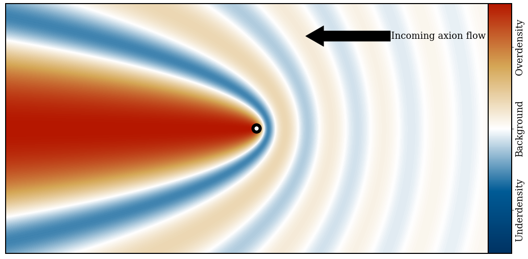
Figure 1 illustrates a typical density profile.
The dynamical friction is supplied by the gravitational field of the over-dense wake. However, a naive integral of the source over diverges since the overdensity approaches a non-zero constant value at arbitrary large distances behind the moving mass. This problem (which stems from the unphysical assumption that the semi-infinite wake can be generated at a constant velocity within finite time) is solved by introducing a spatial cutoff scale, , the distance traveled by the mass relative to the medium. It is also helpful to expresses in units of the axion de Broglie wavelength, denoted as ,
| (12) |
If the mass travels at constant velocity, the dynamical friction is (Hui et al. 2017; Lancaster et al. 2020)
| (13) |
where is a friction coefficient. The gravitational force on the mass is , so approximately we have
| (14) |
When we can extract from the wavefunction, Equation 7,
| (15) |
where and . In the limit that , one evaluates
| (16) |
III Numerical Methodology

III.1 Units and Scales
The program mass, time, and length units (, , and respectively) are as follows:
| (17a) | ||||
| (17b) | ||||
| (17c) | ||||
where is the present Hubble constant, is the matter fraction, and .
III.2 ULDM Dynamics
For a domain of edge length and resolution , the simulation mesh grid involves a set of points:
| (18) |
where , , and are integers between and .
To advance Equations 1a and 1b, we approximate the unitary time evolution of the quantum field using the symmetrized split-step Fourier method, applied from right to left:
| (19) |
where () denotes the (inverse) discrete Fourier transform on the grid. The ULDM gravitational potential is obtained by solving Poisson equation in the frequency domain,
| (20) |
This method is correct to second order in time Edwards et al. 2018b.
III.3 Time-step and Boundary Conditions
The ULDM velocity is manifest as the gradient in the phase of ; phase differences greater than radians are associated with numerical breakdown and a “strobing” effect that can lead to structure appearing to move in the wrong direction. By default, the integration step length, , is chosen using the Courant–Friedrichs–Lewy (CFL) condition, such that an object with the highest speed resolvable by the grid travels exactly one grid interval during one time step, or
| (21) |
The CFL condition is a qualitative requirement in this context, given that the Schrödinger-Poisson equation is not a hyperbolic system (Edwards et al. 2018a), but it provides a useful starting point and we have tested our results for sensitivity to the specific choice of timestep. The N body integrator takes 32 Runge-Kutta 4 (RK4) integration steps during the time .
Our simulation has periodic spatial boundary conditions. For the case of a black hole moving in a uniform ULDM background we limit the duration of simulations to
| (22) |
so that the ULDM wake is prevented from “wrapping round” the periodic boundary. This is less of an issue when the black hole interacts with a soliton.
III.4 N Body Dynamics
Particle potentials are implemented as Plummer spheres (Plummer 1911) to suppress numerical irregularities at grid crossings22 2 Note that this model does not capture short-range strong-field gravitational phenomena, such as superradiance. A particle with mass at location has a gravitational potential
| (23) |
where , and is the Plummer radius; for small this approximates an ideal point mass.
Fourier series obtained for and from the pseudospectral algorithm (Equations III.2 and 20) are only guaranteed to converge to the solution at the spatial grid points; evaluating them at arbitrary positions induces spurious sub-grid structure in . Consequently, we advance Equation 2b by estimating using a trilinear interpolation which makes use of values at the particle’s nearest grid points. The algorithm is shown schematically in Figure 2.
IV Dynamical Friction in a Uniform ULDM Medium
IV.1 A Model Without Self-Gravity

We begin with simulations without ULDM self-gravity. As before, we assume a mass moving along the axis in an initially uniform ULDM medium at a constant velocity. Unless noted otherwise, the simulations shown in this section are produced with:
These quantities can be calibrated against expectations for the central solitonic condensations of ULDM halos (Schive et al. 2014):
| (24a) | ||||
| (24b) | ||||
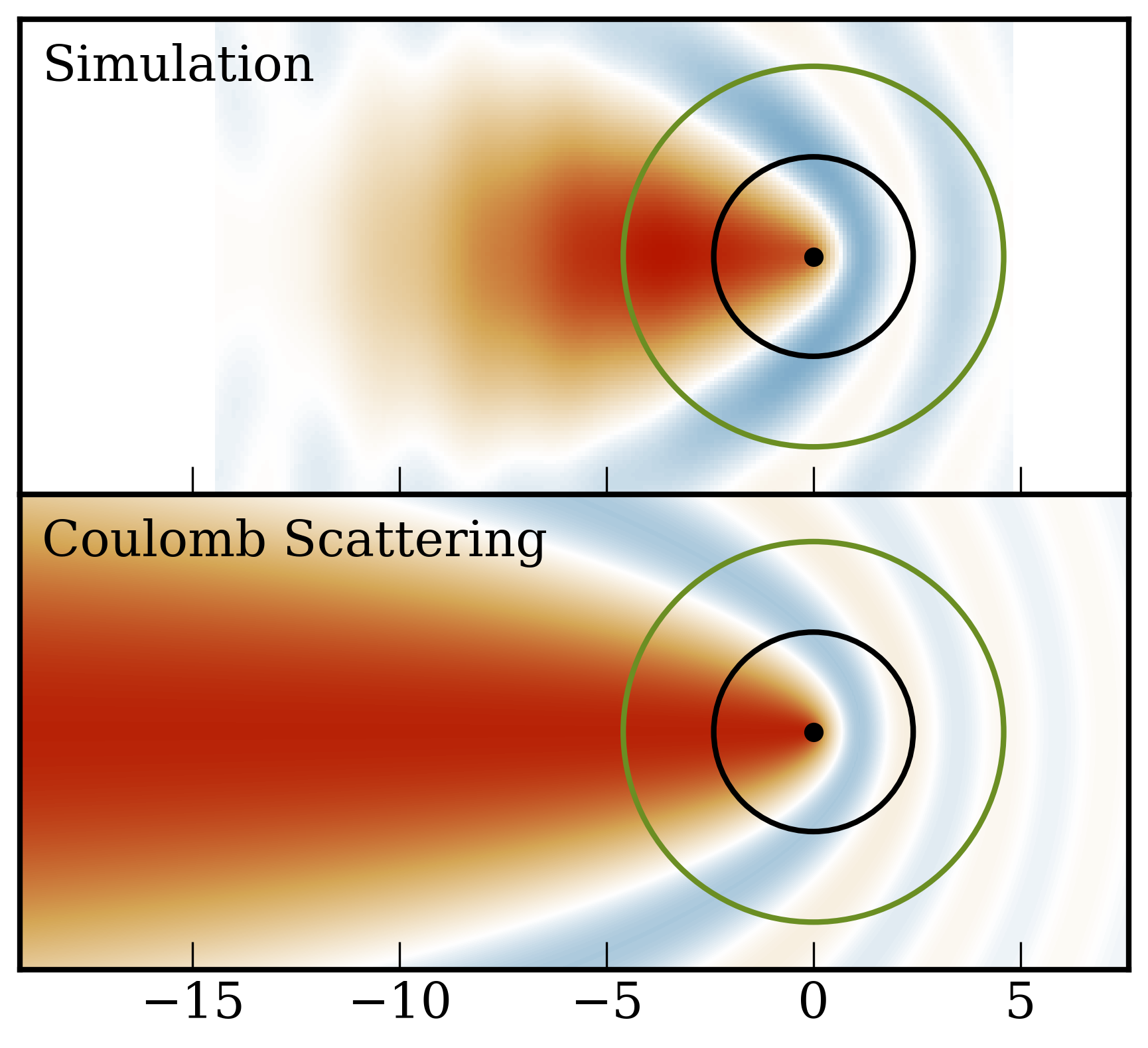
where and are the central density and HWHM radius of a halo with virialized mass . The background density in our simulations is similar to that of the solitonic core of a halo, but our uniform-density simulated volume is substantially larger than the soliton. In Figure 3 we compare a simulation (with axion self-gravity disabled) to the steady state Coulomb solution. There is good qualitative overlap between the two solutions in the the vicinity of the mass point. However, the wake is truncated in the numerical simulation as a consequence of the finite duration of the calculation.

We can work with two inertial frames, the ULDM frame and the initially comoving frame. In the former, the mass has initial velocity in a stationary ULDM background. In the latter, the mass is initially at rest, embedded in a ULDM background moving with velocity . Figure 4 illustrates that our simulations are consistent between these frames.

If the dynamical friction does not alter significantly, Equation 12 reduces to
| (25) |
Evaluating via Equation 15, we can quantitatively compare the simulation with the analytical results, as shown in Figure 5. The simulation results are obtained via Equation 14, which is a direct measure of the force. This is a nontrivial result, in that it demonstrates that using a “cutoff” to compute the dynamical friction is a good match to that given by the time-dependent wake.
IV.2 Simulations with Self-Gravity


We now enable ULDM self-gravity and allow the traveling mass to slow down in response to the ULDM potential. In this case, the wake undergoes gravitational collapse forming a high-density region behind the particle. The resulting gravitational potential greatly increases the dynamical friction, bringing the particle to a rapid halt.
Figure 6 illustrates the time-evolution of such an overdensity. It initially tracks the previous case, but eventually tips over into a runaway collapse. We plot and for our representative solution in Figure 7. Once the collapse is well underway, decreases, causing to similarly decrease.
In Figure 8, we show the energy transfer between the moving mass and the background medium in the two reference frames. In the initially comoving frame the total kinetic energy is larger since a much greater mass of ULDM is moving toward the black hole, in contrast to the ULDM rest frame in which only the black hole is moving initially. In both cases we find good energy conservation, but the total amount of energy is not invariant under the Galilean transformation. In the lower plot we see that energy conservation improves with resolution as we would expect. Conservation appears to be better in comoving frame. However, this is a byproduct of the axion flow carrying more kinetic energy than the moving mass, rather than a physical distinction.
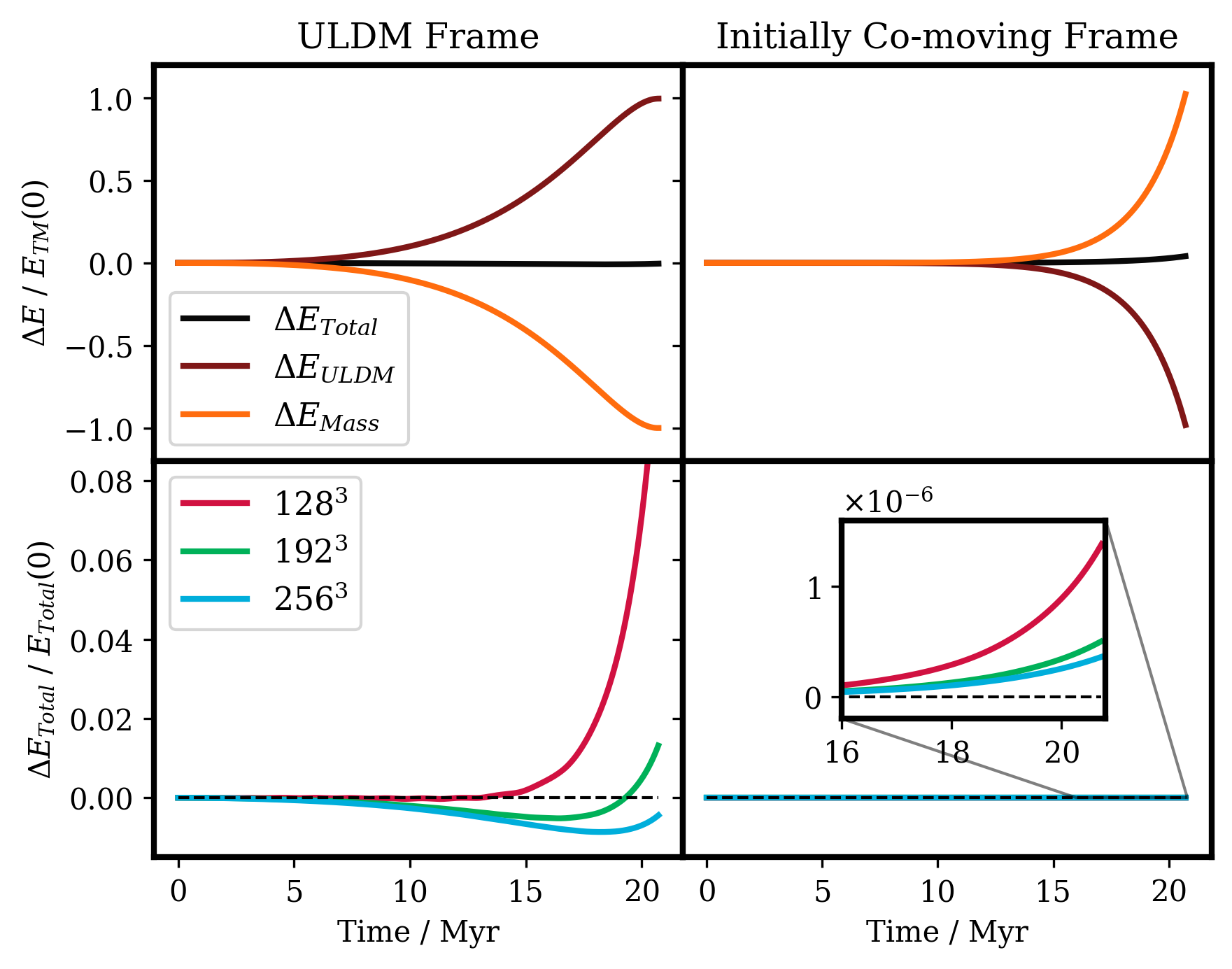
Figure 9 shows the dependence on mesh resolution and the Plummer radius. We see that decreasing the Plummer radius increases the friction and decreases stopping distance, as expected Lancaster et al. 2020. We also verify a sub-grid Plummer radius can be chosen without inducing numerical instability. Conversely, if we fix the Plummer radius relative to the grid spacing, decreasing effectively makes the potential more diffuse, so stopping time increases as is reduced. However, one can extrapolate to the continuum limit without difficulty.


When the self-gravity term in the Schrödinger-Poisson equation is small the Coulomb scattering approximation is typically sufficient to compute the force on a moving particle. However, once the wake becomes gravitationally unstable the particle rapidly slows down. To illustrate this we surveyed a range of initial particle masses between and million solar masses and ULDM densities between and . In almost all cases the moving mass came to halt after traveling less than 3.5 kpc and within 100 Myr. For large black holes in a very dense ULDM background the stopping distance can be on the order of parsecs.


Physically, however, this scenario is unlikely to be encountered in practice - the densest parts of a ULDM are the central soliton, which need not behave in the same way as a uniform ULDM background. Conceivably conditions close to this scenario could exist in the early universe (recalling that at recombination) but in that scenario the moving object would necessarily be a primordial black hole, formed in a much earlier epoch. Moreover, in this scenario axion collapse may lead to the formation of a black hole, as studied in Ref. (Helfer et al. 2017).
V ULDM Solitons
V.1 Physical Configuration
We now consider a mass moving in an initially circular orbit around (and inside) a Schrödinger-Poisson soliton and analyze the decay of its orbital radius and energy. SMBH dynamics after a galactic merger are obviously a key motivation for this work but we focus on a single, displaced SMBH in this initial treatment.
The simulations in this Section make use of a soliton with the parameters
where is the radius which encloses of the soliton mass.33 3 These numbers cannot all be chosen independently; any two of them fully specify the properties of the soliton. The chosen axion mass ( eV) is broadly compatible with current astrophysical bounds (although see Rogers and Peiris 2021); the mass of the central soliton is consistent with that expected for a halo Schive et al. 2014; Hui et al. 2017. The simulations are performed in a box kpc on a side and the Plummer radius is set to be half of the grid-spacing.
Our simulations begin with the black hole embedded in an undisturbed soliton. Figure 11 shows the ULDM configuration at four different times for a mass ratio of . There is no obvious wake, since the ULDM background responds to both quantum pressure, and its own confining gravitational potential, but the overall soliton is disturbed by the passage of the black hole.
Figure 12 shows the trajectories of two black holes (from separate simulations) with masses and in initially circular orbits; the more massive black hole feels a larger dynamical friction and quickly sinks towards the center. The center of mass is at the origin, so the more massive black hole has a smaller initial radial position.

V.2 Numerical Considerations
These simulations are performed in PyUltraLight with periodic boundary conditions; to suppress artifacts arising from interactions with the boundary the simulation volume is necessarily much larger than the soliton. However, our results are largely insensitive to the spatial resolution of the ULDM simulation and energy conservation scales as expected with resolution, as shown in Figure 13.
The resolution-independence of these simulations is perhaps surprising, given that the whole trajectory in Figure 13 fits into a region only a few mesh grids across for . However, this welcome result makes physical sense given that dynamical friction arises from a collective interaction between the black hole and the overall soliton, in contrast to drag forces associated with the mechanical displacement of a medium which are thus largely local phenomena. Consequently, provided the soliton is adequately resolved our simulations quickly reach a resolution-independent limit as is increased. Recall too that the black hole position varies continuously with the lattice on which the wavefunction is obtained. With , lattice points are about 11pc apart, which is on the order of the minimum radial separation attained after the black hole has sunk toward the center of the soliton.
V.3 Dynamical Friction
Figure 14 shows the trajectories for five black hole masses and two different starting radii. The black holes all initially sink toward the center but their kinetic energies need not decrease monotonically, due to their interactions with the newly disturbed soliton.
For circular motion the dynamical friction applies a torque on the moving mass, which gives the rate of change in the angular momentum. This implicitly defines a (rough) timescale for the orbital lifetime (Hui et al. 2017)
| (26) |
where is the initial orbital angular momentum and is the ULDM mass inside the radius . We invoke Equation 16 to write
| (27) |
which yields
| (28) |
where we have explicitly denoted the density is function of . Hui et al. (Hui et al. 2017) assume that the black hole is near the center of the soliton and replace with its maximum value; after this substitution it is immediately clear that as .


For a particle with mass orbiting this specific soliton at the resulting timescale is
| (29) |
recalling that is 8% of the soliton mass, the largest ratio we consider. Figure 15 plots the characteristic timescale for a range of masses and radii, rescaled by . As noted above, diverges at small , since the circular velocity decreases at the center of a spherical mass distribution, and likewise at large when the density of the medium and and velocity both decrease with radius, but it is roughly constant for intermediate radii.
The derivation of the timescale in Equation 28 implicitly assumes a linear and steady decrease in angular momentum but the simulated black hole orbital radii are clearly non-monotonic. We obtain an empirical timescale for comparison purposes from the interval over which the black hole angular momentum with respect to origin decreases by 20%44 4 In the simulations with the smallest black holes starting from the largest radii this threshold is never actually reached; for these cases we extrapolate., and then rescale to the obtain the projected time to reach .
There is reasonable agreement between our dynamical estimates and the computed value of , given that it is, at best, an indicative value rather than a detailed prediction. Consequently, these results can be seen as a numerical verification of the semi-analytic treatments of the dynamical friction experienced by point masses interacting with ULDM solitons, even through the classical wakes seen in the previous Section do not form in these systems.
V.4 Soliton Backreaction

In principle, the approximation in Equation 28 could be improved by integrating the instantaneous torque to yield the time taken to move between any two given radii. This would be less valuable in practice, given that in many cases the orbits are far from circular. For our chosen configuration, the black hole faces a force opposed to its initial velocity causing it to “fall” toward the center, accelerating as it does so, as illustrated in Figure 16. More massive black holes follow a clearly spiral trajectory toward the center, as seen in Figure 12, and can undergo effectively stochastic motion upon their arrival in the central region of the soliton. This motion is reminicent of the “reheating” experienced by a massive particle when it is introduced to the centers of an already excited soliton (Dutta Chowdhury et al. 2021).


The individual components of the total energy for a simulation with pc and are shown in Figure 17. The overall energy of the black hole decreases as it sinks towards the center of the soliton. However, we also see the onset of a persistent oscillation in the soliton itself, even though its total energy is constant, outside of the energy injected by the moving black hole. This is attributable to our chosen initial configuration which puts a stationary, spherically symmetric soliton in the potential of an adjacent black hole. This is a small perturbation to the overall gravitational potential of the soliton, but it means that it is no longer in its ground state configuration. The soliton is also relatively “compressible” – the overall change in its self-potential is several times larger than the potential energy of the black hole. T he impact of the breathing mode on the potential is illustrated in Figure 19, which shows the trajectories of black holes for a series of different starting radii.
Physically, this is a breathing mode, albeit one likely to break spherical symmetry given the off-center position of the external gravitational field. The oscillations persist on timescales much longer than those over which the black hole orbit decays as there is no mechanism to remove this energy from the system. Moreover, they persist even if the black hole is deleted from the simulation after it has completed a number of orbits.

Beyond the stochastic motion seen at the center of the soliton, for certain parameter choices the breathing mode “reheats” black holes orbiting at some distance from the center. This is illustrated in Figure 19, which shows a set of trajectories in which the radial distance of the black hole steadily increases over a number of orbits. Physically, this behavior appears to be driven by a resonance between the soliton breathing mode and the orbital period; a similar situation is described in Ref. (Annulli et al. 2020). It is more pronounced for small black holes (since it has to work against the dynamical friction, which increases with mass) and depends non-linearly on the initial radius, which fixes the specific form of the breathing mode. This behavior (which is reminiscent of a stone skipped across a pond) is responsible for much of the scatter seen in Figure 15.
VI Conclusion and Discussions
We have presented simulations of (large) point masses interacting with ultralight dark matter (ULDM), and focused on two scenarios – a uniform background of ULDM and the soliton found at the center of a ULDM galactic halo. In the former, the wake left by the moving point mass can collapse under its self-gravity, dramatically enhancing the dynamical friction. We then simulate the dynamics of a super-massive black hole in an initially circular orbit about (and inside of) a ULDM soliton. The black hole sinks towards the center of the soliton. We confirm simple estimates of the relevant timescale within but also see novel “stone skipping” trajectories at certain large initial radii, where the black hole does not monotonically approach the center. Once near the center, black holes undergo stochastic motion, migrating back out to radii of 10s of parsecs in the examples we study. Both the stone skipping and the stochastic trajectories are driven by excitations to the soliton sourced by its interactions with black hole.
Astrophysically, there may be few circumstances in which a point mass will encounter a uniform and otherwise unperturbed background, although one can imagine possible scenarios involving primordial black holes or very early universe physics Musoke et al. 2020; Eggemeier et al. 2021. Conversely, a massive object inside a Schrödinger-Poisson soliton maps directly to the dynamics of SMBH at the center of a galactic halo, and these systems have a wide range of astrophysical consequences. Identifying the ways in which the distinctive properties of ULDM modify our expectations for these interactions could be key to testing the scenario, given the potential of pulsar timing experiments Burke-Spolaor et al. 2019 and the upcoming LISA mission Amaro-Seoane et al. 2017.
This investigation focused on a single black hole interacting with an initially unperturbed soliton but the interactions between two (or more) SMBH in a single, post-merger halo are of particular interest. These systems are fascinating in their own right, given that most large galaxies at low-redshifts have a single central SMBH but are likely to be the products of mergers in the evolving universe. Consequently, it appears that the merger dynamics of SMBH must, to some extent, recapitulate the merger trees of their host galaxies. However, the actual processes that bring SMBH close enough to ensure that gravitational wave emission drives mergers on timescales less than the present age of the Universe are poorly understood. Consequently, determining whether ULDM can solve – or exacerbate – this so-called “final parsec problem” Milosavljevic and Merritt 2003; Barausse and Lapi 2020 is a promising strategy for testing the overall scenario. Applying the tools developed here to the dynamics of multiple SMBH interacting within ULDM solitons is an obvious extension of this work.
The present results complement suggestions by Bar-Or et al. Bar-Or et al. 2018 that black hole binaries will be “heated” by interactions with a granular ULDM halo. In the present case the ULDM is initially uniform and large scale oscillations are induced as the soliton-SMBH system orbits its common center of mass. In a post-merger halo, the central soliton may be far from its ground state, suggesting that these effects might be substantially enhanced in astrophysical settings, resulting in the outward diffusion of light objects residing in the center of the soliton (Dutta Chowdhury et al. 2021). In addition, the coupling and impulsive heating associated with a single SMBH-soliton interaction could be analyzed in detail using eigenstate expansions of the soliton potential Zagorac et al. 2021, facilitating the semi-analytic treatment of these systems.
Perhaps surprisingly it seems that the interactions between ULDM solitons and the black hole motion are well-modeled even at low grid resolutions. This rather fortunate outcome arises from the difficulty of establishing large density gradients in ULDM on scales significantly shorter than the de Broglie wavelength; the black hole effectively interacts with the overall soliton, rather than just the matter in its immediate locality. That said, there is clear value in high-resolution simulations. However, we are obliged to simulate a large volume to prevent the soliton from being disrupted by boundary effects so the black hole trajectory is confined to a small fraction of the total simulation region. Consequently, implementing the combination of a hard -body solver coupled to a Schrödinger-Poisson solver in a scheme that supports adaptive mesh refinement (e.g. Ref. Schwabe et al. 2020) is a logical next step.
We see interesting interactions at larger radii driven by “breathing modes” of the soliton excited by its interaction with the black hole. In these cases black holes at relatively large distances do not sink monotonically toward the center of the soliton. These “stone skipping” trajectories differ from previous work on the dynamical friction in ULDM (e.g. Lancaster et al. 2020; Bar-Or et al. 2018 in that they represent interactions between the point mass and the overall soliton, and point to further novel behaviors associated with SMBH-ULDM dynamics.
The breathing modes driving the stone skipping solutions are reminiscent of quasinormal modes arising from displacements of a Schrödinger-Poisson system away from its equilibrium configuration (Guzmán and Ureña López 2004; Zagorac et al. 2021). These analyses can presumably be generalized to the asymmetric states seen here, allowing a more quantitative understanding of these trajectories.
In summary, this work explores the dynamical friction acting on a massive point particle traversing through self-gravitating quantum matter, and investigates interactions between black holes and Schrödinger-Poisson solitons. This creates a pathway toward the detailed study of these systems in contexts ranging from boson stars, ultralight dark matter, to the early universe.
Acknowledgements.
We thank Katy Clough, Mateja Gosenca, Lilian Guo, Peter Hayman, Shaun Hotchkiss, Emily Kendall, Priyamvada Natarajan, Jens Niemeyer, Nikhil Padmanabhan, and Luna Zagorac for useful discussions. We acknowledge support from the Marsden Fund of the Royal Society of New Zealand. The simulations in this paper were performed on the Australian National eResearch Collaboration Tools and Resources (NeCTAR) platform, hosted at the University of Auckland. The authors acknowledge the use of New Zealand eScience Infrastructure (NeSI) high performance computing facilities and consulting support as part of this research.References
- Preskill et al. (1983) J. Preskill, M. B. Wise, and F. Wilczek, Phys. Lett. B 120, 127 (1983).
- Abbott and Sikivie (1983) L. Abbott and P. Sikivie, Phys. Lett. B 120, 133 (1983).
- Dine and Fischler (1983) M. Dine and W. Fischler, Phys. Lett. B 120, 137 (1983).
- Turner (1983) M. S. Turner, Phys. Rev. D 28, 1243 (1983).
- Khlopov et al. (1985) M. I. Khlopov, B. A. Malomed, and I. B. Zeldovich, Mon. Not. R. Astron. Soc. 215, 575 (1985).
- Press et al. (1990) W. H. Press, B. S. Ryden, and D. N. Spergel, Phys. Rev. Lett. 64, 1084 (1990).
- Hu et al. (2000) W. Hu, R. Barkana, and A. Gruzinov, Phys. Rev. Lett.s 85, 1158 (2000).
- Sin (1994) S.-J. Sin, Phys. Rev. D 50, 3650 (1994).
- Sahni and Wang (2000) V. Sahni and L. Wang, Phys. Rev. D 62, 103517 (2000), arXiv:astro-ph/9910097 [astro-ph] .
- Matos et al. (2000) T. Matos, F. S. Guzmán, and L. A. Ureña-López, Classical and Quantum Gravity 17, 1707 (2000), arXiv:astro-ph/9908152 [astro-ph] .
- Guzmán and Matos (2000) F. S. Guzmán and T. Matos, Classical and Quantum Gravity 17, L9 (2000), arXiv:gr-qc/9810028 [gr-qc] .
- Goodman (2000) J. Goodman, New Astronomy 5, 103 (2000).
- Peebles (2000) P. J. E. Peebles, The Astrophysical Journal 534, L127 (2000).
- Amendola and Barbieri (2006) L. Amendola and R. Barbieri, Physics Letters B 642, 192 (2006).
- Hwang and Noh (2009) J.-C. Hwang and H. Noh, Physics Letters B 680, 1 (2009), arXiv:0902.4738 [astro-ph.CO] .
- Marsh (2016) D. J. E. Marsh, Physics Reports 643, 1 (2016).
- Niemeyer (2020) J. C. Niemeyer, Progress in Particle and Nuclear Physics 113, 103787 (2020).
- Hui et al. (2017) L. Hui, J. P. Ostriker, S. Tremaine, and E. Witten, Phys. Rev. D 95 (2017), 10.1103/PhysRevD.95.043541, arXiv:1610.08297 .
- Musoke et al. (2020) N. Musoke, S. Hotchkiss, and R. Easther, Phys. Rev. Lett. 124, 061301 (2020), arXiv:1909.11678 [astro-ph.CO] .
- Eggemeier et al. (2021) B. Eggemeier, J. C. Niemeyer, and R. Easther, Phys. Rev. D 103, 063525 (2021), arXiv:2011.13333 [astro-ph.CO] .
- Guzmán and Ureña López (2004) F. S. Guzmán and L. A. Ureña López, Phys. Rev. D 69, 124033 (2004).
- Schwabe et al. (2016) B. Schwabe, J. C. Niemeyer, and J. F. Engels, Phys. Rev. D 94, 043513 (2016).
- Mocz et al. (2017) P. Mocz, M. Vogelsberger, V. H. Robles, J. Zavala, M. Boylan-Kolchin, A. Fialkov, and L. Hernquist, Monthly Notices of the Royal Astronomical Society 471, 4559 (2017).
- Eggemeier and Niemeyer (2019) B. Eggemeier and J. C. Niemeyer, Phys. Rev. D 100, 063528 (2019).
- Lancaster et al. (2020) L. Lancaster, C. Giovanetti, P. Mocz, Y. Kahn, M. Lisanti, and D. N. Spergel, JCAP 01, 001 (2020), arXiv:1909.06381 [astro-ph.CO] .
- Landau and Lifshitz (1977) L. D. Landau and E. M. Lifshitz, Course of theoretical physics III: Quantum mechanics, Non-relativistic theory (3rd ed.) (1977).
- Bar-Or et al. (2018) B. Bar-Or, J. B. Fouvry, and S. Tremaine, arXiv (2018), 10.3847/1538-4357/aaf28c, arXiv:1809.07673 .
- Edwards et al. (2018a) F. Edwards, E. Kendall, S. Hotchkiss, and R. Easther, J. Cosmol. Astropart. Phys. 2018 (2018a), 10.1088/1475-7516/2018/10/027, arXiv:1807.04037 .
- Marsh and Hoof (2021) D. J. E. Marsh and S. Hoof, (2021), arXiv:2106.08797 [hep-ph] .
- Rogers and Peiris (2021) K. K. Rogers and H. V. Peiris, Phys. Rev. Lett. 126, 071302 (2021), arXiv:2007.12705 [astro-ph.CO] .
- Marsh and Niemeyer (2019) D. J. E. Marsh and J. C. Niemeyer, Phys. Rev. Lett. 123, 051103 (2019), arXiv:1810.08543 [astro-ph.CO] .
- Kendall and Easther (2020a) E. Kendall and R. Easther, Publ. Astron. Soc. Austral. 37, e009 (2020a), arXiv:1908.02508 [astro-ph.CO] .
- Bar et al. (2021) N. Bar, K. Blum, and C. Sun, (2021), arXiv:2111.03070 [hep-ph] .
- Stott and Marsh (2018) M. J. Stott and D. J. E. Marsh, Phys. Rev. D 98, 083006 (2018), arXiv:1805.02016 [hep-ph] .
- Hlozek et al. (2015) R. Hlozek, D. Grin, D. J. E. Marsh, and P. G. Ferreira, Phys. Rev. D 91, 103512 (2015), arXiv:1410.2896 [astro-ph.CO] .
- Dentler et al. (2021) M. Dentler, D. J. E. Marsh, R. Hložek, A. Laguë, K. K. Rogers, and D. Grin, (2021), arXiv:2111.01199 [astro-ph.CO] .
- Ferreira (2020) E. G. M. Ferreira, (2020), arXiv:2005.03254 .
- Schive et al. (2014) H.-Y. Schive, T. Chiueh, and T. Broadhurst, Nature Physics 10, 496 (2014), arXiv:1406.6586 .
- Kendall and Easther (2020b) E. Kendall and R. Easther, Publ. Astron. Soc. Aust. (2020b), 10.1017/pasa.2020.3, arXiv:1908.02508 .
- Chandrasekhar (1943) S. Chandrasekhar, Astrophys. J. 97, 255 (1943).
- Edwards et al. (2018b) F. Edwards, E. Kendall, S. Hotchkiss, and R. Easther, JCAP 10, 027 (2018b), arXiv:1807.04037 [astro-ph.CO] .
- Plummer (1911) H. C. Plummer, Mon. Not. R. Astron. Soc. 71, 460 (1911).
- Schive et al. (2014) H.-Y. Schive, M.-H. Liao, T.-P. Woo, S.-K. Wong, T. Chiueh, T. Broadhurst, and W.-Y. P. Hwang, Phys. Rev. Lett. 113, 261302 (2014).
- Helfer et al. (2017) T. Helfer, D. J. Marsh, K. Clough, M. Fairbairn, E. A. Lim, and R. Becerril, Journal of Cosmology and Astroparticle Physics 2017, 055–055 (2017).
- Dutta Chowdhury et al. (2021) D. Dutta Chowdhury, F. C. van den Bosch, V. H. Robles, P. van Dokkum, H.-Y. Schive, T. Chiueh, and T. Broadhurst, The Astrophysical Journal 916, 27 (2021).
- Annulli et al. (2020) L. Annulli, V. Cardoso, and R. Vicente, Phys. Rev. D 102, 063022 (2020), arXiv:2009.00012 [gr-qc] .
- Burke-Spolaor et al. (2019) S. Burke-Spolaor et al., Astron. Astrophys. Rev. 27, 5 (2019), arXiv:1811.08826 [astro-ph.HE] .
- Amaro-Seoane et al. (2017) P. Amaro-Seoane et al. (LISA), (2017), arXiv:1702.00786 [astro-ph.IM] .
- Milosavljevic and Merritt (2003) M. Milosavljevic and D. Merritt, Astrophys. J. 596, 860 (2003), arXiv:astro-ph/0212459 .
- Barausse and Lapi (2020) E. Barausse and A. Lapi, (2020), arXiv:2011.01994 [astro-ph.GA] .
- Zagorac et al. (2021) J. L. Zagorac, I. Sands, N. Padmanabhan, and R. Easther, (2021), arXiv:2109.01920 [astro-ph.CO] .
- Schwabe et al. (2020) B. Schwabe, M. Gosenca, C. Behrens, J. C. Niemeyer, and R. Easther, Phys. Rev. D. , 1 (2020), arXiv:2007.08256 .