Mandal et al \righttitleNatural Language Engineering
Article
100 \jnlDoiYr2019 \doival10.1017/xxxxx
(Received xx xxx xxx; revised xx xxx xxx; accepted xx xxx xxx)
Is Attention always needed? A Case Study on Language Identification from Speech
Abstract
Language Identification (LID) is a crucial preliminary process in the field of Automatic Speech Recognition (ASR) that involves the identification of a spoken language from audio samples. Contemporary systems that can process speech in multiple languages require users to expressly designate one or more languages prior to utilization. The LID task assumes a significant role in scenarios where ASR systems are unable to comprehend the spoken language in multilingual settings, leading to unsuccessful speech recognition outcomes. The present study introduces convolutional recurrent neural network (CRNN) based LID, designed to operate on the Mel-frequency Cepstral Coefficient (MFCC) characteristics of audio samples. Furthermore, we replicate certain state-of-the-art methodologies, specifically the Convolutional Neural Network (CNN) and Attention-based Convolutional Recurrent Neural Network (CRNN with attention), and conduct a comparative analysis with our CRNN-based approach. We conducted comprehensive evaluations on thirteen distinct Indian languages and our model resulted in over 98% classification accuracy. The LID model exhibits high-performance levels ranging from 97% to 100% for languages that are linguistically similar. The proposed LID model exhibits a high degree of extensibility to additional languages and demonstrates a strong resistance to noise, achieving 91.2% accuracy in a noisy setting when applied to a European Language (EU) dataset.
1 Introduction
In the era of the Internet of Things, smart and intelligent assistants (e.g., Alexa 11 1 https://developer.amazon.com/en-US/alexa/alexa-voice-service; Siri 22 2 https://www.apple.com/in/siri/; Cortana 33 3 https://www.microsoft.com/en-in/windows/cortana; Google Assistant 44 4 https://assistant.google.com/; etc.) can interact with humans with some default language settings (mostly in English) and these smart assistants rely heavily on ASR. The motivation for our work stems from the inadequacy of virtual assistants in providing support in multilingual settings. In order to enhance the durability of intelligent assistants, LID can be implemented to enable automatic recognition of the speaker’s language, thereby facilitating appropriate language setting adjustments. Psychological behaviour exhibits that Humans have an inherent capability to determine the language of a statement nearly instantly. Automatic LID seeks to classify a speaker’s language usage from their speech utterances.
We focus our study of LID on Indian Languages since India is the world’s second most populated and seventh largest country in landmass and a linguistically diverse country. Currently, India has 28 states and 8 Union Territories, where each state and Union Territories has its own language, but none of the languages is recognised as the national language of the country. Only, English and Hindi are used as official languages according to the Constitution of India Part XVII Chapter 1 Article 34355 5 https://www.mea.gov.in/Images/pdf1/Part17.pdf. Currently, the Eighth Schedule of the Constitution consists of 22 languages. Table 1 describes the recognised 22 languages according to the Eighth Schedule of the Constitution of India, as of 1 December 2007.
| Sl. No. | Language | Family | Spoken in | |||||
|---|---|---|---|---|---|---|---|---|
| 1 | Assamese | Indo-Aryan | Assam | |||||
| 2 | Bengali | Indo-Aryan | Assam, Jharkhand, Tripura, West Bengal | |||||
| 3 | Bodo | Sino-Tibetan | Assam | |||||
| 4 | Dogri | Indo-Aryan | Jammu & Kashmir | |||||
| 5 | Gujarati | Indo-Aryan | Gujrat, Dadra & Nagar Haveli & Daman & Diu | |||||
| 6 | Hindi | Indo-Aryan |
| |||||
| 7 | Kannada | Dravidian | Karnataka | |||||
| 8 | Kashmiri | Indo-Aryan | Jammu & Kashmir | |||||
| 9 | Konkani | Indo-Aryan | Dadra & Nagar Haveli & Daman & Diu, Goa | |||||
| 10 | Maithili | Indo-Aryan | Jharkhand | |||||
| 11 | Malayalam | Dravidian | Kerala, Lakshadweep, Puducherry | |||||
| 12 | Manipuri | Sino-Tibetan | Manipur | |||||
| 13 | Marathi | Indo-Aryan |
| |||||
| 14 | Nepali | Indo-Aryan | Sikkim, West Bengal | |||||
| 15 | Odia | Indo-Aryan | Jharkhand, Odisha | |||||
| 16 | Punjabi | Indo-Aryan | Delhi, Haryana, Punjab | |||||
| 17 | Sanskrit | Indo-Aryan | Himachal Pradesh | |||||
| 18 | Santali | Austroasiatic | Jharkhand | |||||
| 19 | Sindhi | Indo-Aryan | Rajasthan | |||||
| 20 | Tamil | Dravidian | Tamil Nadu | |||||
| 21 | Telugu | Dravidian | Andhra Pradesh, Puducherry, Telangana | |||||
| 22 | Urdu | Indo-Aryan |
|
Most of the Indian languages originated from the Indo-Aryan and Dravidian language families. It can be seen from Table 1 that different languages are spoken in different states, however, languages do not obey geographical boundaries. Therefore, many of these languages, particularly in the neighbouring regions, have multiple dialects which are amalgamations of two or more languages.
Such enormous linguistic diversity makes it difficult for citizens to communicate in different parts of the country. Bilingualism and multilingualism are the norms in India. In this context, a LID system becomes a crucial component for any speech-based smart assistant. The biggest challenge and hence an area of active innovation for the Indian language is the reality that most of these languages are under-resourced.
Every spoken language has its underlying lexical, speaker, channel, environment, and other variations. The likely differences among various spoken languages are in their phoneme inventories, frequency of occurrence of the phonemes, acoustics, the span of the sound units in different languages, and intonation patterns at higher levels. The overlap between the phoneme set of two or more familial languages makes it a challenge for recognition. The low-resource status of these languages makes the training of machine learning models doubly difficult. The idea behind our methodology is interesting on account of the aforementioned limitations. Our methodology involves forecasting the accurate spoken language, irrespective of the limitations mentioned earlier.
CNN has been heavily utilized by Natural Language Processing (NLP) researchers from the very beginning due to their efficient use of local features. While Recurrent Neural Networks (RNNs) have been shown to be effective in a variety of NLP tasks in the past, recent work with Attention-based methods have outperformed all previous models and architectures because of their ability to capture global interactions. Yamada et al, 2020 were able to achieve better results than BERT (Devlin et al, 2019), SpanBERT (Joshi et al, 2020), XLNet (Yang et al, 2019), and ALBERT (Zhenzong et al, 2020) using their Attention-based methods in the Question-Answering domain. Researchers (Takase et al, 2021; Gu et al, 2019; Chen et al, 2020) have employed Attention-based methods to achieve state-of-the-art (SOTA) performance in Machine Translation. Transformers (Vaswani et al, 2017), which utilize a self-attention mechanism, have found extensive application in almost all fields of NLP such as language modelling, text classification, topic modelling, emotion classification, sentiment analysis, etc., and produced SOTA performance.
In this work, we present LID for Indian languages using a combination of CNN, RNN, and Attention-based methods. Our LID methods cover 13 Indian languages66 6 The study was limited to the number of Indian languages for which datasets were available. Additionally, our method is language agnostic. The main contributions of this work can be summarized as follows:
- •
We carried out exhaustive experiments using CNN, CRNN, and attention-based CRNN for the LID task on 13 Indian languages and achieved state-of-the-art results.
- •
The model exhibits exceptional performance in languages that are part of the same language family, as well as in diverse language sets under both normal and noisy conditions.
- •
We empirically proved that CRNN framework achieves better or similar results compared to CRNN with Attention framework although CRNN without Attention requires less computational overhead.
2 Related Works
Extraction of language-dependent features for example prosody and phonemes was widely used to classify spoken languages (Zissman, 1996; Martinez et al, 2020; Ferrer et al, 2010). Following the success of speaker verification systems, identity vectors (i-vectors) have also been used as features in various classification frameworks. Use of i-vectors requires significant domain knowledge (Dehak et al, 2011; Martinez et al, 2020). In recent trends, researchers rely on neural networks for feature extraction and classification (Lopez-Moreno et al, 2014; Ganapathy et al, 2014). Researcher Revay and Teschke, 2019 used the ResNet50 (He et al, 2016) framework for classifying languages by generating the log-Mel spectra for each raw audio. The framework uses a cyclic learning rate where the learning rate increases and then decreases linearly. The maximum learning rate for a cycle is set by finding the optimal learning rate using fastai (Howard et al, 2020).
Researcher Gazeau et al, 2018 established the use of a Neural Network, Support Vector Machine, and Hidden Markov Model (HMM) to identify different languages. Hidden Markov models convert speech into a sequence of vectors and are used to capture temporal features in speech. Established LID systems (Dehak et al, 2011; Martinez et al, 2020; Plchot et al, 2016; Zazo et al, 2016) are based on identity vector (i-vectors) representations for language processing tasks. In Dehak et al, 2011, i-vectors are used as data representations for a speaker verification task and fed to the classifier as the input. Dehak et al, 2011 applied Support Vector Machines (SVM) with cosine kernels as the classifier, while Martinez et al, 2020 used logistic regression for the actual classification task. Recent years have found the use of feature extraction with neural networks, particularly with Long Short Term Memory (LSTM) (Zazo et al, 2016; Gelly et al, 2016; Lozano-Diez et al, 2015). These neural networks produce better accuracy while being simpler in design compared to the conventional LID methods (Dehak et al, 2011; Martinez et al, 2020; Plchot et al, 2016). Recent trends in developing LID systems are mainly focused on different forms of LSTMs with DNNs. Plchot et al, 2016 used a 3-layered CNN where i-vectors were the input layer and softmax activation function was the output layer. Zazo et al, 2016 used MFCC with Shifted Delta Coefficient features as information to a unidirectional layer that is directly connected to a softmax classifier. Gelly et al, 2016 used audio transformed to Perceptual Linear Prediction (PLP) coefficients and their and order derivatives as information for a Bidirectional LSTM in forward and backward directions. The forward and backward sequences generated from the Bidirectional LSTM were joined together and used to classify the language of the input samples. Lozano-Diez et al, 2015 used CNNs for their LID system. They transformed the input data into an image containing MFCCs with Shifted Delta Coefficient features. The image represents the time domain for the x-axis and frequency bins for the y-axis.
Lozano-Diez et al, 2015 used CNN as the feature extractor for the identity vectors. They achieved better performance when combining both the CNN features and identity vectors. Revay and Teschke, 2019 used ResNet (He et al, 2016) framework for language classification by generating spectrograms of each audio. Cyclic Learning (Smith, 2018) was used where the learning rate increases and decreases linearly. Venkatesan et al, 2018 utilised MFCCs to infer aspects of speech signals from Kannada, Hindi, Tamil, and Telugu. They obtained an accuracy of 76% and 73% using Support Vector Machines and Decision Tree classifiers, respectively, on 5 hours of training data. Mukherjee et al, 2019 used CNNs for language identification in German, Spanish, and English. They used Filter Banks to extract features from frequency domain representations of the signal. Aarti et al, 2017 experimented with several auditory features in order to determine the optimal feature set for a classifier to detect Indian Spoken Language. Sisodia et al, 2020 evaluated Ensemble Learning models for classifying spoken languages such as German, Dutch, English, French, and Portuguese. Bagging, Adaboosting, random forests, gradient boosting, and additional trees were used in their ensemble learning models.
Heracleous et al, 2018 presented a comparative study of Deep Neural Networks (DNN) and CNNs for Spoken LID, with Support Vector Machines (SVM) as the baseline. They also presented the performance of the fusion of the mentioned methods. The NIST 2015 i-vector Machine Learning Challenge dataset was used to assess the system’s performance with the goal of detecting 50 in-set languages. Bartz et al, 2017 tackled the problem of Language Identification in the image domain rather than the typical acoustic domain. A hybrid CRNN is employed for this, which acts on spectrogram images of the provided audio clips. Draghichi et al, 2020 tried to solve the task of Language Identification while using Mel-spectrogram images as input features. This strategy was employed in CNNs and CRNN in terms of performance. This work is characterized by a modified training strategy that provides equal class distribution and efficient memory utilisation. Ganapathy et al, 2014 reported how they used bottleneck features from a CNN for the LID task. Bottleneck features were used in conjunction with conventional acoustic features, and performance was evaluated. Experiments revealed that when a system with bottleneck features is compared to a system without them, average relative improvements of up to 25% are achieved. Zazo et al, 2016 proposed an open-source, end-to-end, LSTM-RNN system that outperforms a more recent reference i-vector system by up to 26% when both are tested on a subset of the NIST Language Recognition Evaluation with 8 target languages.
Our research differs from the previous works on LID in the following aspects:
- •
Comparison of performance of CNN, CRNN, as well as CRNN with Attention.
- •
Extensive experiments with our proposed model show its applicability both for close language as well as noisy speech scenarios.
3 Model Framework
Our proposed framework consists of three models.
- •
CNN-based framework
- •
CRNN-based framework
- •
CRNN with Attention-based framework
We made use of the capacity of CNNs to capture spatial information to identify languages from audio samples. In a CNN-based framework, our network uses four convolution layers, where each layer is followed by the ReLU (Nair and Geoffrey, 2010) activation function and max pooling with a stride of 3 and a pool size of 3. The kernel sizes and the number of filters for each convolution layer are (3, 512), (3, 512), (3, 256), and (3, 128), respectively.
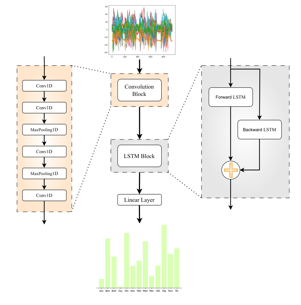
Figure 1 provides a schematic overview of the framework. The CRNN framework passes the output of the Convolutional Module to a Bi-Directional LSTM consisting of a single LSTM with 256 output units. The LSTM’s activation function is , and its recurrent activation is . The Attention Mechanism used in our framework is based on Hierarchical Attention Networks (Yang et al, 2016). In the Attention Mechanism, contexts of features are summarized with a bidirectional LSTM by going forward and backwards.
| (1a) | |||
| (1b) | |||
| (1c) |
In equation 1c, is the number of audio specimens. is the input sequence for the LSTM network. and provide the learned vectors from LSTM forward direction and backward direction, respectively. The vector, , builds the base for the attention mechanism. The goal of the attention mechanism is to learn the model through training with randomly initialized weights and biases. The layer also ensures with the function that the network does not stall. The function keeps the input values between -1 and 1 and maps zeros to near-zero values. The layer with function is again multiplied by trainable context vector . The trainable context vector refers to a vector learned during the training process and used as a fixed-length representation of the entire input document. In our framework, the attention mechanism is used to compute a weighted sum of the sequences for each speech utterance, where the weights are learned based on the relevance of each sequence to the speech utterances. This produces a fixed-length vector for each utterance that captures the most salient information in the sequences. The context weight vector is randomly initiated and jointly learned during the training process. Improved vectors are represented by as shown in equation 2.
| (2) |
Context vectors are finally calculated by providing a weight to each by dividing the exponential values of the previously generated vectors with the summation of all exponential values of previously generated vectors as shown in equation 3. To avoid division by zero, an epsilon is added to the denominator.
| (3) |
The sum of these importance weights concatenated with the previously calculated context vectors is fed to a linear layer with 13 output units serving as a classifier for the 13 languages.
Figure 2 presents the schematic diagram of the Attention Module where is the input to the module and output of the Bi-Directional LSTM layers.
4 Experiments
4.1 Feature Extraction
For feature extraction of spoken utterances, we used MFCCs. For calculating MFCCs we used , frame size represented as , frame stride represented as , N-point Fast Fourier transform represented as , low-frequency mel represented as , the number of filters represented as , the number of cepstral coefficients represented as and cepstral lifter represented of values 0.97, 0.025 (25ms), 0.015 (15ms overlapping), 512, 0, 40, 13, and 22, respectively. We used a frame size of 25 ms as typically frame sizes in the speech processing domain use 20ms to 40ms with 50% (in our case 15ms) overlapping between consecutive frames.
| (4) |
We used low-frequency mel (lf) as 0 and high-frequency mel (hf) is calculated using the equation 4. lf and hf are used to generate the non-linear human ear perception of sound, by being more discriminative at lower frequencies and less discriminative at higher frequencies.
| (5) |
As shown in equation 5 emphasized signal is calculated by using a pre-emphasis filter applied on the signal () using the first-order filter. The number of frames is calculated by taking the ceiling value of the division of the absolute value of the difference between signal length () and product of filter size () and sample rate (sr) with the product of frame stride () and sample rate (sr) as shown in equation 6. Signal length is the length of calculated in equation 5.
| (6) |
Using equation 7 is generated from concatenation of and zero value array of dimension ()1, where, is calculated by .
| (7) |
Frames are calculated as shown in equation 8 from the elements where elements are the addition of an array of positive natural numbers from 0 to repeated and the transpose of the array of size of where each element is the difference of .
| (8) |
Power frames shown in equation 9 are calculated as the square of the absolute value of the Discrete Fourier Transform (DFT) of the product of hamming window and frames of each element with NFFT.
| (9) |
| (10) |
Mel points are the array where elements are calculated as shown in the equation 10, where i is the values belonging from lf to hf.
| (11) |
From equation 11, bins are calculated where the floor value of the elements are taken which is the product of hertz points and divided by the sample rate. Hertz points are calculated by multiplying 700 by subtraction of 1 from 10 power of .
| (12) |
Bins calculated from equation 11 are used to calculate filter banks shown in equation 12. Each filter in the filter bank is triangular, with a response of 1 at the central frequency and a linear drop to 0 till it meets the central frequencies of the two adjacent filters, where the response is 0.
Finally, mfcc is calculated shown in equation 13 by decorrelating the filter bank coefficients using Discrete Cosine Transform (DCT) to get a compressed representation of the filter banks. Sinusoidal liftering is applied to the mfcc to de-emphasize higher mfccs which improves classification in noisy signals.
| (13) |
MFCCs features of shape generated from equation 13 is provided as input to the neural network which expects the same dimension followed by convolution layers as mentioned in section 3. Raw speech signal cannot be provided input to the framework as it contains lots of noise data therefore extracting features from the speech signal and using it as input to the model will produce better performance than directly considering raw speech signal as input. Our motivation to use MFCC features as the feature count is small enough to force us to learn the information of the sample. Parameters are related to the amplitude of frequencies and provide us with frequency channels to analyze the speech specimen.
4.2 Data
4.2.1 Benchmark Data
The Indian language (IL) dataset was acquired from the Indian Institute of Technology, Madras77 7 https://www.iitm.ac.in/donlab/tts/database.php. The dataset includes 13 widely used Indian languages. Table 2 presents the statistics of this dataset which we used for our experiments.
| Language | Label | Gender | Samples | Total Samples |
| ||
| Assamese | as | F | 8,713 | 17,654 | 5.587 | ||
| M | 8,941 | ||||||
| Bengali | bn | F | 3,253 | 9,440 | 5.743 | ||
| M | 6,187 | ||||||
| Bodo | bd | F | 571 | 571 | 25.219 | ||
| Gujarati | gu | F | 2,396 | 5,684 | 13.459 | ||
| M | 3,288 | ||||||
| Hindi | hi | F | 2,318 | 4,636 | 8.029 | ||
| M | 2,318 | ||||||
| Kannada | kn | F | 1,289 | 2,578 | 10.264 | ||
| M | 1,289 | ||||||
| Malayalam | ml | F | 5,650 | 11,300 | 5.699 | ||
| M | 5,650 | ||||||
| Manipuri | mn | F | 9,487 | 17,917 | 4.169 | ||
| M | 8,430 | ||||||
| Marathi | mr | F | 2,448 | 2,448 | 7.059 | ||
| Odia | or | F | 3,578 | 7,151 | 4.4 | ||
| M | 3,573 | ||||||
| Rajasthani | rj | F | 4,346 | 9,125 | 7.914 | ||
| M | 4,779 | ||||||
| Tamil | ta | F | 3,243 | 6,960 | 10.516 | ||
| M | 3,717 | ||||||
| Telugu | te | F | 4,043 | 6,524 | 15.395 | ||
| M | 2,481 |
4.2.2 Experimental Data
In the past two decades, the development of LID methods has been largely fostered through NIST Language Evaluations (LREs). As a result, the most popular benchmark for evaluating new LID models and methods is the NIST LRE evaluation dataset (Sadjadi et al, 2018). The NIST LREs dataset mostly contains narrow-band telephone speech. Datasets are typically distributed by the Linguistic Data Consortium (LDC) and cost thousands of dollars. For example, the standard Kaldi (Povey et al, 2011) recipe for LRE072 relies on 18 LDC SLR datasets that cost $15000 (approx) to LDC non-members. This makes it difficult for new research groups to enter the academic field of LID. Furthermore, the NIST LRE evaluations focus mostly on telephone speech.
| Language | Label | Total Samples |
| ||
|---|---|---|---|---|---|
| English | en | 43,269 | 684.264 | ||
| French | fr | 67,689 | 492.219 | ||
| German | de | 48,454 | 1,152.916 | ||
| Spanish | es | 57,869 | 798.169 |
As the NIST LRE dataset is not freely available we used the EU Dataset (Bartz et al, 2017) which is open source. The (EU) dataset contains YouTube News data for 4 major European languages – English (en), French (fr), German (de) and Spanish (es). Statistics of the dataset are given in Table 3.
4.3 Environment
We implemented our framework using Tensorflow (Abadi et al, 2016) backend. We split the Indian language dataset into training, validation, and testing set, containing 80%, 10%, and 10% of the data, respectively, for each language and gender.
For regularization, we apply dropout (Srivastava et al, 2014) after the Max-Pooling layer and Bi-Directional LSTM layer. We use the rate of 0.1. A regularization with weight is also added to all the trainable weights in the network. We train the model with Adam (Kingma et al, 2014) optimizer with , , and and learning rate schedule (Vaswani et al, 2017), with 4k warm-up steps and peak learning rate of where d is 128. A batch size of 64 with “Sparse Categorical Crossentropy” as the loss function was used.
4.4 Result on Indian Language Dataset
The proposed framework was assessed against Kulkarni et al, 2022 using identical datasets. Both CRNN and CRNN with Attention exhibited superior performance compared to the results reported by Kulkarni et al, 2022, as shown in Table 4. They used 6 Linear layers where units are 256, 256, 128, 64, 32, and 13, respectively in the CNN framework, whereas the DNN framework uses 3 LSTM layers having units 256, 256, and 128, respectively followed by dropout layer followed by 3 Time Distributed layer followed by a Linear layer of 13 as units.
| Accuracy | |
|---|---|
| DNN (Kulkarni et al, 2022) | 0.9834 |
| RNN (Kulkarni et al, 2022) | 0.9843 |
| CNN | 0.983 |
| CRNN | 0.987 |
| CRNN with Attention | 0.987 |
We evaluated system performance using the following evaluation metrics – Recall (TPR), Precision (PPV), f1-score, and Accuracy. Since one of our major objectives was to measure the accessibility of the network to new languages, we introduced Data Balancing of training data for each class, as the number of samples available for each class may vary drastically. This is the case for the Indian Language Dataset as shown in Table 2 in which Kannada, Marathi and particularly Bodo have a limited amount of data compared to the rest of the languages. To alleviate this data imbalance problem, we used class weight balancing as a dynamic method using scikit-learn (Pedregosa et al, 2011).
| Language | CRNN with Attention | CRNN | CNN | ||||||||||||||
| PPV | TPR |
|
Accuracy | PPV | TPR |
|
Accuracy | PPV | TPR |
|
Accuracy | ||||||
| as | 0.989 | 0.998 | 0.993 | 0.987 | 0.995 | 0.989 | 0.992 | 0.987 | 0.991 | 0.988 | 0.989 | 0.983 | |||||
| bn | 1 | 0.9 | 0.948 | 1 | 0.904 | 0.949 | 1 | 0.888 | 0.941 | ||||||||
| bd | 0.966 | 1 | 0.983 | 0.966 | 1 | 0.983 | 0.966 | 1 | 0.983 | ||||||||
| gu | 0.997 | 0.997 | 0.997 | 0.951 | 0.998 | 0.974 | 0.996 | 0.991 | 0.994 | ||||||||
| hi | 0.987 | 0.991 | 0.989 | 0.991 | 0.991 | 0.991 | 0.991 | 0.974 | 0.983 | ||||||||
| kn | 0.977 | 0.996 | 0.987 | 0.996 | 0.996 | 0.996 | 0.973 | 0.992 | 0.983 | ||||||||
| ml | 0.996 | 0.988 | 0.992 | 0.997 | 0.99 | 0.994 | 0.99 | 0.993 | 0.991 | ||||||||
| mn | 0.987 | 0.999 | 0.993 | 0.973 | 0.999 | 0.986 | 0.972 | 0.998 | 0.985 | ||||||||
| mr | 1 | 1 | 1 | 1 | 1 | 1 | 1 | 0.996 | 0.998 | ||||||||
| or | 1 | 1 | 1 | 1 | 0.999 | 0.999 | 0.986 | 0.999 | 0.992 | ||||||||
| rj | 0.999 | 0.993 | 0.996 | 0.995 | 1 | 0.997 | 0.986 | 0.996 | 0.991 | ||||||||
| ta | 0.929 | 0.991 | 0.959 | 0.975 | 0.997 | 0.986 | 0.946 | 0.989 | 0.967 | ||||||||
| te | 0.979 | 0.998 | 0.989 | 0.982 | 1 | 0.991 | 0.975 | 0.998 | 0.986 | ||||||||
PPV, TPR, f1-score, and Accuracy scores are reported in Table 5 for the three frameworks - CNN, CRNN, and CRNN with Attention. From Table 5 it is clearly visible that both CRNN framework and CRNN with Attention provide competitive results of 0.987 accuracy. Table 6, Table 7, and Table 8 shows the confusion matrix for CNN, CRNN, and CRNN with Attention.
| Predicted | PPV | TPR | f1 Score | ||||||||||||||
| as | bn | bd | gu | hi | kn | ml | mn | mr | or | rj | ta | te | |||||
| Actual | as | 1762 | 0 | 0 | 0 | 0 | 0 | 0 | 4 | 0 | 0 | 0 | 0 | 0 | 0.989 | 0.998 | 0.993 |
| bn | 10 | 850 | 0 | 1 | 0 | 0 | 0 | 18 | 0 | 0 | 0 | 53 | 12 | 1 | 0.9 | 0.948 | |
| bd | 0 | 0 | 57 | 0 | 0 | 0 | 0 | 0 | 0 | 0 | 0 | 0 | 0 | 0.966 | 1 | 0.983 | |
| gu | 1 | 0 | 0 | 566 | 0 | 0 | 0 | 0 | 0 | 0 | 0 | 0 | 1 | 0.997 | 0.997 | 0.997 | |
| hi | 0 | 0 | 0 | 0 | 460 | 0 | 4 | 0 | 0 | 0 | 0 | 0 | 0 | 0.987 | 0.991 | 0.989 | |
| kn | 0 | 0 | 1 | 0 | 0 | 257 | 0 | 0 | 0 | 0 | 0 | 0 | 0 | 0.977 | 0.996 | 0.987 | |
| ml | 0 | 0 | 1 | 0 | 6 | 5 | 1116 | 1 | 0 | 0 | 0 | 0 | 1 | 0.996 | 0.988 | 0.992 | |
| mn | 0 | 0 | 0 | 1 | 0 | 0 | 0 | 1790 | 0 | 0 | 0 | 0 | 0 | 0.987 | 0.999 | 0.993 | |
| mr | 0 | 0 | 0 | 0 | 0 | 0 | 0 | 0 | 245 | 0 | 0 | 0 | 0 | 1 | 1 | 1 | |
| or | 0 | 0 | 0 | 0 | 0 | 0 | 0 | 0 | 0 | 716 | 0 | 0 | 0 | 1 | 1 | 1 | |
| rj | 4 | 0 | 0 | 0 | 0 | 1 | 1 | 0 | 0 | 0 | 906 | 0 | 0 | 0.999 | 0.993 | 0.996 | |
| ta | 5 | 0 | 0 | 0 | 0 | 0 | 0 | 0 | 0 | 0 | 1 | 690 | 0 | 0.929 | 0.991 | 0.959 | |
| te | 0 | 0 | 0 | 0 | 0 | 0 | 0 | 1 | 0 | 0 | 0 | 0 | 652 | 0.979 | 0.998 | 0.989 | |
| Predicted | PPV | TPR | f1 Score | ||||||||||||||
| as | bn | bd | gu | hi | kn | ml | mn | mr | or | rj | ta | te | |||||
| Actual | as | 1746 | 0 | 0 | 0 | 0 | 0 | 0 | 19 | 0 | 0 | 0 | 1 | 0 | 0.995 | 0.989 | 0.992 |
| bn | 8 | 853 | 0 | 28 | 0 | 0 | 0 | 28 | 0 | 0 | 0 | 17 | 10 | 1 | 0.904 | 0.949 | |
| bd | 0 | 0 | 57 | 0 | 0 | 0 | 0 | 0 | 0 | 0 | 0 | 0 | 0 | 0.966 | 1 | 0.983 | |
| gu | 0 | 0 | 0 | 567 | 0 | 0 | 0 | 0 | 0 | 0 | 0 | 0 | 1 | 0.951 | 0.998 | 0.974 | |
| hi | 0 | 0 | 0 | 0 | 460 | 0 | 3 | 0 | 0 | 0 | 1 | 0 | 0 | 0.991 | 0.991 | 0.991 | |
| kn | 0 | 0 | 1 | 0 | 0 | 257 | 0 | 0 | 0 | 0 | 0 | 0 | 0 | 0.996 | 0.996 | 0.996 | |
| ml | 0 | 0 | 1 | 0 | 4 | 1 | 1119 | 1 | 0 | 0 | 4 | 0 | 0 | 0.997 | 0.99 | 0.994 | |
| mn | 0 | 0 | 0 | 1 | 0 | 0 | 0 | 1789 | 0 | 0 | 0 | 0 | 1 | 0.973 | 0.999 | 0.986 | |
| mr | 0 | 0 | 0 | 0 | 0 | 0 | 0 | 0 | 245 | 0 | 0 | 0 | 0 | 1 | 1 | 1 | |
| or | 0 | 0 | 0 | 0 | 0 | 0 | 0 | 1 | 0 | 715 | 0 | 0 | 0 | 1 | 0.999 | 0.999 | |
| rj | 0 | 0 | 0 | 0 | 0 | 0 | 0 | 0 | 0 | 0 | 912 | 0 | 0 | 0.995 | 1 | 0.997 | |
| ta | 1 | 0 | 0 | 0 | 0 | 0 | 0 | 1 | 0 | 0 | 0 | 694 | 0 | 0.975 | 0.997 | 0.986 | |
| te | 0 | 0 | 0 | 0 | 0 | 0 | 0 | 0 | 0 | 0 | 0 | 0 | 653 | 0.982 | 1 | 0.991 | |
| Predicted | PPV | TPR | f1 Score | ||||||||||||||
| as | bn | bd | gu | hi | kn | ml | mn | mr | or | rj | ta | te | |||||
| Actual | as | 1744 | 0 | 1 | 0 | 0 | 3 | 1 | 13 | 0 | 0 | 0 | 4 | 0 | 0.991 | 0.988 | 0.989 |
| bn | 9 | 838 | 0 | 1 | 1 | 0 | 0 | 35 | 0 | 8 | 5 | 34 | 13 | 1 | 0.888 | 0.941 | |
| bd | 0 | 0 | 57 | 0 | 0 | 0 | 0 | 0 | 0 | 0 | 0 | 0 | 0 | 0.966 | 1 | 0.983 | |
| gu | 2 | 0 | 0 | 563 | 0 | 0 | 0 | 0 | 0 | 1 | 0 | 0 | 2 | 0.996 | 0.991 | 0.994 | |
| hi | 0 | 0 | 0 | 0 | 452 | 0 | 10 | 0 | 0 | 0 | 2 | 0 | 0 | 0.991 | 0.974 | 0.983 | |
| kn | 0 | 0 | 0 | 0 | 1 | 256 | 0 | 0 | 0 | 0 | 1 | 0 | 0 | 0.973 | 0.992 | 0.983 | |
| ml | 0 | 0 | 1 | 0 | 2 | 2 | 1122 | 0 | 0 | 0 | 3 | 0 | 0 | 0.99 | 0.993 | 0.991 | |
| mn | 1 | 0 | 0 | 0 | 0 | 0 | 0 | 1788 | 0 | 0 | 0 | 1 | 1 | 0.972 | 0.998 | 0.985 | |
| mr | 0 | 0 | 0 | 0 | 0 | 0 | 0 | 0 | 244 | 1 | 0 | 0 | 0 | 1 | 0.996 | 0.998 | |
| or | 0 | 0 | 0 | 0 | 0 | 0 | 0 | 1 | 0 | 715 | 0 | 0 | 0 | 0.986 | 0.999 | 0.992 | |
| rj | 1 | 0 | 0 | 0 | 0 | 2 | 1 | 0 | 0 | 0 | 908 | 0 | 0 | 0.986 | 0.996 | 0.991 | |
| ta | 3 | 0 | 0 | 1 | 0 | 0 | 0 | 1 | 0 | 0 | 2 | 688 | 1 | 0.946 | 0.989 | 0.967 | |
| te | 0 | 0 | 0 | 0 | 0 | 0 | 0 | 1 | 0 | 0 | 0 | 0 | 652 | 0.975 | 0.998 | 0.986 | |
From Table 6, Table 7, and Table 8 it can be observed that Assamese gets confused with Manipuri; Bengali gets confused with Assamese, Manipuri, Tamil, and Telugu; and Hindi gets confused with Malayalam.
Assamese and Bengali have originated from the same language family and they share approximately the same phoneme set. However, Bengali and Tamil are from different language families but share a similar phoneme set. For example, in Bengali cigar is churut and star is nakshatra while cigar in Tamil is charuttu and star in Tamil is natsattira, which is quite similar. Similarly, Manipuri and Assamese share similar phonemes. On close study, we observed that Hindi and Malayalam have also similar phoneme sets as both languages borrowed most of the vocabulary from Sanskrit. For example, ‘arrogant’ is Ahankar in Hindi and Ahankaram in Malayalam. Similarly, Sathyu or commonly spoken as Satya in Hindi means ‘Truth’, which is Sathyam in Malayalam. Also, the word Sundar in Hindi is Sundaram in Malayalam, which means ‘beautiful’.
Table 9 shows the most common classification errors encountered during evaluation.
| Assamese | Manipuri | |
| Bengali | Assamese | |
| Bengali | Manipuri | |
| Bengali | Tamil | |
| Hindi | Malayalam |
4.5 Result on same language families on Indian Language Dataset
A deeper study into these 13 Indian languages led us to define five clusters of languages based on their phonetic similarity. Cluster internal languages are phonetically similar, close, and geographically contiguous, hence difficult to differentiate.
- •
Cluster 1: Assamese, Bengali, Odia
- •
Cluster 2: Gujarati, Hindi, Marathi, Rajasthani
- •
Cluster 3: Kannada, Malayalam, Tamil, Telugu
- •
Cluster 4: Bodo
- •
Cluster 5: Manipuri
Bodo and Manipuri are phonetically very much distant from any of the rest of the languages, thus they form singleton clusters. We carried out separate experiments for the identification of the cluster internal languages for Cluster 1, 2 and 3, and the experimental results are presented in Table 10.
| Cluster | Language |
|
CRNN | CNN | |||||||||||||
| PPV | TPR |
|
Accuracy | PPV | TPR |
|
Accuracy | PPV | TPR |
|
Accuracy | ||||||
| 1 | as | 0.962 | 1 | 0.981 | 0.98 | 0.953 | 1 | 0.976 | 0.974 | 0.953 | 1 | 0.976 | 0.971 | ||||
| bn | 1 | 0.926 | 0.961 | 1 | 0.907 | 0.951 | 1 | 0.894 | 0.944 | ||||||||
| or | 1 | 1 | 1 | 1 | 1 | 1 | 0.982 | 1 | 0.991 | ||||||||
| 2 | gu | 1 | 0.998 | 0.999 | 0.999 | 1 | 0.998 | 0.999 | 0.999 | 1 | 0.993 | 0.996 | 0.996 | ||||
| hi | 1 | 1 | 1 | 1 | 0.998 | 0.999 | 0.991 | 0.996 | 0.994 | ||||||||
| mr | 1 | 1 | 1 | 1 | 1 | 1 | 1 | 0.996 | 0.998 | ||||||||
| rj | 0.999 | 1 | 0.999 | 0.998 | 1 | 0.999 | 0.995 | 0.998 | 0.996 | ||||||||
| 3 | kn | 1 | 0.996 | 0.998 | 0.999 | 1 | 1 | 1 | 1 | 0.992 | 0.988 | 0.99 | 0.996 | ||||
| ml | 0.999 | 1 | 0.999 | 1 | 1 | 1 | 0.996 | 0.996 | 0.996 | ||||||||
| ta | 1 | 1 | 1 | 1 | 1 | 1 | 0.996 | 0.997 | 0.996 | ||||||||
| te | 1 | 1 | 1 | 1 | 1 | 1 | 0.995 | 0.997 | 0.996 | ||||||||
It can be clearly observed from Table 10 that both CRNN framework and CRNN with Attention provide competitive results for every language cluster. For cluster-1 CRNN framework and CRNN with Attention provides an accuracy of 0.98/0.974, for cluster-2 0.999/0.999, and for cluster-3 0.999/1, respectively. CNN framework also provides comparable results to the other two frameworks.
| CRNN and Attention | |||||||
| Predicted | PPV | TPR | f1 Score | ||||
| as | bn | or | |||||
| Actual | as | 1766 | 0 | 0 | 0.962 | 1 | 0.981 |
| bn | 70 | 874 | 0 | 1 | 0.926 | 0.961 | |
| or | 0 | 0 | 716 | 1 | 1 | 1 | |
| CRNN | |||||||
| Predicted | PPV | TPR | f1 Score | ||||
| as | bn | or | |||||
| Actual | as | 1766 | 0 | 0 | 0.953 | 1 | 0.976 |
| bn | 88 | 856 | 0 | 1 | 0.907 | 0.951 | |
| or | 0 | 0 | 716 | 1 | 1 | 1 | |
| CNN | |||||||
| Predicted | PPV | TPR | f1 Score | ||||
| as | bn | or | |||||
| Actual | as | 1766 | 0 | 0 | 0.953 | 1 | 0.976 |
| bn | 87 | 844 | 13 | 1 | 0.894 | 0.944 | |
| or | 0 | 0 | 716 | 0.982 | 1 | 0.991 | |
| CRNN and Attention | ||||||||
| Predicted | PPV | TPR | f1 Score | |||||
| gu | hi | mr | rj | |||||
| Actual | gu | 567 | 0 | 0 | 1 | 1 | 0.998 | 0.999 |
| hi | 0 | 464 | 0 | 0 | 1 | 1 | 1 | |
| mr | 0 | 0 | 245 | 0 | 1 | 1 | 1 | |
| rj | 0 | 0 | 0 | 912 | 0.999 | 1 | 0.999 | |
| CRNN | ||||||||
| Predicted | PPV | TPR | f1 Score | |||||
| gu | hi | mr | rj | |||||
| Actual | gu | 567 | 0 | 0 | 1 | 1 | 0.998 | 0.999 |
| hi | 0 | 463 | 0 | 1 | 1 | 0.998 | 0.999 | |
| mr | 0 | 0 | 245 | 0 | 1 | 1 | 1 | |
| rj | 0 | 0 | 0 | 912 | 0.998 | 1 | 0.999 | |
| CNN | ||||||||
| Predicted | PPV | TPR | f1 Score | |||||
| gu | hi | mr | rj | |||||
| Actual | gu | 564 | 2 | 0 | 2 | 1 | 0.993 | 0.996 |
| hi | 0 | 462 | 0 | 2 | 0.991 | 0.996 | 0.994 | |
| mr | 0 | 0 | 244 | 1 | 1 | 0.996 | 0.998 | |
| rj | 0 | 2 | 0 | 910 | 0.995 | 0.998 | 0.996 | |
| CRNN and Attention | ||||||||
| Predicted | PPV | TPR | f1 Score | |||||
| kn | ml | ta | te | |||||
| Actual | kn | 257 | 1 | 0 | 0 | 1 | 0.996 | 0.998 |
| ml | 0 | 1130 | 0 | 0 | 0.999 | 1 | 0.999 | |
| ta | 0 | 0 | 696 | 0 | 1 | 1 | 1 | |
| te | 0 | 0 | 0 | 653 | 1 | 1 | 1 | |
| CRNN | ||||||||
| Predicted | PPV | TPR | f1 Score | |||||
| kn | ml | ta | te | |||||
| Actual | kn | 258 | 0 | 0 | 0 | 1 | 1 | 1 |
| ml | 0 | 1130 | 0 | 0 | 1 | 1 | 1 | |
| ta | 0 | 0 | 696 | 0 | 1 | 1 | 1 | |
| te | 0 | 0 | 0 | 653 | 1 | 1 | 1 | |
| CNN | ||||||||
| Predicted | PPV | TPR | f1 Score | |||||
| kn | ml | ta | te | |||||
| Actual | kn | 255 | 3 | 0 | 0 | 0.992 | 0.988 | 0.99 |
| ml | 1 | 1125 | 2 | 2 | 0.996 | 0.996 | 0.996 | |
| ta | 1 | 0 | 694 | 1 | 0.996 | 0.997 | 0.996 | |
| te | 0 | 1 | 1 | 651 | 0.995 | 0.997 | 0.996 | |
Table 11, Table 13 and Table 13 presents the confusion matrix for cluster 1, cluster 2, and cluster 3, respectively. From Table 11, we observed that Bengali gets confused with Assamese and Odia, which is quite expected since these two languages are spoken in neighbouring states and both of them share almost the same phonemes. For example, in Odia rice is pronounced as bhata whereas in Bengali pronounced as bhat, similarly fish in odia as machha whereas in Bengali it is machh. Both CRNN and CRNN with Attention perform well to discriminate between Bengali and Odia. It can be observed from Table 13 that CNN creates a lot of confusion when discriminating between these four languages. Both CRNN and CRNN with Attention prove to be better at discriminating among these languages. From the results in Table 10, 11, 13 and 13, it is pretty clear that CRNN (Bi-Directional LSTM over CNN) and CRNN with Attention are more effective for Indian language identification and they perform almost at par. Another important observation is that it is harder to classify the languages in cluster 1 than in the other two clusters.
4.6 Results on European Language
We evaluated our model in two environments – No Noise and White Noise. According to our intuition, in real-life scenarios during prediction of language chances of capturing background noise of chatter and other sounds may happen. For the white noise evaluation setup, we mixed white noise into each test sample which has an audible solid presence but retains the identity of the language.
| No Noise | White Noise | |
|---|---|---|
| CRNN (Bartz et al, 2017) | 0.91 | 0.63 |
| Inception-v3 CRNN (Bartz et al, 2017) | 0.96 | 0.91 |
| CNN | 0.948 | 0.871 |
| CRNN | 0.967 | 0.912 |
| CRNN with Attention | 0.966 | 0.888 |
Table 14 compares the results of our models on the EU dataset with state-of-the-art models presented by Bartz et al, 2017. The model proposed by Bartz et al, 2017 consists of CRNN and uses Google’s Inception-v3 framework (Szegedy et al, 2016). The feature extractor performs convolutional operations on the input image through multiple stages, resulting in the production of a feature map that possesses a height of one. The feature map is partitioned horizontally along the x-axis, and each partition is employed as a temporal unit for the subsequent Bidirectional LSTM network. The network employs a total of five convolutional layers, with each layer being succeeded by the ReLU activation function, Batch Normalization, and max pooling with a stride of 2. The convolutional layers in question are characterized by their respective kernel sizes and the number of filters, which are as follows: (, 16), (, 32), (, 64), (, 128), and (, 256). The Bidirectional LSTM model comprises a pair of individual LSTM models, each with 256 output units. The concatenation of the two outputs is transformed into a 512-dimensional vector, which is then input into a fully-connected layer. The layer has either 4 or 6 output units, which function as the classifier. They experimented in four different environments – No Noise, White Noise, Cracking Noise, and Background Noise. All our evaluation results are rounded to 3 digits after the decimal point.
The CNN model failed to achieve competitive results; it provided an accuracy of 0.948/0.871 in No Noise/White Noise. In the CRNN framework, our model provides an accuracy of 0.967/0.912 on the No Noise/White Noise scenario outperforming the state-of-the-art results of Bartz et al, 2017. Use of Attention improves over the Inception-v3 CRNN in the No Noise scenario, however, it does not perform well on White Noise.
4.7 Ablation Studies
4.7.1 Convolution Kernel Size
To study the effect of kernel sizes in the convolution layers, we sweep the kernel size with 3, 7, 17, 32, and 65 of the models. We found that performance decreases with larger kernel sizes, as shown in Table 15. On comparing the accuracy up to the second decimal place kernel size 3 performs better than the rest.
| Kernel size | Accuracy |
|---|---|
| 3 | 98.7% |
| 7 | 98.68% |
| 17 | 98.65% |
| 32 | 98.13% |
| 65 | 93.56% |
4.7.2 Automatic Class Weight vs Manual Class Weight
Balancing the data using class weights gives better accuracy for CRNN with Attention (98.7%) and CRNN (98.7%), compared to CNN (98.3%) shown in Table 5. We study the efficacy of the frameworks by manually balancing the datasets using 100 samples, 200 samples, and 571 samples drawn randomly from the dataset and the results of these experiments are presented in Table 16, Table 17 and Table 18, respectively.
| Language | CRNN with Attention | CRNN | CNN | ||||||||||||||
| PPV | TPR |
|
Accuracy | PPV | TPR |
|
Accuracy | PPV | TPR |
|
Accuracy | ||||||
| as | 0.766 | 0.72 | 0.742 | 0.883 | 0.839 | 0.94 | 0.887 | 0.932 | 0.617 | 0.58 | 0.598 | 0.72 | |||||
| bn | 0.875 | 0.7 | 0.778 | 0.957 | 0.9 | 0.928 | 0.816 | 0.8 | 0.808 | ||||||||
| bd | 1 | 1 | 1 | 0.962 | 1 | 0.98 | 0.843 | 0.86 | 0.851 | ||||||||
| gu | 0.943 | 1 | 0.971 | 1 | 0.98 | 0.99 | 0.731 | 0.76 | 0.745 | ||||||||
| hi | 0.959 | 0.94 | 0.95 | 0.957 | 0.9 | 0.928 | 0.778 | 0.7 | 0.737 | ||||||||
| kn | 0.961 | 0.98 | 0.97 | 0.94 | 0.94 | 0.94 | 0.725 | 0.74 | 0.733 | ||||||||
| ml | 0.958 | 0.92 | 0.939 | 0.923 | 0.96 | 0.941 | 0.774 | 0.82 | 0.796 | ||||||||
| mn | 0.878 | 0.72 | 0.791 | 0.935 | 0.86 | 0.896 | 0.691 | 0.76 | 0.724 | ||||||||
| mr | 0.906 | 0.96 | 0.932 | 0.98 | 0.96 | 0.97 | 0.857 | 0.84 | 0.848 | ||||||||
| or | 0.959 | 0.94 | 0.949 | 0.943 | 1 | 0.971 | 0.811 | 0.86 | 0.835 | ||||||||
| rj | 0.782 | 0.86 | 0.819 | 0.894 | 0.84 | 0.866 | 0.605 | 0.52 | 0.559 | ||||||||
| ta | 0.677 | 0.88 | 0.765 | 0.898 | 0.88 | 0.889 | 0.564 | 0.62 | 0.590 | ||||||||
| te | 0.878 | 0.86 | 0.869 | 0.906 | 0.96 | 0.932 | 0.532 | 0.5 | 0.515 | ||||||||
| Language | CRNN with Attention | CRNN | CNN | ||||||||||||||
| PPV | TPR |
|
Accuracy | PPV | TPR |
|
Accuracy | PPV | TPR |
|
Accuracy | ||||||
| as | 0.941 | 0.96 | 0.95 | 0.975 | 1 | 0.94 | 0.969 | 0.971 | 0.8 | 0.88 | 0.838 | 0.883 | |||||
| bn | 0.909 | 1 | 0.952 | 1 | 0.96 | 0.98 | 0.92 | 0.92 | 0.92 | ||||||||
| bd | 0.98 | 0.96 | 0.97 | 0.98 | 0.98 | 0.98 | 0.94 | 0.94 | 0.94 | ||||||||
| gu | 1 | 1 | 1 | 1 | 1 | 1 | 0.918 | 0.9 | 0.909 | ||||||||
| hi | 1 | 0.98 | 0.99 | 1 | 0.98 | 0.99 | 0.956 | 0.86 | 0.905 | ||||||||
| kn | 1 | 0.98 | 0.99 | 1 | 0.98 | 0.99 | 0.878 | 0.86 | 0.869 | ||||||||
| ml | 0.962 | 1 | 0.98 | 0.893 | 1 | 0.943 | 0.896 | 0.86 | 0.878 | ||||||||
| mn | 0.979 | 0.92 | 0.948 | 0.907 | 0.98 | 0.942 | 0.754 | 0.92 | 0.829 | ||||||||
| mr | 0.98 | 0.98 | 0.98 | 0.98 | 0.96 | 0.97 | 0.956 | 0.86 | 0.905 | ||||||||
| or | 0.98 | 1 | 0.99 | 1 | 1 | 1 | 0.941 | 0.96 | 0.95 | ||||||||
| rj | 0.96 | 0.96 | 0.96 | 1 | 0.96 | 0.98 | 0.86 | 0.86 | 0.86 | ||||||||
| ta | 1 | 0.96 | 0.98 | 0.904 | 0.94 | 0.922 | 0.784 | 0.8 | 0.792 | ||||||||
| te | 1 | 0.98 | 0.99 | 0.979 | 0.94 | 0.959 | 0.935 | 0.86 | 0.896 | ||||||||
| Language | CRNN with Attention | CRNN | CNN | ||||||||||||||
| PPV | TPR |
|
Accuracy | PPV | TPR |
|
Accuracy | PPV | TPR |
|
Accuracy | ||||||
| as | 1 | 1 | 1 | 0.988 | 0.983 | 0.983 | 0.983 | 0.985 | 0.967 | 1 | 0.983 | 0.945 | |||||
| bn | 1 | 1 | 1 | 1 | 1 | 1 | 0.983 | 1 | 0.991 | ||||||||
| bd | 1 | 1 | 1 | 1 | 1 | 1 | 1 | 1 | 1 | ||||||||
| gu | 1 | 1 | 1 | 0.983 | 1 | 0.991 | 0.982 | 0.931 | 0.956 | ||||||||
| hi | 0.983 | 0.983 | 0.983 | 1 | 1 | 1 | 0.893 | 0.862 | 0.877 | ||||||||
| kn | 1 | 1 | 1 | 1 | 1 | 1 | 0.903 | 0.966 | 0.933 | ||||||||
| ml | 1 | 0.966 | 0.982 | 0.983 | 1 | 0.991 | 0.914 | 0.914 | 0.914 | ||||||||
| mn | 0.983 | 1 | 0.991 | 1 | 0.983 | 0.991 | 0.931 | 0.931 | 0.931 | ||||||||
| mr | 1 | 1 | 1 | 0.982 | 1 | 0.991 | 0.965 | 0.982 | 0.973 | ||||||||
| or | 1 | 1 | 1 | 1 | 0.983 | 0.991 | 1 | 0.966 | 0.982 | ||||||||
| rj | 0.919 | 0.983 | 0.95 | 0.918 | 0.966 | 0.941 | 0.9 | 0.931 | 0.915 | ||||||||
| ta | 0.964 | 0.931 | 0.947 | 0.964 | 0.914 | 0.938 | 0.879 | 0.879 | 0.879 | ||||||||
| te | 1 | 0.983 | 0.991 | 1 | 0.983 | 0.991 | 0.982 | 0.931 | 0.956 | ||||||||
The objective of the study was to observe the performance of the frameworks in increasing the sample size. Since the Bodo language has the minimum data (571 samples) among all the languages in the dataset, we performed our experiments on 571 samples.
A comparison of the results in Table 16, Table 17, and Table 18 reveals the following observations.
- •
All the models perform consistently better with more training data.
- •
CRNN and CRNN with attention perform consistently better than CNN.
- •
CRNN is less data hungry among the 3 models and it performs the best in the lowest data scenario.

4.7.3 Additional performance and parameter size analysis of our frameworks
| Framework | CNN | CRNN |
| ||||
|---|---|---|---|---|---|---|---|
| Parameters | 1,355,917 | 2,094,477 | 2,357,645 | ||||
| Indian Dataset | 0.983 | 0.987 | 0.987 | ||||
| Close Language Cluster | Cluster 1 | 0.971 | 0.974 | 0.980 | |||
| Cluster 2 | 0.996 | 0.999 | 0.999 | ||||
| Cluster 3 | 0.996 | 1 | 0.999 | ||||
| European Language Dataset | No Noise | 0.948 | 0.967 | 0.966 | |||
| White Noise | 0.871 | 0.912 | 0.888 | ||||
Table 19 demonstrates that both CRNN and CRNN with attention perform better compared to the CNN-based framework. At the same time, CRNN itself produces better or equivalent performance compared to CRNN with an Attention-based mechanism. CRNN with Attention performs better only for Cluster 1 of the Indian dataset; CRNN itself produces the best results in all other tasks, sometimes jointly with CRNN with Attention. This is despite the fact that the Attention-based framework has more parameters than the other models. The underlying intuition is that the attention-based framework generally suffers from overfitting problems due to its additional parameter count. An attention-based framework needs to learn how to assign importance to different parts of the input sequence, which may require a large number of training instances to produce a generalized performance. Thus, CRNN with Attention makes the experimental set-up time-consuming and resource-intensive, but still, it is not able to improve over CRNN.
5 Conclusion and future work
In this work, we proposed a language identification method using CRNN that works on MFCC features of speech signals. Our framework efficiently identifies the language both in close language and noisy scenarios. We carried out extensive experiments and our framework produced state-of-the-art results. Through our experiments, we have also shown our framework’s robustness to noise and its extensibility to new languages. The model exhibits the overall best accuracy of 98.7% which improves over the traditional use of CNN (98.3%). CRNN with attention performs almost at par with CRNN, however, the attention mechanism which incurs additional computational overhead does not result in improvement over CRNN in most cases.
In future, we would like to extend our work by increasing the language classes with speech specimens recorded in different environments. We would also like to extend our work to check the usefulness of the proposed framework on smaller time speech samples through which we can deduce the optimal time required to classify the languages with high accuracy. We would also like to test our method on language dialect identification.
Acknowledgements
This research was supported by the TPU Research Cloud (TRC) program, a Google Research initiative and funded by Rashtriya Uchchatar Shiksha Abhiyan 2.0 [grant number R-11/828/19].
References
- Aarti et al, (2017) B. Aarti and S. K. Kopparapu, ”Spoken Indian language classification using artificial neural network — An experimental study,” 2017 4th International Conference on Signal Processing and Integrated Networks (SPIN), 2017, pp. 424-430, doi: 10.1109/SPIN.2017.8049987.
- Abadi et al, (2016) Martín Abadi, Paul Barham, Jianmin Chen, Zhifeng Chen, Andy Davis, Jeffrey Dean, Matthieu Devin, Sanjay Ghemawat, Geoffrey Irving, Michael Isard, Manjunath Kudlur, Josh Levenberg, Rajat Monga, Sherry Moore, Derek G. Murray, Benoit Steiner, Paul Tucker, Vijay Vasudevan, Pete Warden, Martin Wicke, Yuan Yu, and Xiaoqiang Zheng. 2016. TensorFlow: a system for large-scale machine learning. In Proceedings of the 12th USENIX conference on Operating Systems Design and Implementation (OSDI’16). USENIX Association, USA, 265–283.
- Bartz et al, (2017) Bartz, C., Herold, T., Yang, H., Meinel, C. (2017). Language Identification Using Deep Convolutional Recurrent Neural Networks. In: Liu, D., Xie, S., Li, Y., Zhao, D., El-Alfy, ES. (eds) Neural Information Processing. ICONIP 2017. Lecture Notes in Computer Science(), vol 10639. Springer, Cham. https://doi.org/10.1007/978-3-319-70136-3_93
- Chen et al, (2020) Chen, Pinzhen & Heafield, Kenneth. (2020). Approaching Neural Chinese Word Segmentation as a Low-Resource Machine Translation Task.
- Dehak et al, (2011) N. Dehak, P. J. Kenny, R. Dehak, P. Dumouchel and P. Ouellet, ”Front-End Factor Analysis for Speaker Verification,” in IEEE Transactions on Audio, Speech, and Language Processing, vol. 19, no. 4, pp. 788-798, May 2011, doi: 10.1109/TASL.2010.2064307.
- Dehak et al, (2011) Dehak, N., Torres-Carrasquillo, P.A., Reynolds, D., Dehak, R. (2011) Language recognition via i-vectors and dimensionality reduction. Proc. Interspeech 2011, 857-860, doi: 10.21437/Interspeech.2011-328
- Devlin et al, (2019) Jacob Devlin, Ming-Wei Chang, Kenton Lee, and Kristina Toutanova. 2019. BERT: Pre-training of Deep Bidirectional Transformers for Language Understanding. In Proceedings of the 2019 Conference of the North American Chapter of the Association for Computational Linguistics: Human Language Technologies, Volume 1 (Long and Short Papers), pages 4171–4186, Minneapolis, Minnesota. Association for Computational Linguistics.
- Draghichi et al, (2020) Alexandra Draghici, Jakob Abeßer, and Hanna Lukashevich. 2020. A study on spoken language identification using deep neural networks. In Proceedings of the 15th International Audio Mostly Conference (AM ’20). Association for Computing Machinery, New York, NY, USA, 253–256. https://doi.org/10.1145/3411109.3411123
- Ferrer et al, (2010) L. Ferrer, N. Scheffer and E. Shriberg, ”A comparison of approaches for modeling prosodic features in speaker recognition,” 2010 IEEE International Conference on Acoustics, Speech and Signal Processing, 2010, pp. 4414-4417, doi: 10.1109/ICASSP.2010.5495632.
- Ganapathy et al, (2014) Ganapathy, S., Han, K., Thomas, S., Omar, M., Segbroeck, M.V., Narayanan, S.S. (2014) Robust language identification using convolutional neural network features. Proc. Interspeech 2014, 1846-1850, doi: 10.21437/Interspeech.2014-419
- Gazeau et al, (2018) Valentin Gazeau, Cihan Varol, ”Automatic Spoken Language Recognition with Neural Networks”, International Journal of Information Technology and Computer Science(IJITCS), Vol.10, No.8, pp.11-17, 2018. DOI: 10.5815/ijitcs.2018.08.02
- Gelly et al, (2016) Gelly, G., Gauvain, J.-L., Le, V.B., Messaoudi, A. (2016) A Divide-and-Conquer Approach for Language Identification Based on Recurrent Neural Networks. Proc. Interspeech 2016, 3231-3235, doi: 10.21437/Interspeech.2016-180
- Gu et al, (2019) Jiatao Gu, Changhan Wang, and Jake Zhao Junbo. 2019. Levenshtein transformer. Proceedings of the 33rd International Conference on Neural Information Processing Systems. Curran Associates Inc., Red Hook, NY, USA, Article 1003, 11181–11191.
- He et al, (2016) K. He, X. Zhang, S. Ren and J. Sun, ”Deep Residual Learning for Image Recognition,” 2016 IEEE Conference on Computer Vision and Pattern Recognition (CVPR), 2016, pp. 770-778, doi: 10.1109/CVPR.2016.90.
- Heracleous et al, (2018) P. Heracleous, K. Takai, K. Yasuda, Y. Mohammad and A. Yoneyama, ”Comparative Study on Spoken Language Identification Based on Deep Learning,” 2018 26th European Signal Processing Conference (EUSIPCO), 2018, pp. 2265-2269, doi: 10.23919/EUSIPCO.2018.8553347.
- Howard et al, (2020) Howard, J.; Gugger, S. Fastai: A Layered API for Deep Learning. Information 2020, 11, 108. https://doi.org/10.3390/info11020108
- Joshi et al, (2020) Joshi, M., Chen, D., Liu, Y., Weld, D., Zettlemoyer, L., & Levy, O. (2020). SpanBERT: Improving Pre-training by Representing and Predicting Spans. Transactions of the Association for Computational Linguistics, 8, 64-77. Retrieved from https://transacl.org/ojs/index.php/tacl/article/view/1853
- Kingma et al, (2014) Kingma, Diederik P., and Jimmy Ba. ”Adam: A method for stochastic optimization.” arXiv preprint arXiv:1412.6980 (2014).
- Kulkarni et al, (2022) Kulkarni, R., Joshi, A., Kamble, M., Apte, S. (2022). Spoken Language Identification for Native Indian Languages Using Deep Learning Techniques. In: Chen, J.IZ., Wang, H., Du, KL., Suma, V. (eds) Machine Learning and Autonomous Systems. Smart Innovation, Systems and Technologies, vol 269. Springer, Singapore. https://doi.org/10.1007/978-981-16-7996-4_7
- Zhenzong et al, (2020) Zhenzhong, Lan., Mingda, Chen., Sebastian, Goodman., Kevin, Gimpel., Piyush, Sharma., Radu, Soricut. ALBERT: A Lite BERT for Self-supervised Learning of Language Representations. (2020).
- Lopez-Moreno et al, (2014) I. Lopez-Moreno, J. Gonzalez-Dominguez, O. Plchot, D. Martinez, J. Gonzalez-Rodriguez and P. Moreno, ”Automatic language identification using deep neural networks,” 2014 IEEE International Conference on Acoustics, Speech and Signal Processing (ICASSP), 2014, pp. 5337-5341, doi: 10.1109/ICASSP.2014.6854622.
- Lozano-Diez et al, (2015) Lozano-Diez, A., Zazo-Candil, R., Gonzalez-Dominguez, J., Toledano, D.T., Gonzalez-Rodriguez, J. (2015) An end-to-end approach to language identification in short utterances using convolutional neural networks. Proc. Interspeech 2015, 403-407, doi: 10.21437/Interspeech.2015-164
- Martinez et al, (2020) Martínez, D., Plchot, O., Burget, L., Glembek, O., Matějka, P. (2011) Language recognition in ivectors space. Proc. Interspeech 2011, 861-864, doi: 10.21437/Interspeech.2011-329
- Mukherjee et al, (2019) S. Mukherjee, N. Shivam, A. Gangwal, L. Khaitan and A. J. Das, ”Spoken Language Recognition Using CNN,” 2019 International Conference on Information Technology (ICIT), 2019, pp. 37-41, doi: 10.1109/ICIT48102.2019.00013.
- Nair and Geoffrey, (2010) Vinod Nair and Geoffrey E. Hinton. 2010. Rectified linear units improve restricted boltzmann machines. In Proceedings of the 27th International Conference on International Conference on Machine Learning (ICML’10). Omnipress, Madison, WI, USA, 807–814.
- Pedregosa et al, (2011) Fabian Pedregosa, Gaël Varoquaux, Alexandre Gramfort, Vincent Michel, Bertrand Thirion, Olivier Grisel, Mathieu Blondel, Peter Prettenhofer, Ron Weiss, Vincent Dubourg, Jake Vanderplas, Alexandre Passos, David Cournapeau, Matthieu Brucher, Matthieu Perrot, and Édouard Duchesnay. 2011. Scikit-learn: Machine Learning in Python. J. Mach. Learn. Res. 12, null (2/1/2011), 2825–2830.
- Plchot et al, (2016) Plchot, O., Matejka, P., Glembek, O., Fer, R., Novotny, O., Pesan, J., Burget, L., Brummer, N., Cumani, S. (2016) BAT System Description for NIST LRE 2015. Proc. The Speaker and Language Recognition Workshop (Odyssey 2016), 166-173, doi: 10.21437/Odyssey.2016-24
- Povey et al, (2011) Povey, Daniel & Ghoshal, Arnab & Boulianne, Gilles & Burget, Lukáš & Glembek, Ondrej & Goel, Nagendra & Hannemann, Mirko & Motlíček, Petr & Qian, Yanmin & Schwarz, Petr & Silovský, Jan & Stemmer, Georg & Vesel, Karel. (2011). The Kaldi speech recognition toolkit. IEEE 2011 Workshop on Automatic Speech Recognition and Understanding.
- Revay and Teschke, (2019) Revay, S., & Teschke, M. (2019). Multiclass Language Identification using Deep Learning on Spectral Images of Audio Signals. ArXiv, abs/1905.04348.
- Sadjadi et al, (2018) Sadjadi, S.O., Kheyrkhah, T., Greenberg, C., Singer, E., Reynolds, D., Mason, L., Hernandez-Cordero, J. (2018) Performance Analysis of the 2017 NIST Language Recognition Evaluation. Proc. Interspeech 2018, 1798-1802, doi: 10.21437/Interspeech.2018-69
- Sisodia et al, (2020) D. S. Sisodia, S. Nikhil, G. S. Kiran and P. Sathvik, ”Ensemble Learners for Identification of Spoken Languages using Mel Frequency Cepstral Coefficients,” 2nd International Conference on Data, Engineering and Applications (IDEA), 2020, pp. 1-5, doi: 10.1109/IDEA49133.2020.9170720.
- Smith, (2018) Smith, L.N. (2018). A disciplined approach to neural network hyper-parameters: Part 1 - learning rate, batch size, momentum, and weight decay. ArXiv, abs/1803.09820.
- Srivastava et al, (2014) Nitish Srivastava, Geoffrey Hinton, Alex Krizhevsky, Ilya Sutskever, and Ruslan Salakhutdinov. 2014. Dropout: a simple way to prevent neural networks from overfitting. J. Mach. Learn. Res. 15, 1 (January 2014), 1929–1958.
- Szegedy et al, (2016) C. Szegedy, V. Vanhoucke, S. Ioffe, J. Shlens and Z. Wojna, ”Rethinking the Inception Architecture for Computer Vision,” 2016 IEEE Conference on Computer Vision and Pattern Recognition (CVPR), 2016, pp. 2818-2826, doi: 10.1109/CVPR.2016.308.
- Takase et al, (2021) Takase, S., & Kiyono, S. (2021). Lessons on Parameter Sharing across Layers in Transformers. ArXiv, abs/2104.06022.
- Vaswani et al, (2017) Ashish Vaswani, Noam Shazeer, Niki Parmar, Jakob Uszkoreit, Llion Jones, Aidan N. Gomez, Łukasz Kaiser, and Illia Polosukhin. 2017. Attention is all you need. In Proceedings of the 31st International Conference on Neural Information Processing Systems (NIPS’17). Curran Associates Inc., Red Hook, NY, USA, 6000–6010.
- Venkatesan et al, (2018) H. Venkatesan, T. V. Venkatasubramanian and J. Sangeetha, ”Automatic Language Identification using Machine learning Techniques,” 2018 3rd International Conference on Communication and Electronics Systems (ICCES), 2018, pp. 583-588, doi: 10.1109/CESYS.2018.8724070.
- Yamada et al, (2020) Ikuya Yamada, Akari Asai, Hiroyuki Shindo, Hideaki Takeda, and Yuji Matsumoto. 2020. LUKE: Deep Contextualized Entity Representations with Entity-aware Self-attention. In Proceedings of the 2020 Conference on Empirical Methods in Natural Language Processing (EMNLP), pages 6442–6454, Online. Association for Computational Linguistics.
- Yang et al, (2019) Zhilin Yang, Zihang Dai, Yiming Yang, Jaime Carbonell, Ruslan Salakhutdinov, and Quoc V. Le. 2019. XLNet: generalized autoregressive pretraining for language understanding. Proceedings of the 33rd International Conference on Neural Information Processing Systems. Curran Associates Inc., Red Hook, NY, USA, Article 517, 5753–5763.
- Yang et al, (2016) Zichao Yang, Diyi Yang, Chris Dyer, Xiaodong He, Alex Smola, and Eduard Hovy. 2016. Hierarchical Attention Networks for Document Classification. In Proceedings of the 2016 Conference of the North American Chapter of the Association for Computational Linguistics: Human Language Technologies, pages 1480–1489, San Diego, California. Association for Computational Linguistics.
- Zazo et al, (2016) Zazo R, Lozano-Diez A, Gonzalez-Dominguez J, T. Toledano D, Gonzalez-Rodriguez J (2016) Language Identification in Short Utterances Using Long Short-Term Memory (LSTM) Recurrent Neural Networks. PLOS ONE 11(1): e0146917. https://doi.org/10.1371/journal.pone.0146917
- Zissman, (1996) M. A. Zissman, ”Comparison of four approaches to automatic language identification of telephone speech,” in IEEE Transactions on Speech and Audio Processing, vol. 4, no. 1, pp. 31-, Jan. 1996, doi: 10.1109/TSA.1996.481450.
Appendix A CNN framework
| Predicted | PPV | TPR | f1 Score | ||||||||||||||
| as | bn | bd | gu | hi | kn | ml | mn | mr | or | rj | ta | te | |||||
| Actual | as | 29 | 2 | 0 | 1 | 0 | 3 | 0 | 7 | 0 | 0 | 3 | 2 | 3 | 0.617 | 0.58 | 0.598 |
| bn | 2 | 40 | 0 | 0 | 0 | 1 | 1 | 1 | 1 | 0 | 0 | 3 | 1 | 0.816 | 0.8 | 0.808 | |
| bd | 0 | 0 | 43 | 1 | 0 | 2 | 0 | 0 | 2 | 0 | 1 | 1 | 0 | 0.843 | 0.86 | 0.851 | |
| gu | 1 | 0 | 0 | 38 | 4 | 0 | 0 | 0 | 0 | 0 | 0 | 3 | 4 | 0.731 | 0.76 | 0.745 | |
| hi | 2 | 0 | 0 | 2 | 35 | 3 | 3 | 0 | 0 | 2 | 0 | 2 | 1 | 0.778 | 0.7 | 0.737 | |
| kn | 0 | 0 | 1 | 0 | 1 | 37 | 6 | 1 | 0 | 0 | 1 | 0 | 3 | 0.725 | 0.74 | 0.733 | |
| ml | 0 | 1 | 0 | 1 | 0 | 3 | 41 | 0 | 0 | 0 | 2 | 1 | 1 | 0.774 | 0.82 | 0.796 | |
| mn | 2 | 2 | 0 | 0 | 0 | 0 | 1 | 38 | 0 | 1 | 0 | 1 | 5 | 0.691 | 0.76 | 0.724 | |
| mr | 0 | 0 | 1 | 0 | 0 | 0 | 0 | 0 | 42 | 3 | 4 | 0 | 0 | 0.857 | 0.84 | 0.848 | |
| or | 0 | 1 | 1 | 0 | 0 | 0 | 0 | 0 | 3 | 43 | 1 | 1 | 0 | 0.811 | 0.86 | 0.835 | |
| rj | 2 | 2 | 3 | 1 | 3 | 0 | 1 | 2 | 1 | 2 | 26 | 7 | 0 | 0.605 | 0.52 | 0.559 | |
| ta | 5 | 0 | 0 | 3 | 2 | 0 | 0 | 3 | 0 | 0 | 2 | 31 | 4 | 0.564 | 0.62 | 0.590 | |
| te | 4 | 1 | 2 | 5 | 0 | 2 | 0 | 3 | 0 | 2 | 3 | 3 | 25 | 0.532 | 0.5 | 0.515 | |
| Predicted | PPV | TPR | f1 Score | ||||||||||||||
| as | bn | bd | gu | hi | kn | ml | mn | mr | or | rj | ta | te | |||||
| Actual | as | 44 | 1 | 0 | 0 | 0 | 0 | 0 | 1 | 0 | 0 | 1 | 3 | 0 | 0.8 | 0.88 | 0.838 |
| bn | 1 | 46 | 0 | 0 | 0 | 0 | 0 | 1 | 0 | 0 | 0 | 2 | 0 | 0.92 | 0.92 | 0.92 | |
| bd | 0 | 0 | 47 | 0 | 0 | 1 | 0 | 1 | 0 | 0 | 1 | 0 | 0 | 0.94 | 0.94 | 0.94 | |
| gu | 1 | 1 | 0 | 45 | 1 | 0 | 0 | 0 | 0 | 0 | 0 | 0 | 2 | 0.918 | 0.9 | 0.909 | |
| hi | 0 | 1 | 0 | 1 | 43 | 1 | 1 | 2 | 0 | 0 | 1 | 0 | 0 | 0.956 | 0.86 | 0.905 | |
| kn | 0 | 0 | 1 | 1 | 0 | 43 | 2 | 1 | 0 | 0 | 0 | 1 | 1 | 0.878 | 0.86 | 0.869 | |
| ml | 1 | 0 | 0 | 0 | 0 | 1 | 43 | 2 | 1 | 2 | 0 | 0 | 0 | 0.896 | 0.86 | 0.878 | |
| mn | 2 | 0 | 0 | 0 | 0 | 0 | 1 | 46 | 0 | 0 | 0 | 1 | 0 | 0.754 | 0.92 | 0.829 | |
| mr | 0 | 0 | 2 | 0 | 0 | 0 | 1 | 1 | 43 | 1 | 2 | 0 | 0 | 0.956 | 0.86 | 0.905 | |
| or | 0 | 0 | 0 | 0 | 1 | 0 | 0 | 0 | 0 | 48 | 1 | 0 | 0 | 0.941 | 0.96 | 0.95 | |
| rj | 2 | 1 | 0 | 0 | 0 | 1 | 0 | 1 | 1 | 0 | 43 | 1 | 0 | 0.86 | 0.86 | 0.86 | |
| ta | 2 | 0 | 0 | 1 | 0 | 2 | 0 | 4 | 0 | 0 | 1 | 40 | 0 | 0.784 | 0.8 | 0.792 | |
| te | 2 | 0 | 0 | 1 | 0 | 0 | 0 | 1 | 0 | 0 | 0 | 3 | 43 | 0.935 | 0.86 | 0.896 | |
| Predicted | PPV | TPR | f1 Score | ||||||||||||||
| as | bn | bd | gu | hi | kn | ml | mn | mr | or | rj | ta | te | |||||
| Actual | as | 58 | 0 | 0 | 0 | 0 | 0 | 0 | 0 | 0 | 0 | 0 | 0 | 0 | 0.967 | 1 | 0.983 |
| bn | 0 | 58 | 0 | 0 | 0 | 0 | 0 | 0 | 0 | 0 | 0 | 0 | 0 | 0.983 | 1 | 0.991 | |
| bd | 0 | 0 | 56 | 0 | 0 | 0 | 0 | 0 | 0 | 0 | 0 | 0 | 0 | 1 | 1 | 1 | |
| gu | 0 | 0 | 0 | 54 | 4 | 0 | 0 | 0 | 0 | 0 | 0 | 0 | 0 | 0.982 | 0.931 | 0.956 | |
| hi | 0 | 0 | 0 | 0 | 50 | 0 | 2 | 1 | 0 | 0 | 0 | 5 | 0 | 0.893 | 0.862 | 0.877 | |
| kn | 0 | 0 | 0 | 0 | 0 | 56 | 2 | 0 | 0 | 0 | 0 | 0 | 0 | 0.903 | 0.966 | 0.933 | |
| ml | 0 | 0 | 0 | 0 | 0 | 4 | 53 | 0 | 0 | 0 | 1 | 0 | 0 | 0.914 | 0.914 | 0.914 | |
| mn | 1 | 0 | 0 | 0 | 0 | 1 | 0 | 54 | 0 | 0 | 0 | 1 | 1 | 0.931 | 0.931 | 0.931 | |
| mr | 0 | 0 | 0 | 0 | 0 | 0 | 0 | 0 | 55 | 0 | 1 | 0 | 0 | 0.965 | 0.982 | 0.973 | |
| or | 0 | 0 | 0 | 0 | 1 | 0 | 0 | 0 | 1 | 56 | 0 | 0 | 0 | 1 | 0.966 | 0.982 | |
| rj | 1 | 1 | 0 | 0 | 0 | 0 | 1 | 1 | 0 | 0 | 54 | 0 | 0 | 0.9 | 0.931 | 0.915 | |
| ta | 0 | 0 | 0 | 1 | 1 | 0 | 0 | 1 | 1 | 0 | 3 | 51 | 0 | 0.879 | 0.879 | 0.879 | |
| te | 0 | 0 | 0 | 0 | 0 | 1 | 0 | 1 | 0 | 0 | 1 | 1 | 54 | 0.982 | 0.931 | 0.956 | |
Appendix B CRNN framework
| Predicted | PPV | TPR | f1 Score | ||||||||||||||
| as | bn | bd | gu | hi | kn | ml | mn | mr | or | rj | ta | te | |||||
| Actual | as | 47 | 0 | 0 | 0 | 0 | 0 | 0 | 1 | 0 | 0 | 1 | 1 | 0 | 0.839 | 0.94 | 0.887 |
| bn | 0 | 45 | 0 | 0 | 0 | 1 | 0 | 0 | 0 | 0 | 0 | 3 | 1 | 0.957 | 0.9 | 0.928 | |
| bd | 0 | 0 | 50 | 0 | 0 | 0 | 0 | 0 | 0 | 0 | 0 | 0 | 0 | 0.962 | 1 | 0.98 | |
| gu | 0 | 0 | 0 | 49 | 0 | 0 | 0 | 0 | 0 | 0 | 0 | 0 | 1 | 1 | 0.98 | 0.99 | |
| hi | 0 | 0 | 0 | 0 | 45 | 2 | 2 | 0 | 0 | 0 | 0 | 0 | 1 | 0.957 | 0.9 | 0.928 | |
| kn | 1 | 0 | 0 | 0 | 0 | 47 | 2 | 0 | 0 | 0 | 0 | 0 | 0 | 0.94 | 0.94 | 0.94 | |
| ml | 0 | 0 | 0 | 0 | 1 | 0 | 48 | 0 | 0 | 0 | 1 | 0 | 0 | 0.923 | 0.96 | 0.941 | |
| mn | 1 | 2 | 0 | 0 | 0 | 0 | 0 | 43 | 0 | 1 | 1 | 0 | 2 | 0.935 | 0.86 | 0.896 | |
| mr | 0 | 0 | 0 | 0 | 0 | 0 | 0 | 0 | 48 | 0 | 2 | 0 | 0 | 0.98 | 0.96 | 0.97 | |
| or | 0 | 0 | 0 | 0 | 0 | 0 | 0 | 0 | 0 | 50 | 0 | 0 | 0 | 0.943 | 1 | 0.971 | |
| rj | 4 | 0 | 1 | 0 | 0 | 0 | 0 | 0 | 1 | 1 | 42 | 1 | 0 | 0.894 | 0.84 | 0.866 | |
| ta | 2 | 0 | 0 | 0 | 1 | 0 | 0 | 2 | 0 | 1 | 0 | 44 | 0 | 0.898 | 0.88 | 0.889 | |
| te | 1 | 0 | 1 | 0 | 0 | 0 | 0 | 0 | 0 | 0 | 0 | 0 | 48 | 0.906 | 0.96 | 0.932 | |
| Predicted | PPV | TPR | f1 Score | ||||||||||||||
| as | bn | bd | gu | hi | kn | ml | mn | mr | or | rj | ta | te | |||||
| Actual | as | 47 | 0 | 0 | 0 | 0 | 0 | 0 | 2 | 0 | 0 | 0 | 1 | 0 | 1 | 0.94 | 0.969 |
| bn | 0 | 48 | 0 | 0 | 0 | 0 | 0 | 0 | 0 | 0 | 0 | 2 | 0 | 1 | 0.96 | 0.98 | |
| bd | 0 | 0 | 49 | 0 | 0 | 0 | 1 | 0 | 0 | 0 | 0 | 0 | 0 | 0.98 | 0.98 | 0.98 | |
| gu | 0 | 0 | 0 | 50 | 0 | 0 | 0 | 0 | 0 | 0 | 0 | 0 | 0 | 1 | 1 | 1 | |
| hi | 0 | 0 | 0 | 0 | 49 | 0 | 1 | 0 | 0 | 0 | 0 | 0 | 0 | 1 | 0.98 | 0.99 | |
| kn | 0 | 0 | 0 | 0 | 0 | 49 | 1 | 0 | 0 | 0 | 0 | 0 | 0 | 1 | 0.98 | 0.99 | |
| ml | 0 | 0 | 0 | 0 | 0 | 0 | 50 | 0 | 0 | 0 | 0 | 0 | 0 | 0.893 | 1 | 0.943 | |
| mn | 0 | 0 | 0 | 0 | 0 | 0 | 1 | 49 | 0 | 0 | 0 | 0 | 0 | 0.907 | 0.98 | 0.942 | |
| mr | 0 | 0 | 1 | 0 | 0 | 0 | 0 | 1 | 48 | 0 | 0 | 0 | 0 | 0.98 | 0.96 | 0.97 | |
| or | 0 | 0 | 0 | 0 | 0 | 0 | 0 | 0 | 0 | 50 | 0 | 0 | 0 | 1 | 1 | 1 | |
| rj | 0 | 0 | 0 | 0 | 0 | 0 | 0 | 0 | 1 | 0 | 48 | 1 | 0 | 1 | 0.96 | 0.98 | |
| ta | 0 | 0 | 0 | 0 | 0 | 0 | 0 | 2 | 0 | 0 | 0 | 47 | 1 | 0.904 | 0.94 | 0.922 | |
| te | 0 | 0 | 0 | 0 | 0 | 0 | 2 | 0 | 0 | 0 | 0 | 1 | 47 | 0.979 | 0.94 | 0.959 | |
| Predicted | PPV | TPR | f1 Score | ||||||||||||||
| as | bn | bd | gu | hi | kn | ml | mn | mr | or | rj | ta | te | |||||
| Actual | as | 57 | 0 | 0 | 0 | 0 | 0 | 0 | 0 | 0 | 0 | 0 | 1 | 0 | 0.983 | 0.983 | 0.983 |
| bn | 0 | 58 | 0 | 0 | 0 | 0 | 0 | 0 | 0 | 0 | 0 | 0 | 0 | 1 | 1 | 1 | |
| bd | 0 | 0 | 56 | 0 | 0 | 0 | 0 | 0 | 0 | 0 | 0 | 0 | 0 | 1 | 1 | 1 | |
| gu | 0 | 0 | 0 | 58 | 0 | 0 | 0 | 0 | 0 | 0 | 0 | 0 | 0 | 0.983 | 1 | 0.991 | |
| hi | 0 | 0 | 0 | 0 | 58 | 0 | 0 | 0 | 0 | 0 | 0 | 0 | 0 | 1 | 1 | 1 | |
| kn | 0 | 0 | 0 | 0 | 0 | 58 | 0 | 0 | 0 | 0 | 0 | 0 | 0 | 1 | 1 | 1 | |
| ml | 0 | 0 | 0 | 0 | 0 | 0 | 58 | 0 | 0 | 0 | 0 | 0 | 0 | 0.983 | 1 | 0.991 | |
| mn | 0 | 0 | 0 | 0 | 0 | 0 | 0 | 57 | 0 | 0 | 1 | 0 | 0 | 1 | 0.983 | 0.991 | |
| mr | 0 | 0 | 0 | 0 | 0 | 0 | 0 | 0 | 56 | 0 | 0 | 0 | 0 | 0.982 | 1 | 0.991 | |
| or | 0 | 0 | 0 | 0 | 0 | 0 | 0 | 0 | 1 | 57 | 0 | 0 | 0 | 1 | 0.983 | 0.991 | |
| rj | 1 | 0 | 0 | 0 | 0 | 0 | 1 | 0 | 0 | 0 | 56 | 0 | 0 | 0.918 | 0.966 | 0.941 | |
| ta | 0 | 0 | 0 | 1 | 0 | 0 | 0 | 0 | 0 | 0 | 4 | 53 | 0 | 0.964 | 0.914 | 0.938 | |
| te | 0 | 0 | 0 | 0 | 0 | 0 | 0 | 0 | 0 | 0 | 0 | 1 | 57 | 1 | 0.983 | 0.991 | |
Appendix C CRNN with Attention framework
| Predicted | PPV | TPR | f1 Score | ||||||||||||||
| as | bn | bd | gu | hi | kn | ml | mn | mr | or | rj | ta | te | |||||
| Actual | as | 36 | 0 | 0 | 0 | 0 | 0 | 0 | 1 | 0 | 0 | 6 | 6 | 1 | 0.766 | 0.72 | 0.742 |
| bn | 1 | 35 | 0 | 0 | 0 | 0 | 0 | 1 | 0 | 0 | 0 | 13 | 0 | 0.875 | 0.7 | 0.778 | |
| bd | 0 | 0 | 50 | 0 | 0 | 0 | 0 | 0 | 0 | 0 | 0 | 0 | 0 | 1 | 1 | 1 | |
| gu | 0 | 0 | 0 | 50 | 0 | 0 | 0 | 0 | 0 | 0 | 0 | 0 | 0 | 0.943 | 1 | 0.971 | |
| hi | 0 | 0 | 0 | 0 | 47 | 1 | 1 | 0 | 0 | 0 | 0 | 0 | 1 | 0.959 | 0.94 | 0.95 | |
| kn | 0 | 0 | 0 | 0 | 0 | 49 | 0 | 0 | 0 | 0 | 0 | 1 | 0 | 0.961 | 0.98 | 0.97 | |
| ml | 0 | 0 | 0 | 0 | 1 | 1 | 46 | 0 | 0 | 0 | 2 | 0 | 0 | 0.958 | 0.92 | 0.939 | |
| mn | 5 | 3 | 0 | 1 | 0 | 0 | 0 | 36 | 0 | 1 | 1 | 0 | 3 | 0.878 | 0.72 | 0.791 | |
| mr | 0 | 0 | 0 | 0 | 0 | 0 | 0 | 0 | 48 | 0 | 2 | 0 | 0 | 0.906 | 0.96 | 0.932 | |
| or | 0 | 0 | 0 | 0 | 0 | 0 | 0 | 0 | 3 | 47 | 0 | 0 | 0 | 0.959 | 0.94 | 0.949 | |
| rj | 2 | 0 | 0 | 0 | 0 | 0 | 1 | 0 | 2 | 1 | 43 | 1 | 0 | 0.782 | 0.86 | 0.819 | |
| ta | 2 | 1 | 0 | 0 | 1 | 0 | 0 | 0 | 0 | 0 | 1 | 44 | 1 | 0.677 | 0.88 | 0.765 | |
| te | 1 | 1 | 0 | 2 | 0 | 0 | 0 | 3 | 0 | 0 | 0 | 0 | 43 | 0.878 | 0.86 | 0.869 | |
| Predicted | PPV | TPR | f1 Score | ||||||||||||||
| as | bn | bd | gu | hi | kn | ml | mn | mr | or | rj | ta | te | |||||
| Actual | as | 48 | 2 | 0 | 0 | 0 | 0 | 0 | 0 | 0 | 0 | 0 | 0 | 0 | 0.941 | 0.96 | 0.95 |
| bn | 0 | 50 | 0 | 0 | 0 | 0 | 0 | 0 | 0 | 0 | 0 | 0 | 0 | 0.909 | 1 | 0.952 | |
| bd | 0 | 0 | 48 | 0 | 0 | 0 | 0 | 0 | 1 | 0 | 1 | 0 | 0 | 0.98 | 0.96 | 0.97 | |
| gu | 0 | 0 | 0 | 50 | 0 | 0 | 0 | 0 | 0 | 0 | 0 | 0 | 0 | 1 | 1 | 1 | |
| hi | 0 | 0 | 0 | 0 | 49 | 0 | 1 | 0 | 0 | 0 | 0 | 0 | 0 | 1 | 0.98 | 0.99 | |
| kn | 0 | 0 | 0 | 0 | 0 | 49 | 1 | 0 | 0 | 0 | 0 | 0 | 0 | 1 | 0.98 | 0.99 | |
| ml | 0 | 0 | 0 | 0 | 0 | 0 | 50 | 0 | 0 | 0 | 0 | 0 | 0 | 0.962 | 1 | 0.98 | |
| mn | 3 | 0 | 0 | 0 | 0 | 0 | 0 | 46 | 0 | 1 | 0 | 0 | 0 | 0.979 | 0.92 | 0.948 | |
| mr | 0 | 0 | 1 | 0 | 0 | 0 | 0 | 0 | 49 | 0 | 0 | 0 | 0 | 0.98 | 0.98 | 0.98 | |
| or | 0 | 0 | 0 | 0 | 0 | 0 | 0 | 0 | 0 | 50 | 0 | 0 | 0 | 0.980 | 1 | 0.99 | |
| rj | 0 | 2 | 0 | 0 | 0 | 0 | 0 | 0 | 0 | 0 | 48 | 0 | 0 | 0.96 | 0.96 | 0.96 | |
| ta | 0 | 1 | 0 | 0 | 0 | 0 | 0 | 0 | 0 | 0 | 1 | 48 | 0 | 1 | 0.96 | 0.98 | |
| te | 0 | 0 | 0 | 0 | 0 | 0 | 0 | 1 | 0 | 0 | 0 | 0 | 49 | 1 | 0.98 | 0.99 | |
| Predicted | PPV | TPR | f1 Score | ||||||||||||||
| as | bn | bd | gu | hi | kn | ml | mn | mr | or | rj | ta | te | |||||
| Actual | as | 58 | 0 | 0 | 0 | 0 | 0 | 0 | 0 | 0 | 0 | 0 | 0 | 0 | 1 | 1 | 1 |
| bn | 0 | 58 | 0 | 0 | 0 | 0 | 0 | 0 | 0 | 0 | 0 | 0 | 0 | 1 | 1 | 1 | |
| bd | 0 | 0 | 56 | 0 | 0 | 0 | 0 | 0 | 0 | 0 | 0 | 0 | 0 | 1 | 1 | 1 | |
| gu | 0 | 0 | 0 | 58 | 0 | 0 | 0 | 0 | 0 | 0 | 0 | 0 | 0 | 1 | 1 | 1 | |
| hi | 0 | 0 | 0 | 0 | 57 | 0 | 0 | 0 | 0 | 0 | 0 | 1 | 0 | 0.983 | 0.983 | 0.983 | |
| kn | 0 | 0 | 0 | 0 | 0 | 58 | 0 | 0 | 0 | 0 | 0 | 0 | 0 | 1 | 1 | 1 | |
| ml | 0 | 0 | 0 | 0 | 1 | 0 | 56 | 0 | 0 | 0 | 1 | 0 | 0 | 1 | 0.966 | 0.982 | |
| mn | 0 | 0 | 0 | 0 | 0 | 0 | 0 | 58 | 0 | 0 | 0 | 0 | 0 | 0.983 | 1 | 0.991 | |
| mr | 0 | 0 | 0 | 0 | 0 | 0 | 0 | 0 | 56 | 0 | 0 | 0 | 0 | 1 | 1 | 1 | |
| or | 0 | 0 | 0 | 0 | 0 | 0 | 0 | 0 | 0 | 58 | 0 | 0 | 0 | 1 | 1 | 1 | |
| rj | 0 | 0 | 0 | 0 | 0 | 0 | 0 | 1 | 0 | 0 | 57 | 0 | 0 | 0.919 | 0.983 | 0.95 | |
| ta | 0 | 0 | 0 | 0 | 0 | 0 | 0 | 0 | 0 | 0 | 4 | 54 | 0 | 0.964 | 0.931 | 0.947 | |
| te | 0 | 0 | 0 | 0 | 0 | 0 | 0 | 0 | 0 | 0 | 0 | 1 | 57 | 1 | 0.983 | 0.991 | |