PLATO Hare-and-Hounds exercise: Asteroseismic model fitting of main-sequence solar-like pulsators2015PLATO Hare-and-Hounds exercise: Asteroseismic model fitting of main-sequence solar-like pulsators–B.6
Abstract
Asteroseismology is a powerful tool to infer fundamental stellar properties. The use of these asteroseismic-inferred properties in a growing number of astrophysical contexts makes it vital to understand their accuracy. Consequently, we performed a hare-and-hounds exercise where the hares simulated data for 6 artificial main-sequence stars and the hounds inferred their properties based on different inference procedures. To mimic a pipeline such as that planned for the PLATO mission, all hounds used the same model grid. Some stars were simulated using the physics adopted in the grid, others a different one. The maximum relative differences found (in absolute value) between the inferred and true values of the mass, radius, and age were 4.32 per cent, 1.33 per cent, and 11.25 per cent, respectively. The largest systematic differences in radius and age were found for a star simulated assuming gravitational settling, not accounted for in the model grid, with biases of -0.88 per cent (radius) and 8.66 per cent (age). For the mass, the most significant bias (-3.16 per cent) was found for a star with a helium enrichment ratio outside the grid range. Moreover, a 7 per cent dispersion in age was found when adopting different prescriptions for the surface corrections or shifting the classical observations by . The choice of the relative weight given to the classical and seismic constraints also impacted significantly the accuracy and precision of the results. Interestingly, only a few frequencies were required to achieve accurate results on the mass and radius. For the age the same was true when at least one mode was considered.
Keywords:
asteroseismology – stars: fundamental parameters – stars: evolution – stars: oscillations – methods: statistical1 Introduction
Stellar characterisation is a matter of fundamental importance in the general astrophysical context. Exoplanet research (Winn & Fabrycky 2015; Santos & Buchhave 2018, e.g.) and Galactic archaeology (Miglio et al. 2017, e.g.) are examples of areas where studies often rely on the knowledge of fundamental stellar properties, such as the stellar mass, radius, and age. The advent of space-based asteroseismology has greatly enhanced the precision with which these stellar properties can be inferred (Chaplin et al. 2014; Silva Aguirre et al. 2017), leading to strong and long-lasting synergies between asteroseismology and these other fields of research. An example of such synergy is provided by the ESA mission PLAnetary Transits and Oscillations of stars (PLATO) (Rauer et al. 2014), where the hunt for terrestrial planets is planned to go hand-in-hand with the characterisation of their host stars through asteroseismology. In this context, it is fundamental to understand to what precision and accuracy stellar properties may be derived from space-based asteroseismic data such as that planned to be acquired by PLATO.
Earlier works based on data collected by the Kepler satellite (Gilliland et al. 2010) have been particularly informative concerning the precision of asteroseismic-inferred stellar properties. Chaplin et al. 2014 showed that access to just two seismic global constraints, namely, the frequency of maximum oscillation power and the large frequency separation , enables the inference of stellar masses, radii, and ages with typical uncertainties of 5.4 per cent, 2.2 per cent, and 25 per cent, respectively, when spectroscopic constraints are simultaneously available. These uncertainties are further reduced to averages of 4 per cent in mass, 2 per cent in radius, and 10 per cent in age, when a significant number of individual mode frequencies are detected, as shown by Silva Aguirre et al. 2017 in a study of the 66 stars in the Kepler Legacy sample. Importantly, in both studies the uncertainties quoted are not the statistical errors from a single pipeline, but consider the results from different evolutionary codes combined with a variety of model physics, and different analysis methods.
While the Kepler legacy is extremely valuable in the context of the preparation for the PLATO mission, the results presented in the works mentioned above do not inform us on the accuracy of the asteroseismic inferences. Consistency checks against the results from independent methods are possible in some cases (Bruntt et al. 2010; Huber et al. 2012; Sahlholdt & Silva Aguirre 2018). However, to truly test the accuracy of the asteroseismic results one would need access to independently-derived stellar properties whose statistical and systematic errors are significantly smaller than the uncertainties on the asteroseismic inferences. That may be possible for the mass and radius, from the study of eclipsing binaries (Torres et al. 2010; Serenelli et al. 2021, e.g.) and for the mass alone, from the study of some double-lined spectroscopic binaries (Halbwachs et al. 2020, e.g.). Unfortunately, with very few exceptions, at the present date such accurate measurements are not available for stars having, simultaneously, asteroseismic data. Asteroseismic observation of a number of such benchmark stars following the launch of PLATO should enable future tests to the accuracy of the asteroseismic inferences.
An alternative way to access the accuracy of the asteroseismic inference procedures is to resort to simulated data. Any tests based on simulated data are limited by one’s ability to produce realistic representations of the real data sets. Therefore, they cannot evaluate the impact of physical processes not included in the models used to simulate the data that may be at play in stars. Nevertheless, these tests are useful to understand the biases that are introduced in the inferred stellar properties by known sources of systematic errors, which can be accounted for in the simulations. Exercises of this type have been performed earlier both based on simulated data sets including only global seismic observations (Stello et al. 2009) and simulated data sets including individual-mode frequencies (Reese et al. 2016). Nevertheless, in both cases the underlying stellar models and associated models’ physics varied according to the modeller’s choice, hindering a direct comparison of the different inference procedures.
In this work we use simulated data to establish the accuracy limit with which stellar properties may be derived from given sets of asteroseismic data. Our goal is to compare the performances of different grid-based inference methods used by the asteroseismic community. Specifically, we perform a hare-and-hounds exercise, where the hares produce simulated data for a set of targets and the hounds try to recover the true properties of these targets. All hounds were asked to use the same grid of stellar models and frequencies, such as to mimic the future PLATO pipeline. Consequently, the differences in the inferences made by different hounds result solely from the differences in the methods employed. Nevertheless, some of the targets were simulated using a physics setup differing from the one used to build the grid of models, or adopting parameter values outside the grid parameter space. Therefore, in those cases, the differences between the inferred values and the true values reflect also the biases that are introduced in the grid-based inference problem when fixing the physics of the models in a grid.
The remainder of this paper is organised as follows: in Section 2 we introduce the hare-and-hounds exercise, specifying the characteristics of the grid of models adopted for the inferences, the properties of the simulated stars and the simulation procedure. Section 3 highlights the main differences between the grid-based inference methods considered in the exercise. Section 4 discusses the results from the exercise, comparing the inferences made based on different procedures. Sections 5 to 8 then assess the impact on the results from considering different prescriptions for the surface corrections, changing the relative weight given to the classical and seismic observations, degrading the quality of the seismic data, and shifting the uncertainties in the classical observations. Finally, in Section 9 we summarise our conclusions.
2 Setting the experiment
2.1 Grid of models
We used the Modules for Experiments in Stellar Astrophysics (Paxton et al. 2011; Paxton et al. 2013; Paxton et al. 2015; Paxton et al. 2018, MESA version 10108;) to compute the stellar model grid. The MESA code provides several options for various input physics. We used it with Opacity Project (OP) high-temperature opacities (Badnell et al. 2005; Seaton 2005) supplemented with low-temperature opacities of Ferguson et al. 2005. The metallicity mixture from Grevesse & Sauval 1998 was used. We used the OPAL equation of state (Rogers & Nayfonov 2002). The reaction rates were from NACRE (Angulo et al. 1999) for all reactions except and , for which updated reaction rates from Imbriani et al. 2005 and Kunz et al. 2002 were used, respectively. For overshoot, we used the prescription of Herwig 2000. The Eddington relation (Eddington 1926) was used for atmospheric boundary conditions. The initial helium mass fraction, , was derived from the initial metal mass fraction, , through a helium-to-heavy metal enrichment law,
| (1) |
with a Big Bang nucleosynthesis value for the helium mass fraction of . The formalism for convection was used from Cox & Giuli 1968. The model oscillation frequencies, , where is the radial order and the degree, were calculated using the Aarhus adiabatic oscillation package (Christensen-Dalsgaard 2008, ADIPLS;) with isothermal atmosphere boundary condition.
We generated a hybrid stellar model grid with a total of 9000 evolutionary tracks containing about 3.5 million models; the mass and initial metallicity were sampled uniformly in predefined ranges ( M⊙ and dex) using a quasi-random number generator (Sobol 1967), whereas mixing-length, overshoot and helium-to-metal enrichment ratio were sampled uniformly from predefined sets of values (, and ). The model profiles have about 2000 mesh points.
2.2 Simulated stars
The hares produced data for six simulated stars - hereafter, the targets - named Patch, Zebedee, Fred, Gerald, Zippy, and George. Their location in the HR diagram is shown in Fig. 1. Their main properties are listed in Table 1 and their simulated classical and global seismic constraints are shown in Table 2. The simulated individual mode frequencies are listed in Tables 9 and 10, in Appendix A.
Patch, Zebedee, and Fred were generated with the default physics used to construct the grid (Section 2.1), but parameters were allowed to differ from the values in the grid. For the other three targets, the adopted model physics has been modified as follows. For George, we used an atmospheric relation fit to the empirical solar atmosphere model C by Vernazza et al. 1981 implemented in MESA as the solarHopfgrey option (see Sec. A.5 of Paxton et al. 2013). For Zippy, we included convective overshoot with a step-like diffusion profile at the convective core boundary only, rather than the exponentially-decaying profile at all boundaries used in the other models. The diffusion coefficient of convective mixing was extended from 0.001 below the convective boundary to 0.2 above, where is the pressure scale height. For Gerald, we included the effects of gravitational settling implemented using the method by Thoul et al. 1994. Finally, for two of the targets, one of the parameters was beyond the grid limits. In particular, for Fred, an enrichment ratio of was adopted and for George the overshoot was taken to be .
To produce the artificial observations – i.e., individual mode frequencies, global asteroseismic parameters, and their uncertainties, for each star – we followed the approach and recipe of Reese et al. 2016. Full details of the procedures may be found in that paper, but to summarize: The fundamental properties of each artificial star were used as input to scaling relations, which calculated the expected underlying parameters of the oscillation spectrum and the intrinsic background arising from granulation. For the base exercise, all artificial stars were assumed to be observed continuously for a period of 2yr at an apparent visual magnitude of , which, coupled to a model for the PLATO noise performance defined the expected noise level for each star. With the appearance of the underlying (so-called limit) spectrum defined, we used analytical relations to calculate the probability of detection for each mode, and the expected precision in their frequencies.
Frequencies of those modes flagged as detectable were perturbed by adding a random Gaussian perturbation of standard deviation equal to the expected frequency precision, and passed to the list of simulated observed outputs. This list was augmented by observational estimates of the global asteroseismic parameters and , both computed using scaling relations, with the central values perturbed based on assumed measured precisions of 5 % and 2 %, respectively.
The non-seismic observations – luminosity , effective temperature , and metallicity [Fe/H] – were created in a similar manner, by perturbing the true values assuming measured precisions of 3 %, 85 K and 0.09 dex, respectively.
Finally, to mimic the systematic differences known to exist between model and observed frequencies as a result of the deficient modelling of the surface layers of stars, a surface effect was added to the artificial frequency data using the one-term (or “cubic" correction) by Ball & Gizon 2014 (hereafter BG-1term). We started with the coefficient found by fitting Model S (Christensen-Dalsgaard et al. 1996) to low-degree mode frequencies from BiSON (Broomhall et al. 2009; Davies et al. 2014) and, for each simulated star, multiplied the coefficient by a random number drawn uniformly between 0.98 and 1.02.
| Targets | ID | Mass (M⊙) | Radius (R⊙) | Age (Gyr) | Physics | Notes | ||||
| Patch | Pa | 0.8644 | 0.9557 | 9.898 | 0.25906 | 0.00784 | 1.931 | 0.0115 | Default | |
| Zebedee | Ze | 1.0165 | 0.9646 | 3.085 | 0.26786 | 0.01734 | 1.872 | 0.0223 | Default | |
| Fred | Fr | 1.4318 | 1.7225 | 1.839 | 0.26055 | 0.01638 | 1.688 | 0.0066 | Default | ∗ |
| Gerald | Ge | 1.0242 | 1.2053 | 8.039 | 0.27566 | 0.02111 | 1.967 | 0.0274 | Gravitational settling | |
| Zippy | Zi | 1.1278 | 1.3965 | 4.223 | 0.27784 | 0.01245 | 1.880 | – | Step overshooting+ | |
| George | Go | 1.3430 | 1.7069 | 3.757 | 0.28049 | 0.03001 | 1.770 | 0.0939 | VAL C atmosphere | |
| ∗ The value is outside the grid parameter space. | ||||||||||
| + See Section 2.2 for details. | ||||||||||
| Targets | (K) | (K) | [Fe/H]true | [Fe/H] | (Hz) | (Hz) | (Hz) | (Hz) | ||
|---|---|---|---|---|---|---|---|---|---|---|
| Patch | 1.0737 | 1.03 0.03 | 6014.4260 | 5991 85 | -0.3329 | -0.28 0.09 | 2865 | 2906 143 | 134.4 | 132.9 2.7 |
| Zebedee | 0.9982 | 0.98 0.03 | 5878.4143 | 5886 85 | 0.0238 | 0.10 0.09 | 3345 | 3254 167 | 143.8 | 136.5 2.8 |
| Fred | 5.3753 | 5.42 0.16 | 6701.0619 | 6714 85 | -0.006 | -0.04 0.09 | 1384 | 1393 69 | 71.5 | 67.0 1.4 |
| Gerald | 1.5481 | 1.50 0.05 | 5868.5382 | 5814 85 | 0.0375 | 0.03 0.09 | 2160 | 2207 108 | 103.3 | 106.3 2.1 |
| Zippy | 2.8445 | 2.85 0.09 | 6347.5330 | 6357 85 | -0.1172 | -0.17 0.09 | 1704 | 1660 85 | 86.9 | 86.4 1.7 |
| George | 3.8169 | 3.67 0.11 | 6179.4857 | 6195 85 | 0.2779 | 0.35 0.09 | 1377 | 1284 68 | 70.2 | 68.8 1.4 |
3 Methods
The targets’ properties were inferred by five modellers, hereafter, the hounds, through a series of grid-based inference methods. All hounds used the same grid of models and frequencies (described in Section 2.1). The goal was to understand how the differences in the optimisation methods employed by the hounds to explore the grid impact on the results. The hounds produced probability distributions for the stellar properties reporting, in each case, the mean of the distribution, a 1 uncertainty on the mean and the values of the 16th, 50th and 84th percentiles. Some hounds submitted different sets of results that were either inferred with different methods or with the same method but applying different weights to the observations or different prescriptions for the surface corrections. In those cases, one method and one associated set of results was elected for the comparison discussed in Section 4.1, prior to the true values of the targets’ properties being revealed. The elected methods were chosen such as to guarantee that the approaches showcased were as diverse as possible. The list of hounds is presented in Table 3 and the detailed description of the methods is presented in Appendix B.
3.1 Key differences
| Hounds ID | Colour | Surface/correction∗ | Observations | weights+ | Interpolation/Sampling |
| SB | Black | dependent/BG-2term | ,,[Fe/H], | 3:1 2 lowest () | no/Grid |
| JO | Green | dependent/BG-2term | ,,[Fe/H],,,† | 5:2 5 lowest [3:3] | no/Grid |
| DR | Blue | dependent/Various | ,,[Fe/H], | 3:3 [3:1;3:N] | yes/MCMC |
| IRϵ | Brown | independent | ,,[Fe/H], | 3:3 [3:1;3:N] lowest | no/Grid |
| VA | Magenta | dependent/BG-2term | ,,[Fe/H], | 3:1 [3:3;3:N] | no/Grid |
| IRν | Orange | dependent/Various | ,,[Fe/H], | 3:3 [3:1;3:N] | no/Grid |
| VAint | – | dependent/BG-2term | ,,[Fe/H], | 3:1 | yes/20xGrid |
| ∗ Whenever various surface corrections are considered, the elected case (Fig. 3) adopted the Ball & Gizon 2014 two-term correction (BG-2term). | |||||
| + Whenever several weights are listed, the one adopted for the elected case (Fig. 3) is shown outside the squared brackets. | |||||
| † For the results shown in Fig. 2, only a subset of these observations was considered, namely: , , [Fe/H] and . | |||||
The inference methods discussed in this work differ in a few key aspects. One of these concerns the way the parameter space is sampled. In most cases, the sampling is limited to the grid points. In one case (variant VAint in Table 3) interpolation is carried out prior to the fitting, such that the number of evolutionary tracks is increased by a factor of twenty with respect to the original grid, and the frequency resolution along any given track is increased to guarantee a maximum of 1Hz variation of the mode of lowest radial order observed between consecutive models. The interpolation is performed in a region of the grid selected according to the observed values of effective temperature, metallicity, and large frequency separation. In all these methods, the seismic and classical constraints are fitted to the corresponding data counterparts at each grid point (or at a subset of those), being it the original grid, or the grid that follows from the interpolation. In contrast, in one case (DR) the sampling is based on a Markov Chain Monte Carlo (MCMC) approach (Metropolis et al. 1953; Hastings 1970, e.g.). Here, the model observables also need to be computed between grid points, which is again achieved with recourse to interpolation.
Another aspect in which the inference methods may differ concerns the way the stellar properties and their uncertainties are computed. In most cases they are derived directly from the mass, radius, and age probability distributions inferred from the fits. However, in one method (JO), Monte Carlo (MC) simulations are performed by varying the non-seismic and global asteroseismic observations within their errors. In each simulation, the means of the probability distributions are collected to build distributions for the mean values. The reported values and uncertainties for the mass, radius, and age are then derived from the probability distributions of the posterior means.
In addition to the above, depending on the seismic quantities considered in the fits, the methods may be considered surface dependent or independent, in the sense that they may either include or not include a parametrized surface correction to the model frequencies. In most cases, the individual observed frequencies were fitted to the model counterparts. In order to proceed this way, the model frequencies were first corrected for surface effects (Kjeldsen et al. 2008; Ball & Gizon 2014; Sonoi et al. 2015). While having the advantage of setting significant constraints on global properties such as the stellar radius and mean density, inferences based on fitting individual frequencies may be subject to biases associated with a possibly improper treatment of surface effects. An alternative provided by one of the methods (IRϵ) is to apply a surface-independent approach, by which the seismic data is first combined in such a way as to produce a new set of data (in this case, the phases ; see Appendix B for a definition) that enables the search for models with an interior structure similar to that of the star, without having to parametrize the effect of the outer layers on the seismic data (Roxburgh & Vorontsov 2003; Roxburgh 2015; Roxburgh 2016). As a consequence of their limited sensitivity to the outer layers, surface-independent methods have little constraining power on the stellar radius and mean density. To overcome that, the frequency of the radial mode of lowest radial order is also fitted. As the surface correction is smallest at low frequencies, the expectation is that fitting this mode without employing a surface correction will provide enough additional information to the otherwise surface-independent method to constrain the stellar radius and density, without biasing the results.
For any given method, the hounds considered a set of observations to fit, including global and individual seismic constraints (individual frequencies and/or individual phases derived from those frequencies). In most cases, the global constraints consisted of , and [Fe/H]. In one case (JO), and (the radial mode phase offset at , in the sense of Ong & Basu 2019) were also added to the global constraints. For the chosen set of observations, the hounds then considered either one or several options for the relative weight given to the global and individual seismic constraints. For a case of a fit to three global constraints and N individual frequencies, a 3:N weight means that each of the observations is given the same weight, while a 3:3 weight means that the three global constraints together are given the same weight as the N individual frequencies together, and a 3:1 weight means that all N frequencies together are given the same weight as one global constraint. Whenever several options were considered for the weight, the one chosen for the method elected for comparison in Section 4.1 is listed outside the square brackets in Table 3.
3.2 Impact on the probability distributions
The key differences discussed above impact the probability distributions inferred from the fits. This is illustrated in Fig. 2 where the probability distributions inferred for the properties of Zebedee are shown for five different methods (JO, DR, IRϵ, VA, and VAint). Here we chose to show probability mass functions, which are defined for discrete variables. These were computed from the probability distributions for each property by considering an interval of centred on the mean value, binning in 76 equal-size bins, and normalising, such that the probability for each bin and property can be directly read from the corresponding y axis in Fig. 2.
To assure that the differences in the inferences in this comparison stem only from the differences in the methods, all hounds applied the same relative weight and surface correction scheme (where applicable) and the star was chosen among the ones having the same physics as the grid. We did not include the results from the methods SB and IRν in the comparison because they do not differ in a fundamental way from the method employed by VA.
The top panels of Fig. 2 show in black the results from the method employed by the hound JO. The MC simulations used in this method ensure the smoothness of the distributions for the inferred stellar properties. The uncertainties in this case are smaller than the uncertainties in the properties inferred by all other hounds, most noticeable for the age where the next smallest uncertainty (DR) is a factor of 3 larger. Part of the reason could be that the perturbations to the individual frequencies were not considered in the MC simulations, to avoid the associated increase in computational time. To verify the impact of this approximation, a new MC simulation was performed, by decreasing the number of realisations but including perturbations to the individual frequencies. The results are highlighted in green in the same panels and show no significant change in the mass and radius distributions. However, the distribution for the age is found to be wider, with an associated uncertainty in age 1.7 times larger than in the case shown in black. Given the computational time involved in the MC simulations when the individual frequencies are perturbed, we can conclude that while this method may be appropriate to model individual stars, it is not sufficiently efficient to be considered for a pipeline aimed at processing the data collected on many thousands of stars.
The second row in Fig. 2 shows the results from the method adopted by the hound DR. This method is unique in its sampling strategy, employing an MCMC approach coupled with interpolation on the grid. This approach results in distributions for the stellar properties that are also relatively smooth. The uncertainties are only slightly smaller than those found by the hound VA (fourth row) using the same set of constraints, without interpolation or the MCMC scheme. The main difference between the results of these two methods is in the smoothness of the distributions, with the probability distributions by VA showing significantly more structure.
The third row in Fig. 2 shows the results from one of the methods adopted by the hound IR (IRϵ), the only surface-independent method discussed in this work. Just as in the case of VA (fourth row), the IRϵ method does not perform grid interpolation, nor MCMC sampling. Therefore, the differences seen in the distributions of the properties inferred by these two methods likely follow mostly from the differences in the way the seismic data is used to constrain the models. In fact, the surface-independent method IRϵ has significant constraining power on the age and a small constraining power on the radius, which is constrained mostly by the classical parameters and the frequency of the lowest frequency mode, as described before. In contrast, the individual frequencies fitted in the VA method have significant constraining power on all three stellar properties.
Finally, the last two rows in Fig. 2 compare the results from the method adopted by the hound VA and a variant of it VAint, including grid interpolation. When interpolation is considered, the probability distributions become smoother and their bimodal shape tends to disappear. The uncertainties also decrease somewhat, becoming closer to those derived by the hound DR.
4 Results for the elected methods
This section compares the results from the five methods elected for comparison, considering the six targets simulated for our hare-and-hounds exercise. The accuracy and precision of our grid-based inferences, as well as the biases detected when considering the results from all hounds will be discussed in Section 4.1, while the origin of the most significant discrepancies will be assessed in Section 4.2.
To quantify the accuracy, precision, and bias, we define a set of quantities and averages, as described below. The accuracy of the inferred properties is determined by comparing them with the true, known values. For each case (i.e. fixed target and method), we thus define measures of the relative and normalised differences to the truth, respectively,
| (2) |
and
| (3) |
where represents a stellar property inferred from a given fit, the associated uncertainty and the corresponding true value. The notation , introduced in Eq. (2), will be used in Figs 3-9. Ideally, one would wish to be smaller than one in 68 per cent of the cases and to be smaller than the accuracy requirement on the inference.
Moreover, following Reese et al. 2016, we define the average relative and normalised errors, respectively
| (4) |
and
| (5) |
where the sum is taken over all targets, for a fixed method, or over all methods, for a fixed target, depending on the case considered.
Following the same authors, the relative and normalised biases are measured, respectively, through
| (6) |
and
| (7) |
with the sum taken over the targets or the methods, as above.
Finally, the precision on a given property, in a given case is considered in relative terms through,
| (8) |
representing the 1 error bar on the quantity . The average precision for a given target or method, , is obtained by averaging over all methods or targets, respectively. A larger value of implies a less precise inference.
In the computation of the quantities defined above, the values of the inferred properties were taken to be the means and standard deviations derived from the corresponding probability distributions. Comparison of the means and the 50th percentiles show that they provide very close point estimates for the stellar properties. In most cases, the difference between the two does not exceed 0.2, with only a few cases reaching 0.6. Only in the case of the target George, the difference was found to be yet larger, for one of the hounds.
As guidance, in Section 4.1 we compare the relative quantities (differences, error, biases, and precision) with the accuracy requirements set by PLATO for a G0V star of magnitude , respectively, 15, 2, and 10 per cent on stellar mass, radius, and age (hereafter, the reference values).11 1 ESA PLATO Science Requirements Document (PTO-EST-SCI-RS-0150_SciRD_8_0) These follow from the requirements set on the mass, radius, and age determination of the exoplanets to be characterised by the mission (Rauer et al. 2014).22 2 https://sci.esa.int/web/plato/-/42277-science
4.1 Accuracy and precision of the elected methods
The mass, radius and age inferred for the six targets using the method elected for each hound are shown in Fig. 3 and a summary of the corresponding results is given in Tables 4-6. Most hounds reported having a problem when attempting to fit George, suggesting that the target falls outside the parameter space covered by the grid. This example shows how problems with the grid can be flagged based on the solutions found, at least when no alternative (degenerate) good solutions exist within the parameter space. For completeness, we report the results from fitting George in Fig. 3 and Tables 4-6 but do not consider them in the computation of the bias, average errors, and average precision for each hound (last three columns in Tables 4-6) and will also disregard them in the analysis of results that follows below. For the remaining five targets, the accuracy and precision of the inferred mass, radius and age are, with one single exception, within the reference values.

For the mass, the most significant relative difference, , is found for Fred and amounts to per cent. This is well within the reference value of per cent for stellar mass. Fred is also the target showing the highest average relative error (3.24 per cent) and the most significant relative bias (-3.16 per cent) on mass. In fact, an inspection of Fig. 3 and Tables 4-6 shows that all hounds inferred a mass slightly smaller (between 2–4 per cent) than the true mass for this target. Moreover, in most cases the inferred value for the mass of Fred is slightly more than 1 away from the true value, resulting in a normalised average error of 1.19. The next most significant mass discrepancy is found for Gerald, with an average relative error on the mass of only 2.58 per cent and an average normalised error of 1.25. Also for this target, the mass has been systematically underestimated, with a resulting relative bias of -2.36 per cent.
For the radius, the most significant relative difference is found for Gerald, amounting to per cent (to be compared with the reference value of 2 per cent). Nevertheless, the average relative error for Gerald is only 0.96 per cent, reflecting that most hounds found a relative difference in radius whose magnitude is below 1 per cent for this target. On the other hand, the radius normalised average error is 1.27 for Gerald, indicating that for some hounds the inferred radius is more than 1 away from the true radius of this target, as can be confirmed through inspection of Fig. 3. Nevertheless, Gerald is a true exception. For the other four targets, and for all five hounds, the magnitude of the relative difference in radius is below 1.02 per cent and the magnitude of the normalised differences is below 1.
For the age, the most significant relative difference is again found for Gerald, amounting to 11.25 per cent. This is the only target (George excluded) for which the absolute value of the relative difference in age found by one of the hounds exceeds the 10 per cent reference value. Nevertheless, the relative differences found by the other four hounds for the age of Gerald are below 10 per cent, the final average relative error being 8.96 per cent. Gerald is also the only target with an average normalised age error larger than 1, reflecting the fact that the age inferred by most hounds differs more than 1 from the true value. Also worth noting is the relative bias in the age inferred for this target (8.66 per cent), with all hounds overestimating its age. This is not surprising, given the bias towards lower masses found in the results for Gerald, as discussed above. Somewhat significant biases in age, of -4.06 per cent and 4.43 per cent, are also found for Zebedee and Fred, respectively. However, in these cases, the true age values are within 1 of the ages inferred by all hounds.
Finally, the results presented in Tables 4-6 show that the average precision for each target, , is typically within twice the average relative error. The most notable exception is Patch for which we find that the values for the radius and age are approximately 3 and 5 times larger than the corresponding values of , respectively. Moreover, for the ages of Zebedee and Fred, we note that four and three out of the five hounds, respectively, find a larger than 10 per cent. Nevertheless, neither of these stars is a good representative of the PLATO reference star. Zebedee, while having a mass of 1 M⊙, is much younger than our sun, and Fred, with a mass of 1.4 M⊙, is significantly more massive.
4.2 Origin of the most significant discrepancies
The results reported in Section 4.1 support the idea that grid-based inference procedures are a viable option to infer accurate stellar properties of main-sequence stars, as required by PLATO. Still, it is of interest to understand the origin of the systematic differences found in the results for some of the targets considered in this exercise. That understanding is important both to anticipate the systematic errors that may be present in the analysis of real PLATO data and to help design optimal grids for the grid-based inference procedure that will be adopted. Among the six targets that were modelled, three have proven to be more challenging, with the inferred properties being systematically off and/or more than 1 away from the known true values. In what follows we discuss the physical origin of these differences.
George: As mentioned in Section 4.1, most hounds reported not having been able to find an adequate model for George within the parameter space covered by the provided grid. This is the optimal report in the case of George, since the overshoot adopted for this target is, indeed, significantly larger than the values considered when constructing the grid (cf. Section 2.2). The fact that the hounds were able to identify the problem shows that no other combination of parameters within the grid could mimic the observational data for George. Unfortunately, that is not the case, as we shall see from the discussion for Fred below. In the case of George, the inadequacy of the grid concerning the range of overshoot has a significant impact on the inferred age, which is found to be smaller than the true age in all cases (Fig. 3, right panel). In addition, the inferred initial helium mass fraction for George is found to be significantly larger than that used when generating the target.
Fred: The mass inferred for Fred was systematically smaller than the true mass, while its inferred age was found to be systematically larger than the true age. Given that the physics adopted to generate this target was the same as the physics adopted to construct the grid, the origin of these differences is expected to be in the limits of the parameter space covered by the grid. The mass of the target, M⊙, is relatively close to the upper limit of the mass in the grid (0.5 M⊙). This could impact the tail of the inferred mass probability density function and, thus, bias the inferred mass. However, inspection of the mass probability density functions inferred by the hounds shows that the tails of the mass distributions are well within the grid mass limits. Alternatively, the discrepancy could stem from the chemical composition of the target, in particular, from the relation between the initial helium and metal mass fractions. In fact, considering the values of and used to generate Fred (Table 1) and the Big Bang nucleosynthesis helium mass fraction adopted in the grid, , we find an enrichment ratio for Fred of =0.77, thus, smaller than the lower limit of the grid (). Therefore, for a given , the models will have a larger , hence a larger mean molecular weight which, at fixed mass, would lead to an increase in central temperature and, thus, in luminosity. Since both the luminosity and metallicity are constrained, the best solution is found, instead, for models with a lower mass. This near-degeneracy between stellar mass and initial helium mass fraction is well known (Cunha
et al. 2003; Lebreton &
Goupil 2014; Nsamba
et al. 2021, e.g.) and in the current case prevented the hounds from detecting that the grid was not adequate because its parameter space did not cover the value of the enrichment ratio required to model Fred. Additional information on the helium abundance, such as that contained in the seismic signature of the helium glitch, can help lift this degeneracy (Gough 1990; Verma et al. 2017; Cunha 2020). In particular, the characterisation of the helium glitch signature and its use in the grid-based inference, could be key in cases like the one discussed here. These results can thus be useful while designing the PLATO stellar pipeline, as well as when deciding on the characteristics of the grid that will be associated with it, particularly when considering whether to rely on an enrichment law or to let and vary freely in the grid.
Gerald: As in the case of Fred, the mass inferred for Gerald was found to be systematically smaller than the true mass, while its inferred age was found to be systematically larger than the true age. However, in the case of Gerald, the origin of the discrepancy lies in the physics adopted to generate the target, which, unlike in the case of the grid, included atomic diffusion. The inclusion of diffusion in the target results in an observed surface iron abundance [Fe/H]obs smaller than the initial value. The models in the grid do not incorporate that evolutionary change in the surface abundance of iron, thus the constraint on [Fe/H]obs imposed when fitting the models to the observations, bias the models towards an initial surface iron abundance that is smaller than the one used to generate the target. This could be achieved in two ways, namely, a decrease in and/or a decrease in (implying an increase in . Inspection of the solutions reveals that the main impact, in this case, results from the metallicity. In fact, all hounds found a lower than the true value. The lower implies a lower opacity in the core, hence the potential for an increase in energy transport. To avoid the consequent increase in luminosity, which is constrained by the observations, the best solutions have a mass that is lower than the true value. This near degeneracy between metallicity and mass and its impact on the inferred stellar age is also well known and reported in the literature (Cunha et al. 2003; Nsamba et al. 2018, e.g.).
| Hares | Patch | Zebedee | Fred | Gerald | Zippy | George | ||||
|---|---|---|---|---|---|---|---|---|---|---|
| Mass | 0.8644 | 1.0165 | 1.4318 | 1.0242 | 1.1278 | 1.3430 | ||||
| ()* | ()* | ()* | ||||||||
| Hounds | * | * | ||||||||
| Mass | 0.853(0.020) | 1.000(0.030) | 1.370(0.046) | 0.992(0.027) | 1.115(0.030) | 1.326(0.022) | ||||
| SB | () | -1.32 | -1.62 | -4.32 | -3.14 | -1.13 | -1.27 | -2.31 | 2.61 | |
| -0.57 | -0.55 | -1.34 | -1.19 | -0.43 | -0.77 | -0.82 | 0.90 | |||
| () | 2.31 | 2.95 | 3.21 | 2.64 | 2.66 | 1.64 | 2.75 | |||
| Mass | 0.860(0.012) | 1.006(0.011) | 1.397(0.027) | 1.014(0.014) | 1.121(0.021) | 1.3414(0.0051) | ||||
| JO | () | -0.46 | -1.06 | -2.44 | -0.96 | -0.56 | -0.12 | -1.10 | 1.31 | |
| -0.33 | -0.95 | -1.27 | -0.71 | -0.31 | -0.31 | -0.71 | 0.80 | |||
| () | 1.39 | 1.11 | 1.92 | 1.35 | 1.83 | 0.37 | 1.52 | |||
| Mass | 0.861(0.014) | 1.008(0.018) | 1.398(0.036) | 1.002(0.012) | 1.143(0.021) | 1.3512(0.0073) | ||||
| DR | () | -0.39 | -0.84 | -2.36 | -2.17 | 1.37 | 0.61 | -0.88 | 1.61 | |
| -0.24 | -0.47 | -0.94 | -1.85 | 0.73 | 1.12 | -0.55 | 1.01 | |||
| () | 1.62 | 1.77 | 2.51 | 1.17 | 1.86 | 0.54 | 1.79 | |||
| Mass | 0.861(0.018) | 1.003(0.027) | 1.382(0.040) | 1.008(0.026) | 1.126(0.030) | 1.387(0.041) | ||||
| IRϵ | () | -0.39 | -1.33 | -3.48 | -1.58 | -0.16 | 3.28 | -1.39 | 1.82 | |
| -0.19 | -0.50 | -1.25 | -0.62 | -0.06 | 1.07 | -0.52 | 0.67 | |||
| () | 2.08 | 2.66 | 2.79 | 2.54 | 2.66 | 3.05 | 2.55 | |||
| Mass | 0.858(0.020) | 0.999(0.028) | 1.386(0.041) | 0.984(0.028) | 1.120(0.031) | 1.343(0.019) | ||||
| VA | () | -0.74 | -1.72 | -3.20 | -3.93 | -0.69 | 0.00 | -2.06 | 2.43 | |
| -0.31 | -0.62 | -1.12 | -1.43 | -0.25 | 0.00 | -0.75 | 0.88 | |||
| () | 2.37 | 2.79 | 2.86 | 2.74 | 2.73 | 1.45 | 2.70 | |||
| () | -0.66 | -1.31 | -3.16 | -2.36 | -0.24 | 0.50 | ||||
| -0.33 | -0.62 | -1.18 | -1.16 | -0.06 | 0.22 | |||||
| () | 0.75 | 1.36 | 3.24 | 2.58 | 0.89 | 1.60 | ||||
| 0.35 | 0.64 | 1.19 | 1.25 | 0.42 | 0.79 | |||||
| () | 1.95 | 2.26 | 2.66 | 2.09 | 2.35 | 1.41 | ||||
| *Averages performed excluding the results for George (see text for details). | ||||||||||
| Hares | Patch | Zebedee | Fred | Gerald | Zippy | George | ||||
|---|---|---|---|---|---|---|---|---|---|---|
| Radius | 0.9557 | 0.9646 | 1.7225 | 1.2053 | 1.3965 | 1.7069 | ||||
| ()* | ()* | ()* | ||||||||
| Hounds | * | * | ||||||||
| Radius | 0.9507(0.0095) | 0.957(0.011) | 1.716(0.011) | 1.189(0.012) | 1.385(0.014) | 1.705(0.013) | ||||
| SB | () | -0.52 | -0.78 | -0.36 | -1.33 | -0.85 | -0.13 | -0.77 | 0.84 | |
| -0.52 | -0.65 | -0.21 | -1.32 | -0.84 | -0.17 | -0.71 | 0.80 | |||
| () | 0.99 | 1.19 | 1.73 | 1.00 | 1.01 | 0.77 | 1.18 | |||
| Radius | 0.9546(0.0050) | 0.9616(0.0040) | 1.714(0.012) | 1.2006(0.0061) | 1.393(0.010) | 1.7075(0.0016) | ||||
| JO | () | -0.12 | -0.31 | -0.47 | -0.39 | -0.26 | 0.04 | -0.31 | 0.33 | |
| -0.22 | -0.76 | -0.66 | -0.77 | -0.36 | 0.40 | -0.56 | 0.60 | |||
| () | 0.53 | 0.41 | 0.71 | 0.50 | 0.72 | 0.09 | 0.58 | |||
| Radius | 0.9546(0.0058) | 0.9627(0.0063) | 1.708(0.020) | 1.1945(0.0055) | 1.401(0.010) | 1.7091(0.0035) | ||||
| DR | () | -0.12 | -0.20 | -0.86 | -0.90 | 0.34 | 0.13 | -0.35 | 0.58 | |
| -0.19 | -0.31 | -0.72 | -1.99 | 0.45 | 0.63 | -0.55 | 0.98 | |||
| () | 0.61 | 0.65 | 1.18 | 0.45 | 0.76 | 0.20 | 0.73 | |||
| Radius | 0.954(0.010) | 0.961(0.012) | 1.708(0.022) | 1.199(0.014) | 1.389(0.020) | 1.658(0.022) | ||||
| IRϵ | () | -0.18 | -0.37 | -0.84 | -0.52 | -0.54 | -2.86 | -0.49 | 0.54 | |
| -0.17 | -0.30 | -0.66 | -0.45 | -0.38 | -2.22 | -0.39 | 0.42 | |||
| () | 1.05 | 1.24 | 1.28 | 1.16 | 1.43 | 1.29 | 1.23 | |||
| Radius | 0.954(0.008) | 0.959(0.010) | 1.705(0.019) | 1.190(0.012) | 1.392(0.014) | 1.711(0.009) | ||||
| VA | () | -0.18 | -0.58 | -1.02 | -1.27 | -0.32 | 0.24 | -0.67 | 0.79 | |
| -0.21 | -0.57 | -0.90 | -1.23 | -0.32 | 0.48 | -0.64 | 0.75 | |||
| () | 0.86 | 1.01 | 1.13 | 1.03 | 1.01 | 0.50 | 1.01 | |||
| () | -0.22 | -0.45 | -0.71 | -0.88 | -0.33 | -0.52 | ||||
| -0.26 | -0.52 | -0.63 | -1.15 | -0.29 | -0.18 | |||||
| () | 0.27 | 0.49 | 0.75 | 0.96 | 0.51 | 1.29 | ||||
| 0.29 | 0.55 | 0.67 | 1.27 | 0.51 | 1.07 | |||||
| () | 0.81 | 0.90 | 1.20 | 0.83 | 0.99 | 0.57 | ||||
| *Averages performed excluding the results for George (see text for details). | ||||||||||
| Hares | Patch | Zebedee | Fred | Gerald | Zippy | George | ||||
|---|---|---|---|---|---|---|---|---|---|---|
| Age | 9.898 | 3.085 | 1.839 | 8.039 | 4.223 | 3.757 | ||||
| ()* | ()* | ()* | ||||||||
| Hounds | * | * | ||||||||
| Age | 9.88(0.93) | 2.79(0.51) | 1.88(0.31) | 8.41(0.52) | 4.36(0.43) | 2.49(0.10) | ||||
| SB | () | -0.19 | -9.56 | 2.28 | 4.62 | 3.27 | -33.78 | 0.08 | 5.07 | |
| -0.02 | -0.58 | 0.14 | 0.72 | 0.32 | -12.46 | 0.12 | 0.44 | |||
| () | 9.37 | 16.46 | 16.68 | 6.41 | 10.18 | 2.71 | 11.82 | |||
| Age | 10.07(0.34) | 2.99(0.13) | 1.94(0.13) | 8.82(0.31) | 4.47(0.26) | 2.807(0.035) | ||||
| JO | () | 1.72 | -3.00 | 5.34 | 9.70 | 5.75 | -25.30 | 3.90 | 5.79 | |
| 0.50 | -0.71 | 0.75 | 2.55 | 0.93 | -27.20 | 0.80 | 1.32 | |||
| () | 3.45 | 4.24 | 7.12 | 3.80 | 6.20 | 0.93 | 4.96 | |||
| Age | 10.10(0.62) | 3.01(0.38) | 1.86(0.17) | 8.94(0.40) | 4.25(0.28) | 2.753(0.085) | ||||
| DR | () | 2.03 | -2.46 | 1.22 | 11.25 | 0.64 | -26.72 | 2.53 | 5.26 | |
| 0.32 | -0.20 | 0.13 | 2.29 | 0.10 | -11.78 | 0.53 | 1.04 | |||
| () | 6.26 | 12.38 | 9.46 | 4.92 | 6.51 | 2.27 | 7.90 | |||
| Age | 9.95(0.67) | 2.99(0.42) | 1.98(0.23) | 8.65(0.44) | 4.26(0.46) | 2.31(0.32) | ||||
| IRϵ | () | 0.52 | -3.18 | 7.83 | 7.63 | 0.76 | -38.62 | 2.71 | 5.11 | |
| 0.08 | -0.23 | 0.63 | 1.41 | 0.07 | -4.56 | 0.39 | 0.70 | |||
| () | 6.74 | 13.71 | 12.34 | 5.42 | 10.82 | 8.46 | 9.81 | |||
| Age | 10.019(0.94) | 3.02(0.64) | 1.94(0.21) | 8.85(0.59) | 4.50(0.42) | 2.80(0.09) | ||||
| VA | () | 1.22 | -2.11 | 5.49 | 10.09 | 6.56 | -25.47 | 4.25 | 6.01 | |
| 0.13 | -0.10 | 0.49 | 1.36 | 0.66 | -10.30 | 0.51 | 0.72 | |||
| () | 9.52 | 20.86 | 11.18 | 7.39 | 9.89 | 2.47 | 11.77 | |||
| () | 1.06 | -4.06 | 4.43 | 8.66 | 3.40 | -30.0 | ||||
| 0.20 | -0.36 | 0.43 | 1.67 | 0.42 | -13.3 | |||||
| () | 1.33 | 4.92 | 5.03 | 8.96 | 4.19 | 30.4 | ||||
| 0.27 | 0.43 | 0.50 | 1.79 | 0.53 | 15.2 | |||||
| () | 7.07 | 13.53 | 11.36 | 5.59 | 8.72 | 3.37 | ||||
| *Averages performed excluding the results for George (see text for details). | ||||||||||
5 Impact from surface corrections
When fitting individual frequencies, the use of an inadequate empirical correction to account for the systematic offsets in the model frequencies can introduce biases in the inferred stellar properties. Unfortunately, as our data are obtained from simulations that are themselves based on stellar models, the surface effects incorporated in the "observed" oscillation frequencies are also derived from an empirical prescription and may not capture the truth that we would like to simulate. While this limits our ability to quantify the impact on the inferred stellar properties from the true, unknown, surface effects, one can at the least quantify the impact of correcting the model frequencies with an empirical correction that differs from the one employed in the simulations, as well as the impact of not correcting the model frequencies at all. We recall that the one-term correction by Ball & Gizon 2014 was used to mimic the surface effects in the simulations of the seismic data (see Section 2.2 for details).
Figure 4 illustrates the impact on the inferred stellar properties from employing different formulations of the surface corrections published in the literature. The inferences shown were performed using the method by DR, with a 3:3 weight. Considering the four inferences performed using some form of empirical corrections (first four results for each target in Fig. 4), and excluding George, the most significant relative differences with the true values are found to be 3.6 per cent for mass (for Zippy and Fred), 1.7 per cent for radius (for Zippy), and 14 per cent for age (for Gerald). The latter is an example of how a result comparable with the reference value, such as the age inference reported with a given method by DR in Table 6 (11.25 per cent), can become significantly larger than the reference when a different surface correction is considered. More significant differences are found when no surface corrections are applied, namely 7.4 per cent for mass and 2.7 per cent for radius (Zebedee), and 36 per cent for age (Gerald). Interestingly, the results do not seem to depend very significantly on the form of the surface correction adopted. We can quantify that dependence by taking as a reference the relative difference with the true value obtained with the elected method for DR, (; blue in Fig. 4), and computing the dispersion of the results for each target as , where is the number of cases considered for comparison, where we exclude the case with no surface correction. We find a maximum dispersion of 1.9 per cent for mass, 1.0 per cent for radius, and 6.8 per cent for age, all for the same target (Zippy).

6 Impact from applying different weight schemes
When models provide a faithful representation of the truth and the differences between model predictions and observations result solely from measurement errors, one may confidently determine the uncertainty in the inferences that are made (often called internal or formal errors) by propagating the measurement uncertainties. In the context of this study, the formal errors are those inferred with a weight of 3:N, meaning that each observation is given the same weight in the likelihood function. Unfortunately, perfect models are often not available and one is faced with having to also consider differences between model predictions and observations that may come about due to the improper modelling of the stars. One way to tackle this problem consists in making a number of inferences based on different model sets, computed with different physics. The dispersion of the inferences is then either provided separately or added in quadrature to the formal error derived for one particular inference. However, that approach does not address a problem that is specific to the asteroseismic modelling of stars, namely, that some of the differences between the model and observed frequencies result from an improper modelling that cannot be bracketed by varying the physics adopted in the model computation (e.g. the surface effects discussed in Section 5) and that the consequent errors on the model frequencies are sometimes much larger than the uncertainties in the measured frequencies. This may result in the likelihood becoming very sensitive to the (inaccurate) individual mode frequency predictions, with the global constraints hardly influencing the final inference in those cases. To deal with this potential problem, it has become relatively common practice to introduce weights when defining the likelihood function.
It is worth noting that the application of relative weights in the construction of the likelihood function is essentially equivalent to inflating the errors in the observed frequencies. In fact, applying a weighting scheme of 3:1 is equivalent to inflating the errors on the observed frequencies by a factor of , when computing the function. Likewise, the 3:3 case corresponds to a frequency error inflation of , and the 3:N case to taking the errors on the frequencies at face value. Only the last case has a clear statistical interpretation, with the resulting uncertainties in the inferred values corresponding to the formal errors. It is, thus, important to understand how the application of a 3:1 or a 3:3 weighting scheme impacts the results when compared to the 3:N case.
Figures 5 and 6 illustrate how the inferences of the stellar properties are influenced by the weighting scheme. In the first figure, the comparison is made for the two stars that fall within the parameter space of the grid and for which the adopted physics is the same as that used in the grid. For these stars, one would expect the true solution to be contained within the grid (even if not corresponding to a grid model) and, thus, the true parameters to be recovered within the statistical errors. The four hounds considered in this exercise were chosen so as to cover the most substantial differences in the modelling techniques considered in this study, namely, the use of surface dependent or surface independent methods and different sampling options with or without grid interpolation.
Inspection of Fig. 5 shows a general decrease in the error bars associated with the inferred properties, as the relative weight of the oscillation frequencies is increased. This is particularly visible when each observed quantity used in the fits is given the same weight (3:N case), and is a consequence of the problem becoming significantly more constrained when the errors on the frequencies are not inflated.
In addition to the impact on the uncertainties of the inferred properties, the weighting scheme also slightly influences the mean values inferred for each property. In particular, in the case of Patch, the results show that the true values of the mass and radius are outside the uncertainties inferred by the hound DR, for the 3:N case. This could result from the statistical errors on the observations (the maximum difference found is only about ). Nevertheless, it is a fact that both the uncertainties and the inferred mean values of the properties change differently when changing the weighting, depending on the method applied for the inference. Thus, one may worry that the small statistical error bars inferred in the 3:N case may in some cases be comparable to the differences arising from the different inference procedures or their implementations.
The problem becomes more significant if we consider that, unlike in the case for the two targets above, generally the physics adopted to build a grid of models may not fully capture the physics of a real star. In addition to the differences arising from the inference procedures, one would then expect systematic differences resulting from the inadequacy of the models, as discussed, e.g., for Gerald in Section 4.2. Figure 6 illustrates this, by extending the comparison of the 3:3 and 3:N cases to the remaining simulated stars, for the inferences performed by the hounds VA and DR. It is clear that the differences are more significant for the stars whose underlying physics differs from that of the grid, such as Gerald and Zippy. In these cases, the normalised difference resulting from equal weighting of the observations (3:N) become significantly larger than 1, with the true values of the stellar properties found many away from their inferred counterparts. This is likely the reason why the 3:N case is not often used in the context of forward modelling, despite being the only approach built on clear statistical grounds. Its use in the PLATO pipeline thus requires a complementary and comprehensive study of the systematic errors, so as to ensure a complete characterisation of the uncertainties on the inferred properties. Such a study is currently ongoing and will be presented in a later work.


7 Impact from the length and quality of the data sets
The targets considered so far were produced assuming similar seismic data quality. However, the oscillation mode set returned by the simulations is significantly impacted both by the length of the observations (assuming the quality of the data does not change significantly with time) and the brightness of the target. Reducing the length of the data set, and/or reducing the apparent brightness of a given target will not only reduce the number of modes with returned frequencies but also the precision associated with each frequency. The exact extent of those changes depends on the complex interplay of several factors, including the intrinsic oscillation spectrum, the noise background and frequency resolution, and the observed realization of noise.
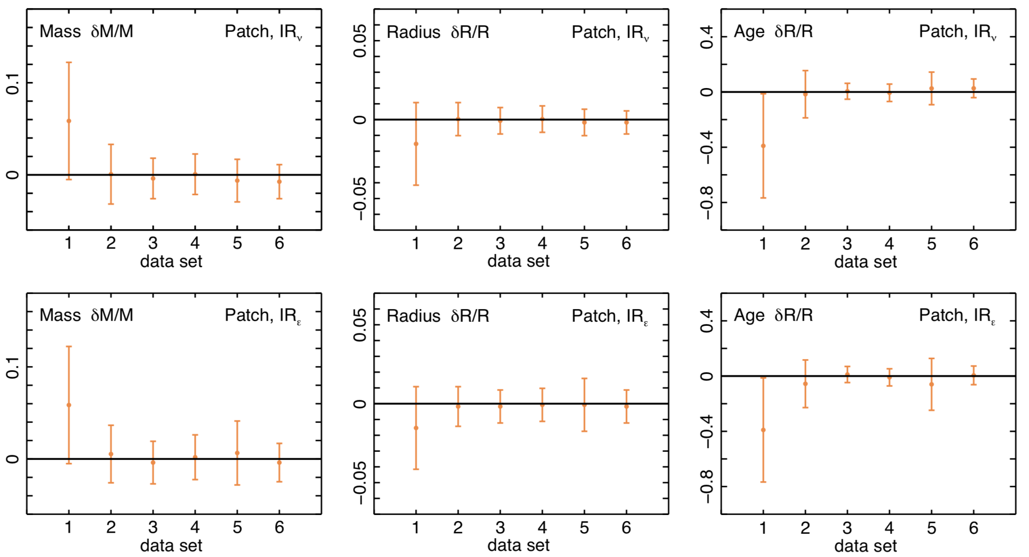
The study of the impact on the inferred stellar properties from changing the observation length and/or the stars’ apparent brightness is beyond the scope of this paper and will be presented in a future work. Here, we address only the impact from changing the set of observed modes and corresponding uncertainties without worrying about the exact underlying cause of those changes. To that end, two exercises were performed, based on the simulations for Patch and Zebedee, the two stars with the same physics as the grid and falling within the grid parameter space. Firstly, we explored the impact on the properties inferred for Patch from decreasing the number of observed modes and the diversity of mode degrees, without modifying the uncertainties in the corresponding mode frequencies. Secondly, we looked at the impact from degrading the quality of the data simulated for Zebedee, with the consequent decrease in the number of observed frequencies and increase in the frequency uncertainties.
Figure 7 shows the results from the first of these exercises, performed with the method IRν, employing a BG-1term correction, and the method IRϵ, both with a 3:3 weight. The seismic data sets considered in the fits are listed in Table 7. The improvement resulting from including any set of seismic data is clear for all three stellar properties. Indeed, an increase in both accuracy and precision is seen when comparing the inferences made by fitting data set 1 (no seismic data) with those made from fits to data sets 2 to 6 (different seismic data combinations). Also striking is the fact that fitting the full set of seismic data or just a small subset of it leads to mass and radius inferences of comparable accuracy and precision. The situation is somewhat different for the age, where the results show that the inclusion of modes in the data set leads to more precise inferences. This is clearly seen by comparing the uncertainty in the age inferred from fitting data sets 3 (including 2 modes of and 2 modes of ) with that inferred from fitting data set 5 (including 8 modes of and 9 modes of ) and is more evident for the surface-independent method.
The data from the two simulations performed for Zebedee in the context of the second exercise are shown in Tables 9 (original data set) and 11 (degraded data set). The number of detected modes decreases from 23 to 7 between the two data sets and the uncertainties in the corresponding frequencies increase by a factor of 3. The impact of these changes is illustrated in Figure 8 and Table 8. The drastic decrease in the number of modes and associated increase in the uncertainties of the detected frequencies, seems to have a relatively modest impact on the precision and accuracy of the mass and radius inferred for the target. For the precision, a maximum of 3.59 per cent and 1.30 per cent is found for the mass and radius, respectively, and for the accuracy, the maximum absolute value of the relative differences, , is 3.46 per cent for the mass and of 1.26 per cent for the radius. Nevertheless, the lack of detection of modes in the degraded data set is found to have a significant impact on the seismic constraining power on the age, in accordance with the findings from the first exercise in this section. Moreover, the impact seems to depend on the inference procedure, being significantly greater in the case of the surface independent method (IRϵ). While for the hounds based on the fitting of individual frequencies we find a for the age of 18 per cent, the relative difference between the true age and the age inferred from the modelling based on the surface independent method is per cent. We note, however, that Zebedee is a relatively young star, having an age of 3 Gyr and a mass comparable to that of the Sun. This young age impacts the measure of the age accuracy and precision since their assessment is based on quantities that depend on the inverse of the true age.
| Set | Comments | |||
|---|---|---|---|---|
| 1 | 0 | 0 | 0 | no frequencies |
| 2 | 2 | 2 | 0 | |
| 3 | 2 | 0 | 2 | |
| 4 | 2 | 2 | 2 | |
| 5 | 8 | 9 | 0 | |
| 6 | 8 | 9 | 6 | full set |
| Massori | Massdeg | Radiusori | Radiusdeg | Ageori | Agedeg | ||
| 1.0165 | 1.0165 | 0.9646 | 0.9646 | 3.085 | 3.085 | ||
| Hounds | |||||||
| Infered value | 1.003(0.027) | 1.010(0.037) | 0.961(0.012) | 0.962(0.013) | 2.99(0.42) | 1.7(1.4) | |
| IRϵ | () | -1.33 | -0.64 | -0.37 | -0.25 | -3.18 | -44.24 |
| -0.50 | -0.18 | -0.30 | -0.20 | -0.23 | -1.00 | ||
| () | 2.66 | 3.59 | 1.24 | 1.29 | 13.71 | 44.14 | |
| Infered value | 1.004(0.027) | 0.993(0.033) | 0.961(0.010) | 0.953(0.013) | 2.97(0.43) | 2.53(1.5) | |
| IRν | () | -1.23 | -2.31 | -0.37 | -1.20 | -3.76 | -18.07 |
| -0.46 | -0.71 | -0.36 | -0.92 | -0.27 | -0.38 | ||
| () | 2.66 | 3.25 | 1.04 | 1.30 | 13.81 | 47.51 | |
| Infered value | 1.008(0.018) | 1.000(0.030) | 0.9627(0.0063) | 0.955(0.011) | 3.01(0.38) | 2.6(1.3) | |
| DR | () | -0.84 | -1.61 | -0.20 | -0.98 | -2.46 | -15.50 |
| -0.47 | -0.55 | -0.31 | -0.85 | -0.20 | -0.38 | ||
| () | 1.77 | 2.95 | 0.65 | 1.16 | 12.38 | 41.16 | |
| Infered value | 0.999(0.028) | 0.981(0.034) | 0.959(0.010) | 0.952(0.011) | 3.02(0.64) | 3.2(1.5) | |
| VA | () | -1.72 | -3.46 | -0.58 | -1.26 | -2.20 | 4.99 |
| -0.62 | -1.04 | -0.57 | -1.12 | -0.11 | 0.10 | ||
| () | 2.79 | 3.33 | 1.01 | 1.12 | 20.86 | 49.09 | |
| () | -1.28 | -2.01 | -0.38 | -0.92 | -2.90 | -18.20 | |
| -0.51 | -0.62 | -0.39 | -0.77 | -0.20 | -0.41 | ||
| () | 1.32 | 2.25 | 0.40 | 1.01 | 2.96 | 25.24 | |
| 0.52 | 0.69 | 0.40 | 0.85 | 0.21 | 0.57 | ||
| () | 2.47 | 3.28 | 0.99 | 1.22 | 15.19 | 45.47 |

8 Impact from the errors on the classical parameters
In this section, we explore the impact on the inferred stellar properties from changing the observational uncertainties on the classical constraints. Two exercises were performed. In the first the 1 uncertainties on [Fe/H], , and were doubled, one at a time, while in the second the observed classical constraints were shifted, along with the original errors, by . The impact on the inferred properties from doubling the uncertainties on the classical constraints was found to be generally negligible for the mass and radius, both in terms of the accuracy and the precision of the results, and smaller, for all three properties, than the impact of shifting the classical constraints by . The differences found when performing these shifts are illustrated in Fig. 9. Here we show, for the first hound (SB; Table 3), a comparison between the properties inferred when considering the original classical observations (Table 2; leftmost point in each cluster of results in Fig 9), and classical observations shifted by , one at the time (following 6 points in each cluster of results).
Inspection of Fig. 9 shows that the impact on the accuracy and precision of the inferred parameters from shifting the classical observations by is generally small, but not negligible, particularly in the case of the age. Using as a reference the relative difference with the true value obtained with the classical observations given in Table 2, (, black in Fig 9), we computed the dispersion of the results for each property and target as before: , where is the number of cases considered. Moreover, we also computed the maximum departure between any given inference and the value inferred in the reference case, . The maximum dispersion is found for Fred, with values of 1.39 per cent, 0.68 per cent, and 6.7 per cent for mass, radius, and age, respectively. The maximum departure from the reference result is also found for Fred. In the case of the mass and age, this maximum is found for shifts in [Fe/H], with values of 2.34 per cent and 11.5 per cent, respectively. For the radius, we find a maximum departure of 0.89 per cent, arising from a shift in .

9 Conclusions
In this work we compared different approaches to the asteroseismic inference of stellar properties based on a pre-computed grid of models and corresponding pulsation properties. The aim was to understand the accuracy and precision that may be expected on the inferred properties when applying state-of-the-art techniques and identify critical aspects of the inference process that may require further development, in light of the preparation for the soon to be launched PLATO mission, from ESA. The study was conducted based on a single grid of models and six main-sequence artificial stars, three of which were generated with the same physics setup as the grid (although one of these has an enrichment ratio outside the range covered by the grid parameter space). The remaining three stars were generated with at least one aspect of the underlying physics differing from the physics adopted for the grid. Five different grid-based inference methods, namely SB, JO, DR, IRϵ and VA, and two variants of these, have been compared. The methods are summarised in appendix B and Table 3.
With regards to the comparison between different grid-based inference methods, our main conclusions can be summarised as follows:
- •
No significant differences were found among the methods elected for comparison with regards to the accuracy of the results, when these are considered in light of the reference values of 15, 2 and 10 per cent in mass, radius and age, respectively. Specifically, considering the 5 targets for which the hounds reported results they could trust (i.e., excluding George), the average relative errors on the inferences made with the 5 different methods varied in the interval 1.61 – 2.61 per cent for the mass, 0.33 – 0.84 per cent for the radius and 5.11 – 6.01 per cent for the age.
- •
Similarly, the differences in precision on the mass among the elected methods was not deemed significant. Considering the same 5 stars, the average precision on mass varied within the interval 1.52 – 2.75 per cent among the 5 methods, in all cases being much smaller than 15 per cent. For the radius, the average precision of the methods was found to vary within the interval 0.58 – 1.23 per cent and for the age within the interval 4.96 – 11.82 per cent. While these differences may seem more significant, we note that to a large extent they result from the relative weight on the classical and seismic constraints adopted by each hound for the elected method. As expected, methods applying a 3:1 weight generally have larger error bars than those applying a 3:3 weight (where 3:1/3:3 indicates that the full set of frequencies is given the same weight as one/three global constraints, respectively; cf. Sections 3.1 and 6). However, this weight is not intrinsic to the method (in the sense that different weights can be adopted with the same method). Thus, the differences seen in the precision of the inferred properties do not translate into a fundamental difference in the potential precision of the methods themselves. In addition, the significant average age precision of 4.96 per cent found with the method by the hound JO resulted in part from neglecting the perturbation of the frequencies in the MC simulations, as noted in Section 3.2. When considering the same weight (Fig. 5) the precision of different methods on age was found to be similar. For the radius, the method employed by DR seems to be the most precise and that by IRϵ the least precise, with the error bars on the latter found to be up to a factor of 2 larger than those on the former.
Concerning the impact of the ad hoc choices that may be involved in the inference procedures, such as those associated with the surface corrections and the relative weight set on the classical and seismic constraints, we reached the following conclusions:
- •
If surface corrections are not added to the model frequencies when these are used directly in the fits, the relative differences between the inferred and true values of the stellar properties are very significant. For the method by DR, on which the surface corrections tests were based, the relative differences were found to be as large as 7, 3 and 35 per cent for mass, radius and age, respectively, in the absence of a surface correction. The inclusion of a BG-2term surface correction in this method reduces the maximum of the relative differences on mass, radius and age to 2.36, 0.9 and 11.25 per cent. Still, the choice of the prescription for the surface corrections was found to impact the results, leading to a maximum dispersion on the inferences of 1.9, 1.0 and 6.8 per cent in mass, radius and age, respectively. While these values of the dispersion are smaller than the reference values, they are by no means negligible in the case of the radius and age. Thus, this result calls for an improvement of the modelling of the surface layers of stars, both in what concerns the structure and the pulsations (Mosumgaard et al. 2020; Belkacem et al. 2021; Jørgensen et al. 2021).
- •
Given a set of observations, the adoption of a weight in the fitting procedure aimed at decreasing the relative impact of the seismic data with regards to the classical data is equivalent to an ad hoc inflation of the errors on the frequencies. To be statistically sound, the inference method to be used in the PLATO pipeline should instead give each observation the same weight (our 3:N case). However, our results show that when the targets do not share the physics setup of the grid, as will generally happen for real stars, the properties inferred with a 3:N approach can be many sigma away from the true property values. This is mostly related to the fact that a 3:N approach leads to significantly smaller uncertainties on the inferred properties when the grid does not contain a reasonable sample of comparably good models around the inferred solution. This result points to an urgent need to thoroughly characterise the systematic errors incurred on the inferred stellar properties when performing inferences based on a grid similar to the one to be adopted by the PLATO mission. These systematic errors, resulting from fixing a given set of options concerning the physics of the grid, need to be considered along with the formal errors derived from the application of the inference procedure, in order to provide robust uncertainties on the inferred properties of PLATO stars. In some cases, our results also show a non-negligible change in accuracy when comparing the 3:3 and 3:N weights, both for methods with and without interpolation between grid models. Further studies should be pursued to understand these differences, and in particular, to investigate whether they are connected to the grid resolution.
Finally, we have tested the impact of degrading the classical and seismic data. With regards to these tests our conclusions were as follows:
- •
Concerning the classical data, the most significant impact was found when shifting the central values. Specifically, when changing , and [Fe/H] by 1 , one at a time, the dispersion in the inferred relative differences reached up to 1.39, 0.68 and 6.7 per cent in mass, radius and age, respectively. Moreover, the maximum difference between any two mass or age inferences was found when shifting the value of [Fe/H] and reached 2.34 per cent for mass and 11.5 per cent for age. For the radius the maximum difference was found when shifting and did not exceed 1 per cent. These results highlight the importance of determining the classical parameters to a high precision and accuracy, particularly when considering the impact they have when inferring the stellar age.
- •
Concerning the seismic data, our results show that the detection of only a small number of oscillation frequencies may be enough to set stringent constraints on the stellar mass and radius. While that seems to be true also for the age, in this case we found that the precision of the inferences depends more strongly on the combination of mode degrees available for the fit, with the results becoming more precise when at least one mode is detected. When in addition to reducing the number of modes and eliminating the modes of degree , the uncertainties in the mode frequencies are increased, the inference of a precise and accurate age starts to be compromised. It is, therefore, important to investigate thoroughly the case of stars in the regime where seismic data becomes limited and the inference approach eventually changes from fitting individual frequencies or phases to fitting global seismic constraints.
It is worth noting that the conclusions summarised here are based on the study of targets whose physics is relatively standard. However, even in the case of low mass stars, some non-standard processes may have a significant evolutionary impact. An example are macroscopic and microscopic processes leading to chemical transport in radiative regions inside stars (see Aerts 2021, for a review), that, together, dictate the observed surface abundances at a given time in evolution. As illustrated by our study of Gerald, considerable biases in mass and age can result from not accounting for atomic diffusion. In stars slightly more massive than Gerald (and in particular for F stars), the contribution of radiative accelerations to atomic diffusion becomes non-negligible (Deal et al. 2018) and even in relatively slow rotators, rotationally-induced mixing may become an important effect counteracting atomic diffusion (Deal et al. 2020). These effects, neglected in standard models, may lead to additional biases in the inferred stellar properties, not considered in the present work. This emphasises the need to continue developing a new generation of stellar evolution codes and to acquire data on pulsating stars that may help constrain further these aspects of the physics.
The results presented in this work provide guidance for the development of the PLATO pipeline where it concerns the inference of the properties of stars with seismic data and the characterisation of the associated exoplanetary systems. Moreover, the work identifies additional paths of research that should be pursued in order to achieve the PLATO goals and optimise the science return of the mission.
Acknowledgements
This work presents results from the European Space Agency (ESA) space mission PLATO. The PLATO payload, the PLATO Ground Segment and PLATO data processing are joint developments of ESA and the PLATO Mission Consortium (PMC). Funding for the PMC is provided at national levels, in particular by countries participating in the PLATO Multilateral Agreement (Austria, Belgium, Czech Republic, Denmark, France, Germany, Italy, Netherlands, Portugal, Spain, Sweden, Switzerland, Norway, and United Kingdom) and institutions from Brazil. Members of the PLATO Consortium can be found at https://platomission.com/. The ESA PLATO mission website is https://www.cosmos.esa.int/plato. We thank the teams working for PLATO for all their work. MSC acknowledges the support by FCT/MCTES through the research grants UIDB/04434/2020, UIDP/04434/2020 and PTDC/FIS-AST/30389/2017, and by FEDER through COMPETE2020 (grant: POCI-01-0145-FEDER-030389). MSC and TC are supported by national funds through FCT in the form of work contracts (CEECIND/02619/2017 and CEECIND/00476/2018, respectively). JLR acknowledges support from the Carlsberg Foundation (grant agreement CF19-0649). Funding for the Stellar Astrophysics Centre is provided by The Danish National Research Foundation (Grant DNRF106). This article made use of AIMS, a software for fitting stellar pulsation data, developed in the context of the SPACEINN network, funded by the European Commission’s Seventh Framework Programme. BN acknowledges funding from the Alexander von Humboldt Foundation and "Branco Weiss fellowship – Science in Society" through the SEISMIC stellar interior physics group. DRR, M-JG, KB, RMO acknowledge the support of the French space agency (CNES). A.S. acknowledge support from the European Research Council Consolidator Grant funding scheme (project ASTEROCHRONOMETRY, G.A. n. 772293).
Data Availability
References
- Aerts (2021) Aerts C., 2021, Reviews of Modern Physics, 93, 015001
- Aguirre Børsen-Koch et al. (2021) Aguirre Børsen-Koch V., et al., 2021, arXiv e-prints, p. arXiv:2109.14622
- Angulo et al. (1999) Angulo C., et al., 1999, Nuclear Physics A, 656, 3
- Badnell et al. (2005) Badnell N. R., Bautista M. A., Butler K., Delahaye F., Mendoza C., Palmeri P., Zeippen C. J., Seaton M. J., 2005, MNRAS, 360, 458
- Ball & Gizon (2014) Ball W. H., Gizon L., 2014, A&A, 568, A123
- Belkacem et al. (2021) Belkacem K., Kupka F., Philidet J., Samadi R., 2021, A&A, 646, L5
- Broomhall et al. (2009) Broomhall A. M., Chaplin W. J., Davies G. R., Elsworth Y., Fletcher S. T., Hale S. J., Miller B., New R., 2009, MNRAS, 396, L100
- Bruntt et al. (2010) Bruntt H., et al., 2010, MNRAS, 405, 1907
- Chaplin et al. (2014) Chaplin W. J., et al., 2014, ApJS, 210, 1
- Christensen-Dalsgaard (2008) Christensen-Dalsgaard J., 2008, Ap&SS, 316, 13
- Christensen-Dalsgaard et al. (1996) Christensen-Dalsgaard J., et al., 1996, Science, 272, 1286
- Cox & Giuli (1968) Cox J., Giuli R., 1968, Principles of Stellar Structure: Physical principles. No. v. 1 in Principles of Stellar Structure, Gordon and Breach, http://books.google.co.in/books?id=TdhEAAAAIAAJ
- Cunha (2020) Cunha M. S., 2020, Astrophysics and Space Science Proceedings, 57, 185
- Cunha et al. (2003) Cunha M. S., Fernandes J. M. M. B., Monteiro M. J. P. F. G., 2003, MNRAS, 343, 831
- Davies et al. (2014) Davies G. R., Broomhall A. M., Chaplin W. J., Elsworth Y., Hale S. J., 2014, MNRAS, 439, 2025
- Deal et al. (2018) Deal M., Alecian G., Lebreton Y., Goupil M. J., Marques J. P., LeBlanc F., Morel P., Pichon B., 2018, A&A, 618, A10
- Deal et al. (2020) Deal M., Goupil M. J., Marques J. P., Reese D. R., Lebreton Y., 2020, A&A, 633, A23
- Eddington (1926) Eddington A. S., 1926, The Internal Constitution of the Stars. Cambridge: Cambridge Univ. Press
- Ferguson et al. (2005) Ferguson J. W., Alexander D. R., Allard F., Barman T., Bodnarik J. G., Hauschildt P. H., Heffner-Wong A., Tamanai A., 2005, ApJ, 623, 585
- Gilliland et al. (2010) Gilliland R. L., et al., 2010, PASP, 122, 131
- Gough (1990) Gough D. O., 1990, in Osaki Y., Shibahashi H., eds, Lecture Notes in Physics, Berlin Springer Verlag Vol. 367, Progress of Seismology of the Sun and Stars. p. 283, doi:10.1007/3-540-53091-6
- Grevesse & Sauval (1998) Grevesse N., Sauval A. J., 1998, Space Sci. Rev., 85, 161
- Halbwachs et al. (2020) Halbwachs J. L., et al., 2020, MNRAS, 496, 1355
- Hastings (1970) Hastings W. K., 1970, Biometrika, 57, 97
- Herwig (2000) Herwig F., 2000, A&A, 360, 952
- Huber et al. (2012) Huber D., et al., 2012, ApJ, 760, 32
- Imbriani et al. (2005) Imbriani G., et al., 2005, European Physical Journal A, 25, 455
- Jørgensen et al. (2021) Jørgensen A. C. S., et al., 2021, MNRAS, 500, 4277
- Kjeldsen et al. (2008) Kjeldsen H., Bedding T. R., Christensen-Dalsgaard J., 2008, ApJ, 683, L175
- Kunz et al. (2002) Kunz R., Fey M., Jaeger M., Mayer A., Hammer J. W., Staudt G., Harissopulos S., Paradellis T., 2002, ApJ, 567, 643
- Lebreton & Goupil (2014) Lebreton Y., Goupil M. J., 2014, A&A, 569, A21
- Metropolis et al. (1953) Metropolis N., Rosenbluth A. W., Rosenbluth M. N., Teller A. H., Teller E., 1953, The journal of chemical physics, 21, 1087
- Miglio et al. (2017) Miglio A., et al., 2017, Astronomische Nachrichten, 338, 644
- Mosumgaard et al. (2020) Mosumgaard J. R., Jørgensen A. C. S., Weiss A., Silva Aguirre V., Christensen-Dalsgaard J., 2020, MNRAS, 491, 1160
- Nsamba et al. (2018) Nsamba B., Campante T. L., Monteiro M. J. P. F. G., Cunha M. S., Rendle B. M., Reese D. R., Verma K., 2018, MNRAS, 477, 5052
- Nsamba et al. (2021) Nsamba B., et al., 2021, MNRAS, 500, 54
- Ong & Basu (2019) Ong J. M. J., Basu S., 2019, ApJ, 885, 26
- Ong et al. (2021) Ong J. M. J., Basu S., McKeever J. M., 2021, ApJ, 906, 54
- Paxton et al. (2011) Paxton B., Bildsten L., Dotter A., Herwig F., Lesaffre P., Timmes F., 2011, ApJS, 192, 3
- Paxton et al. (2013) Paxton B., et al., 2013, ApJS, 208, 4
- Paxton et al. (2015) Paxton B., et al., 2015, ApJS, 220, 15
- Paxton et al. (2018) Paxton B., et al., 2018, ApJS, 234, 34
- Rauer et al. (2014) Rauer H., et al., 2014, Experimental Astronomy, 38, 249
- Reese et al. (2016) Reese D. R., et al., 2016, A&A, 592, A14
- Rendle et al. (2019) Rendle B. M., et al., 2019, MNRAS, 484, 771
- Rogers & Nayfonov (2002) Rogers F. J., Nayfonov A., 2002, ApJ, 576, 1064
- Roxburgh (2015) Roxburgh I. W., 2015, A&A, 574, A45
- Roxburgh (2016) Roxburgh I. W., 2016, A&A, 585, A63
- Roxburgh & Vorontsov (2003) Roxburgh I. W., Vorontsov S. V., 2003, A&A, 411, 215
- Sahlholdt & Silva Aguirre (2018) Sahlholdt C. L., Silva Aguirre V., 2018, MNRAS, 481, L125
- Santos & Buchhave (2018) Santos N. C., Buchhave L. A., 2018, Accurate Stellar Parameters for Radial Velocity Surveys. p. 181, doi:10.1007/978-3-319-55333-7_181
- Seaton (2005) Seaton M. J., 2005, MNRAS, 362, L1
- Serenelli et al. (2021) Serenelli A., et al., 2021, A&ARv, 29, 4
- Silva Aguirre et al. (2015) Silva Aguirre V., et al., 2015, MNRAS, 452, 2127
- Silva Aguirre et al. (2017) Silva Aguirre V., et al., 2017, ApJ, 835, 173
- Sobol (1967) Sobol I. M., 1967, USSR Comp. Math. and Math. Phys., 7, 4
- Sonoi et al. (2015) Sonoi T., Samadi R., Belkacem K., Ludwig H. G., Caffau E., Mosser B., 2015, A&A, 583, A112
- Stello et al. (2009) Stello D., et al., 2009, ApJ, 700, 1589
- Thoul et al. (1994) Thoul A. A., Bahcall J. N., Loeb A., 1994, ApJ, 421, 828
- Torres et al. (2010) Torres G., Andersen J., Giménez A., 2010, A&ARv, 18, 67
- Verma et al. (2017) Verma K., Raodeo K., Antia H. M., Mazumdar A., Basu S., Lund M. N., Silva Aguirre V., 2017, ApJ, 837, 47
- Vernazza et al. (1981) Vernazza J. E., Avrett E. H., Loeser R., 1981, ApJS, 45, 635
- Winn & Fabrycky (2015) Winn J. N., Fabrycky D. C., 2015, ARA&A, 53, 409
Appendix A Data sets produced by the Hares
Tables 9-10 list the properties of the individual modes simulated for the targets in Table 1, specifically: the mode degree, , the radial order, , the true mode frequency value, , the simulated frequency, , and its uncertainty, . Table 11 lists the set of degraded observations simulated for Zebedee for the exercise in Section 7.
| Patch | ||||
|---|---|---|---|---|
| (Hz) | (Hz) | (Hz) | ||
| 0 | 16 | 2343.51 | 2343.23 | 0.31 |
| 0 | 17 | 2475.44 | 2475.35 | 0.20 |
| 0 | 18 | 2608.14 | 2608.24 | 0.16 |
| 0 | 19 | 2741.55 | 2741.40 | 0.16 |
| 0 | 20 | 2874.71 | 2874.55 | 0.18 |
| 0 | 21 | 3007.94 | 3008.00 | 0.23 |
| 0 | 22 | 3141.48 | 3141.43 | 0.38 |
| 0 | 23 | 3275.42 | 3274.02 | 0.73 |
| 1 | 15 | 2272.92 | 2273.13 | 0.36 |
| 1 | 16 | 2405.01 | 2404.83 | 0.21 |
| 1 | 17 | 2537.98 | 2537.87 | 0.15 |
| 1 | 18 | 2671.46 | 2671.57 | 0.13 |
| 1 | 19 | 2805.19 | 2805.21 | 0.14 |
| 1 | 20 | 2938.88 | 2939.08 | 0.17 |
| 1 | 21 | 3072.45 | 3071.81 | 0.25 |
| 1 | 22 | 3206.60 | 3206.53 | 0.43 |
| 1 | 23 | 3341.21 | 3340.91 | 0.93 |
| 2 | 16 | 2468.27 | 2468.04 | 0.33 |
| 2 | 17 | 2601.55 | 2601.61 | 0.26 |
| 2 | 18 | 2735.51 | 2735.41 | 0.25 |
| 2 | 19 | 2869.20 | 2869.31 | 0.28 |
| 2 | 20 | 3002.96 | 3002.43 | 0.37 |
| 2 | 21 | 3136.95 | 3136.34 | 0.59 |
| - | - | - | - | - |
| - | - | - | - | - |
| - | - | - | - | - |
| - | - | - | - | - |
| - | - | - | - | - |
| - | - | - | - | - |
| - | - | - | - | - |
| - | - | - | - | - |
| - | - | - | - | - |
| Zebedee | ||||
|---|---|---|---|---|
| (Hz) | (Hz) | (Hz) | ||
| 0 | 18 | 2795.03 | 2794.98 | 0.29 |
| 0 | 19 | 2936.71 | 2936.89 | 0.19 |
| 0 | 20 | 3079.03 | 3078.92 | 0.16 |
| 0 | 21 | 3221.73 | 3221.60 | 0.16 |
| 0 | 22 | 3364.06 | 3364.43 | 0.20 |
| 0 | 23 | 3506.45 | 3506.28 | 0.30 |
| 0 | 24 | 3649.01 | 3647.87 | 0.54 |
| 0 | 25 | 3791.98 | 3789.75 | 1.14 |
| 1 | 17 | 2720.28 | 2720.07 | 0.34 |
| 1 | 18 | 2861.65 | 2861.36 | 0.20 |
| 1 | 19 | 3003.99 | 3004.19 | 0.14 |
| 1 | 20 | 3146.59 | 3146.30 | 0.13 |
| 1 | 21 | 3289.29 | 3289.14 | 0.15 |
| 1 | 22 | 3431.82 | 3431.59 | 0.20 |
| 1 | 23 | 3574.24 | 3574.49 | 0.33 |
| 1 | 24 | 3717.20 | 3718.28 | 0.64 |
| 1 | 25 | 3860.49 | 3857.98 | 1.48 |
| 2 | 18 | 2924.95 | 2924.71 | 0.31 |
| 2 | 19 | 3067.60 | 3067.29 | 0.26 |
| 2 | 20 | 3210.61 | 3210.91 | 0.26 |
| 2 | 21 | 3353.27 | 3353.16 | 0.32 |
| 2 | 22 | 3495.98 | 3496.49 | 0.47 |
| 2 | 23 | 3638.78 | 3637.81 | 0.82 |
| - | - | - | - | - |
| - | - | - | - | - |
| - | - | - | - | - |
| - | - | - | - | - |
| - | - | - | - | - |
| - | - | - | - | - |
| - | - | - | - | - |
| - | - | - | - | - |
| - | - | - | - | - |
| Fred | ||||
|---|---|---|---|---|
| (Hz) | (Hz) | (Hz) | ||
| 0 | 13 | 971.45 | 971.05 | 0.94 |
| 0 | 14 | 1037.84 | 1036.91 | 0.77 |
| 0 | 15 | 1104.53 | 1105.40 | 0.66 |
| 0 | 16 | 1172.63 | 1171.94 | 0.59 |
| 0 | 17 | 1242.10 | 1242.45 | 0.54 |
| 0 | 18 | 1312.39 | 1312.31 | 0.52 |
| 0 | 19 | 1382.37 | 1382.99 | 0.53 |
| 0 | 20 | 1451.27 | 1451.34 | 0.56 |
| 0 | 21 | 1519.49 | 1518.40 | 0.63 |
| 0 | 22 | 1587.67 | 1587.10 | 0.76 |
| 0 | 23 | 1656.26 | 1656.52 | 1.00 |
| 0 | 24 | 1725.79 | 1728.67 | 1.47 |
| 1 | 12 | 934.62 | 935.19 | 0.91 |
| 1 | 13 | 1001.68 | 1001.87 | 0.74 |
| 1 | 14 | 1067.86 | 1067.13 | 0.62 |
| 1 | 15 | 1135.10 | 1133.87 | 0.53 |
| 1 | 16 | 1203.81 | 1202.85 | 0.48 |
| 1 | 17 | 1273.76 | 1274.52 | 0.45 |
| 1 | 18 | 1344.08 | 1344.35 | 0.44 |
| 1 | 19 | 1413.64 | 1413.34 | 0.46 |
| 1 | 20 | 1482.22 | 1482.53 | 0.50 |
| 1 | 21 | 1550.46 | 1550.98 | 0.58 |
| 1 | 22 | 1618.89 | 1618.46 | 0.72 |
| 1 | 23 | 1688.00 | 1687.72 | 1.00 |
| 2 | 14 | 1099.01 | 1097.51 | 1.07 |
| 2 | 15 | 1166.93 | 1167.08 | 0.95 |
| 2 | 16 | 1236.26 | 1235.29 | 0.87 |
| 2 | 17 | 1306.51 | 1307.35 | 0.84 |
| 2 | 18 | 1376.56 | 1375.87 | 0.84 |
| 2 | 19 | 1445.59 | 1445.21 | 0.89 |
| 2 | 20 | 1513.89 | 1514.92 | 0.99 |
| 2 | 21 | 1582.14 | 1582.95 | 1.19 |
| Gerald | ||||
|---|---|---|---|---|
| (Hz) | (Hz) | (Hz) | ||
| 0 | 15 | 1706.25 | 1706.47 | 0.24 |
| 0 | 16 | 1807.84 | 1807.47 | 0.15 |
| 0 | 17 | 1910.09 | 1910.07 | 0.11 |
| 0 | 18 | 2013.33 | 2013.11 | 0.10 |
| 0 | 19 | 2116.36 | 2116.48 | 0.11 |
| 0 | 20 | 2219.24 | 2219.29 | 0.12 |
| 0 | 21 | 2322.51 | 2322.75 | 0.16 |
| 0 | 22 | 2425.98 | 2425.89 | 0.24 |
| 0 | 23 | 2529.90 | 2529.59 | 0.46 |
| 1 | 14 | 1649.67 | 1650.16 | 0.29 |
| 1 | 15 | 1751.59 | 1751.46 | 0.16 |
| 1 | 16 | 1854.03 | 1854.06 | 0.11 |
| 1 | 17 | 1957.00 | 1957.02 | 0.09 |
| 1 | 18 | 2060.39 | 2060.37 | 0.09 |
| 1 | 19 | 2163.93 | 2164.05 | 0.09 |
| 1 | 20 | 2267.15 | 2267.16 | 0.11 |
| 1 | 21 | 2370.70 | 2370.64 | 0.16 |
| 1 | 22 | 2474.93 | 2474.73 | 0.27 |
| 1 | 23 | 2579.29 | 2579.56 | 0.58 |
| 2 | 15 | 1801.62 | 1801.50 | 0.24 |
| 2 | 16 | 1904.23 | 1904.16 | 0.19 |
| 2 | 17 | 2007.81 | 2008.10 | 0.17 |
| 2 | 18 | 2111.20 | 2111.20 | 0.17 |
| 2 | 19 | 2214.50 | 2214.53 | 0.19 |
| 2 | 20 | 2318.14 | 2318.34 | 0.25 |
| 2 | 21 | 2421.96 | 2421.70 | 0.38 |
| 2 | 22 | 2526.28 | 2527.13 | 0.72 |
| - | - | - | - | - |
| - | - | - | - | - |
| - | - | - | - | - |
| - | - | - | - | - |
| - | - | - | - | - |
| - | - | - | - | - |
| - | - | - | - | - |
| - | - | - | - | - |
| Zippy | ||||
|---|---|---|---|---|
| (Hz) | (Hz) | (Hz) | ||
| 0 | 13 | 1238.22 | 1239.08 | 0.53 |
| 0 | 14 | 1324.78 | 1324.53 | 0.37 |
| 0 | 15 | 1410.83 | 1411.18 | 0.28 |
| 0 | 16 | 1495.27 | 1494.80 | 0.23 |
| 0 | 17 | 1579.81 | 1580.39 | 0.21 |
| 0 | 18 | 1665.40 | 1665.50 | 0.20 |
| 0 | 19 | 1752.11 | 1752.00 | 0.21 |
| 0 | 20 | 1838.94 | 1838.99 | 0.24 |
| 0 | 21 | 1925.46 | 1925.26 | 0.30 |
| 0 | 22 | 2011.72 | 2012.07 | 0.45 |
| 0 | 23 | 2098.20 | 2098.64 | 0.78 |
| 1 | 12 | 1189.99 | 1189.87 | 0.59 |
| 1 | 13 | 1276.40 | 1276.66 | 0.38 |
| 1 | 14 | 1363.08 | 1362.97 | 0.27 |
| 1 | 15 | 1448.41 | 1448.50 | 0.22 |
| 1 | 16 | 1532.90 | 1533.33 | 0.19 |
| 1 | 17 | 1617.90 | 1617.86 | 0.17 |
| 1 | 18 | 1704.40 | 1704.86 | 0.17 |
| 1 | 19 | 1791.40 | 1791.68 | 0.19 |
| 1 | 20 | 1878.46 | 1878.61 | 0.22 |
| 1 | 21 | 1965.00 | 1964.84 | 0.30 |
| 1 | 22 | 2051.67 | 2051.53 | 0.48 |
| 1 | 23 | 2138.62 | 2139.27 | 0.91 |
| 2 | 13 | 1318.06 | 1318.56 | 0.60 |
| 2 | 14 | 1404.34 | 1404.56 | 0.45 |
| 2 | 15 | 1488.97 | 1489.17 | 0.37 |
| 2 | 16 | 1573.63 | 1574.06 | 0.33 |
| 2 | 17 | 1659.29 | 1659.30 | 0.32 |
| 2 | 18 | 1746.20 | 1746.07 | 0.33 |
| 2 | 19 | 1833.26 | 1832.56 | 0.38 |
| 2 | 20 | 1920.09 | 1920.62 | 0.48 |
| 2 | 21 | 2006.63 | 2007.57 | 0.70 |
| 2 | 22 | 2093.40 | 2093.48 | 1.21 |
| - | - | - | - | - |
| - | - | - | - | - |
| George | ||||
|---|---|---|---|---|
| (Hz) | (Hz) | (Hz) | ||
| 0 | 13 | 986.72 | 986.52 | 0.44 |
| 0 | 14 | 1055.70 | 1055.59 | 0.28 |
| 0 | 15 | 1125.65 | 1125.73 | 0.21 |
| 0 | 16 | 1194.98 | 1194.94 | 0.17 |
| 0 | 17 | 1263.30 | 1263.60 | 0.15 |
| 0 | 18 | 1331.12 | 1330.98 | 0.14 |
| 0 | 19 | 1399.92 | 1399.97 | 0.15 |
| 0 | 20 | 1469.69 | 1469.46 | 0.16 |
| 0 | 21 | 1540.26 | 1540.18 | 0.20 |
| 0 | 22 | 1610.67 | 1610.93 | 0.28 |
| 0 | 23 | 1680.94 | 1680.96 | 0.44 |
| 0 | 24 | 1750.73 | 1750.91 | 0.85 |
| 1 | 12 | 951.51 | 951.58 | 0.50 |
| 1 | 13 | 1019.70 | 1019.58 | 0.30 |
| 1 | 14 | 1089.90 | 1089.83 | 0.20 |
| 1 | 15 | 1159.98 | 1159.97 | 0.16 |
| 1 | 16 | 1229.28 | 1229.26 | 0.14 |
| 1 | 17 | 1297.42 | 1297.56 | 0.13 |
| 1 | 18 | 1366.01 | 1365.98 | 0.12 |
| 1 | 19 | 1435.54 | 1435.38 | 0.13 |
| 1 | 20 | 1506.05 | 1505.87 | 0.15 |
| 1 | 21 | 1576.72 | 1576.79 | 0.20 |
| 1 | 22 | 1647.11 | 1647.16 | 0.29 |
| 1 | 23 | 1717.08 | 1717.01 | 0.51 |
| 1 | 24 | 1786.73 | 1787.51 | 1.09 |
| 2 | 13 | 1051.31 | 1051.04 | 0.47 |
| 2 | 14 | 1121.39 | 1120.90 | 0.34 |
| 2 | 15 | 1190.88 | 1190.94 | 0.27 |
| 2 | 16 | 1259.38 | 1259.06 | 0.24 |
| 2 | 17 | 1327.27 | 1327.30 | 0.23 |
| 2 | 18 | 1396.12 | 1395.78 | 0.24 |
| 2 | 19 | 1465.91 | 1466.19 | 0.26 |
| 2 | 20 | 1536.54 | 1536.09 | 0.32 |
| 2 | 21 | 1607.01 | 1606.78 | 0.43 |
| 2 | 22 | 1677.32 | 1676.46 | 0.69 |
| = 1.00 0.03 | |||
|---|---|---|---|
| = 5887 85 K | |||
| [Fe/H] = -0.03 0.09 dex | |||
| = 3260 167 Hz | |||
| = 143.1 2.8 Hz | |||
| (Hz) | (Hz) | ||
| 0 | 21 | 3223.09 | 0.48 |
| 0 | 22 | 3364.38 | 0.63 |
| 1 | 19 | 3004.18 | 0.44 |
| 1 | 20 | 3147.48 | 0.39 |
| 1 | 21 | 3289.17 | 0.45 |
| 1 | 22 | 3433.58 | 0.65 |
| 1 | 23 | 3576.01 | 1.17 |
Appendix B Methods employed by the Hounds
B.1 SB: The grid method
This method used the provided grid as-is, without any interpolation. The first step in the analysis of each target was to select the subset of models that lay within of , , , luminosity and [Fe/H] of each star. While a -cut is generally sufficient, the cut allowed us to use the same set of models for the tests where the spectroscopic parameters were shifted by 1.
The frequencies of each of the selected models were corrected for surface effects using the Ball & Gizon 2014 two-term correction. The parameters for the correction were determined using radial modes and then applied to all modes. The corrected frequencies were then used to calculate the per degree of freedom, which we call , for each model. This is defined as:
| (9) |
where is the uncertainty on the frequency of the target, and the sum is over all observed frequencies. This is then used to calculate a likelihood
| (10) |
being the normalisation constant.
The surface term correction does not take into account the fact that the frequency difference between the model and the star is expected to be smaller at low frequencies than at high frequencies. There are many models in the grid that are different enough from the star that the high-frequency modes match but the low-frequency modes do not. Additionally, contrary to the expectations, the low-frequency modes of these models have lower frequencies than that of the star. To ensure that these models are given a lower weight than others, we also calculated the value for the 2 lowest uncorrected model frequencies for all available degrees. We divide this by 10000 to reduce this term’s contribution to the likelihood, call it , and calculate a weight that is defined as
| (11) |
where W is a normalisation constant. Since is normalised such that its sum over all models is 1, the division by 10000 results in a gentle down selection.
As with the corrected frequencies, we calculate likelihoods for , luminosity and [Fe/H]. For example, the likelihood for effective temperature was defined as
| (12) |
with
| (13) |
where is the uncertainty on the effective temperature, and the normalisation constant. We define the likelihoods for [Fe/H] and in a similar manner.
The total likelihood for each model is then
| (14) |
The means of the marginalised likelihoods of the ensemble of models were used to determine the parameters of the star, after converting them to a probability density by normalising the likelihood by the prior distribution of the property.
B.2 JO: Grid Monte Carlo
We use the same Monte-Carlo grid search procedure as in Ong et al. 2021, but with a different set of penalty functions. For each model, an overall cost function is computed as the sum of the following contributions:
- •
, where are global quantities: we have used the classical spectroscopic constraints, as well as and (Ong & Basu 2019, the radial mode phase offset at , in the sense of).
- •
, being the reduced- penalty function from applying the surface correction of Ball & Gizon 2014. The parameters are fitted against only the radial modes, and then the cost function is computed from applying the correction to all mode frequencies.
- •
, which is the reduced function of the -matching algorithm described in Roxburgh 2016 — cf. their eq. 12 and discussion in §B.4.
- •
: under the ansatz that the surface term affects higher-order modes more than it does low-order ones, we construct a quantity , summing over only the lowest-frequency radial modes. is an asymmetric penalty function satisfying
(15) for some constant . This is to penalise surface corrections which modify low-frequency modes too much, as well as to ensure that the sense of the surface term is the same as seen in the case of the solar surface term. For this exercise we have used . We moreover downweighted this term by a factor of , to ensure that the only function it serves is that of regularisation.
For each model , we treat the quantity , normalised to sum to 1 over all models in the grid, as a likelihood weight function. Here is the grid’s sampling density function, which may not be uniform, and is not assumed to be known in advance. We estimate using a kernel density estimate applied to the grid parameters (including model ages). We then compute the weighted mean of each of the output quantities with respect to these likelihood weights , summing over all models in the grid. This corresponds to taking the posterior means of the desired output properties, under the assumption of uniform priors on the model parameters.
We repeat the same procedure, perturbing each of the spectroscopic and average seismic inputs by a normally-distributed random amount with variance given by the observational errors. Unless otherwise indicated, we do not perturb the frequencies, since evaluating the cost terms associated with individual mode frequencies is extremely expensive. We collect these posterior means associated with each realisation, over realisations. The posterior means define a mapping , where are the supplied observations, and the desired output properties (e.g., mass, radius, etc). By perturbing the input observations in this manner, we directly propagate "input" probability distributions on to "output" probability distributions on under the action of the map . We report the marginalised medians and quantiles as our estimates for the values and uncertainties of the output parameters with respect to these output probability distributions.
B.3 DR: AIMS
The Asteroseismic Inference on a Massive Scale (AIMS) code takes in a grid of models and applies a Markov Chain Monte Carlo (MCMC) approach to fitting a given set of classic and seismic constraints. In order to allow the MCMC approach to explore the parameter space more freely, AIMS carries out interpolation within the input grid of models using a triangulation (or tessellation) of the parameter space between the evolutionary tracks, and linear interpolation along the tracks. This gives it a great degree of flexibility in terms of the location of the evolutionary tracks in parameter space. The interpolation is applied both to model properties such as mass, radius, and age, and to the pulsation frequencies. This then provides all of the necessary information to calculate the priors and likelihood function which intervene in the probability calculations. Once the MCMC run is completed, a representative sample of models is obtained from which it is possible to calculate posterior probability distributions for the models properties, as well as statistical averages, standard deviations, correlations, and various percentiles. For more details on the AIMS code, we refer the reader to Rendle et al. 2019 as well as to the AIMS documentation33 3 The latest version of AIMS is available at: https://gitlab.com/sasp/aims.
In the present hare-and-hounds exercise, AIMS was used to fit the hares using a variety of different settings. In terms of surface corrections, the approaches by Kjeldsen et al. 2008, Ball & Gizon 2014, and Sonoi et al. 2015 were used. In each case, variants with one and two free parameters were used (in particular, the second parameter for the Kjeldsen et al. 2008 surface correction is the exponent and that of the Sonoi et al. 2015 correction is the exponent, both of which are fitted non-linearly with the MCMC approach). Runs without surface corrections were also carried. A cutoff on classic constraints was applied, except when applying the two-term Ball & Gizon 2014 surface correction where various cutoffs where applied: , , , . With the exception of George in the specific case of a cutoff, the differences in the results for different cutoffs were found to be negligible. Thus, only the cutoff results are shown. In all cases we used uniform priors on the relevant ranges of the parameters. In the case of the age, a uniform prior over the interval [0, 13.8] Gyr was considered. Various weights on classic and seismic constraints were adopted for the runs, namely 3:3, 3:N, and in a few cases 3:1. The constraint on was not included but it is possible to include it.
B.4 IRϵ: surface independent
Epsilon matching is a “surface layer independent” model comparison algorithm which subtracts the contribution of the outer layers of the stars from a combination of their frequencies. The epsilon matching algorithm used here is described in detail in Roxburgh 2016.
In short, the (adiabatic) oscillation frequencies of a star can be expressed in terms of epsilons, , as
where is an estimate of the large separation. Moreover, the can be expressed in terms of an -dependent inner phase shift determined by the inner structure of the star, , and an -independent outer phase shift, , determined by the structure of the outer layers, such that .
The algorithm then consists of the following steps:
- •
Determine the epsilons of the observed star , and associated errors ;
- •
Determine the epsilons of the model ;
- •
Interpolate in for and determine and form
(16) The function subtracts the -independent contribution from the outer layers and is an parameter -independent function of . The functional form of used here is
(17) where and the are Chebychev polynomials of order . The coefficients and the upper limit are determined by the condition that the per degree of freedom is minimised, with constrained to be less than the number of frequencies. The value of is not necessarily the same for fits to different models.
- •
Determine , where are the classical parameters, here , and [Fe/H], and the corresponding uncertainties;
- •
Also, if desired, determine , defined as above, but with a single term where is the frequency of the lowest mode.
- •
Add , applying different weights, as desired, to obtain the likelihood function, then the probability density distributions, mean, standard deviation and percentiles on mass, radius and age.
B.5 VA: BASTA
The BAyesian STellar Algorithm (Silva Aguirre et al. 2015; Aguirre Børsen-Koch et al. 2021, BASTA,)44 4 The code is available at https://github.com/BASTAcode/BASTA is a fitting pipeline written in Python designed to determine stellar properties combining photometric, spectroscopic, astrometric, and asteroseismic observations. The code uses a grid of stellar models and Bayesian statistics to compute the marginalised posterior distribution of any desired quantity present in the grid by comparing its predicted values with a pre-defined combination of input observed properties.
For the present exercise we ran BASTA in the following configuration: we fitted individual frequencies and adopted the two-term correction of Ball & Gizon 2014 to account for the surface effect. We also included the effective temperature, photospheric luminosity, and surface abundance ratio [Fe/H] in the fitted quantities. We adopted weights of 3:N, 3:3, and 3:1 between the atmospheric and asteroseismic constraints to test their impact.
In the case of the method VAint, to increase the resolution of the original grid we performed interpolations across and along evolutionary tracks as described in Aguirre Børsen-Koch et al. 2021. Briefly, for each target we selected tracks within a broad range encompassing the observed large frequency separation, effective temperature, and metallicity. The resolution is then increased across tracks by a multiplicative factor in all parameters used to construct the grid (mass, initial [Fe/H], initial helium abundance, mixing-length, and overshooting efficiency). The new tracks are found via a tessellation of these base parameters using scipy.spatial.Delaunay. For this exercise we adopted a multiplicative factor of 20, resulting in an increase of the number of tracks in the range of interest for each target from 700 to 15,000. The new tracks are then interpolated along the tracks to increase the resolution in frequency using scipy.interpolate.interp1d. Between two consecutive models in the track we required a variation smaller than Hz in the lowest observed mode.
B.6 IRν: surface dependent
This method compares observed and model frequencies and classical parameters with a Ball and Gizon correction (Ball & Gizon 2014) added to the model frequencies. For a given observed frequency set one reads in the properties, frequencies and mode inertias of the models and adds a Ball and Gizon correction to the model frequencies, where the coefficients are determined so as to minimise of the fit of corrected model to observed frequencies and not in terms of the fundamental properties of the model/star, where
It is straightforward to take different prescriptions for the “corrections”, as well as no corrections.
Likewise, one determines defined as in B.4. The search is in general limited to the volume with but in some cases to .
One determines a total where and are prescribed weights (e.g. the 3:3 results shown in Sec. 4.1 correspond to where is the number of frequencies). Taking corresponds to giving equal weight to each individual frequency and each classical parameter.
Given the values of the this in turn gives the likelihoods and hence the probability density functions and the means, standard deviations, and percentiles of the model parameters over the set of models included in the analysis.