Riemann’s hypothesis is rejected by definition, because is not be equal by definition to the particular sum, which it assumes to be equal. holds only for the zeros of and for the zeros of certain related functions. However, it does not hold for certain special generalized functions of , such
the Zeta Hurwitz functions and their sums.
Part I. The pseudo-truth of the Riemann hypothesis in relation to the function and some related functions
The function is 1-1 on the critical strip.
1.Theorem
The Hypothesis of Riemann focuses on the point where we must prove that if ,
I) The functions and are 1-1 on the critical strip.
II) The common roots of the equations they have within the interval (0,1) and determine unique position, which is called critical line.
I.1. Proof:
The functions and are 1-1 on the critical strip. For this we need to analyze when and where the exponential function is 1-1 when .
The exponential function :
I) is 1-1 in each of these strips defined by the intervals and “where . For this we must prove two cases. If then if then that is.. . Indeed, if , are two points within into a such strip such that then,
and since , the relation gives , so , is an integer multiple of . But and belong to the strip, so . That is, the difference is at the same time a multiple of and at an absolute value of less than . The only case that this is true is when . We finally conclude that , so is 1-1 in the strip ”lines down closed – open up”. We also notice that is on . Because if and we put then,
Figure 1: The and belong to the lane width
Formation of the strips 1-1 for and .
a1.) If we accept the non-trivial zeroes on critical strip of the Riemann Zeta Function as and with , and if we suppose that the real coordinates , of each non-trivial zero of the Riemann Zeta, function correspond to two imaginary coordinates and , then, we have the following equations group:
Taking the first equation and deducting the second, we obtain:
From the previous relation, we conclude that if
That is to say and can take any value, but according to the previous relation. So from (Fig.1), that means is 1-1 on the lane of critical Strip in Intervals such as defined, therefore and on the critical Line. So is 1-1 in the strip and .”lines down closed – open up”.
a2.) If we do the same work with for the case will we have:
From the previous relation, we see that if
So, from (Fig.1), it follows that is 1-1 on the critical Strip, So is 1-1 in the strip and .”lines down closed – open up”
As we have seen before, the complex exponential form but and is also periodic with a period of . For example is repeated in all the horizontal strips with on (Fig.2) below.
Figure 2: All the ”bottom - closed upper “horizontal strips with for , , .
If we are asked to find the strips that are 1-1 of the function it will be the union of the strips formed with period where . This results from the analysis we made for the cases a1, a2. Therefore, if we analytically assume that then the exponential complex function will be 1-1 in each of the strips, i.e. in each one set of the form le
and therefore in each one subset of the unified expanded set . The largest strip obviously contains all the rest it is wide, and has width i.e. with .
I.2. Overlapping contiguous Strips.
If we start from the upper bound of the strip with and , Fig.3 the upper ones will descend to zero by
increasing n with a width difference the interval . In addition, we will prove that the strip primary (k=1) that generated in ascending order, the upper limit of that created of its double width enters the zone of the previous of also primary. With this logic we can find for which n we have overlapping strips in relation to the increase of n on the imaginary axis. Below we find for which n this dimension applies which is useful to distinguish them but also to make them visible schematically.
Figure 3: The upper ones will go down to zero by increasing n
Apply and because we talked about integers then . The same phenomenon is also created at higher level strips.
I.3. The it is directly 1-1 from the comparison of 2 points .
Proof:
From the equality
with comparison of similar terms the result arises.
After to the analysis of cases before, will be arises 1-1 as shown in sections {I.a, I.a} pages 1& 2. Also according to Lagrange’s generalized theory, each of the roots according to the obvious relation will result from the generalized theorem of Lagrange. From the equation that results from 3 Functional Equations, with condition of common roots. We take and for first approach we then follow the 3 first terms on each -equation we will have in the Regular form , with the analysis below.
With the replacement
we consider it as initial value for the solution of Transcendental equation with the method of Lagrange inversion, then:
Some solutions for (Table 1)
1st 0.4985184869351
-/+
3.6072014300530 I,
k=1
2nd 0.4997077392995
-/+
10.329023684711 I,
k=3
3rd 0.5003426560276
-/+
13.990255078243 I,
k=4
4th 0.4993087825728
-/+
17.585326315022 I,
k=5
5th 0.5026747758005
-/+
21.304192633721 I,
k=6
Table 1: 6 Roots of equation
And so on for the sequence of infinity. Now we see that we approach the real roots and its complexities. With the additional method Newton or the Bisection method we approach more rapidly to them. And these roots will be contained in corresponding strips that we have previously defined and in closer relation with their position on the critical line.
By this logic for the previous approximation equation in relation to its solutions of, the strips which determine the imaginary roots of the equation, will be between the intervals , as defined by the analysis of the generalized Theorem of Lagrange. The strips of the imaginary part of the roots, as they appear for 6 consecutive intervals of the approximate equation with method of Lagrange that we have solved above and we will have the results on the (Table 2).
Table 2: The strips of the imaginary part of the roots
It is clear the first root is located in 1st of strip , the second in the 2st strip etc. Now the root which approximates the first root of i.e. the , is in the 4st strip with a lower limit the a value that is very close to the one required for the approximate and exclusive (1st root) when of the Riemann Hypothesis.
Corollary 1.
The only roots of the Zeta function not included in the set are the points [11. p47]
Proof
On the functional equation:
we know that for the functions and do not equal zero (Proof-Th.3.p6). We also find that for the and putting we will find all the roots of for . Therefore we will have that will be zero, where it is zeroed the i.e. . Then the roots of for will be the points and will be all the roots of the function out of the strip .
Theorem-Helpful 1
The Riemann’s Z-function has no roots on the lines and .
The proof is detailed in the book [11. p50-51].
II. The common roots of the equations they have within the interval if moreover apply . (Refer to Theorem 3, p.8)
Proof: Let us assume to be such that for complex , and . According to the two equations, they must apply to both, because they are equal to zero that: . But from [Theorem 1, II, a1, a2] the and are 1-1 on the critical Strip. If suppose generally that then:
but because are the 1-1 then we will apply two cases for complex i.e.
{Corollary 1, Theorem Helpful 1}, because we suppose .] We conclude that . Therefore we have three cases:
II.1. If we apply the obvious i.e.
Which fully meets the requirements of
hypothesis!
II.2. If in this case if or then
for the Functional equation simultaneously apply:
So let’s assume that:
1st. . But apply . That is, is symmetrical about of . But the and are 1 - 1 on the critical Strip then apply the relation:
therefore
2nd. , as before. Then because the and are 1-1 on the critical Strip will apply:
that
therefore . We see that in all acceptable cases
is true that ”The non-trivial zeros of have real part which is equal to within the interval . In the end, we see still one partial case that appears in the roots of the equation .
II.3. If furthermore, in this case with that is, it is symmetrical about then for the functional equations we apply:
and for the three cases it is valid . This case applies only when , , and not for the equality of function with zero. But in order to have common roots of the two functions and , «because they are equal to zero and equal to each other», then first of all, it must be i.e and also because the is 1-1 and for each case applies and or and , therefore we will apply and with regard to the three cases {II.1, II.2, II.3} the cases {II.2, II.3} cannot happen, because they will have to be within and will
therefore be rejected.
Therefore if then because ”these two equations of zeta function are 1-1 on the lane of critical strip” as shown in theorem 1, is ”sufficient condition” that all non - trivial zeros are on the critical line . That means that the real part of of , equals to ”. So Theorem 1 & Corollary 1, they have been proved and also helps Theorem 3 below.
2. Theorem 2
For the non- trivial zeroes of the Riemann Zeta Function apply
There exists an upper-lower bound of of the Riemann Zeta Function and more specifically in the closed interval . The non-trivial zeroes of the Riemann Zeta function of the upper-lower bound are distributed symmetrically on the straight line . The average value of the upper lower bound of .
Proof:
Here, we formulate two of the functional equations from E - q. Set
We look at each one equation individually in order to identify the set of values that we want each time.
2.1. For the first equation and for real values with and by taking the logarithm of two sides of the equation [5], we have:
but solving for and if and from Lemma 2 :
if or we get with , finally because we need real we will have . This is the lower bound, which gives us the first of Riemann’s Zeta Function.
2.2. For the second equation, for real values if and by taking the logarithm of the two parts of the equation, we will have:
but solving for and if and from Lemma 2[6, p.6] if or we get
with .
In the following, because we need real we will take. . This is the upper bound, which gives us the second of Riemann’s Zeta Function of . So, we see that the lower and the upper bound exist for and they are well defined.
2.3. Assuming that and with and we apply and , (Fig.4). If we evaluate the difference and
This suggests for our absolute symmetry of
Figure 4: Arrangement of low and upper of real part of zeros from 2 functional equations of Riemann.
2.4. The average value of the upper lower bound is because from (Figure 4): that is apply
3. Theorem 3
The Riemann Hypothesis states that all the non-trivial zeros of have real part equal to .
Proof: In any case, we Assume that: The Constant Hypothesis , . In this case, we use the two equations of the Riemann zeta function, so if they apply what they represent the and to equality. Before developing the method, we make the three following assumptions:
3.1. Analysis of specific parts of transcendental equations, which are detailed
3.1.1. For which refers to the inherent function similar to two Riemann zeta functions as or and it seems that they do not have roots in , because .
3.1.2.This forms or do not have roots in .
3.1.3.Solution of or . More specifically if , then.
1.
If (Integers) then all the solutions can be found with a program by the language of Mathematica.
From the generalized solution, it seems that in the pairs will always arise integers which make impossible the case , therefore there are no roots of the equation in .
Also, because as we see, all the roots given by the union of the sets all are Integers.
So it cannot be true that for our case:
If (Integers) and the solutions are:
As we can see, again from the generalized solution, it seems that in the pairs will always arise integers, which make impossible the case is , therefore there are not roots receivers of the equation . Since all the roots are given by the union of the sets it follows that they are Integers.
Great Result «With this three - cases analysis, we have proved that the real part of , of the complex cannot be in the interval , and in particular in cases , when they are zeroed. Therefore they cannot represent roots in the critical line».
3.2. Therefore, now we will analyze the two equations of the Riemann zeta function and we will try to find any common solutions.
3.2.1. For the first equation and for real values with we apply:
Where but this means that the following two cases occur:
3.2.1.1. If , where is complex number.
This assumption implies that . In theorem 1.(I , II), (pages ), we showed that the functions and are 1-1 and therefore if
then, but we also apply that , because we apply it for complex roots. The form means that if i we apply namely because in this case it will be verified that and because and these are the two forms of the equation, they have common roots and therefore it can be verified by the definition of any complex equation, when it is equal to zero. Therefore if i then which verifies the equation .
3.2.1.2. If , when is a complex number.
To verify this case must be:
But this case is not possible, because as we have shown in Section 3.1 (3.1.1, 3.1.2, 3.1.3), the individual functions of cannot be zero when is a complex number.
3.2.2. For the second equation and for any real values with we apply:
, where but this also means that two cases occur:
3.2.2.1. If , when is a complex number.
This case is equivalent to 3.2.1.1, and therefore if i then in order to verify the equation we follow exactly the same process algebraically.
3.2.2.2. If , where is a complex number. Similarly, the above case is equivalent to 3.2.1.2 and therefore it cannot be happening, as it has been proved.
4. Forms of the Riemann Functional Equations
The Riemann function has three types of zeros: [7]
And
Usually referred to as the trivial zeros, and non-trivial complex zeros. Therefore has been proved that any non-trivial zero lies in the open strip that is called the critical Riemann Strip: And all complex zeros of the function lie in the line which is called the critical line.
Solving of the Riemann Functional-Equations.
To find the imaginary part we must solve the functional equations (Eq. set), and for the cases which the real part of the roots lies on the critical line Cases 4.1, 4.2 [6].
4.1. 1st type roots of the Riemann zeta functions (1st equation from the Eq. set)
For the first category roots and by taking the logarithm of two sides of the equations, and thus we get [5]:
and the total form from the theory of Lagrange inversion theorem, [5] for the root is which means that , but with an initial value for which is
by setting values for we can simply calculate the roots of the (1st equation from the Eq. set, (Table.3)).
1st 0.377145562795
-/+
2nd 0.377145562795
-/+
3.41871903296 I
3rd 0.3771455627955
-/+
6.83743806592 I
4th 0.3771455627955
-/+
10.2561570988 I
5th 0.3771455627955
-/+
13.6748761318 I
6th 0.3771455627955
-/+
17.0935951646 I
Table 3: Solution of 1st equation from the Eq. set, The firsts Roots.
A simple program in mathematica is:
With
But because the infinite sum approaching zero, theoretically gets the initial value
So we have in this case, in part, the consecutive intervals with and for any and for the imaginary roots.
4.2. 2nd type of roots of the Riemann zeta functional equations (2nd equation from the Eq. set)
Same as in the first category roots by taking the logarithm of two sides of the equations, and thus we get:
Now, we will have for total roots of groups fields (but I have interest for the first group), and therefore for our case we will get which means that:
but with an initial value for that is
the overall form from the Lagrange inverse theory succeeds after replacing the above initial value and therefore for the first six roots after calculating them we quote the following (Table.4).
1st 0.622854437204
-/+
2nd 0.622854437204
-/+
3.41871903296 I
3rd 0.622854437204
-/+
6.83743806592 I
4th 0.622854437204
-/+
10.2561570988 I
5th 0.622854437204
-/+
13.6748761318 I
6th 0.622854437204
-/+
17.0935951648 I
Table 4: The firsts Roots of 2nd equation from the Eq. set
A simple program in mathematica is:
Therefore, with
But because the infinite sum approaches zero, theoretically gets initial value
So we have in this case, in part, the consecutive intervals with and for any and for the imaginary roots. And for the cases we have for the relationship
For the 3rd functional equation, one has been previously put on the (as in the other two in 4, page 10) and we take as imaginary part
Following to complete the roots of the two sets of the functional equations Eq. Set, we solve the functions as
cosine or sin according to its Generalized theorem of Lagrange [5].
4.3. Transcendental equations for zeros of the function (Explicit formula)
The main new results presented in the next few sections are transcendental equations satisfied by individual zeros of some L-functions. For simplicity, we first consider the Riemann-function, which is the simplest Dirichlet L-function.
*Asymptotic equation satisfied by the n-th zero on the critical line.
As above, let us define the function which satisfies the functional equation . Now consider the Stirling’s approximation where , which is valid for large . Under this condition, we also have
Therefore, using the polar representation and the above expansions, we can write as
The final transactions we end up with
Establishing the convention that zeros are labeled by positive integers, where , we must replace . Therefore, the imaginary parts of these zeros satisfy the transcendental equation
Let us recall the definition used in, namely:
These points are easy to find, since they do not depend on the uctuating .
We have:
The Riemann-Siegel # function is defined by
Since the real and imaginary parts are not both zero, at then , whereas at then . Thus
they can be written in the form of Eq.b.
where above and the Labert - Function denotes the principal branch . The are actually the Gram points. From the previous relation, we can see that these points (Fig. 5) are ordered in a regular manner
Figure 5: Gram points
With this method, we are able to create intervals so as to approximate the correct values of imaginary part of non-trivial zeros. We did something similar in the cases 4.2. What it has left, is to find a method that approximates the values of imaginary part accurately.
Figure 6: The black dots represent the zeros of function including possible zeros which do not lie on the critical line.
The zeros of the Riemann Zeta function.
“PROGRAMMING”
5.1. The M Function – Bisection Method
Knowing the time of the successive steps of the relationship of imaginary parts , (Eq I, II, III, page 10) with , we can calculate the roots by solving the equation using the Bisection Method.
Bisection is the division of a given curve, figure, or interval into two equal parts (halves). A simple bisection procedure for iteratively converging on a solution, which is known to lie inside some interval proceeds by evaluating the function in question at the midpoint of the original interval and testing to see in which of the subintervals or the solution lies. The procedure is then repeated with the new interval as often as needed to locate the solution to the desired accuracy. Let be the endpoints at the nth iteration (with and ) and let be the nth approximate solution. Then, the number of iterations required to obtain an error smaller than is
found by noting that… and that is defined by . In order for the error to be smaller than , then…
. Taking the natural
logarithm of both sides gives . Therefore, we have for steps:
5.2. M-function of the Bisection Method..
We define the functions on an interval according to the scheme:
I. , with the Nearest larger of where
II. , with the Nearest smaller of where
For calculating the roots on solving the equation take the limit according to the scheme:
belong in the interval and also for the of .
5.3 Program in Mathematica for the Bisection method of .
Using the Intervals and successive steps, we can compute all the roots of . We can of course use three types such intervals more specifically in generall than
We always prefer an interval that is shorter, in order to locate fewer non trivial zeros. The most important is to calculate all the roots in each successive interval and therefore only then we will have the program for data example: Integer , and and Error approximate and Trials ..
“Programm for Bisection method”
A program relevant by dividing intervals..
This program gives very good values as an approach to the roots we ask if we know the interval. Selecting the interval for the case the results are given below in (Table.5)..
Clear ;
Zeta ;
”Epilogh ;
;
;
tol=Input [”Enter tolerance”];
”Enter total iteration”];
;
If Print[”No solution exists”] ;
Print a b c …….. ;
;
If Arg , Print[PaddedForm[i,10],PaddedForm[N[a], 7,7,
PaddedForm PaddedForm,
PaddedForm If tol & & Abs tol*1000,
{Print[”The solution is:”,N[c,g]] Exit[]}]},{i,1,n}];
Print [”The maximum iteration failed,No solution exists”];
Calculation 1st Zetazero
Table 5: The first non-trivial Root, Imaginary Part.
With final value , error near of . This value is the approximate root of the by the nearest error .
In the event that we have two or more uncommon roots within the interval, we divide similar successive intervals in the order of finding of the first root either above or below. In such a case we have the , and at the interval the two roots are and .
5.4 Explicit formula and the Zeros of .
Consider its leading order approximation, or equivalently its average since [11, 12].
Then we have the transcendental equation . Through the transformation this equation can be written a . Comparing the previous results, we obtain
5.5 Programm by Newton’s method, which finds the Zeros of
Using Newton’s method we can reach the roots of the equation at a very good initial value from by the explicit formula.
It follows a mathematica program for the first 50 roots by the Newton’s method (Table.6). This method determines
and detects the roots at the same time in order to verify the relation and always according to the relation…
Following is the program in mathematica and the Table.6 of complex roots…
Table 6: The firsts 50 complex Roots(with W-function)
A very fast method that ends in the root very quickly and very close to the roots of as shown.
5.6 Directly (from Explicit form) with the solution of this equation [8]
We know that the equation
Using the initial value the relation
As already discussed, the function oscillates around zero. At a zero it can be well-defined by the limit, which is generally not zero. For example, for the first Riemann zero
the limit has value as..
The term plays an important role and indeed improves the estimate of the nth zero. We can calculate by Newton’s method, and we locate the first imaginary part roots, of the equation , on the bottom of the (Table.7), and where . The process we use here does not cease to be approximate, although it gives us very good results quickly. The real solution to the problem, that is, the correct solution of the before transcendental equation, is dealt with most effectively in Chapter 5.7.
Table 7: The firsts 50 roots of ZetaZero.(Arg() Method)
5.7 From Explicit form with the solution of method of Periodic Radicals..
Using the relation Explicit form..
We divide all the factors of the equation by and we take the more specialized form, according to the replace therefore we have the form
There are 2 ways to solve this equation or find the inverse of the expression or of the expression . Respectively the inversions are for each performance and . The preferred procedure for finding a solution is the first because it is simpler, because the second it’s more tricky program. Following is a program in mathematica.
This program is based on the reversal of term, the reverse of which is associated with W - Function, a process that gives us a multiplicity to the Improved programming, which we take advantage in order to find a plurality of roots. Those with the creation of this small Program we find it quickly and simply, any set of complex roots we need.
Table 8: The firsts roots of ZetaZero.( Method)
As we observe with this process we achieve a better approach and the roots are not removed from their correct values Perhaps it is the only case of finding complex roots in a large area and number that we could achieve computationally. Unlike case # 5.6 which is widely used based on the approximate type,
from explicit formula we may have discrepancies. That is, what is clearly seen in the calculation of complex roots of is the fact that they must treat the equation as a whole and not in parts. Finally, as we saw in this chapter, we fully tackled the transcendental equation as a whole and formulated without gaps-free algorithm with a simple process that works perfectly and efficiently.
6. of the zeros of are on the critical line
The elementary in our proof will be broken down into 5 parts.
Using direct method of inverse of on functional equations.
From the proofs of Theorems we find it necessary to find the inverse of the function by the lagrange method. First of all we have to mention why we got this equation now and we want to examine its inverse. we saw in Theorem 3 since we proved from Th.1 that it is and therefore the function is also inverted. We saw that the condition for the functional equations to hold is necessary in the form But from the fact that is since the partial functions that make it up are also . So . Also a very simple example is the fact that the series
it is very simple to prove that take as solution the unique real comparing the terms one by one. Therefore, according to Riemann’s functional equations, we have one critical critical line on which the non-significant zeros will lie.
6.1.2 Solution of the functional Equation , Complex number
For real values with and with form
if we take the logarithm but or (we are making a change in the variable s), of the two parts of equation
[#4. Eq-set(III)] then we have
The resolution analysis will be performed by the Lagrange inversion theorem, which distinguished the best approach for transcendental equations. Using the correlation theory and after relations with 1 from 3 groups fields and therefore for our case we will get:
which means that , but with an initial value
and total form from theory Lagrange for the root is:
Program in mathematica
{Needs[”NumericalCalculus”]
Gamma Gamma - Zeta Zeta }
The results for and limit indicator of series is and with approximation I of equation . Note : The program is in language mathematica
and where ND is and (is first derivative of , also .
Because of its limit summation tens to zero for a large , we can roots of the functional equation to write it simply as:
We see, therefore, that the roots of the functional equation of the , are on the critical line, with , a very serious result for its complex roots. Below we see a list with first values
which are the roots with a very good approach of the functional equation of the and if z a zeros we
have solutions:
If we want to see the roots of ie analytically for the first 12 values:
we can compare them to the previous values that we found of the functional equation of the . Below is given the graphical representation of - function in C for and ,
Figure 7: Plot of function
we notice in the diagram Fig.7 that for the blue lines apply. and for the Red
lines .
6.1.3 Solutions of the Equation is Complex number.
A functional equation that hides all
secrets of the . Based on the analytical extension of the zeta function we conclude that is analytical at and zero will be a simple pole. So we will have:
ie equality applies to , where
As for the regard 4 categories roots of the equation and we have a brief
summary of the form:
The equation is related to the Hypothesis Riemann and helps in the final proof of Theorem 3(pages 8-10) seen before. It is a general form that also contains the non-trivial roots of and .
Below we see a list with 15 first values, which are the roots with a very good approach of the equation of the with method Newton in language Mathematica.
Reduce[Zeta[s]==Zeta[1-s]&& Abs[s]15,s]
Further, is given the graphical representation of functional equation.
Figure 8: Plot of function
6.2. With general inverse random function theory.
According to the theory of inversion of functions that help us to solve them as equations, it completely guides us to a single solution i.e. for . In this article, we seek to develop a formula for an inverse Riemann zeta function we have an inverse function and whics implies that for real and complex Domain w and s. The presented method can also recursively compute these multiple solutions on other branches, but as we will find, the computational requirements become very high and start exceeding the limitations of the test computer, so we will primarily focus on the principal solution. We develop a recursive formula for an inverse Riemann zeta function as:
Where is the multi-value for which .
6.2.1. Theorem 4. To prove that for the formula [26]
that valid for a positive integer variable . This formula generates over all zeros and poles in the whole complex plane, as opposed to being enclosed in some contour.
Proof. If we model an analytic function having simple zeros and poles by admitting a factorization of the form
Where is a component not any zeros or poles, then
From theorem Residue if i take
And with use Taylor Theorem and we take in final
From this form, we can now extract by the nth order differentiation as
6.2.2. Theorem 5. If is a set of positive real numbers ordered such that , and so
on, then the recurrence relation for the nth+1 term is
Proof.
The generalized zeta series over zeros of a function
and let us also assume that the zeros are positive, real, and ordered from smallest to largest such that then the asymptotic relation holds
Final we take
thus all zeros up to the nth order must be known in order to generate the nth+1 zero. Exist the Voros’s closed-form formula for depends on (RH), and the formula which we can express the zeta and beta terms in terms of a Hurwitz zeta function, and then substituting the the Voros’s closed-form formula we obtain another formula for non-trivial zeros a for in terms of the Zeta .If the limit converges to , it would imply (RH) is correct. The formula of Voros’s is especially for real part (of the non-trivial zeros) of is
15
20
25
50
100
150
200
Table 9: Table Voro’s. Approximation of
of function
The computation of the real part of the first non-trivial zero for places (13 digits) using this relationship Vroots and with 200 iterations we achieve a very satisfactory result. It is of course obvious that it approximates by the direct inverse of , the real part of the non-trivial roots to .
6.3. Statistical evidence
Here, we formulate two of the functional equations from E-q.Set (Theorem 2, page 7)
We look at each one equation individually in order to identify the set of values that we want each time. For the first equation and for real values with and by taking the logarithm of two sides of the equation [5], we have…
real we will have . This is the lower bound, which gives us the first of Riemann’s Zeta Function.
For the second equation, for real values if and by taking the logarithm of the two parts of the
equation, we will have:
In the following, because we need real we will take
average value of the upper lower bound is because from that is apply
6.4. The critical line also follows from the definition of
Will define the function as follows:
The next step is to perform a mathematical analysis on the functions of after allocating value by equalizing it with , because the values of function in mainly depends on the prime numbers. In this way, the equations that represent the imaginary part of zeros which we are going to have will be as a function of the prime numbers. But the equations include all the natural numbers, so we’ll generalize the solutions which depend on the prime numbers after obtaining all natural numbers with the same values which approach to those prime numbers.
Now we get the equation…
With replacing by and vice versa in the same equation, we get the
By dividing equations the previous two, we get rid of the two factors and which cause the
emergence of the classical zeros of eta function
And therefore
this last equation (6.4.I) proves the truth of the Hypothesis Riemann.
6.4.1. A very important inequality arises from the 3rd functional equation for Number Theory
From the 3rd Solve of the functional equations equation of (page 10, III) we have for real values with where is Complex number and with form
if we take the logarithm but or (we are making a change in the variable s), of the two parts of equation
then we have
The resolution analysis will be performed by the Lagrange inversion theorem, which distinguished the best approach for transcendental equations. Using the correlation theory and after relations with 1 from
3 groups fields and therefore for our case we will get
which means that but with an initial value
And total from Lagrange inversion theorem for the root is if
Because of its limit summation tens to zero for a large , we can roots of the functional equation to write
it simply as:
We see, therefore, that the roots of the functional equation of the , are on the critical line, with
, a very serious result for its complex roots. Below we see a list with first values,
which are the roots with a very good approach of the functional equation of the and if we have
solutions:
we can compare them to the previous values that we found of the functional equation of the equation. But from the second proof the non-trivial zeros has a lower value than the first one. This
means that that is: from ) that is
Sure it is obvious
The ratio of the largest to the smallest consecutive prime has an upper bound of the real number .
A relation that enters into many prime number conjectures.
6.5. From the inverse of the function
First we need to formulate the Riemann functional equation. It is necessary to define the function
Where we have used the identity .
We use the following theorem,
Theorem 6. The function has an analytic continuation to C. For continuation we have
for .
6.5.2. Corollary 2. The function an analytic continuation to with a simple pole with Residue 1 at .
For this continuation we have
Proof. We define the analytic continuation of by
is analytic on and the other function in the numerator are the analytic on C.Hence is analytic on . The analytical continuation stated here coincides with that stated by the well-known theory in since analytic continuations to connected sets are uniquely determined. Hence has a simple pole with residue 1 at . We derive the functional equation. By Theorem we have, for in ,
Now we have
This implies this Corollary.
6.5.3. Direct solution of the equation ,
Keeping the basic logic of the corollary 6.5.2., declare the definition who is analytic on , for every fixed . Then is obvious. According Corollary 6.5.2. we have
But according to theorems 1 & 3 the function is 1-1 in the critical strip, which means that:
This relationship always determines the position of the critical line, and of course atom is directly related to the function as we proved in Theorem 3. Let us now define a function ZetaZero() which gives us the zeroes of as defined in sections .
We therefore have the relation . Therefore
As we know that for the simple function the
From relations (a,b) we have the relation for non trivial zeroes,
from the last relation (c) it follows that the Critical line will be given by the relation
Finaly for the case of trivial zeroes we have the relation,
With this analysis we have essentially achieved the general solution of the transcendental equation
, and we observe that for positive values of , the critical lines, infinite in number, run
through the interval for 2 relations , i.e. .
Similarly for the interval we will have only 2 relations , i.e. . If we want and then .
6.5.4. Two Characteristic examples
For the Riemann hypothesis the most important thing we are interested in is the interval . The transcendental equation as we have shown has infinite critical lines in this interval, which depend exclusively on ato .
i) I take for begin the mean value of interval and we have:
1.
2.
3.
ii) Also the mean value of interval is . Therefore we get the relations for this case:
1.
3.
6.6. Deniers of the Riemann Hypothesis.
The most characteristic case that can be considered in relation to is the Davenport-Heilbronn function (introduced by Titchmarsh), is a linear combination of the two -functions with a complex character mod 5, with a functional equation of -function type but for which the analogue of the Riemann hypothesis fails. In this lecture, we study the Moebius inversion for functions of this type and show how its behavior is related to the distribution of zeros in the half-plane of absolute convergence. In general,
however, these cases do not refer to but to the -function. The most important element in the negators of the Riemann hypothesis to consider is whether it is consistent with the Riemann equation . Therefore, we will not consider cases that do not fall within our hypothesis, as defined by Riemann.
6.6.1. Introduction of the denial conjecture through control one case of .
However, there is one interesting case announced by the Enrico Bombieri .In a video by Enrico Bombieri[23] it is clear that there is a root that belongs to the
The root is and is the prime for . Thus the equation becomes
as he mentions. We have to prove that it is not the root of the equation.
True that approximately. In contrast, the case gives a value to zero.
In more detail approximately,
But if we do a simulation with the equation then we need i.e so we will have another root approximately, for which
a very good approximation and correct this time. To verify the fact that this root is a false root we will use 2 methods. One is with the Newton method locally and the other is to solve also locally the transcendental equation i.e. near the real root of the complex . If in this zone we do not find such a value this root will no longer exist.
6.6.2. Approximate proof of the Newton method for checking .
So assuming that the root is actually , we set it as the initial root in FindRoot[Zeta , WorkingPrecision with a dynamic iteration 50 times. We immediately see that it locally diverges to infinity and gives us a value
This means that it failed near there to approach any root that would zero the equation . In contrast, by the same method we observe that the local root for the equation very quickly locates root i.e. using the command FindRoot[Zeta , WorkingPrecision with then
with approximation
Therefore the root s1=0.93296997-I*15.668249531, failed the first test to confirm that it is a root.
6.6.3. Direct proof of .
In mathematics, the polygamma function of order is a meromorphic function on the complex numbers C, defined as the th derivative of the logarithm of the gamma function.
It satisfies the Reflection relation:
The polygamma function has the series representation
which holds for integer values of and any complex not equal to a negative integer. This representation can be written more compactly in terms of the Hurwitz zeta function as
Alternately, the Hurwitz zeta can be understood to generalize the polygamma to arbitrary, non-integer order. If we generally define we can with improved programming solve this equation based on the 2 previous equations (6.6.3.1) & (6.6.3.3). In this case we ask to find the roots when therefore with method Periodic Radicals.
In this case we are interested in the fact that and therefore from relation (6.6.3.3). From (6.6.3.1) we have
But because the resulting final relation will be
Performing the process of finding roots according to the Generalized Root Existence Theorem (of an equation) [24] we find the complementary function after solving the form
in final form
To solve such a transcendental equation, we will use Periodic Radicals, which means we will split the equation into 2 parts. We solve the 2 nd part because it’s a trigonometric equation and we have,
whose has in general 12 solutions as below,
A radical relation which gives us the inverse of the 2nd part of equation 6.6.3.7.The whole secret is based on the parameter k of the trigonometric equation, which in turn will give us multiple different roots, which solve our basic equation . The total cases we consider are 2X6=12, and of these we keep the values where . With these zeros we make the following table of the program below.
Then the matrix program in mathematica witn infinity Periodic Radicals is,
The final table of results is given below,
Table 9: Zeros of equation
As we observe and , for all roots. If we solve the equation for we obtain exponential roots, i.e. large roots, were simply omitted. Therefore there is no solution for in the interval as a critical line.
6.6.4. Direct proof of Epstein zeta equations and the contradiction of the deniers of R-H.
In 1935 Potter and Titchmarsh for equation proved has infinite zeros on the critical line and they also reported that a numerical calculation had shown that in the case, the Epstein function zeta has a zero on the critical strip but not on the critical line. This put an end to the speculation that the functional equation was the reason for the prevalence of a Riemann hypothesis. The deniers state ”It is widely accepted that the generalized Riemann hypothesis is valid, with strong numerical proofs supporting it, but the proof remains long elusive.” The Epstein zeta functions have the form of a double sum
To complete the functions related to the -function we have to deal with the which the deniers mention. We consider the sum:
where the sum over the integers and runs over all integer pairs, apart from , as indicated by the superscript prime. The quantity corresponds to the period ratio of the rectangular lattice, and is an arbitrary complex number. For an integer, this is an Epstein zeta function, but for non-integer we will refer to it as a lattice sum over the rectangular lattice.
For and the (possibly complex) numbers small in magnitude, such sums converge rapidly, facilitating numerical evaluations. (The sum gives accurate answers as soon as the argument of the MacDonald function exceeds the modulus of its order by a factor of or so.) The double sums satisfy the following symmetry relation, obtained by interchanging and in the definition:
Finally we get the relation for [25]
From the general relations below we will derive the final relations of interest for the function :
From the zeroing of the first part of the transcendental representations for the cases where the values for
are and will we take:
We note that the critical line is technically constructed by solving the representations for these cases
and, of course, a number of infinite imaginary roots on the critical line. And in the case of the Epstein Function
we have points on the critical line. The only way to refute any negation for the functions is to solve completely the 3 transcendental equations and check the results if any cases belong on the critical line.
Solving the other cases of Epstein functional equation approximately with the Periodic Radicals method.
If we assume that
in addition, the following relationships apply
separating the term with and we have
which is done
with use the Bessel function
and finally we get the equation for the Epstein function in the form
(6.6.4.II)
It also turns out that is valid
which is the functional equation of the Epstein function. But as we proved [Theorem pages 1-10] with the function ) that it is , the same is proved here by (6.6.4.3), which follows because i.e. for the Real part of the variable s. But we can also prove it from equation (6.6.4.II) if we consider the third part of the sum with a Bessel function as a small loss in the final result and because it is always imaginary, keeping the first 2 parts and obtain equation (6.6.4.IV) and work on it to find the roots.
Thus we secure the real part which will show us the critical line and indeed uniquely. With the method we follow [24] (Generalized Theorem -Method Periodic Radicals) we find the generator (inverse function) of a part of the equation and solve the equation as a whole. For this equation a good generator is the term . The analysis that will result after logarithm will give us multiple different roots, which is exactly what we have in such a case. Below we give the relationship of the generator,
Then the matrix program in mathematica witn infinity Periodic Radicals is,
By running the program, all the roots with real part equal 1/2 are obtained. Here is a table with partial roots for .
Let’s look in detail at the actual zeros per case in Table 10.
Table 10: Zeros of equation for
6.6.5. Direct proof of .
The whole procedure follows from chapter and equation It satisfies the Reflection relation:
this equation can be written making the first part positive as
But since we associate the polygamma function and Hurwitz zeta function arising
As a complementary relation we take the -th derivative of which will be
We come therefore to the final system
Which takes the final form
The whole philosophy is therefore that if we admit that we zero then automatically will also be zero. If we know a method that can solve .II we can also solve . The method we follow here is the Infinite Periodic Radicals, which is considered here the fastest and safest, because we have high polynomial powers resulting from the multiple derivation of of the equation (6.7.II). In our case to solve .
We therefore have the following program,
Table 11: Zeros of equation
As we can see the program has variables and and gives us 8 cases that have been listed in the table 11, in detail for 5 consecutive roots. Moreover, as we can see, there is no critical line for these roots (because , in the interval but not in the interval greater than 1. Also the cases of transcendental equations do not have the real part of complex zeros in the interval have been checked.
6.6.6. The zeros of equations and the tables of these.
Based on the same theory and method of chapter we calculate the zeros around the interval below zero and above unity. If the values are not in this interval for the values of then it means that there are no zeros in the interval and therefore there are no critical lines other than . From the given examination we see that there are all points outside the interval and per pair of points of conjugate complexes. They have all in the interval from pair upwards as q grows in the form that we consider. This means that as increases in value, the probability of finding a critical line in the interval is zero. The process of developing complex pairs is given on page 42 and they show a peculiarity around and .
I. Zeros of .
Table 12: Zeros of equation
II. Zeros of .
Table 13: Zeros of equation
III. Zeros of .
Table 14: Zeros of equation
IV. Zeros of .
Table 15: Zeros of equation
Preceded by the given tables with zeros near the interval laterally in order of magnitude. The colored zeros are those closest to the interval ; notice immediately that they are divided into categories. Those where is around and those where is close to . Following the logic of the matrices we construct the following Conclusion, which is general for the class of functional equations , with in .
6.6.7. Corollary 3.
The zeros of the Generalized Riemann Zeta function in , do not belong to the critical strip of the interval , but are outside.
According to the Generalized root finding theorem [24] and the Infinite Periodic Radicals method, by which we solved the whole series of equations with we observe that the roots, are divided into categories, in those where is around and which approach it as increases, and another one which moves away from towards as increases. Of course we are looking at these roots which are their real parts in the interval .
We could also consider the case for in in general, and such a brief examination will be done in section 6.7 where we will consider the generalized equation , i.e. we will also see some instances of with positive and negative . Thus we will have a complete picture of the functions and which are closely related to Riemann’s .
Let’s look in detail at the actual zeros per case in Table 16.
Table 16: Zeros table for
Suppose we have the zeros
with ascending sequence of , such that for the real parts of zeros apply the following
Therefore all zeros they have a negative real part of the complex zero, which shows that no zero is in the critical Strip of the interval . So the Generalized Riemann Zeta equation in , is outside of the critical line, but also has no critical line in the interval (0,1). For the Table 16, are used the functions Hurwitzzeta or to check the zeros with the program mathematica 12, clearly with more
decimals to achieve approximations above .
The whole procedure for values of , clearly shows that the function does not generate zeros even just in the interval which is the only critical line for the function . Of course this does not exclude the possibility for other values of , maybe it gives us some pairs or entire critical lines. This research will be completed below.
6.6.8. The zeros of equations
, and of equations and the tables of these.
To be able to close the important issue of the zeros of and the positions of the values of within the intervals we need to solve several forms of transcendental equations and derive some characteristic matrices. The only method that has this possibility is the Periodic Radicals method, the same method that we solved the previous forms. the zeros we find will show the selective positions that are found and to which of these three intervals the of each equation belongs.
I. Control if of zeros in interval
I.1. Bernoulli polynomials
Here there are 2 ways for integer values. Both the Infinity Periodic Radicals method and the Bernoulli polynomials. In this case we will prefer the Bernoulli polynomials. The Bernoulli polynomials are a generalization of the Bernoulli numbers. They have a variety of interesting properties, and will feature in our proof of the Euler-Maclaurin Summation Formula.
The generating function for the Bernoulli polynomials is the generating function for the Bernoulli numbers is multiplied by a term of . Our first observation of the Bernoulli polynomials is that the constant term of is in fact . If we set , then .
Proposition. The Bernoulli polynomials, satisfy the recurrence relation
We find the Cauchy product by the same process as earlier to obtain
Now, if we compare terms of in the right and left-hand summations, we see the following:
as desired Using this recurrence, we can calculate the _rst few Bernoulli polynomials:
Notice our earlier result that the constant term of each polynomial is a Bernoulli number. Let us consider one of these polynomials, say , more closely. What if we differentiate it, or integrate it over 0 to
so we observe that in this case,
We also see
These two observations are, remarkably, true in general. In fact, they give us the following inductive definition for the Bernoulli numbers.
More generally about Bernoulli polynomials apply:
1.
2.
;
3.
for
I.2. Zeros of and .
In special functions, the following applies to the Zeta function
Therefore in these 2 cases we will have:
And for the case we have:
Solving other cases we come to the conclusion that we have 2 zeroes only real in the interval . Therefore we have no critical lines in the interval .
I.3. Zeros of , ,
This case can only be solved with Infinity Periodic Radicals with use Generalized Theorem[24]. The matrix of the program that generates all solutions is the following:
The matrix program for in mathematica with infinity Periodic Radicals is:
1. The zeros of are:
2. The zeros of is:
3. The zeros of is:
As we observe in all three cases we have only real roots although they are located in the interval they obviously neither create nor belong to any critical line.
I.4. Zeros of , ,
Using the same program matrix we find all 3 zeros respectively. The matrix of the program that generates all solutions is the following:
1. The zeros of are:
2. The zeros of is:
3. The zeros of is:
Therefore for all cases with and in while there are zeros in the set of real numbers in the interval there are no critical lines in this interval.
6.6.9. Dirichlet L-Series and their relationship to the critical line.
I. Dirichlet L-series is a series of the form [27]
where the number theoretic character is an integer function with period , are called Dirichlet L-series. These series are very important in additive number theory (they were used, for instance, to prove Dirichlet’s theorem), and have a close connection with modular forms. Dirichlet L-series can be written as sums of Lerch transcendents with a power of . Dirichlet L-series is implemented in the Wolfram Language as DirichletL for the Dirichlet character with modulus and index . The generalized Riemann hypothesis conjectures that neither
the Riemann zeta function nor any Dirichlet L-series has a zero with real part larger than 1/2.
The Dirichlet lambda function also is,
The function Dirichlet , gives the Dirichlet L-function for the Dirichlet character with modulus and index .
Example(with mathematica):
FindRoot [Dirichlet , Find
Out
We therefore always have as a critical line .
II. The Dirichlet beta function is defined by the sum
where is the Lerch transcendent. The beta function can be written in terms of the Hurwitz zeta function by
The beta function can be defined over the whole complex plane using analytic continuation,
where is the gamma function.
Example(with mathematica):
Find Root[DirichletLBeta[s]
Out :
We therefore always have as a critical line .
III. Dirichlet Eta Function
The Dirichlet eta function is the function defined [28] by
where is the Riemann zeta function. Note that Borwein and Borwein (1987, p. 289) use the notation instead of . The function is also known as the alternating zeta function and denoted , is defined by setting in the right-hand side of , while (sometimes called the alternating harmonic series) is defined using the left-hand side. The function vanishes at each zero of except . The eta function is related to the Riemann zeta function and Dirichlet lambda function by
And . The eta function is also a special case of the polylogarithm function,
The derivative of the eta function is given by
Therefore, the natural logarithm of 2 is
Example(with mathematica):
FindRoot [DirichletLEeta [s] = =0,{t,14I}],
Out :
We therefore always have as a critical line .
IV. Ramanujan z-Diriehlet series
In this paper we consider the zeros of the Dirichlet series
formed with Ramanujan’s tau-function which may be defined by
It is known that has all of its non-real zeros in the strip and it is conjectured that all these zeros are on and are simple. It has been shown (by Hafner [29]) that a positive proportion of the zeros of are of odd multiplicity and are on , but it is unknown whether any of the zeros are simple. Some other Dirichlet series are known to have infinitely many simple zeros. Heath-Brown [30] and Selberg independently observed that the work [31] of Levinson in 1974 implies that a positive proportion of the zeros of the Riemann zeta function are simple. Of course, the same result works for a Dirichlet -function.
Example(with mathematica):
FindRoot[RamanujanTauL[s]==0,{t,5+9I}],
Out :
We therefore always have as a critical line in 6.
V. Zeros of the Davenport-Heilbronn counterexample
We compute zeros off the critical line of a Dirichlet series considered by . Davenport and . Heilbronn. This computation is accomplished by deforming a Dirichlet series with a set of known zeros into the Davenport- Heilbronn series.
For t with , let
be a Dirichlet series with periodic coefficients of period 5. Then defines an entire function satisfying the following functional equation
with and
In 1936, H. Davenport and H. Heilbronn (see [32]) showed that , as defined in (1), has zeros off the critical line . In 1994, R. Spira (see [33]) computed the following zeros of the Davenport-Heilbronn example:
In this note we present a scheme for computing additional zeros of the Davenport- Heilbronn Dirichlet series. We certainly see isolated cases of pairs of complexes that individually define critical lines. We have seen this before in other cases with -functions and corresponding functional equations.
”It is not a rare phenomenon but here we have to clarify which equations the Riemann hypothesis accepts as real cases as true cases that define the structure of the given hypothesis”
Part II. The paradox and the Rejection of the Hypothesis of
Riemann
The Riemann hypothesis incorrectly defines the non-trivial zeros of as corresponding to the zeros of the sum of the series referred to by the function . This means that the non-trivial zeros of do not zero the sum represented by .
6.7 Introduction
What is in force to date. We know that the zeta function of Riemann is defined for complex s with real part greater than 1 by absolutely convergent series infinite order
In mathematics, the Riemann Hypothesis introduced by Riemann (1859) is the conjecture that the nontrivial roots of Riemann’s zeta function all have real part . In the strip the zeta function satisfies the functional equation
One may then define for all remaining nonzero complex numbers and by applying this equation outside the strip, and letting equal the right-hand side of the equation whenever has non-positive real part (and ). If is a negative even integer then because the factor vanishes; these are the trivial zeros of the zeta function. (If is a positive even integer this argument does not apply because the zeros of the sine function are cancelled by the poles of the gamma function as it takes negative integer arguments.) The value is not determined by the functional equation, but is the limiting value of (s) as approaches zero. The functional equation also implies that the zeta function has no zeros with negative real part other than the trivial zeros, so all non-trivial zeros lie in the critical strip where has real part between 0 and 1.
6.7.I. How to test the hypothesis and where is the contradiction and logical error in finding the non-trivial roots of the function and the sum.
The more general form of the sum that includes the Riemann hypothesis has the form
According to the above definitions, we will prove that the Riemann hypothesis, as defined, falls into contradictions, firstly because the non-trivial roots of the sum refer to the zeta function and are not the correct roots of the sum (1) when it is zeroed. They refer only to the Zeta function and when it is zeroed and to another sum. The known nontrivial roots of and refer to another sum for which the function is defined to be equal to a part of that sum, but which, if zeroed, then its roots are equivalent to the nontrivial roots of . Second, for the generalized sum we are interested in (3) to have non-trivial roots, it must be true that or and and also in the generalized form of the sum when , when we refer to the sum that the Riemann hypothesis deals with. When we go up integers values for then we can find non-trivial roots for . is an adapted solution of an approximate formulation of the hypothesis, and concerns roots of , as the function is defined, but which corresponds to a special case of the sum(3) not (1). This can be seen very simply if we substitute the complex values of the already found non-trivial solutions into the variable s of the sum(1), then we see that the sum does not go to zero, but instead for very high values it is almost infinite, i.e. gradually as the series grows it moves away from zero completely. This is demonstrated in other ways that we will see at the end of the chapter.
6.7.II. Generic forms of the Hurwitz zeta function
The Hurwitz zeta function, is a generalization of the Riemann zeta function, that is also known as the generalized zeta function and is one of the fundamental transcendental functions and traditionally and defined [34] by the series
The series converges absolutely for and the convergence is uniform in every half-plane . Therefore, is analytic function of in the half-plane . It satisfies the following integral representation
Using the Taylor expansion
we can analytically continue into the strip .
Evaluating the integral, replacing by and making use of (Derivable from (4) by comparing its term with its sum over )
We obtain
This could be further generalized
Where are the Bernoulli numbers. We can also analytically continue the Harwize zeta function to the whole complex s-plane (exept for a simple pole at )by means of the contour integral
Where the contour is a loop that starts from along the lower side of the real axis, encircle the origin and then returns to along the upper side of the real axis. From the integral (10) one come derive the Hurwitz series representation
Valid in the half -palane and .If this representation is also valid for . The Dirichlet series in (11) can be rewritten in terms of the polylogarithm :
Or, equivalently, (for
Setting , yields the functional equation for the Riemann zeta function
The result holds for all admissible by analytic continuation.
The function in relation to the generalised sum .
The function is an approximate function that theoretically to date represents the sum
constructed by a particular method, but does not fully correspond to the sum. If we find the zeros of , i.e. the nontrivial complex roots, we observe that they do not zero the sum
Therefore, the strongest criterion for finding non-trivial roots of the sum is that the equation is zero and at the same time the sum itself is zero. The usefulness of is clearly great, and this follows both from its approximate relation to the sum and from the possibility provided by the very important relation (7) to find an infinite number of complex roots for many sums of generalized form (3) when they are equal zero. Finding non-trivial zeros for the generalized series (3) is achieved by solving transcendental equations directly related to the Hurwitz zeta function.
6.7.III. Correlation of the Hurwitz Zeta function with the generalized sum
Our ultimate goal is to find a relation connecting the function and the generalized sum. The approximate correlation of is a strong link that directly helps to determine the non-trivial roots of the generalized sum.
is exactly what we were looking for.
Classically the Riemann zeta function or more generally, The Hurwitz zeta function, is defined on a half plane using a series and then it is analytically extended, with respect to s, to the whole plane except for a simple pole at with residue 1,
If we have the sum of case (III.1) we have the relation in combination with (III.2)
In the case of the generalized sum case (III.1), we obtain for the sum the relation
Also apply if
From relation (7) of section II, we obtain
If we now have the more generalized relation which is the numbers raised to power then we will get the generalized sum in terms of the Hurwitz Zeta function in the form
Relation (III.8) is very useful when we generalize below for the Multiple Zeta function in relation to that , for which we know relation (3, chapter I)
The question of why it is useful is answered directly by the (GRIM) method[ ] which is a powerful procedural method for solving transcendental and polynomial equations using an iterative method.. We will see how this is done in practice in the next chapter IV.Finding the non-trivial complex roots resulting from the solution of the sum equation .
In principle, we start from relation (III.8) and if we assume
for where and
Corresponding to the generalised sum for which we ask for the non-trivial roots when it is zeroed. As we observe, the relation
If call therefore will have that:
where the generalized equation that zeroes the sum .
If replace with
then
the resulting function and value of s, named ”Generator function”.
H Generator function finds, according to the GRIM[37] method with a fixed program, the non-trivial roots of case with different . We will see in another chapter, where we will analyze the cases when a,b take different values and different signs how many categories we have in total. Of all the categories we will mention about in total only 2 are of interest to us. The calculation and the approximation is of course done with mathematica 12 with a high-powered programming language.
6.7.IV.a. Program for finding non-trivial roots in mathematica language, method (GRIM[37]) :
Input[”Range values of ”];
Input[”Value of ” ]
Input[”Value of ”];
InAp=Input[”Initial Approx of Iteration, ” ];
Input[”Replays of Iterations, ”];
Asum=Input[”Approach value of Sum, Asum=”];
Input[”Multiplicity of exponent of ”];
’program execution’
;
h2 -Zeta ;
;
;
For ,
I
xr=Nest[f[h2[#]] &,InAp,R];
;
. FindRoot , WorkingPrecision ;
. FindRoot , WorkingPrecision- ;
If & & Abs[h4[s2]] Asum & & Abs ;
”, . FindRoot ,
WorkingPrecision180],”,”,N[h[s1]],”,”,N[h4[s1]],”,”,N[h3[s1]]];,Loopback]]
Print[”Percent of Zeros%=”,
The results of the program are very useful in terms of which roots we have for the sum data a,b and also in terms for checking the sum with respect to the Hurwitz Zeta function. We will have to look at 3 Categories and see in practice what happens depending on and . Of course the research will extend to generalized summation and see what additional variations there are when we have multiplicity in the exponent . We usually choose values for the approaches Asum and .
6.7.IV.b. Tow very important forms of
Searching for better forms of equations for from a wide range of equations we choose 2 forms that best fit the GRIM solution method.The group of Kanemitsu, Tanigawa, Tsukada and Yoshimoto obtained a new proof of . Their proof begins with the use of [10,Equation (see also [35, Equation (47)])
which is a special case of the Ueno-Nishizawa formula [24] and then invoking the Fourier series of the Dirac-delta function (s).The aim of this note is to give a yet another new proof of beginning with Hermite’s well-known formula for , a) [36, p. 609, Formula 25.11.29], valid for
With these forms, especially IV.4, we can form a program that will be more complete for calculating the non-trivial zeros of each sum.
6.7.IV.b.1 Two programs for finding non-trivial roots in mathematica language, method (GRIM) :
6.7.IV.b.1.I. The first form of the kernel with inversion of
Input[”Range values of ”];
”Value of ”];
Input[”Value of ””];
InAp=Input[”Initial Approx of Iteration, ”];
Input[”Replays of Iterations, ”];
Asum=Input[”Approach value of Sum, Asum=”];
’program execution’
For ,
;
xr=Nest [f[h2[#]]&,InAp,R];
;
FindRoot , WorkingPrecision 580];
FindRoot , WorkingPrecision ;
If Asum & & s 2
Asum,
Print,
WorkingPrecision180],”,”,N[h[s1]],”,”,N[h4[s1]],”,”,N[h3[s1]]];,Loopback]]
Print[”Percent of Zeros ”, N[
6.7.IV.b.1.II. The second form of the kernel with inversion of
Input[”Range values of ”];
”Value of ”];
Input[”Value of ”];
In Ap=Input[”Initial Approx of Iteration, InAp=”];
Input[”Replays of Iterations, ”];
Asum=Input[”Approach value of Sum, Asum=”];
FindRoot , WorkingPrecision ;
FindRoot , WorkingPrecision ;
If Abs Asum & & Abs[h3[s2]¡Asum,
FindRoot ,
WorkingPrecision 180],”,”,N[h[s1]],”,”,N[h4[s1]],”,”,N[h3[s1]]];,Loopback]]
Print[”Percent of Zeros
Clearly it is a more sophisticated and more complete solution of non-trivial zeros of sums. The method we use is GRIM, and it turns out to be very simple and useful here. Personally, I think it is the only method of finding and calculating the non-trivial zeros of each sum mentioned.
6.7.V. Solve the generalized equation of Hurwitz Zeta function.
To get a general picture of all forms of functions we have to deal with the generalized function which we will call . If we define a complex and is the set of real , we have to investigate in the interval i.e. if is within the open interval , for which values of we have non-trivial roots and the generalized sum tends to zero and at the same time the function Hurwitz Zeta to tends to zero .It is naive to consider only the function and not the sum. The form of the sum will now be,
Equivalent relations functions that hold with respect to the values and .
6.7.V.I.a. The case where and .
The procedure used here is the same and we solve the basic equation (2) mentioned above after zeroing it. The method is GRIM [ ] which is iterative and involves one part of the equation ,because the inverse in general of the Zeta Hurwitz function is in general difficult .In some cases it is more easily achievable and this will be shown below in the proof of the rejection of the Riemann hypothesis.
So we have relations with the series:
Starting from the original Sum and we will have:
with the method GRIM, we take Generator
and final
, is the Generator function.
Therefore, it is understood that the non-trivial roots generated by this program construction are infinite and in pairs define a critical line , i.e. infinite in the interval . Let us make a example, using the program matrix IV.3 in mathematica with method (GRIM[]) by infinite periodic radicals.
Example 1. .
The arrangement of Table 18 is given in ascending order of for the non-trivial roots of complexes
and of course the approximation of the Sum is given accordingly, so that it clearly appears to be correct and therefore only then are we consistent that these roots are the required ones.
Table 18. If . Number 5 zeros for in interval
Therefore, as we observe, we have a number of conjugate zeros in the interval .This means that we will have scattered critical lines in pairs of complex zeros, which are certainly infinite. The percentages of conjugate zeros found by the program i.e. when d grows, increase. The sum is zero and also and Hurwitz Zeta function. We don’t have it on the board but it’s true that it tends to zero.
Important observation. In this case we should note the fact that the criterion applied to the specific function Hurwitz Zeta function for as we saw in chapter IV i.e. , when applied, a logical relation with the values that and should take arises. Therefore it equates to and . It therefore follows that relation that should apply will be . We reject the value for because we will consider it in the following. If we had this category is overturned and the finding of non-trivial roots is not valid for Hurwitz Zeta function function. But for the sum it is possible that. For values of outside the interval it does not mean that there are no solutions, just that they are bounded.
6.7.V.I.b. The case where and .
We follow the same procedure by solving the basic equation (2) after zeroing it.Mentioned above with the GRIM [ ] method, which is iterative and concerns the one part of the equation where inversion is most feasible. We make another example, using the program matrix IV.3 in mathematica by infinite periodic radicals.
In summary we have the relations we had before :
The generalised Sum is:
with the method GRIM, we take Generator
and final
, is the Generator function.
Example 2. .
In this case the order of Table 19 is given in ascending order of for the non-trivial roots of the complexes
. Similarly the approximation of the sum is given with a large exponent to clearly prove that it is correct. It is now obvious that the sum tends to zero. Also the column of the other form of the sum that partially tends to zero has been added using the Zeta Hurwitz function which is generally is non-zero.
Table 19. If . Number 4 zeros for Re in interval
We also have a finite number of conjugate zeros in the interval (0,1). And this means that we will have scattered critical lines in pairs of conjugate zeros. We also note that the values of Im(z) that do not have opposite signs are what we call orphan complex roots.
6.7.V.II. The case where and .
This is the last category of the sum that can be solved. Using the same formalism and zeroing equation (2) we find infinite roots. The equations we use are the same and give us many great results. the detailed equations are again the following:
The generalised Sum is again:
with the method GRIM, we take Generator
and final
, is the Generator function.
We will make another typical example, using the matrix IV.3 program in mathematica with infinite periodic roots.It is clearly shown when the Sum is zero and also when the Hurwitz Zeta function.
Example 3. .
In this case we have the Table 20 is given in ascending order of for the non-trivial roots of the complexes It is now obvious that both the method and the sum tend to zero. Also the column of the other form of the Sum which clearly tends to zero, has been added using Hurwitz Zeta function which is always near zero.
Table 20. If . Number 5 zeros for in interval
We see that the zeros of this class are all with within the interval per root. And this means that we will have scattered critical lines on pairs of conjugate zeros, which will be infinite.
6.7.V.III. The case where or and .
So we have the same procedure with respect to the equations, namely solving equation (2) by the GRIM method. Our main purpose is to approximate the solution according to the criterion that must exist and we should not forget this. That is, we need to find the non-trivial roots by applying 2 conditions: The sum tends to zero when the series goes to infinity and the Hurwitz Zeta function also tends to zero. This is the golden twin to accept the existence of the non-trivial roots. Thus we achieve the Strong criterion.
6.7.V.III. . The case where
Here there is no particular problem in finding the roots we follow the procedure of program IV.a. In this case we form Table 21 if we remove the criterion from the logic check of the program. The table is given in ascending order for the non-trivial roots of the complex. As we will see we get values for which is expected . So we do not have in this case .
Example 3. .
Table 21. If . Number 5 zeros for outside from interval
What is clear is that all the roots are outside the interval with positive in the complex value of .
Also, as we can see, the values of the sum and the the Hurwitz Zeta function absolutely coincide.
6.7.V.III. . The case where
Here we distinguish two cases according to Important observation we mentioned in example 1.Here we will have the scheme with . This results in the relation . For values of outside the interval it does not mean that there are no solutions, just that they are bounded.
Example 4. .
Table 22. If . Number 5 zeros for outside from interval
As we can see we are considering a value that is within the range we accept, i.e. . We do not accept zero for now because it will be considered later.It is the range that theoretically corresponds to the function . It is also clear that all the roots are outside the interval and with positive in the complex value of . Also, the values of the sum and the Zeta Hurwitz function coincide perfectly. If we consider the case where is outside the interval what we will observe is that we will have bounded values for the trivial zeros for the negative values of in the program.
6.7.IX. The paradox in the Hypothesis of Riemann is a strong pre-Hypothesis that raises the question that the Hypothesis of Riemann, it should be rejected by default.
Let us come to the definition of the case: In mathematics, the Riemann hypothesis is the conjecture that the Riemann zeta function has its zeros only at the negative even integers and complex numbers with real part . But this directly implies that the same is true for the sum of the harmonic numbers. i.e. If the Riemann hypothesis holds, then both the Generalized Sum and , will they have the same non-trivial roots for where and since and for the Generalized Sum .
There are 3 cases that raise the paradox that the function does not verify the finding of trivial roots at the same time with the sum that they are supposed to be computationally identical. This means that the non-trivial zeros of , the ones we already know, do not zero the sum of the harmonic series we mention and for which it is supposed to have been constructed. And therefore it will hold for the already known ZetaZeros the relation:
If and or tending to zero or not tending to zero by and .
6.7.IX.1. Sum comparison method and Zeta Hurwitz function.
The first case, which is related to the Zeta Hurwitz function, concludes that the sum given and is equal to a representation associated with , so if is zero then the sum we are referring to will necessarily be zero. But if this is the case we will have the following relations
If and and
i.e two differential sums will have same the nontrivial zeros, which is a contradiction. Therefore, since it is proved by the criterion mentioned earlier that this sum has computationally nontrivial zeros of , it follows that the nontrivial zeros of cannot be of the sum to which we know i.e of it refers and therefore the zeros belong to the sum .
Lemma: We will prove that has the zeros of .
Proof
It follows from Chapter that
We need to find functions of equivalent relations that hold with respect to the values and .
If where , apply per case,
Knowing relation (2) and for our case where and and we have the relation
But apply also
From relations it follows that
It can therefore be concluded that
Because is not zeroed and because is not zero therefore, all that remains is becomes zero, the sum will also become zero which means that the known sum is not reduced to zero. Otherwise we would have 2 completely different sums with the same non-trivial zeros which is impossible. In the following cases we will prove computationally that the sum with zeros of is not zero.
The verification that the zeros of coincide with the zeros of the sum is done with program IV.a by checking directly back to the sum. In this case we use the the intermediate function
A corresponding program that produces the ZetaZeros is the following in mathematica 12. The data are
Input[”Range values of ”];
Input[”Value of ”];
”Value of ”];
InAp=Input[”Initial Approx of Iteration, ”];
Input[”Replays of Iterations, ”];
Asum=Input[”Approach value of Sum, Asum=”];
Input[”Multiplicity of exponent of ”];
’program execution’
:=Zeta ;
;
;
;
For ,
I
Nest
;
.FindRoot , WorkingPrecision ;
If ;
Print[”x(”,k,”)=”,s1=N[y2,40]/.FindRoot[h4[y2]==0, , WorkingPrecision,
”,”, N[h[s1]],”,”,N[h4[s1]],”,”,N[h3[s1]]];
;Loopback ]
Print[”Percent of Zeros ”,
The program itself simulates the equation to find the zero prime of the sum in two ways, i.e. using the Sum and using the function Zeta . Both must agree, since they are equal as we have proved.
Example 4. .
Table 23 gives the known non-trivial zeros agreeing with the sum and when zeroed.
Table 23. If check the values for the Sum and
We observe according to the program that the non-trivial roots that are found with program agree to be the Sum at infinity zeroed as well as . Therefore they agree perfectly . Of course, the sum will also be zeroed by the remaining non-trivial zeros of .
6.7.IX.II. Calculation method using the program.
We will try to calculate the non trivial zeros with a different method. We will use the program VI.3 and with the technique to have in the Sum the form. So we will see where the values for the non trivial roots go, if we add and subtract a constant number a very small. Both cases are useful and show us the kind of non trivial roots.
So we will see where the values for the trivial roots go, if we add and subtract a constant number a very small. Both cases are useful and show us the kind of trivial roots.
1st Category
Using the program we will see for large which non-trivial zeros are produced. What we will see is disappointing because while the equation is zeroed and , but is not zeroed the Sum. We also observe large values for as well as of the non-trivial roots and .
”Range values of
”Value of ”];
Input[”Value of ”]
InAp ”Initial Approx of Iteration, ”]
”Replays of Iterations, ”];
Asum=Input[”Approach value of Sum, Asum=”];
Input[”Multiplicity of exponent of ”]
A corresponding program that produces the ZetaZeros is the following in mathematica 12. The data are .
Table 24. If check the values for the Sum and
It is clear from the results in Table 24 that the Sum is not zero but tends to infinity in complex form. The non trivial zeros retain very large values and is outside the interval and negative. This means it does not have the roots of , which we all know.
2st Category
Using again the previous program we will see for large which non-trivial zeros are produced. We will also see that while the equation is zeroed and , the sum is not zeroed; we also observe large values for as well as of the non trivial roots and .
Also the same program that produces the ZetaZeros is the following in mathematica 12.The data are .
Table 25. If check the values for the Sum and
Here too it is obvious that the sum is not zero but tends to infinity in complex form. The trivial zeros retain large values and is outside the interval and negative. We reaffirm that it does not have the roots , which we all know, and that final up the sum lacks trivial zeros.
6.7.IX.III. Approximate Check by substituting the non-trivial roots, in the infinite sums and
We will do the final check with the sum in mathematica 12. We note that in the sum the approximation for a series of known trivial zeros approaches close to zero while for the sum of the for the non trivial zeros it does not zero, on the contrary, the result is infinite. We construct the program below and check for the first 10 non-trivial zeros. The results in Table 26 show exactly what we mentioned
So we have the corresponding program that produces the ZetaZeros of and we find the corresponding values for Sums. The data are .
al=Input[”Value of a ”’]
b1=Input[”Value of bl=”];
a2 Input[”Value of a2=”];
b2=Input[”Value of b2=”];
Input[”Multiplicity of exponent of ”’]
’program execution’
Sum1
Sum2
For ,
ZetaZero[i],550];
Print[i,”,”,N[xn,10],h1[xn],h2[xn]]]
Table 26. If and approximation for the Sum1 and Sum2
As we see the results of approximate sums that Sum1 tends to zero while the Sum2 it tends to infinity. For Sum1 it is as expected. But the Sum2 makes the overturn and the unexpected.
The question is not simply whether Riemann’s Hypothesis is true or not, but which functions we accept to be included in the Hypothesis, as Riemann defined it, and whether the function with its non trivial zeros represents the sum or some other sum if it is zeroed. Also what is the set of existing functions to be included in the Hypothesis. If we take as a general definition of Riemann’s hypothesis all similar functions then it is not fully valid as a test of functions with s zeros satisfying the constraint and especially when it constrains us to be and also what is the sum represented by the hypothesis and if it is what is implied by the simple harmonic series. This I believe is the complete conundrum of the definition of the Riemann hypothesis that has revolutionized the mathematical community for over 160 years.
6.7.X. Rejection of the Riemann hypothesis. Reconsideration of the sum corresponding to the function.
In an attempt to overturn the paradox it will be necessary to examine more deeply and computationally all the cases where we have or . First we will investigate one more sum that is very important and will play an important role in understanding which this sum is that ultimately represents the function.
X.I Generalisation of the sum
The Hurwitz zeta function the generalized by
We want to have the form for i.e. and therefore
If , we have
Alternatively we can use the digamma function
Appears in Laurent expansion of
And the polygamma function defined by
2 very useful relations apply
And final we have if will be take for Sum
X.II Generalisation of the sum
The Hurwitz zeta function the generalized by
We want to have the form for i.e. and therefore
If we have
1 very useful relations apply
where
And final we have if and , will be take for Sum
XIII. Generalisation of the sum
We define the sum in relation to the function as follows
If & then if we replace relations (13&18) we get that the sum
Therefore from relation (17,19) the sum
From relations (8&15) we conclude that for
if and and , then the sum will be
But from relation (20,21) if is zeroed then if we zero and the sum will have nontrivial zeros same to . Moreover, if we compute this sum with trivial zeros of we will find for the first 10 consecutive zeros with conjugate roots the values according to the following table 27.
XIV. Calculation with program.
So we have the corresponding program that produces the ZetaZeros of and we find the corresponding values for Sums. The data are , , , , .
a1=Input[”Value of a1=”];
b1=Input[”Value of b1=”];
a2
b2=Input[”Value of b2=”];
Input[”Multiplicity of exponent of ”];
’program execution’
Table 27. If approx. for the Sum1 and Sum2
As we see the results of approximate sums Sum1 tends to complex zero and the Sum2 it tends to complex zero. It is now obvious and computationally that the sum that is zeroed by the non-trivial zeros of is not the known sum but the negative sum that we have shown ends in a common factor .
The Riemann hypothesis is therefore overturned on 2 points.
First.Is the wrong choice of the Sum associated with the function (Relation (p. 66-75)) and
Second.There are other generalized functions in combination with Hurwitz zeta function that have zeros with real part in the interval but also critical lines in the interval. (p. 60-65)
Epilogue to Chapter 6
I. The zeros of
The fact that the roots of all lie on the critical line, follows from 5 proofs, both basic and
elementary.
1.Using direct method of inverse of on functional equations, chapter 6.1.1.
2.Solutions of the Equation is Complex number, chapter .
3.With general inverse random function theory, chapter .
4.Statistical evidence method chapter .
5.With the define the function , chapter .
Therefore, the proof that all zeros of belong on the critical line is complete, since the function as proved many times has zeros only on the critical line which means that and only this one.
Instances I-V of the characteristic generalized equation as well as the case with (p. 30-32) are subcases of the generalized mentioned above, and some cases of the periodic Dirichlet Davenport-Heilbronn series (page 51) rejectthe Riemann hypothesis. Certainly the Paradox is the rejection by definition (p.66-76) and lay the foundation for the definitive rejection of Riemann’s Hypothesis. Therefore the Hypothesis is latent and the simple reason that the function does not correspond to the sum assumed has been constructed for to be . But if it is formulated as follows: ”The zeros of only and partial associated functions coincide in the critical line for is correct and the Hypothesis holds”, as has been shown. Obviously this happened because the equations of other related functions i.e. other related equations arising from related functions with the function were not fully or adequately solved or not solved at all and there was a large knowledge gap about where their zeros are located with respect mainly to the interval . These equations are forms of transcendental equations quite difficult and their solution requires a powerful method (GRIM) and the corresponding generalized theorem for solving such equations.
Part III. Distribution of primes numbers and Zeros
7. Introduction
One way to get a feeling for where the primes are within the natural numbers is to count the number of primes less than or equal to a given number . There is no real hope for finding a simple rule for , but the Prime Number Theorem1 (PNT) says that can be approximated by the logarithmic integral function. The distribution of prime numbers is most simply expressed as the (discontinuous) step function , where (Fig.9), is the number of primes less than or equal to .
Figure 9: The primes of function
The function in relation to the random int. . It turns out that can be expressed exactly as the limit of a sequence of smooth functions . To define we first introduce the logarithmic integral function ,
which appears throughout the analytical theory of the prime distribution:
This is a smooth function which simply gives the area under the curve of the function in the interval . Don Zagier explains the reasoning behind the function in his excellent introductory article “The first 50 million prime numbers” [14],
based on his inaugural lecture held at Bonn University, May 5, 1975: “A good approximation to ”, which was first given by Gauss is obtained by taking as starting point the empirical fact that the frequency of prime numbers near a very large number is almost exactly . From this, the number of prime numbers up to x should be approximately given by the logarithmic sum or, what is essentially the same, by the logarithmic integral.
Using we then define another smooth function, , first introduced by Riemann in his original eight
page paper, and given by
Riemann’s research on prime numbers suggests that the probability for a large number to be prime should be even closer to if one counted not only the prime numbers but also the powers of primes, counting the square of a prime as half a prime, the cube of a prime as a third, etc. This leads to the approximation:
or, equivalently [by means of the Möbius inversion formula]
The function on the right side of this formula is denoted by , in honour of Riemann. It represents an amazingly good approximation to . For those in the audience who know a little function theory, perhaps I might add that is an entire function of , given by the rapidly converging power series:
where is the Riemann zeta.
Figure 10: The non-trivial zeros in the Critical Line
Here we see the zeros of the Riemann zeta function in the complex plane. These fall into two categories, trivial and nontrivialzeros (Fig.10). Here are some tables on nontrivial zeros compliled by Andrew Odlyzko[4]. The trivial zeros are simply the negative even integers. The nontrivial zeros are known to all lie in the critical strip that is , and always come in complex conjugate pairs. All known nontrivial zeros lie on the critical line . The Riemann Hypothesis states that they all lie on this line. The difference between the prime counting function and its “amazingly good approximation” , i.e. the fluctuations in the distribution of primes, can be expressed in terms of the entire set of zeros of zeta, which we shall represent by , via the function itself:
Obviously some of the are complex values, so here R is the analytic continuation of the real-valued function R defined previously. This was mentioned above by Zagier, and is known as the Gram Series expansion:
The contributions from the complex-conjugate pairs and cancel each others’ imaginary parts, so
Where are real-valued. We can now define the sequence of functions which approximate in limit:
where is the complex zero of the zeta function. In this formula, (Mathematica’s built-in function ExpIntegral is the generalization of the logarithmic integral to complex numbers. These equations come from references [13], [14], and [15]. First, let be the smallest integer such that . We need to add only the first M-1 terms (that is, ) in the sum in equation (1). For each of these values of , we use equation (2) to compute the value of . However, we will add only the first terms (that is, ) in the sum in equation (2). Because the purpose of this Demonstration is to show how the jumps in the step function can be closely approximated by adding to a correction term that involves zeta zeros, we ignore the integral and
the in second equation; this speeds up the computation and will not noticeably affect the graphs, especially for more than about 5. The more zeros we use, the closer we can approximate . For larger , the correction term must include more zeros in order to accurately approximate .
8. The GUE hypothesis.
While many attempts to prove the had been made, a
few amount of work has been devoted to the study of the
distribution of zeros of the Zeta function. A major step
has been done toward a detailed study of the distribution
of zeros of the Zeta function by Hugh Montgomery [18],
with the Montgomery pair correlation conjecture.
Expressed in terms of the normalized spacing.
this conjecture is that, for
In other words, the density of normalized spacing between non-necessarily consecutive zeros is . It was first noted by the Freeman Dyson, a quantum physicist, during a now-legendary short teatime exchange with Hugh Montgomery[18], that this is precisely the pair correlation function of eigenvalues of random hermitian matrices with independent normal distribution in (Fig.11, 12) of its coefficients. Such random hermitian matrices are called the Gauss unitary ensemble (GUE). As referred by Odlyzko in [16] for example, this motivates the GUE hypothesis which is the conjecture that the distribution of the normalized spacing between zeros of the Zeta function is asymptotically equal to the distribution of the GUE eigen values. Where
is a certain probability density function, quite complicated to obtain for an expression of it). As reported by Odlyzko in [16], we have the Taylor expansion around zero.
which under the GUE hypothesis entails that the proportion of n less than a given small value is asymptotic to . Thus very close pair of zeros are rare.
Figure 11: Probability density of the normalized spacing
between non-necessarily consecutive zeros and the GUE prediction[20]
Figure 12: Probability density of the normalized spacing and the GUE prediction[20].
9. Gaps between zeros
The table below lists the minimum and maximal values
of normalized spacing between zeros and of
, and compares this with what is expected
under the GUE hypothesis. It can be proved that have the following Taylor expansion around 0,
so in particular, for small delta
so that the probability that the smallest are less than for consecutive values of is about.
This was the value used in the sixth column of the table. The result can be also obtained for the
from which we deduce the value of the last column (Table 28).
Table 28: The values of
For very large spacing in the GUE, as reported by
Odlyzko in , des Cloizeaux and Mehta have
proved that
which suggests that
Statistics of False zetazeros, -intervals and count of primes.
10. General equations.
With this statistic we find the crowd of individual parts intervals defined by consecutive Zetazeros in a fixed integer interval. Here we use . We have the general Equation Zetazero (kin) - Zetazero (kf) and after given initial value in kin, i calculate the kf usually by the Newton method. From the initial and final value of kin, kf and by performing the process of successive intervals, i calculate the number(count) of the primes ones that are within the intervals. In this way will have consecutive intervals.
Zetazero Zetazero
from where resulting the number of the primes in the given consecutive interval. The sum of the primes in the given interval will be obvious.
The False intervals will be in a normalized form over .
11. The statistics
The First Statistic looking for ways to show us which function is the most ideal to get closer the points of interest, uses the NonlinearModelFit method of the
function and therefore after determining the variables we are able to make statistical and probable prediction at higher levels of numbers . This function is directly related to the function which was reported in the introduction that is, defining the number of primes
numbers relative to . We will do a double statistic of the intervals , False intervals and , number of primes that we are ultimately interested in the statistics mainly the count of the primes inside at -intervals.
11.1 The first statistic is about count of False intervals
and the count of the primes that corresponding in them. The table below gives it in aggregate until the count of primes equal corresponding to the count of False and the Total range Integers for a interval to , (Table 29).
Table 29: The data.1
The diagram given below (Fig.13) shows the arrangement of the points at the level according to the data1[19].
Figure 13: The depiction of the intervals False and the primes ones (file:data1) contained in the intervals .
Even more macroscopically (Fig.14), the points are shown by the line , which, as they appear, are stacked on its lower right,
Figure 14: Graphic depiction of the line with the archive(data1) points.
It is obvious that for and for , a value located below the unit and means that it can in such a interval, and we are talking about this is for high order integers intervals so there is not one prime within the interval , chosen at random.
Basic thinking usually in statistics is to calculate at constant shows the number of data we need respectively, finding the frequencies that appear. This method is a real percentage of realistic Espigue isolates the properties showing a group of numbers.
11.2 The second statistic refers to the count of the primes ones that located in the intervals with up to , range and the count of the primes within successive ZetaZeros. After we found the roots kf of general Equation Zetazero (kin) -Zetazero (kf) of given initial value kin, usually by the Newton method. The data 19 (Table 30), that we have met with the above method are.
Table 30: The data
Using the NonlinearModelFit[19] method of the function and after specifying the variables the following result the function will be:
with very good approach and value performance in each pairing.The diagram (Fig.15) of the above equation is shown in more detail below with gravity in the latest data.
Figure 15: The graphic depiction of the function
. Thus a test value for gives us , close to 29 we took with the analysis. They follow statistics ANOVA and t-Statistic and we get the (Tables 31, 32).
Analysis of variance (ANOVA) is an analysis tool used in statistics that splits an observed aggregate variability found inside a data set into two parts: systematic factors and random factors. The systematic factors have a statistical influence on the given data set, while the random factors do not. An ANOVA test is a way to find out if survey or experiment results are significant. In other words, they help you to figure out if you need to reject the null hypothesis or accept the alternate hypothesis.
Analysis-ANOVA
Table 31:
Analysis-T-statisrtic
Table 32:
As we can see from the results, we have an important Standard Error only for the variable a. The other variables are observed to have a low statistical error and have good compatibility. By adapting the method as we see, we associate two lists of results of the number of primes and long intervals, which although disproportionately, work together with impeccable and good contact.
Ronald Fisher introduced the term variance and proposed its formal analysis in a 1918 article The Correlation
Between Relatives on the Supposition of Mendelian Inheritance. His first application of the analysis of variance was published in 1921. Analysis of variance became widely known after being included in Fisher’s 1925 book Statistical Methods for Research Workers.
One of the attributes of ANOVA that ensured its early popularity was computational elegance. The structure of the additive model allows solution for the additive coefficients by simple algebra rather than by matrix calculations. In the era of mechanical calculators this simplicity was critical. The determination of statistical significance also required access to tables of the F function which were supplied by early statistics texts.
12. Standard–Error and Confidence–Interval
The standard error (SE) of a statistic (usually an estimate of a parameter) is the standard deviation of its sampling distribution or an estimate of that standard deviation. If the statistic is the sample mean, it is called the standard error of the mean (SEM). The sampling distribution of a population mean is generated by repeated sampling and recording of the means obtained. This forms a distribution of different means, and this distribution has its own mean and variance. Mathematically, the variance of the sampling distribution obtained is equal to the variance of the population divided by the sample size. This is because as the sample size increases, sample means cluster more closely around the population mean. Therefore, the relationship between the standard error of the mean and the standard deviation is such that, for a given sample size, the standard error of the mean equals the standard deviation divided by the square root of the sample size. In other words, the standard error of the mean is a measure of the dispersion
of sample means around the population mean. Where we observed, in addition to the initial measurements #11-#12, the Standard - Error also the confidence interval stabilized at good and acceptable values with central average values around the lateral expected values. The values are given in two consecutive tables that we add below and refer to the whole values of range (Table 33).
Table 33:
13. Statistical comparison
With statistical comparison it appears that as long as we moving to a higher order of integer-size that are within a given interval, we have chosen , the count of the primes diminishes to disappear or to there are primes at high order intervals of more than . This also agrees with of Gram’s law. In particular, the problem of distribution of the differences (that is of difference of ZetaZeros) is considered [21]. If we accept Gram’s law then the order of this difference does not exceed the quantity for much larger integers then mean and their mean value is close to,
And as the above analysis of-False intervals- as we have shown, it is compatible with this result of law Gram’s.
14. From above analysis they arise 3 big conclusions:
. The number(Count) of primes located within intervals is gradually decreasing with a higher order size of .
. The distribution of the number(Count) of the primes, within interval follows a Nonlinear correlation by the function similar to the number (Count) of the primes , which is apply approximating for large numbers.
. The measurement(Count) of false intervals and the count of the primes follows a linear correlation and it increases if the order of magnitude size of the integer increases.
Epilogue
If we would like to consider Riemann’s Hypothesis without dealing with the sum corresponding to the function the question is not simply whether Riemann’s hypothesis is valid or not, but which functions make it admissible, so that as defined by Riemann for the function alone, it can be true. Thus, if we consider as a general case of the hypothesis all parallel functions , then it is not true. Of course there is the Paradox in the Riemann Hypothesis for which we have non-trivial zeros that zero out a Sum that is different from what the function represents and not what it should represent. This is a strong pre-hypothesis that raises the very serious matter that the Riemann’s Hypothesis should be rejected by definition or its definition should be revisited on another basis in a more general form that encompasses all cases. Of course, it is also true that the Riemann hypothesis has multiple connections with other sciences and gives directions appropriate and grouped according to the function we accept to apply to any particular application case. If we accept generalized functions , this error with respect to only real answer to the conjecture of the Riemann hypothesis generalizes and corrects the hypothesis. A hypothesis that has occupied the mathematical community for more than 160 years I believe that with the existing explanations it is clarified and takes the correct form it he should had from the beginning. Certainly the function is very interesting and helps in the right direction for solving this complicated conjecture according to the structure and analysis of the correct sum, as proven in this paper.
References
[1] A Proof of the Riemann Hypothesis, Murad Ahmed Abu Amr (2016, arXiv.org)
[2] A Geometric Proof of Riemann Hypothesis, Kaida Shi p.20-45,(2003 arXiv.org)
[3] An Exploration of the Riemann Zeta Function and its Applications p.15-60, 2006.
[35] S. Kanemitsu, K. Chakraborty and H. Tsukada, Ewald expansions of a class of zeta-functions, Springer-Plus 5 No. 1 (2016).
[36] F. W. J. Olver, D. W. Lozier, R. F. Boisvert, and C. W. Clark, eds., NIST Handbook of Mathematical Functions, Cambridge University Press, Cambridge, 2010.


![[Uncaptioned image]](2110.03253v2/pic10.png)
![[Uncaptioned image]](2110.03253v2/tab6.PNG)
![[Uncaptioned image]](2110.03253v2/pic12.png)
![[Uncaptioned image]](2110.03253v2/code.jpeg)
![[Uncaptioned image]](2110.03253v2/pic13.jpeg)
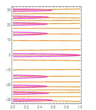

![[Uncaptioned image]](2110.03253v2/anew.png)
![[Uncaptioned image]](2110.03253v2/table666.png)
![[Uncaptioned image]](2110.03253v2/program6.PNG)
![[Uncaptioned image]](2110.03253v2/table17.PNG)
![[Uncaptioned image]](2110.03253v2/code123.png)
![[Uncaptioned image]](2110.03253v2/table777.png)
![[Uncaptioned image]](2110.03253v2/table111.png)
![[Uncaptioned image]](2110.03253v2/table222.png)
![[Uncaptioned image]](2110.03253v2/table333.png)
![[Uncaptioned image]](2110.03253v2/table444.png)
![[Uncaptioned image]](2110.03253v2/table555.png)
![[Uncaptioned image]](2110.03253v2/code_new.PNG)
![[Uncaptioned image]](2110.03253v2/code_NEW.PNG)
![[Uncaptioned image]](2110.03253v2/table1111.png)
![[Uncaptioned image]](2110.03253v2/table2222.png)
![[Uncaptioned image]](2110.03253v2/table5555.png)
![[Uncaptioned image]](2110.03253v2/table6666.png)
![[Uncaptioned image]](2110.03253v2/table66666.png)
![[Uncaptioned image]](2110.03253v2/table00100.png)
![[Uncaptioned image]](2110.03253v2/11table.png)
![[Uncaptioned image]](2110.03253v2/222table.png)
![[Uncaptioned image]](2110.03253v2/33table.png)
![[Uncaptioned image]](2110.03253v2/001100table.png)


![[Uncaptioned image]](2110.03253v2/tab.PNG)
![[Uncaptioned image]](2110.03253v2/tab10.PNG)


![[Uncaptioned image]](2110.03253v2/tab11.PNG)

![[Uncaptioned image]](2110.03253v2/tab12.PNG)
![[Uncaptioned image]](2110.03253v2/tab13.PNG)
![[Uncaptioned image]](2110.03253v2/tab14-1.PNG)
![[Uncaptioned image]](2110.03253v2/tab14-2.PNG)