Unsupervised Selective Labeling for More Effective Semi-Supervised Learning
Abstract
Given an unlabeled dataset and an annotation budget, we study how to selectively label a fixed number of instances so that semi-supervised learning (SSL) on such a partially labeled dataset is most effective. We focus on selecting the right data to label, in addition to usual SSL’s propagating labels from labeled data to the rest unlabeled data. This instance selection task is challenging, as without any labeled data we do not know what the objective of learning should be. Intuitively, no matter what the downstream task is, instances to be labeled must be representative and diverse: The former would facilitate label propagation to unlabeled data, whereas the latter would ensure coverage of the entire dataset. We capture this idea by selecting cluster prototypes, either in a pretrained feature space, or along with feature optimization, both without labels. Our unsupervised selective labeling consistently improves SSL methods over state-of-the-art active learning given labeled data, by in label efficiency. For example, it boosts FixMatch by 10% (14%) in accuracy on CIFAR-10 (ImageNet-1K) with 0.08% (0.2%) labeled data, demonstrating that small computation spent on selecting what data to label brings significant gain especially under a low annotation budget. Our work sets a new standard for practical and efficient SSL.
Keywords:
semi-supervised learning unsupervised selective labeling1 Introduction
Deep learning’s success on natural language understanding [22], visual object recognition [48], and object detection [34] follow a straightforward recipe: better model architectures, more data, and scalable computation [49, 35, 42, 81]. As training datasets get bigger, their full task annotation becomes infeasible [4, 70].
Semi-supervised learning (SSL) deals with learning from both a small amount of labeled data and a large amount of unlabeled data: Labeled data directly supervise model learning, whereas unlabeled data help learn a desirable model that makes consistent [65, 72, 80, 50, 5, 4, 70, 76] and unambiguous [36, 50, 5] predictions.
Recent SSL methods approach fully supervised learning performance with a very small fraction of labeled data. For example, on ImageNet, SSL with 1% labeled data, i.e., only 13 instead of around 1300 labeled images per class, captures 95% (76.6% out of 80.5% in terms of top-1 accuracy) of supervised learning performance with 100% fully labeled data [16].
The lower the annotation level, the more important what the labeled instances are to SSL. While a typical image could represent many similar images, an odd-ball only represents itself, and labeled instances may even cover only part of the data variety, trapping a classifier in partial views with unstable learning and even model collapse.

|
|
|

A common assumption in SSL is that labeled instances are sampled randomly either over all the available data or over individual classes, the latter known as stratified sampling [5, 4, 70, 76]. Each method has its own caveats: Random sampling can fail to cover all semantic classes and lead to poor performance and instability, whereas stratified sampling is utterly unrealistic: If we can sample data by category, we would already have the label of every instance!
Selecting the right data to label for the sake of model optimization is not new. In fact, it is the focus of active learning (AL): Given an initial set of labeled data, the goal is to select an additional subset of data to label (Fig. 1) so that a model trained over such partially labeled data approaches that over the fully labeled data [66, 28, 84]. Unlabeled data can also be exploited for model training by combining AL and SSL, resulting in a series of methods called semi-supervised active learning (SSAL).
However, existing AL/SSAL methods have several shortcomings.
- 1.
They often require randomly sampled labeled data to begin with, which is sample-inefficient in low labeling settings that SSL methods excel at [14].
- 2.
AL/SSAL methods are designed with human annotators in a loop, working in multiple rounds of labeling and training. This could be cumbersome in low-shot scenario and leads to large labeling overhead.
- 3.
AL’s own training pipeline with a human-in-the-loop design makes its integration into existing SSL code implementation hard [71].
- 4.
The requested labels are tightly coupled with the model being trained so that labels need to be collected anew every time a model is trained with AL/SSAL.
We address unsupervised selective labeling for SSL (Fig. 1), in stark contrast with supervised data selection for AL, which is conditioned on an initial labeled set and for the benefit of a certain task. Given only an annotation budget and an unlabeled dataset, among many possible ways to select a fixed number of instances for labeling, which way would lead to the best SSL model performance when it is trained on such partially labeled data?
Our instance selection task is challenging, as without any labeled data we do not know what the objective of learning should be. Intuitively, no matter what the downstream task is, instances to be labeled must be representative and diverse: The former would facilitate label propagation to unlabeled data, whereas the latter would ensure coverage of the entire dataset. We capture this idea by selecting cluster prototypes, either in a pretrained feature space, or along with feature optimization, both without labels.
Our pipeline has three steps: 1) Unsupervised feature learning that maps data into a discriminative feature space. 2) Select instances for labeling for maximum representativeness and diversity, without or with additional optimization. 3) Apply SSL (e.g., [70, 16]) to the labeled data and the rest unlabeled data.
Fig. 2 shows that our method has many benefits over random or stratified sampling for labeled data selection, in terms of accuracy, coverage, balance over classes, and representativeness. As it selects informative instances without initial labels, it can not only integrate readily into existing SSL methods, but also achieve higher label efficiency than SSAL methods. While most AL/SSAL methods only work on small-scale datasets such as CIFAR[47], our method scales up easily to large-scale datasets such as ImageNet[64], taking less than an hour for our data selection on a commodity GPU server.
Our work sets a new standard for practical SSL with these contributions.
- 1.
We systematically analyze the impact of different selective labeling methods on SSL under low-label settings, a previously ignored aspect of SSL.
- 2.
We propose two unsupervised selective labeling methods that capture representativeness and diversity without or along with feature optimization.
- 3.
We benchmark extensively on our data selection with various SSL methods, delivering much higher sample efficiency over sampling in SSL or AL/SSAL.
- 4.
We release our toolbox with AL/SSL implementations and a unified data loader, including benchmarks, selected instance indices, and pretrained models that combine selective labeling with various methods for fair comparisons.
2 Selective Labeling for Semi-supervised Learning
Suppose we are given an unlabeled dataset of instances and an annotation budget of . Our task is to select () instances for labeling, so that a SSL model trained on such a partially labeled dataset, with instances labeled and unlabeled, produces the best classification performance.
Formally, let denote pairs of image and its (unknown) class label . Let denote a size- subset of with known class labels. Our goal is to select for acquiring class labels, in order to maximize the performance of a given SSL model trained on labeled data and unlabeled data .
Our unsupervised selective labeling is challenging, as we do not have any labels to begin with, i.e., we don’t know what would make the SSL model perform the best. Our idea is to select instances that are not only representative of most instances, but also diverse enough to broadly cover the entire dataset, so that we do not lose information prematurely before label acquisition.
Our SSL pipeline with selective labeling consists of three steps: 1) unsupervised feature learning; 2) unsupervised instance selection for annotation; 3) SSL on selected labeled data and remaining unlabeled data .
We propose two selective labeling methods in Step 2, training-free Unsupervised Selective Labeling (USL) and training-based Unsupervised Selective Labeling (USL-T), both aiming at selecting cluster prototypes in a discriminative feature space without label supervision.
2.1 Unsupervised Representation Learning
Our first step is to obtain lower-dimensional and semantically meaningful features with unsupervised contrastive learning [78, 58, 40, 15], which maps onto a -dimensional hypersphere with normalization, denoted as . We use MoCov2 [18] (SimCLR [15] or CLD [75]) to learn representations on ImageNet (CIFAR [47]). See appendix for details.
2.2 Unsupervised Selective Labeling (USL)
We study the relationships between data instances using a weighted graph, where nodes denote data instances in the (normalized) feature space , and edges between nodes are attached with weights of pairwise feature similarity [7, 26, 20, 68], defined as , the inverse of feature distance :
| (1) |
Intuitively, the smaller the feature distance, the better the class information can be transported from labeled nodes to unlabeled nodes. Given a labeling budget of instances, we aim to select instances that are not only similar to others, but also well dispersed to cover the entire dataset.
Representativeness: Select Density Peaks.
A straightforward approach is to select well connected nodes to spread semantic information to nearby nodes. It corresponds to finding a density peak in the feature space. The -nearest neighbor density (-NN) estimation [31, 59] is formulated as:
| (2) |
where is the volume of a unit -dimensional ball, the feature dimension, the Gamma function, instance ’s th nearest neighbor. is very sensitive to noise, as it only takes the th nearest neighbor into account. For robustness, we replace the th neighbor distance with the average distance to all nearest neighbors instead:
| (3) |
We use to measure the representativeness of node . Since only the relative ordering matters in our selection process, the density peak corresponds to the sample with maximum (i.e., maximum ).
Diversity: Pick One in Each Cluster.
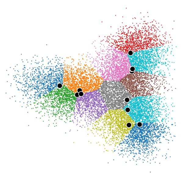
While instances of high feature density values are individually representative, a separate criterion is necessary to avoid repeatedly picking similar instances near the same density peaks (Fig. 3a). To select diverse instances that cover the entire unlabeled dataset, we resort to -Means clustering that partitions instances into ) clusters, with each cluster represented by its centroid [54, 32] and every instance assigned to the cluster of the nearest centroid. Formally, we seek -way node partitioning that minimizes the within-cluster sum of squares[46]:
| (4) | ||||
It is optimized iteratively with EM [55] from random initial centroids. We then pick the most representative instance of each cluster according to Eqn. 3.
 |
 |
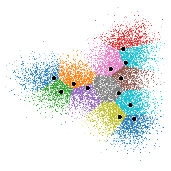 |
| a) local only | b) local global | c) local global reg. |
Regularization: Inter-cluster Information Exchange.
So far we use -Means clustering to find hard clusters, and then choose the representative of each cluster independently. This last step is sub-optimal, as instances of high density values could be located along cluster boundaries and close to instances in adjacent regions (Fig. 3b). We thus apply a regularizer to inform each cluster of other clusters’ choices and iteratively diversify selected instances (Fig. 3c).
Specifically, let denote the set of instances selected at iteration , for clusters , where . For each candidate in cluster , the farther it is away from those in other clusters in , the more diversity it creates. We thus minimize the total inverse distance to others in a regularization loss , with a sensitivity hyperparameter :
| (5) |
This regularizer is updated with an exponential moving average:
| (6) |
where is the momentum. At iteration , we select instance of the maximum regularized utility within each cluster:
| (7) |
where is a hyperparameter that balances diversity and individual representativeness, utility . In practice, calculating distances between every candidate and every selected instance in is no longer feasible for a large dataset, so we only consider nearest neighbors in . at the last iteration is our final selection for labeling.
2.3 Training-Based Unsupervised Selective Labeling (USL-T)
Our USL is a simple yet effective training-free approach to selective labeling. Next we introduce an end-to-end training-based Unsupervised Selective Labeling (USL-T), an alternative that integrates instance selection into representation learning and often leads to more balanced (Fig. 5) and more label-efficient (Table 2) instance selection. The optimized model implicitly captures semantics and provides a strong initialization for downstream tasks (Sec. 4.5).
Global Constraint via Learnable -Means Clustering.
Clustering in a given feature space is not trivial (Fig. 3c). We introduce a better alternative to -Means clustering that jointly learns both the cluster assignment and the feature space for unsupervised instance selection.
Suppose that there are centroids initialized randomly. For instance with feature , we infer one-hot cluster assignment distribution by finding the closest learnable centroid based on feature similarity :
| (8) |
We predict a soft cluster assignment by taking softmax over the similarity between instance and each learnable centroid:
| (9) |
The hard assignment can be regarded as pseudo-labels[50, 70, 74]. By minimizing , the KL divergence between soft and hard assignments, we encourage not only each instance to become more similar to its centroid, but also the learnable centroid to become a better representative of instances in the cluster. With soft predictions, each instance has an effect on all the centroids.
Hardening soft assignments has a downside: Initial mistakes are hard to correct with later training, degrading performance. Our solution is to ignore ambiguous instances with maximal softmax scores below threshold :
| (10) |
where is the threshold hyper-parameter. This loss leads to curriculum learning: As instances are more confidently assigned to a cluster with more training, more instances get involved in shaping both feature and clusters .
Our global loss can be readily related to -Means clustering.
Observation 2.1
For and fixed feature , optimizing is equivalent to optimizing -Means clustering with a regularization term on inter-cluster distances that encourage additional diversity. See Appendix for derivations.
Local Constraint with Neighbor Cluster Alignment.
Our global constraint is the counterpart of -Means clustering in USL. However, since soft assignments usually have low confidence scores for most instances at the beginning, convergence could be very slow and sometimes unattainable. We propose an additional local smoothness constraint by assigning an instance to the same cluster of its neighbors’ in the unsupervisedly learned feature space to prepare confident predictions for the global constraint to take effect.
This simple idea as is could lead to two types of collapses: Predicting one big cluster for all the instances and predicting a soft assignment that is close to a uniform distribution for each instance. We tackle them separately.
1) For one-cluster collapse, we adopt a trick for long-tailed recognition [56] and adjust logits to prevent their values from concentrating on one cluster:
| (11) | ||||
| (12) |
where controls the intensity of adjustment, is an exponential moving average of , and is the softmax function.
2) For even-distribution collapse, we use a sharpening function [5, 4, 2] to encourage the cluster assignment to approach a one-hot probability distribution, where a temperature parameter determines the spikiness.
Both anti-collapse measures can be concisely captured in a single function that modifies and turns logits into a reference distribution:
| (13) |
We now impose our local labeling smoothness constraints with such modified soft assignments between and its randomly selected neighbor :
| (14) |
We restrict to ’s nearest neighbors, selected according to the unsupervisedly learned feature prior to training and fixed for simplicity and efficiency.
We show that our local constraint prevents both collapses.
Observation 2.2
Neither one-cluster nor even-distribution collapse is optimal to our local constraint, i.e., . See Appendix for more details.
Our final loss adds up the global and local terms with loss weight :
| (15) |
Diverse and Representative Instance Selection in USL-T.
Our USL-T is an end-to-end unsupervised feature learning method that directly outputs clusters for selecting diverse instances. For each cluster, we then select the most representative instance, characterized by its highest confidence score, i.e. . Just as USL, USL-T improves model learning efficiency by selecting diverse representative instances for labeling, without any label supervision.
2.4 Distinctions and Connections With SSL/AL/SSAL
| Property | Semi-supervised Learning | Active Learning | Semi-supervised Active Learning | Ours |
| Uses no initial random labels | ✗ | ✗ | ✗ | ✓ |
| Actively queries for labels | ✗ | ✓ | ✓ | ✓ |
| Requires annotation only once | ✓ | ✗ | ✗ | ✓ |
| Leverages unlabeled data | ✓ | ✗ | ✓ | ✓ |
| Allows label reuse across runs | ✓ | ✗ | ✗ | ✓ |
Table 1 compares our USL with related SSL, AL, and SSAL settings.
- 1.
Our USL has the advantage of AL/SSAL that seeks optimal instances to label, yet does not require inefficient initial random samples or multiple rounds of human interventions. USL has high label efficiency for selected instances in low label settings and does not need to trade off annotation budget allocation between initial random sampling and several interim annotation stages.
- 2.
Compared to AL, our USL also leverages unlabeled data. Compared to SSAL, USL is much easier to implement because we keep existing SSL implementation intact, while SSAL requires a human-in-the-loop pipeline. Consequently, unlike AL/SSAL where instance selection is coupled with the model to be trained, our selection is decoupled from the downstream SSL model. The same selection from USL works well even across different downstream SSL methods, enabling label reuse across different SSL experiments.
- 3.
Most notably, our work is the first unsupervised selective labeling method on large-scale recognition datasets that requests annotation only once.
3 Related Work
Semi-supervised Learning
(SSL) integrates information from small-scale labeled data and large-scale unlabeled data. Consistency-based regularization [65, 72, 80] applies a consistency loss by imposing invariance on unlabeled data under augmentations. Pseudo-labeling [50, 5, 4, 76] relies on the model’s high confidence predictions to produce pseudo-labels of unlabeled data and trains them jointly with labeled data. FixMatch [70] integrates strong data augmentation [23] and pseudo-label filtering[53] and explores training on the most representative samples ranked by [10]. However, [10] is a supervised method that requires all labels. Transfer learning method SimCLRv2 [16] is a two-stage SSL method that applies contrastive learning followed by fine-tuning on labeled data. Entropy-minimization [36, 5] assumes that classification boundaries do not pass through the high-density area of marginal distributions and enforces confident predictions on unlabeled data. Instead of competing with existing SSL methods, our USL enables more effective SSL by choosing the right instances to label for SSL, without any prior semantic supervision.
Active Learning
(AL) aims to select a small subset of labeled data to achieve competitive performance over supervised learning on fully labeled data [21, 63, 6]. Traditional AL has three major types [67, 62]: membership query synthesis [1], stream-based selective sampling [24, 3], and pool-based active learning [73, 43, 77, 57]. In Deep AL, Core-Set [66] approaches data selection as a set cover problem. [28] estimates distances from decision boundaries based on sensitivity to adversarial attacks. LLAL [84] predicts target loss of unlabeled data parametrically and queries instances with the largest loss for labels. Semi-supervised Active Learning (SSAL) combines AL with SSL. [71] merges uncertainty-based metrics with MixMatch[5]. [33] merges consistency-based metrics with consistency-based SSL. AL/SSAL often rely on initial labeled data to learn both the model and the instance sampler, requiring multiple (e.g. 10) rounds of sequential annotation and significant modifications of existing annotation pipelines. Recent few-label transfer[52] leverages features from a large source dataset to select instances in a smaller target dataset for annotation. It also requires a seed instance per class to be pre-labeled in the target dataset, whereas we do not need supervision anywhere for our instance selection.
Deep Clustering.
DeepCluster [11] also jointly learns features and cluster assignments with -Means clustering. However, USL-T, with end-to-end backprop to jointly optimize classifiers and cluster assignments, is much more scalable and easy to implement. UIC/DINO [17, 13] incorporate neural networks with categorical outputs through softmax, but both methods focus on learning feature or attention maps for downstream applications instead of acquiring a set of instances that are representative and diverse. Recently, SCAN/NNM/RUC [74, 25, 60] produce image clusters to be evaluated against semantic classes via Hungarian matching. However, such methods are often compared against SSL methods [74], whereas our work is for SSL methods. See appendix for more discussions about self-supervised learning and deep clustering methods.
4 Experiments
We evaluate our USL and USL-T by integrating them into both pseudo-label based SSL methods (FixMatch [70], MixMatch [5], or CoMatch[51]) and transfer-based SSL methods (SimCLRv2 and SimCLRv2-CLD[16, 75]). We also compare against various AL/SSAL methods. Lastly, we show several intriguing properties of USL/USL-T such as generalizability.
| CIFAR-10 | Budget | Acc (%) |
| Active Learning (AL) | ||
| CoreSet[66]† | 7500 | 85.4 |
| VAAL[69]† | 7500 | 86.8 |
| UncertainGCN[9]† | 7500 | 86.8 |
| CoreGCN[9]† | 7500 | 86.5 |
| MCDAL[19] | 7500 | 87.2 |
| Semi-supervised Active Learning (SSAL) | ||
| TOD-Semi[44] | 7500 | 87.8 |
| CoreSetSSL[66]‡ | 250 | 88.8 |
| CBSSAL [33] | 150 | 87.6 |
| MMA[71] | 500 | 91.7 |
| MMA+k-means[71] | 500 | 91.5 |
| REVIVAL[38] | 150 | 88.0 |
| Selective Labeling | ||
| FixMatch + USL (Ours) | 40 | 90.4 |
| FixMatch + USL (Ours) | 100 | 93.2 |
| FixMatch + USL-T (Ours) | 40 | 93.5 |
4.1 CIFAR-10
| CIFAR-10 | S.v2-CLD | FixMatch |
| Random Selection | 60.8 | 82.9 |
| Stratified Selection† | 66.5 | 88.6 |
| UncertainGCN | 63.0 | 77.3 |
| CoreGCN | 62.9 | 72.9 |
| MMA+‡ | 60.2 | 71.3 |
| TOD-Semi | 65.1 | 83.3 |
| USL (Ours) | 76.6 11.5 | 90.4 7.1 |
| USL-T (Ours) | 76.1 11.0 | 93.5 10.2 |
We compare against mainstream SSL methods such as FixMatch[70] and SimCLRv2-CLD[16, 75] on extremely low-label settings to demonstrate our superior label efficiency. The labeling budget is 40 samples in total unless otherwise stated. Note that the self-supervised models used for instance selection are trained on CIFAR-10 from scratch entirely without external data. The SSL part, including backbone and hyperparameters, is untouched. See appendix for details.
Comparison with AL and SSAL.
Table 2 compares ours against various recent AL/SSAL methods in terms of sample efficiency and accuracy. AL methods operate at a much larger labeling budget than ours ( more), because they rely only on labeled samples to learn both features and classification. SSAL methods make use of unlabeled samples and have higher label efficiency. However, we achieve much higher accuracy with fewer labels requested.
To tease apart whether our performance gains come from SSL or selective labeling, we tune recent AL/SSAL methods with their public implementations and run experiments with the same total budget, i.e. 40 samples in a 20 random + 20 selected setting. We then apply AL/SSAL selections to the same SSL for a fair comparison (Table 3).
While AL performs better than random selection in SimCLRv2-CLD, its advantage saturates on FixMatch. Since AL relies on labeled samples to learn the right features, with 20 random samples, it is very difficult to learn meaningful features for selection. Instead, AL could only learn a very coarse selection criterion and hence limited gains.
SSAL methods have greater gains on SimCLRv2-CLD. However, since SSAL still depends on initial random selections which seldom cover all 10 classes, these methods do not have an accurate knowledge of the full dataset in the low-label setting, where many rounds of queries are infeasible. That is, there is a serious trade-off in the low-label regime: Allowing more samples (e.g., 30) in the initial random selection for better coverage means less annotation budget for AL/SSAL selection (e.g., 10). Such a dilemma manifests itself in the imbalanced selection in Fig. 5 and the poor performance on FixMatch.
4.2 CIFAR-100
On CIFAR-100, we keep hyperparameters the same as the ones for CIFAR-10, except that we change the budget level to to have 4 labels per class on average. Although we may benefit more from hyperparameter tuning, we already show consistent gains over other selection methods (Table 6).
| CIFAR-10 | MixMatch | SimCLRv2 | SimCLRv2-CLD | FixMatch | CoMatch |
| Random | 43.4 | 55.9 | 60.8 | 82.9 | 87.4 |
| Stratified | 62.0 | 69.8 | 66.5 | 88.6 | 93.1 |
| USL (Ours) | 61.6 18.2 | 69.1 13.2 | 76.6 15.8 | 90.4 7.5 | 93.4 6.0 |
| USL-T (Ours) | 66.0 22.6 | 71.5 15.6 | 76.1 15.3 | 93.5 10.6 | 93.0 5.6 |
4.3 ImageNet-100 and ImageNet-1k
To demonstrate our effectiveness on large-scale datasets, we benchmark on 100 random classes of ImageNet [74] and the full ImageNet [64].
ImageNet-100.
On SimCLRv2 with a budget of 400 labels in total, we outperform baselines by 6.1% in this extremely low-label setting (Table 6).
| CIFAR-100 | S.v2-CLD Acc | FixMatch Acc |
| Random Selection | 26.5 | 48.7 |
| Stratified Selection† | 30.6 | 51.2 |
| USL (Ours) | 33.0 6.5 | 55.1 6.4 |
| USL-T (Ours) | 36.9 10.4 | 55.7 7.0 |
| ImageNet-100 | SimCLRv2 Acc |
| Random | 62.2 |
| Stratified† | 65.1 |
| USL (Ours) | 67.5 5.3 |
| USL-T (Ours) | 68.3 6.1 |
| SimCLRv2 | FixMatch | |||
| ImageNet-1k | 1% | 0.20% | 1% | 0.20% |
| Random | 49.7 | 33.2 | 58.8 | 34.3 |
| Stratified† | 52.0 | 36.4 | 60.9∗ | 41.1 |
| USL-MoCo (Ours) | 51.5 1.8 | 39.8 6.6 | 61.6 2.8 | 48.6 14.3 |
| USL-CLIP (Ours) | 52.6 2.9 | 40.4 7.2 | 62.2 3.4 | 47.5 13.2 |
ImageNet-1k: Setup.
We experiment on SimCLRv2 and FixMatch with 1% ( labels) and 0.2% ( labels) labeled data. We also design a variant of our method that utilizes features provided by CLIP [61]. CLIP is trained on uncurated internet-crawled data in a wide range of domains. Following [8], we initialize FixMatch parameters with MoCov2. See appendix for more details.
ImageNet-1k: Comparing With AL/SSAL Methods.
As most AL/SSAL methods in Table 2 do not scale to ImageNet, we compare our USL with SSAL methods specifically designed for ImageNet-scale settings [29]. Fig. 4(b) shows our improvement in terms of label efficiency. Table 7 shows that our approach provides up to 14.3% (3.4%) gains in the 0.2% (1%) SSL setting.
ImageNet-1k: USL-CLIP.
Table 7 shows samples selected according to both MoCov2 and CLIP features boost SSL performance. USL-MoCo performs 1.1% better than USL-CLIP in the FixMatch setting. We hypothesize that it is, in part, due to a mismatch between parameter initialization (MoCov2) and the feature space used for the sampling process (CLIP). However, for 1% case, USL-CLIP performs 0.6% better than USL-MoCo, showing a slight advantage of a model trained with sufficient general knowledge and explicit semantics.
4.4 Strong Generalizability
Cross-dataset Generalizability with CLIP.
Since CLIP does not use ImageNet samples in training and the downstream SSL task is not exposed to the CLIP model either, USL-CLIP’s result shows strong cross-dataset generalizability in Table 7. It means that: 1) When a new dataset is collected, we could use a general multi-modal model to skip self-supervised pretraining; 2) Unlike AL where sample selection is strictly coupled with model training, our annotated instances work universally rather than with only the model used to select them.
Cross-domain Generalizability.
Such generalizability also holds across domains. We use a CLD model trained on CIFAR-10 to select 40 labeled instances in medical imaging dataset BloodMNIST [82]. Although our model has not been trained on any medical images, our model with FixMatch performs 10.9% (7.6%) better than random (stratified) sampling. See appendix for more details.
4.5 USL-T for Representation Learning
Our USL-T updates feature backbone weights during selective labeling. The trained weights are not used as a model initializer in the downstream SSL experiments for fair comparisons. However, we discover surprising generalizability that greatly exceeds self-supervised learning models under the SimCLRv2 setting. Specifically, we compare the performance of classifiers that are initialized with various model weights and are optimized on samples selected by different methods. Table 9 shows that, even with these strong baselines, initializing the model with our USL-T weights surpasses baselines by 8.2%.
| CIFAR- | ImageNet- | |
| Hyperparam | 10/100 | 100/1k |
| Adjustment Factor | 5 | 2.5 |
| Temperature | 0.25 | 0.5 |
| Loss Term Weight | 5 | 0.5 |
| Neighborhood Size | 20 | |
| Momentum | 0.5 | |
4.6 Hyperparameters and Run Time
Table 9 shows that our hyperparameters generalize within small-scale and large-scale datasets. Our computational overhead is negligible. On ImageNet, we only introduce about 1 GPU hour for selective labeling, as opposed to 2300 GPU hours for the subsequent FixMatch pipeline. See appendix for more analysis, including formulations and visualizations.
5 Summary
Unlike existing SSL methods that focus on algorithms that better integrate labeled and unlabeled data, our selective-labeling is the first to focus on unsupervised data selection for labeling and enable more effective subsequent SSL. By choosing a diverse representative set of instances for annotation, we show significant gains in annotation efficiency and downstream accuracy, with remarkable selection generalizability within and across domains.
Acknowledgements.
The authors thank Alexei Efros and Trevor Darrell for helpful discussions and feedback on this work in their classes.
6 Appendix
6.1 Relationships Between Global Loss in USL-T and the K-Means Clustering Objective
Intuitively, the global loss in our proposed USL-T performs deep clustering. Furthermore, a connection can be observed between minimizing global loss and performing a generalized form of K-Means clustering, which reduces to K-Means clustering with an additional regularization term when and the feature space is fixed.
Observation 6.1
Assume that and the feature space is fixed, minimizing optimizes the objective of -Means clustering with a regularization term on the inter-cluster distance that encourages additional diversity.
Proof
Recall that we have one-hot assignment and soft assignment defined as:
| (16) |
| (17) |
where are learnable centroids with feature dimension , is a function that quantifies the similarity between two points in a feature space and is a function that maps an input to a feature space, which is implemented by a CNN.
Then our global loss is defined as:
| (18) |
When , the filtering function has no effect. Then we can simplify our global loss and turn the loss into the following form:
| (19) |
Since the feature space is fixed, i.e. does not change across the loss optimization, remains constant, and the goal is to find the optimal centroids that minimizes the loss:
| (20) |
We then get:
| (21) | ||||
| (22) | ||||
| (23) |
Since is a one-hot vector, we can simplify equation 23 further. Define and for some metric ,
| (24) | ||||
| (25) | ||||
| (26) | ||||
| (27) | ||||
| (28) |
If we let be squared L2 distance, the expression can be decomposed into the sum of a square L2 distance with an regularization term:
| (29) |
where
| Main objective | (30) | |||
| Reg | (31) |
Minimizing the regularization term is equivalent to maximizing the sample’s distance to all clusters , . This pushes apart different clusters and contributes to the diversity between clusters:
For , there is only force from the regularization term, which pushes apart a sample and other clusters that it does not belong to.
For , there are two forces: one from the main objective (equation 30) and one from the regularization term (equation 31). The regularization term pushes the sample away from its assigned cluster, i.e. the regularization term maximizes also for , while the main objective minimizes .
We can quantify the net effect for scenario. The gradient of the regularization term w.r.t is , and the gradient from the main objective to is always 1. As is a probability distribution, . Therefore, the net effect is still minimizing , i.e. attracting to its cluster center and to .
Therefore, equation 31 is a regularization term aiming for additional diversity.
Now we consider the objective without the regularization term, and we define the centroids without the regularization term as:
| (32) |
| (34) | ||||
| (35) |
Then the solution to equation 34 is to minimize the individual , i.e. the sum of squared L2 distances between a cluster and the samples that belong to it.
Without loss of generalizability, we analyze ,
| (36) | ||||
| (37) |
The gradient of the objective in equation 37 w.r.t is
| (38) |
since the objective is convex, equation 38 indicates the unique minimum is reached when
| (39) | ||||
| (40) |
This means that is the mean of all sample vectors that belong to cluster . This indicates that equation 32 is equivalent to the objective of -Means clustering, which aims to minimize the square L2 distance between a group of samples that are assigned to a specific cluster and the mean of this group of samples.
Therefore, has same objective with -Means clustering with an extra regularization term on maximizing the inter-cluster sample distances for cluster diversity.
6.2 Non-optimality of Two Types of Collapses
Observation 6.2
Neither one-cluster nor even-distribution collapse is optimal to our local constraint, i.e. for either collapse.
Proof
Let be the logits of and be the moving average of the batch mean of , with as the softmax function and as the momentum:
| (41) | ||||
| (42) |
Recall that we define our anti-collapsing function with two components, as:
| (43) | ||||
| (44) | ||||
| (45) |
where is the adjustment factor and is the temperature.
Then the local loss is formulated as:
| (47) | ||||
| (48) |
where is a randomly picked neighbor from the nearest neighbors of .
According to Jensen’s inequality, KL divergence only achieves optimality, with gradient norm 0, when . To prove a solution is not optimal for , we only need to prove .
For one-cluster collapse, where the neural network assigns all samples to the same cluster with high confidence, both and are very close to a one-hot distribution, with .
Assuming that we have already taken enough iterations for the moving average to catch up in this collapsing situation, that the difference between and is negligible: . We have:
| (49) | ||||
| (50) | ||||
| (51) |
where is a constant and is a vector of 1 when . With , has an even stronger adjustment effect that pushes the target distribution even farther than uniform distribution, which is found to be beneficial in our circumstances with an optimizer that is using momentum for faster convergence.
Note that is a distribution close to one-hot, as above, we have:
| (52) | ||||
| (53) | ||||
| (54) | ||||
| (55) |
where C is the number of clusters.
Therefore, our loss will drive the distribution back to one that is less extreme, i.e. close to uniform distribution, and thus one-cluster collapse is not an optimum for .
Now we consider even distribution collapse, where samples are assigned to a distribution close to uniform distribution, with mean distribution of all samples being uniform, i.e. the mapping function assigns similar logits and thus similar distributions to all clusters with small variations that are drawn from a distribution with zero-mean. Note that exact uniform distribution, where the variation exactly equals to 0, is hardly achieved in the optimization process and thus is not a concern for us.
Consider one such sample with neighbors and predicted logits from the batch. Here we also assume that the exponential moving average catches up, so that we have: . In this case, :
| (56) | ||||
| (57) | ||||
| (58) |
Note that is by design invariant to an additive constant on the :
| (59) | ||||
| (60) | ||||
| (61) | ||||
| (62) |
Then we consider the net effect of and :
| (63) | ||||
| (64) | ||||
| (65) | ||||
| (66) |
The last step comes from the fact that contains some variations and is not a uniform distribution. In this case, will enlarge the dimension of z which has maximum value and make other dimension smaller in the output probability, forcing the softmax distribution to be spikier during training. Therefore, will have a distribution that makes the variation more significant, driving the distribution out of mean cluster collapse.
6.3 Additional Experiment Results
Varying Budgets.
Table 10 and 11 indicate the accuracy with different budget levels on SimCLRv2-CLD and FixMatch, respectively. For SimCLRv2-CLD, our method consistently outperforms not only random selection but also stratified selection for all the low-label settings. Our improvement is prominent especially when the number of selected samples is low. In 40 (250) labels case, we are able to achieve a 15.8% (2.7%) improvement. For FixMatch, we consistently outperform random baselines and even outperform stratified sampling, which makes use of ground truth labels of unlabeled data, in most of the settings.
| Sampling Method | 40 labels | 100 labels | 250 labels |
| Random | 60.8 | 73.7 | 79.4 |
| Stratified | 66.5 | 74.5 | 80.4 |
| USL (Ours) | 76.6 15.8 | 79.0 5.3 | 82.1 2.7 |
| USL-T (Ours) | 76.1 15.3 | - | - |
| Accuracy (%) | |||
| Sample Selection | 40 labels | 100 labels | 250 labels |
| Random | 82.9 | 88.7 | 93.3 |
| Stratified* | 88.6 | 90.2 | 94.9 |
| USL (Ours) | 90.4 7.5 | 93.2 4.5 | 94.0 0.7 |
| USL-T (Ours) | 93.5 10.6 | - | - |
| ImageNet | SimCLRv2 |
| Random | 33.2 |
| Stratified | 36.4 |
| USL-MoCo (Ours) | 39.8 6.6 |
| USL-CLIP (Ours) | 40.4 7.2 |
| USL-T (Ours) | 41.3 8.1 |
USL-T on ImageNet.
We also provide experimental results of USL-T on ImageNet in Table 12. As for the hyperparams for USL-T, we use the same hyperparams as shown in the hyperparam table in the main text. For ImageNet, to create a fair comparison, USL-T model is initialized with weights of MoCov2.
| Selection Method | Accuracy |
| Random | 77.17 6.98 |
| Stratified | 80.46 7.88 |
| USL (Ours) | 88.06 1.41 10.89 |
Cross-domain Generalizability on MedMNIST.
We show USL’s impressive generalizability in the main text through selective labeling with CLIP features in the ImageNet training set. Furthermore, to analyze whether USL’s generalizability holds across domains, we use the exact same CLD model pretrained on CIFAR-10 to select samples in the BloodMNIST dataset of the MedMNISTv2 collection [82], which is a dataset in medical imaging domain. BloodMNIST contains about 18k blood cell images under microscope in 8 classes, which is drastically different from CIFAR-10’s domain, but as shown in Table 13, our model with FixMatch performs better than random sampling and better than stratified sampling, further illustrating the possibility of a general sample selection model across image domains.
6.4 CIFAR-10 Visualizations on Selected Samples
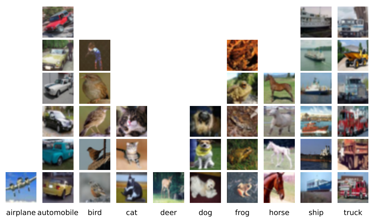
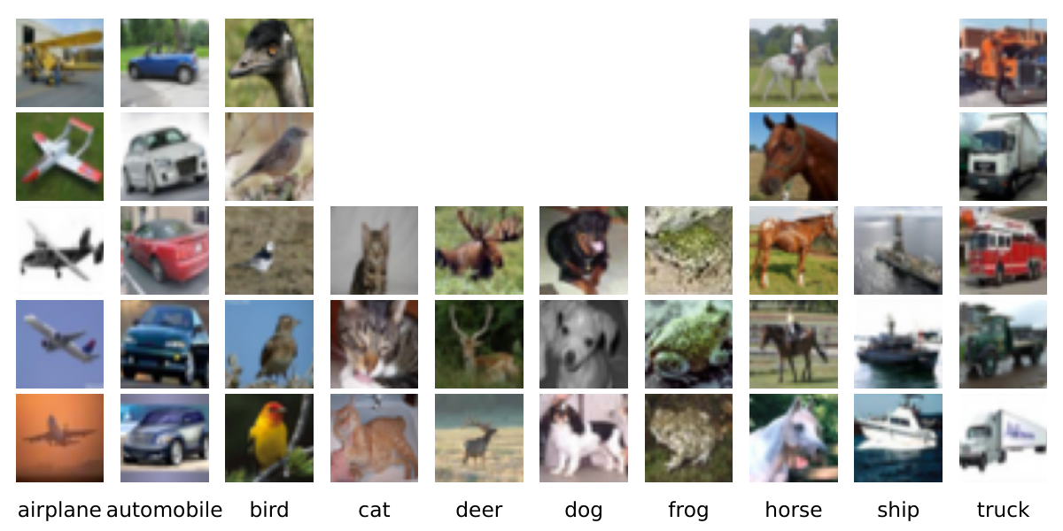
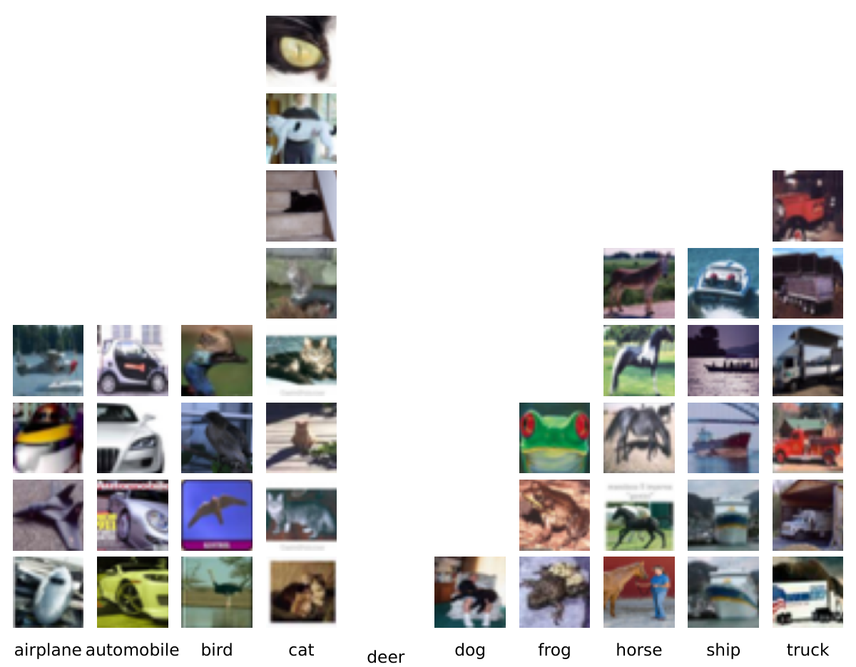
We visualize the top-40 and least-40 of our USL and USL-T selected samples in CIFAR-10, as in Fig. 6. For clarity, we put images into buckets according to their labels. Samples from random selection are highly imbalanced in terms of semantic class distribution and coverage. Our top selected samples from USL and USL-T are representative and diverse. The representativeness could be seen from that the objects are almost always appear without any occlusion or any truncation. In contrast, the 40 samples that we are least likely to select are mainly outliers that could mislead the classifier.

6.5 Pseudo-code for the Regularization Algorithm
We summarize the regularization algorithm in pseudo-code in Alg. 1. In Alg. 1, we first obtain , the selection without regularization, and set the moving average regularizer to 0 for every ; then in each iteration, we update with moving average from a closeness measurement to other previously selected samples, where is the index of current iteration. We re-select samples according to regularized utility at the end of each iteration, with being a balancing factor. In the end, the selection from the last iteration is returned.
6.6 Using Euclidean Distance or Cosine Similarity?
Because the features of all instances are projected to a unit hypersphere with L2 normalization, theoretically, maximizing the cosine similarity between two nodes is equivalent to maximizing the inverse of Euclidean distance between two nodes:
| (67) | ||||
| (68) |
However, empirically, using maximizing the inverse of Euclidean distance as the objective function performs better than maximizing the cosine similarity . The reason is that, when two nodes are very close to each others, is more sensitive to the change of its Euclidean distance, whereas tends to be saturated and insensitive to small changes. Therefore, the function has the desired property of non-saturating and can better focus on the distance difference with closest neighbors.
6.7 General-domain Multi-modal Models: our method on CLIP features
Although our method works well in both small and large scale datasets, there are still two interesting aspects that we would like to explore. 1) In our approach, self-supervised models need to be re-trained for each new dataset, which is time-consuming and could potentially delay the schedule for data annotation in real-world industry. 2) Unsupervised models do not model semantic information explicitly, which may lead to confusion that could potentially be mitigated (e.g. datasets with varying intra-class variance will take regions of different sizes and may be treated differently in an unexpected way).
To address these issues, we put our focus on a large pretrained model that encodes semantic information. Fortunately, the availability of large-scale text-image pairs online makes it possible to train a large-scale model that encodes images in the general domain with semantic information. In this paper, we make use of publicly-available CLIP [61] models, a large-scale collection of models trained on Internet-crawled data with a wide general domain and use CLIP’s image model as feature extractor.
Using models trained on multi-modal datasets resolves the above issues. Even though CLIP is never trained on our target dataset, nor does the categories in its training set match the dataset we are using, using it to select does not degrade our performance of sample selection and labeling pipeline. This indicates that the effectiveness of our label selection does not necessarily depend on whether the same pretrained model is used in the downstream task. In addition, we observe that such substitution even helps with a slightly larger annotation budget, demonstrating the effectiveness of making use of semantic information. Since we only perform inference on the CLIP model, the whole sample selection process could complete in 0.5 hours on a commodity server using one GPU, indicating the possibility of our methods without delaying the schedule of human annotation or modifying the annotation pipeline and enables it to be used by industry on real-world dataset collection.
Note that although CLIP supports zero-shot inference by using text input (e.g. class names) to generate weights for its classifier, it is not always possible to define a class with names or even know all the classes beforehand. Since we only make use of the image part of the CLIP model, we do not make use of prior text information (e.g. class descriptions) that are sometimes available in the real world. We leave better integration of our methods and zero-shot multi-modal models to future work.
6.8 Hyperparameter Analysis
| Small-scale Dataset | Large-scale Dataset | |||||
| Hyperparam | CIFAR-10 | CIFAR-100 | MedMNIST | Hyperparam | ImageNet-100 | ImageNet |
| in NN | 400 | in NN | 20 | |||
| 0.9 | Horizon | 64 | ||||
| , | 0.5, 0.5( 100 samples) / | , | 0.5, 1.5 | |||
| 1.0, 1.0( 100 samples) | ||||||
| Iteration | 10 | |||||
We focus on two hyperparameters in the analysis: , the weight for regularization, and , the number of neighbors we use for NN, in Fig. 7. We use CIFAR-10 with SimCLRv2-CLD in a setting with a budget of 40 samples.
For hyperparam , we evaluated label selections with different values used in regularization. In the experiments, we select , ranging from 0 to 6 in a 0.5 increment, where 0 indicates no regularization and larger indicates a stronger regularization. We then evaluate the mean accuracy from 6 runs (using 2 runs per seed and 3 seeds per setting), the percent of samples that are different when compared to without regularization (i.e., ), and mean density normalized w.r.t. without regularization. We observe that as gets larger, we select more different samples compared to without regularization, which indicates stronger adjustment. This comes with higher accuracy as we have more uniformity. As a trade-off, we could not sample from area which has as high density as before because selecting samples from that area leads to selections that are close to each other, leading to a high penalty. Here, uniformity and representativeness show a trade-off and the optimal choice is to balance each other at around 0.5. When is much greater than 0.5, outlier samples that are as far away as possible from other selections are chosen without considering whether the selected samples are representative, which leads to much lower accuracy.
For hyperparam , we find that using a larger contributes to a better representation estimation by considering more neighbors. Thanks to our formulation that considers not only the sample for density estimation but the distance with all the nearest neighbors, we found that our algorithm’s choice for is very generalizable: we found the optimal for CIFAR-10 to be 400, and found that also performs very well on CIFAR-100 and MedMNIST without any tuning, which indicates our hyperparam’s insensitivity in the number of classes, number of samples per class, and the dataset domain. Similarly, for larger scale datasets with higher image resolution and lower sample noise, we find that simply set leads to good performances on both 100 classes ImageNet and the full ImageNet with 1000 classes.
6.9 Additional Discussions on Related Work
Related Work About Self-supervised Learning.
Self-supervised Learning learns representations transferable to downstream tasks without annotations [78, 37]. Contrastive learning [78, 40, 15, 75] learns representations that map similar samples or different augmentations of the same instance close and dissimilar instances apart. Similarity-based methods [37] learn representations without negative pairs by predicting the embedding of a target network with an online network. Feature learning with grouping [83, 79, 11, 86, 12, 75] respects the natural grouping of data by exploiting clusters in the latent representation. We study unlabeled data in a unsupervisedly learned feature space, due to its high quality and low feature dimensions.
We make use of the high-quality representations and dimensionality-reduction property in self-supervised learning to facilitate sample selection.
Using the representation learned with unsupervised learning as the feature space of selecting labels has two main advantages: 1) Without leveraging any labeled data, self-supervised learning could generate high-quality representations for many downstream tasks. 2) It relieves us from dealing with high-dimensional feature, due to relatively low dimension of output feature.
Related Work About Our Deep Counterpart of -Means Clustering in USL-T.
In USL-T, we proposed a deep counterpart of -Means clustering method that optimizes a unified global objective, which has an effect similar to performing -Means clustering but trains the feature space and cluster assignment jointly. We would like to offer a comparison to main related work of our proposed method that also involves -Means clustering variants or deep clustering designs to jointly learn features and cluster assignments.
Deep -Means [30] proposed a differentiable metric on auto-encoder features to perform clustering. However, [30] only scales to small datasets such as MNIST, while our formulation scales to datasets with around a million images. In addition, while [30] requires a reconstruction term in the loss function to support clustering throughout training, our clustering loss, i.e. global loss, requires only one term that matches the soft and hard distribution. Note that although we also employ a local loss to kick-start the training process due to our confidence-based filtering function, the local loss could be turned off early in the training process without negative impacts on the clustering quality.
DeepCluster [11] also jointly learns features and cluster assignments with -Means clustering. However, our work and [11] have different contributions: while our work adapts -Means clustering to a unified loss formulation, [11] simply uses the traditional -Means as a part of their algorithm to provide supervision for feature learning. In other words, while we directly back-propagation from our adapted -Means algorithm as a global loss term, [11] uses traditional -Means that does not supply gradients and employs another branch for back-propagation and learning purpose. In addition, [11] applies -Means on features of all data, which means all feature needs to be stored prior to clustering, whereas we apply our loss formulation on the current minibatch, which adheres to popular deep learning methods that do not require storing all features from the dataset. USL-T, with end-to-end backprop to jointly solve for cluster assignments and model optimization, is much more scalable and easy to implement.
Recent works [17, 13] on implementing clustering in a deep-learning framework incorporate neural networks that output a categorical distribution through a softmax operator at the end of the network. In addition, DINO [13] also considers the potential collapses and proposes a carefully-designed loss function as mitigation. However, both methods mainly intend to learn a feature space/attention map used for downstream applications instead of acquiring a set of samples that are representative and diverse. Since the feature/attention maps are the goal of designing these methods, the 60k clusters produced by DINO are extremely sparse and highly imbalanced. For ImageNet-1K, 90% clusters from a fully-trained DINO model are empty (vs 0 in USL-T). Therefore, the user has little control over the number of selections in DINO. Empirically, we observe that SSL models optimized on them perform much worse. Furthermore, in our unsupervised selective labeling setting, these methods require full retraining when the downstream budget changes. In contrast, USL-T, which leverages self-supervised pretraining, could complete a selection with new budget constraint with substantially less compute.
Also recently, SCAN/NNM/RUC [74, 25, 60] propose image clustering methods that intend to be evaluated with hungarian matching from image clusters to semantic classes. However, such methods are compared against semi-supervised learning methods [74] instead of being proposed to be combined with semi-supervised learning methods. First of all, these methods make use of all labels on validation split to perform hungarian matching, which implicitly makes use of all the label information. In contrast, our USL/USL-T pipeline follows the standard assumption of semi-supervised learning that no labels, except the ones in the labeled dataset, are leveraged by the method to get the final classification. Furthermore, these methods generally do not generalize well to large datasets such as ImageNet[64], with [25, 60] working on smaller datasets and [74] severely underperforms on ImageNet when a very limited amount (as low as 0.2%) of data labels are available.
6.10 Overview on Unsupervised Representation Learning
In self-supervised learning stage, we aim to learn a mapping function such that in the feature space, the positive instance is attracted to instance , meanwhile, the negative instance (with ) is repelled, and we model by a convolutional neural network, mapping onto a -dimensional hypersphere with normalization. To make a fair comparison with previous arts [8], we use MoCo v2 [18] to learn representations on ImageNet with the instance-centric contrastive loss:
| (69) | ||||
where is a regulating temperature. Minimizing it can be viewed as maximizing the mutual information (MI) lower bound between the features of the same instance [39, 58]. For experiments on ImageNet, the MoCo model pre-trained for 800 epochs is used for initializing the SSL model, as in [8].
The feature spaces of CIFAR-10 data we work on are extracted with CLD [75]. The instance-group contrastive loss is added in symmetrical terms over views and :
| (70) | ||||
Cross-level discrimination of Eqn. 70 (second term) can be understood as minimizing the cross entropy between hard clustering assignment based on and soft assignment predicted from in a different view, where () is instance (group) branch, and denotes the cluster centroid of instance with a cluster id [75]. Empirically, we found that CLD has great feature quality on CIFAR-10 and better respects the underlying semantic structure of data. To be consistent with original FixMatch settings, our semi-supervised learner on CIFAR-10 is trained from scratch, without using pretrained weights.
6.11 Discussions About Run Time
CLD only takes about 4 hours to train on CIFAR-10 on a single GPU and sample selection with USL takes less than 10 minutes on CLD with one GPU. This takes significantly less GPU-time than FixMatch (120 GPU hours with 4 GPUs), which is, in turn, much less than the time for labelling the whole dataset of 50000 samples. On ImageNet, MoCo takes about 12 days with 8 GPUs to achieve 800 epochs [40], our algorithm takes about an hour on one GPU to select samples for both 1% and 0.2% labels, and in the end, FixMatch takes another 20 hours on 4 GPUs to train. Although it sounds like we are using a lot of compute time just to train a self-supervised learning model for selecting what samples to annotate, the fact is that FixMatch requires a self-supervised pretrained checkpoint to work well when the number of labeled samples is low, as shown in [8], even without our selection methods. The only compute overhead introduced is the sample selection process, which is negligible when compared to the other two stages. In addition, shown in our experiments, CLIP, as a model trained on a general and diverse image-text dataset, could also be used to select samples with comparable and sometimes even better samples to label. This indicates that the self-supervised training stage is not required in our method for sample selection when a model that sufficiently covers the current domain is available.
6.12 Experiment Setup and Implementation Details
CIFAR-10/100.
For FixMatch experiments, to maintain consistency with the original FixMatch [70], we evaluate FixMatch trained on CIFAR-10 with steps in total. To illustrate the ability of our algorithm to select informative samples, we evaluate both approaches on an extremely low-label setting from 40 samples to 250 samples in total (4 shots to 25 shots per class on average). Since the original FixMatch is evaluated with stratified sampling on CIFAR-10, we also retrain FixMatch with random sampling with the same number of samples in total as a fair comparison. Unless otherwise stated, we train FixMatch with a learning rate of 0.03, and weight decay on 4 Nvidia RTX 2080 Ti GPUs with batch size 64 for labeled samples and with steps in total. All experiments are conducted with the same training and evaluation recipe for fair comparisons.
For SimCLRv2-CLD, we also evaluate our algorithm on two-stage SSL method SimCLRv2-CLD based on transfer learning [16] by fine-tuning the linear layer of a ResNet-18 pretrained with self-supervised learning algorithm CLD [75]. Specifically, we fine-tune the linear layer on a ResNet-18 trained with CLD [75]. Since it is easy for the network to overfit the few-shot labeled samples, we freeze the backbone and fine-tune only the linear layer. We use SGD with learning rate , momentum , and weight decay for 5 epochs because longer training time will lead to over-fitting.
For MixMatch, we train for 1024 epochs with 1024 steps per epoch, following the original recipe. For each of labeled and unlabeled dataset, we use a batch size 64. We use a learning rate with Adam optimizer. The results are evaluated with an weighted EMA module that has decay rate and are averaged over 20 last epochs in the test set. For CoMatch, we train for 512 epochs with official code and the default recipe.
ImageNet-100/1k.
We evaluate our method on ImageNet [64] with approximately 1 million images and 1000 classes and ImageNet100 [74] with 100 classes from ImageNet.
We use different sets of hyperparameters in large-scale datasets, as described in Sec. 6.8. For USL, we set a finite horizon in the large datasets to make evaluation feasible. Instead of using a momentum in regularization, we run one iteration without momentum for faster selection for both USL-MoCo and USL-CLIP. For USL-T, we freeze the backbone due to computational limitations in large-scale datasets. To maintain consistency with contrastive learning, we use -normed linear layer as the last layer. We also initialize the last layer with features from random samples to greatly speed up convergence. As we find that providing only one label of the sample with top confidence in each cluster does not effectively convey the grouping information in low-shot SSL, we instead query the sample with top density in each cluster and annotate the 20 samples with max density using the label of the requested sample as the pseudo-label. We reduce the iterations in downstream for fair comparison. Similar to [11], we re-initialize centroids of tail or empty clusters to the perturbed centroid of the head cluster. Since this creates centroid competitions that reduce confidence value of the head cluster, we do not make use of confidence value and calculate global loss on all samples by default.
For SimCLRv2 experiments, we fine-tune the released SimCLRv2 checkpoint on baseline selections and our selections. Due to differences in codebases, our reproduced accuracy differs from the one reported on SimCLRv2 paper pretrained and fine-tuned on Cloud TPUs. Therefore, we report our reproduced baseline which is fine-tuned on stratified selection for fair comparison on the effectiveness on sample selection with our method with SimCLRv2. Similar to other ImageNet experiments, we use 1% and 0.2% labeled data. The labeled data selection is the same for SimCLRv2 as for our experiments in FixMatch. To keep the recipe as close to the original implementation as possible, we use ResNet-50[41] with LARS [85] optimizer with learning rate 0.16 and use globally synced batch normalization [45]. While [16] employs a batch size of 1024, we found that under the same number of training epochs, setting batch size to 512 leads to better optimization outcomes on ImageNet-1k in our codebase. This is potentially due to more iterations with the same number of training epochs. Therefore, we set batch sizes to 512 on ImageNet-1k. In addition, to reduce the memory footprint, we use mixed precision training, which has no significant impacts in training accuracy in our observation. We use 60 epochs for 1% task, following [16]. We use 240 epochs for 0.2% task without learning rate decay for all selection methods, since we find this gives better results.
For FixMatch experiments, we use either a MoCo-pretrained model with Exponential Moving Average Normalization (EMAN) [8] or a CLIP ViT/16 model [27] to select samples to annotate. For ImageNet 1%, we run -Means clustering with 12900 clusters, which is slightly more than 12820 samples we are selecting, because we observe that there will sometimes be empty clusters. To maintain consistency with prior works, we use the same setting as in [8] besides the selection of input labeled data, unless otherwise stated. Specifically we use a learning rate of 0.03 with weight decay and train a ResNet-50 for 50 epochs with a MoCo [40] model as pretrained model. We perform learning rate warmup for 5 epochs and decay the learning rate by 0.1 at 30 and 40 epochs. Note that we load MoCo model as the pretrained model for FixMatch for USL-CLIP for fair comparison so that the only difference between MoCo and CLIP setting is the sample selection.
6.13 Details About the Toolbox
Currently, different SSL/AL/SSAL implementations use different formats to represent what samples to label, making selective labeling methods hard to benchmark. Therefore, to standardize the benchmark, we intend to release a toolbox that includes implementations of following methods:
- •
Our selective labeling methods: USL and USL-T
- •
- •
Several AL/SSAL methods that we use as baselines
USL, USL-T, SSL methods, and the AL/SSAL baselines in the toolbox are implemented with unified data loaders that comes with standard and simple file formats to indicate what samples are requested to be labeled and what samples are unlabeled. We provide out-of-the-box data loaders that use this unified file representation for datasets used in our experiments. In addition, the training recipe will be provided for the methods mentioned above to facilitate future research and fair comparisons.
References
- [1] Angluin, D.: Queries and concept learning. Machine learning 2(4), 319–342 (1988)
- [2] Assran, M., Caron, M., Misra, I., Bojanowski, P., Joulin, A., Ballas, N., Rabbat, M.: Semi-supervised learning of visual features by non-parametrically predicting view assignments with support samples. In: Proceedings of the IEEE/CVF International Conference on Computer Vision. pp. 8443–8452 (2021)
- [3] Atlas, L.E., Cohn, D.A., Ladner, R.E.: Training connectionist networks with queries and selective sampling. In: Advances in neural information processing systems. pp. 566–573. Citeseer (1990)
- [4] Berthelot, D., Carlini, N., Cubuk, E.D., Kurakin, A., Sohn, K., Zhang, H., Raffel, C.: Remixmatch: Semi-supervised learning with distribution alignment and augmentation anchoring. arXiv preprint arXiv:1911.09785 (2019)
- [5] Berthelot, D., Carlini, N., Goodfellow, I., Papernot, N., Oliver, A., Raffel, C.: Mixmatch: A holistic approach to semi-supervised learning. arXiv preprint arXiv:1905.02249 (2019)
- [6] Bilgic, M., Getoor, L.: Link-based active learning. In: NIPS Workshop on Analyzing Networks and Learning with Graphs. vol. 4 (2009)
- [7] Bondy, J.A., Murty, U.S.R., et al.: Graph theory with applications, vol. 290. Macmillan London (1976)
- [8] Cai, Z., Ravichandran, A., Maji, S., Fowlkes, C., Tu, Z., Soatto, S.: Exponential moving average normalization for self-supervised and semi-supervised learning. In: Proceedings of the IEEE/CVF Conference on Computer Vision and Pattern Recognition. pp. 194–203 (2021)
- [9] Caramalau, R., Bhattarai, B., Kim, T.K.: Sequential graph convolutional network for active learning. In: Proceedings of the IEEE/CVF Conference on Computer Vision and Pattern Recognition. pp. 9583–9592 (2021)
- [10] Carlini, N., Erlingsson, U., Papernot, N.: Distribution density, tails, and outliers in machine learning: Metrics and applications. arXiv preprint arXiv:1910.13427 (2019)
- [11] Caron, M., Bojanowski, P., Joulin, A., Douze, M.: Deep clustering for unsupervised learning of visual features. In: ECCV (2018)
- [12] Caron, M., Misra, I., Mairal, J., Goyal, P., Bojanowski, P., Joulin, A.: Unsupervised learning of visual features by contrasting cluster assignments. Advances in Neural Information Processing Systems 33 (2020)
- [13] Caron, M., Touvron, H., Misra, I., Jégou, H., Mairal, J., Bojanowski, P., Joulin, A.: Emerging properties in self-supervised vision transformers. In: Proceedings of the IEEE/CVF International Conference on Computer Vision. pp. 9650–9660 (2021)
- [14] Chan, Y.C., Li, M., Oymak, S.: On the marginal benefit of active learning: Does self-supervision eat its cake? In: ICASSP 2021-2021 IEEE International Conference on Acoustics, Speech and Signal Processing (ICASSP). pp. 3455–3459. IEEE (2021)
- [15] Chen, T., Kornblith, S., Norouzi, M., Hinton, G.: A simple framework for contrastive learning of visual representations. In: International conference on machine learning. pp. 1597–1607. PMLR (2020)
- [16] Chen, T., Kornblith, S., Swersky, K., Norouzi, M., Hinton, G.: Big self-supervised models are strong semi-supervised learners. arXiv preprint arXiv:2006.10029 (2020)
- [17] Chen, W., Pu, S., Xie, D., Yang, S., Guo, Y., Lin, L.: Unsupervised image classification for deep representation learning. In: European Conference on Computer Vision. pp. 430–446. Springer (2020)
- [18] Chen, X., Fan, H., Girshick, R., He, K.: Improved baselines with momentum contrastive learning. arXiv preprint arXiv:2003.04297 (2020)
- [19] Cho, J.W., Kim, D.J., Jung, Y., Kweon, I.S.: Mcdal: Maximum classifier discrepancy for active learning. arXiv preprint arXiv:2107.11049 (2021)
- [20] Chung, F.R., Graham, F.C.: Spectral graph theory. No. 92, American Mathematical Soc. (1997)
- [21] Cohn, D., Atlas, L., Ladner, R.: Improving generalization with active learning. Machine learning 15(2), 201–221 (1994)
- [22] Collobert, R., Weston, J., Bottou, L., Karlen, M., Kavukcuoglu, K., Kuksa, P.: Natural language processing (almost) from scratch. Journal of machine learning research 12(ARTICLE), 2493–2537 (2011)
- [23] Cubuk, E.D., Zoph, B., Shlens, J., Le, Q.V.: Randaugment: Practical automated data augmentation with a reduced search space. In: Proceedings of the IEEE/CVF Conference on Computer Vision and Pattern Recognition Workshops. pp. 702–703 (2020)
- [24] Dagan, I., Engelson, S.P.: Committee-based sampling for training probabilistic classifiers. In: Machine Learning Proceedings 1995, pp. 150–157. Elsevier (1995)
- [25] Dang, Z., Deng, C., Yang, X., Wei, K., Huang, H.: Nearest neighbor matching for deep clustering. In: Proceedings of the IEEE/CVF Conference on Computer Vision and Pattern Recognition. pp. 13693–13702 (2021)
- [26] Deo, N.: Graph theory with applications to engineering and computer science. Networks 5(3), 299–300 (1975)
- [27] Dosovitskiy, A., Beyer, L., Kolesnikov, A., Weissenborn, D., Zhai, X., Unterthiner, T., Dehghani, M., Minderer, M., Heigold, G., Gelly, S., et al.: An image is worth 16x16 words: Transformers for image recognition at scale. arXiv preprint arXiv:2010.11929 (2020)
- [28] Ducoffe, M., Precioso, F.: Adversarial active learning for deep networks: a margin based approach. arXiv preprint arXiv:1802.09841 (2018)
- [29] Emam, Z.A.S., Chu, H.M., Chiang, P.Y., Czaja, W., Leapman, R., Goldblum, M., Goldstein, T.: Active learning at the imagenet scale. arXiv preprint arXiv:2111.12880 (2021)
- [30] Fard, M.M., Thonet, T., Gaussier, E.: Deep k-means: Jointly clustering with k-means and learning representations. Pattern Recognition Letters 138, 185–192 (2020)
- [31] Fix, E., Hodges, J.L.: Discriminatory analysis. nonparametric discrimination: Consistency properties. International Statistical Review/Revue Internationale de Statistique 57(3), 238–247 (1989)
- [32] Forgy, E.W.: Cluster analysis of multivariate data: efficiency versus interpretability of classifications. biometrics 21, 768–769 (1965)
- [33] Gao, M., Zhang, Z., Yu, G., Arık, S.Ö., Davis, L.S., Pfister, T.: Consistency-based semi-supervised active learning: Towards minimizing labeling cost. In: European Conference on Computer Vision. pp. 510–526. Springer (2020)
- [34] Girshick, R., Donahue, J., Darrell, T., Malik, J.: Rich feature hierarchies for accurate object detection and semantic segmentation. In: Proceedings of the IEEE conference on computer vision and pattern recognition. pp. 580–587 (2014)
- [35] Goodfellow, I., Bengio, Y., Courville, A.: Deep learning. MIT press (2016)
- [36] Grandvalet, Y., Bengio, Y., et al.: Semi-supervised learning by entropy minimization. CAP 367, 281–296 (2005)
- [37] Grill, J.B., Strub, F., Altché, F., Tallec, C., Richemond, P.H., Buchatskaya, E., Doersch, C., Pires, B.A., Guo, Z.D., Azar, M.G., et al.: Bootstrap your own latent: A new approach to self-supervised learning. arXiv preprint arXiv:2006.07733 (2020)
- [38] Guo, J., Shi, H., Kang, Y., Kuang, K., Tang, S., Jiang, Z., Sun, C., Wu, F., Zhuang, Y.: Semi-supervised active learning for semi-supervised models: Exploit adversarial examples with graph-based virtual labels. In: Proceedings of the IEEE/CVF International Conference on Computer Vision. pp. 2896–2905 (2021)
- [39] Hadsell, R., Chopra, S., LeCun, Y.: Dimensionality reduction by learning an invariant mapping. In: CVPR (2006)
- [40] He, K., Fan, H., Wu, Y., Xie, S., Girshick, R.: Momentum contrast for unsupervised visual representation learning. In: Proceedings of the IEEE/CVF Conference on Computer Vision and Pattern Recognition. pp. 9729–9738 (2020)
- [41] He, K., Zhang, X., Ren, S., Sun, J.: Deep residual learning for image recognition. In: Proceedings of the IEEE conference on computer vision and pattern recognition. pp. 770–778 (2016)
- [42] Hestness, J., Narang, S., Ardalani, N., Diamos, G., Jun, H., Kianinejad, H., Patwary, M., Ali, M., Yang, Y., Zhou, Y.: Deep learning scaling is predictable, empirically. arXiv preprint arXiv:1712.00409 (2017)
- [43] Huang, S.J., Jin, R., Zhou, Z.H.: Active learning by querying informative and representative examples. Advances in neural information processing systems 23, 892–900 (2010)
- [44] Huang, S., Wang, T., Xiong, H., Huan, J., Dou, D.: Semi-supervised active learning with temporal output discrepancy. In: Proceedings of the IEEE/CVF International Conference on Computer Vision. pp. 3447–3456 (2021)
- [45] Ioffe, S., Szegedy, C.: Batch normalization: Accelerating deep network training by reducing internal covariate shift. In: International conference on machine learning. pp. 448–456. PMLR (2015)
- [46] Kriegel, H.P., Schubert, E., Zimek, A.: The (black) art of runtime evaluation: Are we comparing algorithms or implementations? Knowledge and Information Systems 52(2), 341–378 (2017)
- [47] Krizhevsky, A., Hinton, G., et al.: Learning multiple layers of features from tiny images (2009)
- [48] Krizhevsky, A., Sutskever, I., Hinton, G.E.: Imagenet classification with deep convolutional neural networks. Advances in neural information processing systems 25, 1097–1105 (2012)
- [49] LeCun, Y., Bengio, Y., Hinton, G.: Deep learning. nature 521(7553), 436–444 (2015)
- [50] Lee, D.H., et al.: Pseudo-label: The simple and efficient semi-supervised learning method for deep neural networks. In: Workshop on challenges in representation learning, ICML. vol. 3 (2013)
- [51] Li, J., Xiong, C., Hoi, S.C.: Comatch: Semi-supervised learning with contrastive graph regularization. In: Proceedings of the IEEE/CVF International Conference on Computer Vision. pp. 9475–9484 (2021)
- [52] Li, S., Chen, D., Chen, Y., Yuan, L., Zhang, L., Chu, Q., Liu, B., Yu, N.: Improve unsupervised pretraining for few-label transfer. In: Proceedings of the IEEE/CVF International Conference on Computer Vision. pp. 10201–10210 (2021)
- [53] Liu, B., Wu, Z., Hu, H., Lin, S.: Deep metric transfer for label propagation with limited annotated data. In: Proceedings of the IEEE/CVF International Conference on Computer Vision Workshops. pp. 0–0 (2019)
- [54] Lloyd, S.: Least squares quantization in pcm. IEEE transactions on information theory 28(2), 129–137 (1982)
- [55] McLachlan, G.J., Krishnan, T.: The EM algorithm and extensions, vol. 382. John Wiley & Sons (2007)
- [56] Menon, A.K., Jayasumana, S., Rawat, A.S., Jain, H., Veit, A., Kumar, S.: Long-tail learning via logit adjustment. arXiv preprint arXiv:2007.07314 (2020)
- [57] Miao, Z., Liu, Z., Gaynor, K.M., Palmer, M.S., Yu, S.X., Getz, W.M.: Iterative human and automated identification of wildlife images. Nature Machine Intelligence 3(10), 885–895 (2021)
- [58] Oord, A.v.d., Li, Y., Vinyals, O.: Representation learning with contrastive predictive coding. arXiv preprint arXiv:1807.03748 (2018)
- [59] Orava, J.: K-nearest neighbour kernel density estimation, the choice of optimal k. Tatra Mountains Mathematical Publications 50(1), 39–50 (2011)
- [60] Park, S., Han, S., Kim, S., Kim, D., Park, S., Hong, S., Cha, M.: Improving unsupervised image clustering with robust learning. In: Proceedings of the IEEE/CVF Conference on Computer Vision and Pattern Recognition. pp. 12278–12287 (2021)
- [61] Radford, A., Kim, J.W., Hallacy, C., Ramesh, A., Goh, G., Agarwal, S., Sastry, G., Askell, A., Mishkin, P., Clark, J., et al.: Learning transferable visual models from natural language supervision. arXiv preprint arXiv:2103.00020 (2021)
- [62] Ren, P., Xiao, Y., Chang, X., Huang, P.Y., Li, Z., Chen, X., Wang, X.: A survey of deep active learning. arXiv preprint arXiv:2009.00236 (2020)
- [63] Roy, N., Mccallum, A.: Toward optimal active learning through sampling estimation of error reduction. Proceedings of the 18th International Conference on Machine Learning (08 2001)
- [64] Russakovsky, O., Deng, J., Su, H., Krause, J., Satheesh, S., Ma, S., Huang, Z., Karpathy, A., Khosla, A., Bernstein, M., Berg, A.C., Fei-Fei, L.: ImageNet Large Scale Visual Recognition Challenge. International Journal of Computer Vision (IJCV) 115(3), 211–252 (2015). https://doi.org/10.1007/s11263-015-0816-y
- [65] Sajjadi, M., Javanmardi, M., Tasdizen, T.: Regularization with stochastic transformations and perturbations for deep semi-supervised learning. arXiv preprint arXiv:1606.04586 (2016)
- [66] Sener, O., Savarese, S.: Active learning for convolutional neural networks: A core-set approach. arXiv preprint arXiv:1708.00489 (2017)
- [67] Settles, B.: Active learning literature survey (2009)
- [68] Shi, J., Malik, J.: Normalized cuts and image segmentation. IEEE Transactions on pattern analysis and machine intelligence 22(8), 888–905 (2000)
- [69] Sinha, S., Ebrahimi, S., Darrell, T.: Variational adversarial active learning. In: Proceedings of the IEEE/CVF International Conference on Computer Vision. pp. 5972–5981 (2019)
- [70] Sohn, K., Berthelot, D., Carlini, N., Zhang, Z., Zhang, H., Raffel, C.A., Cubuk, E.D., Kurakin, A., Li, C.L.: Fixmatch: Simplifying semi-supervised learning with consistency and confidence. Advances in Neural Information Processing Systems 33 (2020)
- [71] Song, S., Berthelot, D., Rostamizadeh, A.: Combining mixmatch and active learning for better accuracy with fewer labels. arXiv preprint arXiv:1912.00594 (2019)
- [72] Tarvainen, A., Valpola, H.: Mean teachers are better role models: Weight-averaged consistency targets improve semi-supervised deep learning results. In: Proceedings of the 31st International Conference on Neural Information Processing Systems. pp. 1195–1204 (2017)
- [73] Tong, S., Koller, D.: Support vector machine active learning with applications to text classification. Journal of machine learning research 2(Nov), 45–66 (2001)
- [74] Van Gansbeke, W., Vandenhende, S., Georgoulis, S., Proesmans, M., Van Gool, L.: Scan: Learning to classify images without labels. In: European Conference on Computer Vision. pp. 268–285. Springer (2020)
- [75] Wang, X., Liu, Z., Yu, S.X.: Unsupervised feature learning by cross-level instance-group discrimination. In: Proceedings of the IEEE/CVF Conference on Computer Vision and Pattern Recognition. pp. 12586–12595 (2021)
- [76] Wang, X., Wu, Z., Lian, L., Yu, S.X.: Debiased learning from naturally imbalanced pseudo-labels. In: Proceedings of the IEEE/CVF Conference on Computer Vision and Pattern Recognition. pp. 14647–14657 (2022)
- [77] Wei, K., Iyer, R., Bilmes, J.: Submodularity in data subset selection and active learning. In: International Conference on Machine Learning. pp. 1954–1963. PMLR (2015)
- [78] Wu, Z., Xiong, Y., Yu, S.X., Lin, D.: Unsupervised feature learning via non-parametric instance discrimination. In: Proceedings of the IEEE Conference on Computer Vision and Pattern Recognition. pp. 3733–3742 (2018)
- [79] Xie, J., Girshick, R., Farhadi, A.: Unsupervised deep embedding for clustering analysis. In: ICML (2016)
- [80] Xie, Q., Dai, Z., Hovy, E., Luong, T., Le, Q.: Unsupervised data augmentation for consistency training. Advances in Neural Information Processing Systems 33 (2020)
- [81] Xie, Q., Luong, M.T., Hovy, E., Le, Q.V.: Self-training with noisy student improves imagenet classification. In: Proceedings of the IEEE/CVF Conference on Computer Vision and Pattern Recognition. pp. 10687–10698 (2020)
- [82] Yang, J., Shi, R., Wei, D., Liu, Z., Zhao, L., Ke, B., Pfister, H., Ni, B.: Medmnist v2: A large-scale lightweight benchmark for 2d and 3d biomedical image classification. arXiv preprint arXiv:2110.14795 (2021)
- [83] Yang, Y., Xu, D., Nie, F., Yan, S., Zhuang, Y.: Image clustering using local discriminant models and global integration. TIP (2010)
- [84] Yoo, D., Kweon, I.S.: Learning loss for active learning. In: Proceedings of the IEEE/CVF Conference on Computer Vision and Pattern Recognition. pp. 93–102 (2019)
- [85] You, Y., Gitman, I., Ginsburg, B.: Large batch training of convolutional networks. arXiv preprint arXiv:1708.03888 (2017)
- [86] Zhuang, C., Zhai, A.L., Yamins, D., , et al.: Local aggregation for unsupervised learning of visual embeddings. In: ICCV (2019)