Rate-induced tipping and saddle-node bifurcation for quadratic differential equations with nonautonomous asymptotic dynamicsThanks: All authors were partly supported by the European Union’s Horizon 2020 research and innovation programme under the Marie Skłodowska-Curie grant agreement No 643073. I.P. Longo was also partly supported by the European Union’s Horizon 2020 research and innovation programme under the Marie Skłodowska-Curie grant agreement No 754462. C. Núñez and R. Obaya were also partly supported by Ministerio de Ciencia, Innovación y Universidades under project RTI2018-096523-B-I00.

Iacopo P. Longo , Carmen Núñez , Rafael Obaya and Martin Rasmussen I.P. LongoTechnische Universität München, Forschungseinheit Dynamics, Zentrum Mathematik, M8, Boltzmannstraße 3, 85748 Garching bei München, Germany. C. Núñez and R. ObayaDepartamento de Matemática Aplicada, Universidad de Valladolid, Paseo del Cauce 59, 47011 Valladolid, Spain. M. RasmussenDepartment of Mathematics, Imperial College London, 180 Queen’s Gate, London SW7 2AZ, United Kingdom. Email address, Iacopo Longo : longoi@ma.tum.de Email address, Carmen Núñez : carnun@wmatem.eis.uva.es Email address, Rafael Obaya : rafoba@wmatem.eis.uva.es Email address, Martin Rasmussen : m.rasmussen@imperial.ac.uk

Abstract.

An in-depth analysis of nonautonomous bifurcations of saddle-node type for scalar differential equations $x^{\prime}=-x^{2}+q(t)\,x+p(t)$ , where $q\colon\mathbb{R}\to\mathbb{R}$ and $p\colon\mathbb{R}\to\mathbb{R}$ are bounded and uniformly continuous, is fundamental to explain the absence or occurrence of rate-induced tipping for the differential equation $y^{\prime}=(y-(2/\pi)\arctan(ct))^{2}+p(t)$ as the rate $c$ varies on $[0,\infty)$ . A classical attractor-repeller pair, whose existence for $c=0$ is assumed, may persist for any $c>0$ , or disappear for a certain critical rate $c=c_{0}$ , giving rise to rate-induced tipping. A suitable example demonstrates that one can have more than one critical rate, and the existence of the classical attractor-repeller pair may return when $c$ increases.

Key words and phrases:

Critical transition, Nonautonomous bifurcation, Nonautonomous dynamical system, Pullback attractor, Pullback repeller, Rate-induced tipping, Skew product flow

2010 Mathematics Subject Classification

34C23, 34D05, 34D20, 34D45, 37B55, 37G35, 37M22

1. Introduction

Several complex systems in nature and society have been proved susceptible to abrupt, large and irreversible transitions in their behaviour, as a consequence of relatively small changes in parameters describing external conditions. These often unexpected changes are commonly referred to as tipping points (or critical transitions), and they have been reported by applied scientists in various contexts, including epileptic seizures, ecology, earthquakes, and climate (see Scheffer [29]). Recent interdisciplinary research efforts have stimulated the foundation of a mathematical theory for the occurrence of tipping points. It is now understood (see Ashwin, Wieczorek, Vitolo and Cox [7]) that there are three different mechanisms of tipping: bifurcation tipping, which can be explained using classical bifurcation theory; noise tipping, which involves a transition from one to another attractor due to noisy fluctuations; and rate-induced tipping, which involves a fast change in the parameters, so that tracking of an attractor is no longer possible.

Rate-induced tipping can be seen as a special type of a nonautonomous bifurcation, which manifests itself on a finite time interval, on which the parameters change significantly and non-adiabatically. This encompasses various real scenarios in ecology [30, 32], climate [2, 6, 35], biology [16] and quantum mechanics [17] among others. Recently, a framework has been developed that allows the analysis of this type of finite-time bifurcation using asymptotic theory (see Ashwin, Perryman and Wieczorek [6]), by using an appropriate nonautonomous transition between two different autonomous systems that represent the past and the future of the model. While the nonautonomous transition between the past and future systems is defined on an infinite time interval, its speed on a finite time interval, given by a so-called rate, is crucial for the dynamics of the system, which may drastically change as the rate varies, giving rise to rate-induced tipping. The infinite-time analysis involves a local pullback attractor, which represents the behavior in the past, and the tipping takes place when the future behavior of the pullback attractor changes under variation of the rate. This change of the forward limit of the pullback attractor can be linked to a collision of the pullback attractor with an unstable object belonging to the future system, and such a collision has been explored analytically and numerically in several contexts so far, in one-dimensional systems (as in [6]), higher-dimensional systems (as in Alkhayoun and Ashwin [1], Wieczorek, Xie and Jones [36], and Xie [37]), set-valued dynamical systems (as in Carigi [8]), and random dynamical systems (as in Hartl [15]).

In this paper, we investigate rate-induced tipping in a situation where not only the transition between the past and future systems is nonautonomous, but also both past and future system are nonautonomous. Since, in general, nonautonomous differential equations have no constant or periodic solutions, the local and global dynamics can be very complicated. We work under the fundamental assumption that the past and the future systems are described by quadratic concave differential equations whose global dynamics are governed by the presence of a classical attractor-repeller pair. This type of Riccati equations have been frequently used as models in mathematics and many different areas of applied sciences. In particular, the scalar and matrix Riccati equations have been extensively studied in the literature due to their theoretical interest and their important applications in calculus of variations, optimal control or dissipative control problems, among many others (see Coppel [10] and Johnson, Obaya, Novo, Núñez and Fabbri [19]). With specific reference to rate-induced tipping, we point out that a time-dependent parameter drift in autonomous quadratic differential equations has been treated in [6] and in [7] where, in particular, a “zero-dimensional” global energy balance climate model (the Friedrich’s model) is re-conducted to a scalar autonomous concave differential equation. Notably, some of the involved parameters (accounting for the variation of the planetary orbit or the solar constant for example) admit a natural quasi-periodic variation. Therefore, the conclusions of this work show that these nonautonomous equations also provide an interesting insight in the analysis and understanding of the critical transitions and their implications in models of real phenomena.

Although our results can be adapted to more general situations, in order to increase clarity, we focus on differential equations of the form

y^{\prime}=-\Big(y-\frac{2}{\pi}\,\arctan(ct)\Big)^{2}+p(t)\,,

(1.1)

where $p:\mathbb{R}\to\mathbb{R}$ is a bounded and uniformly continuous function, and $c\geq 0$ . Due to the asymptotic behavior of $\arctan(ct)$ for $c>0$ , the differential equation (1.1) models a transition from the past equation

y^{\prime}=-(y+1)^{2}+p(t)

(1.2)

to the future equation

y^{\prime}=-(y-1)^{2}+p(t)\,,

(1.3)

and the speed of this transition is given by the rate $c>0$ : small values of $c$ describe a slow transition, while for large values of $c$ , a large part of the transition from (1.2) to (1.3) takes place rapidly on a small interval around $t=0$ .

Under the aforementioned assumption that the past and future equation have a classical attractor-repeller pair, we show the following:

•

For small $c>0$ , the differential equation (1.1) also has a classical attractor-repeller pair, which connects forward and backward in time to the attractor-repeller pairs of (1.2) and (1.3). This means that the unique attractor of (1.1) converges to the attractors of the limiting equations (1.2) and (1.3) in the limits $t\to-\infty$ and $t\to\infty$ , respectively, and the same holds for the unique repeller of (1.1).
•

For certain functions $p$ , rate-induced tipping can not occur, which means that the aforementioned connection of the attractor-repeller pairs holds for every $c>0$ .
•

There exist functions $p$ for which the connection between the attractor-repeller pairs breaks up at a certain rate $c=c_{0}>0$ , giving rise to a rate-induced tipping point. In these cases, the attractor-repeller pair for (1.1) collides in the sense that the distance between the attractor and the repeller goes to zero in the limit $c\to c_{0}^{-}$ , and for $c=c_{0}$ , a unique bounded solution exists that is both a local pullback attractor and a local pullback repeller, meaning that it is attractive in the past and repulsive in the future. This follows from the fact that this unique bounded solution connects backward in time to the attractor of the past equation (1.2) and forward in time to the repeller of the future equation (1.3). So while for $c<c_{0}$ , there were two connections (from attractor to attractor, and from repeller to repeller), at $c=c_{0}$ , there is only one connection, from the attractor in the past to the repeller in the future. If $c$ is increased further beyond $c_{0}$ , one may observe a complete lack of connections, which comes from the fact that there do not exist any bounded solutions. However, there will always exist a solution that is a pullback attractor and a solution that is a pullback repeller, but these solutions will not be defined for all times.
•

The point $c_{0}$ may not be unique, since it is possible that there exists another tipping rate $c_{1}>c_{0}$ such that (1.1) has again an attractor-repeller pair for certain $c>c_{1}$ . In addition, there may be several intervals in the $c$ -space that can be characterized by the existence or non-existence of the connection between the attractor-repeller pairs.

Apart from the theoretical analysis, we have also conducted numerical studies that completed our understanding of the tipping phenomena described above. In particular, we show by means of an example that rate-induced tipping can be reversed, as mentioned above.

This paper is organized as follows. The short Section 2 contains basic definitions for nonautonomous differential equations and flows. Section 3 is mainly devoted to the analysis of the concave quadratic scalar equation $x^{\prime}=-x^{2}+q(t)\,x+p(t)$ , whose dynamical possibilities play a fundamental role in our results on rate-induced tipping. In particular, we show that the existence of two hyperbolic solutions is equivalent to the existence of two bounded and uniformly separated solutions, and we provide a global description of the dynamics in this case. In Section 4, we come back to the differential equation (1.1), in order to obtain the results described above. We also present our numerical observations and illustrations that complete our understanding of the tipping phenomena. Due to their length, Sections 3 and 4 have been divided into several subsections.

We close this introduction by pointing out that the results of Section 3, which are crucial in the description of the rate-induced tipping in Section 4, are of independent interest. As a matter of fact, they are (far from trivial) generalizations of results from the papers Alonso and Obaya [3] and Núñez, Obaya and Sanz [24, 25] to the case of a non-recurrent concave quadratic equation, which we consider in this article. As we explain at the end of Section 3, they constitute by themselves an analysis of a nonautonomous bifurcation pattern of saddle-node type, in the line of the results of Núñez and Obaya [23] and Anagnostopoulou and Jäger [5].

2. Some notions on nonautonomous differential equations and flows

Let $h\colon\mathbb{R}\times\mathbb{R}\to\mathbb{R}$ be a continuous function such that $\partial h/\partial x\colon\mathbb{R}\times\mathbb{R}\to\mathbb{R}$ exists and is continuous. We consider the nonautonomous scalar equation

x^{\prime}=h(t,x)\,.

(2.1)

Let $t\mapsto x(t,s,x_{0})$ denote the maximal solution of the initial value problem $x(s)=x_{0}$ for (2.1). The so-defined real-valued mapping $x$ is defined on an open subset of $\mathbb{R}\times\mathbb{R}\times\mathbb{R}$ that contains the set $\{(s,s,x_{0})\,|\;(s,x_{0})\in\mathbb{R}\times\mathbb{R}\}$ , and we have the two identities $x(s,s,x_{0})=x_{0}$ and $x(t,l,x(l,s,x_{0}))=x(t,s,x_{0})$ , whenever all the involved terms are defined.

As mentioned in the Introduction, in Section 4, we deal with the occurrence of hyperbolic solutions that lose hyperbolicity during a critical transition and become only locally pullback attractive or repulsive. In order to avoid interruption of the discussion there, we explain the required notions of hyperbolicity, attractivity and repulsivity now, and we refer the reader for in-depth analyses of nonautonomous attractors and repellers to [18], [27] and [9].

A globally defined solution $\widetilde{b}\colon\mathbb{R}\to\mathbb{R}$ of (2.1) is said to be hyperbolic if the corresponding variational equation $z^{\prime}=(\partial/\partial x)h(t,\widetilde{b}(t))\,z$ has an exponential dichotomy on $\mathbb{R}$ [11]. In this one-dimensional context, the existence of an exponential dichotomy means that there exist $k_{b}\geq 1$ and $\beta_{b}>0$ such that either

\exp\int_{s}^{t}(\partial/\partial x)h(l,\widetilde{b}(l))\,\mathrm{d}l\leq k_{b}\,e^{-\beta_{b}(t-s)}\quad\text{whenever $t\geq s$}

(2.2)

\exp\int_{s}^{t}(\partial/\partial x)h(l,\widetilde{b}(l))\,\mathrm{d}l\leq k_{b}\,e^{\beta_{b}(t-s)}\quad\text{whenever $t\leq s$}

(2.3)

holds. In the first case (2.2), the variational equation is called Hurwitz at $+\infty$ , and the hyperbolic solution $\widetilde{b}$ is said to be (locally) attractive. In the second case (2.3), the variational equation is called Hurwitz at $-\infty$ , and the hyperbolic solution $\widetilde{b}$ is said to be (locally) repulsive. In both cases, we call $(k_{b},\beta_{b})$ a (non-unique) dichotomy constant pair for the hyperbolic solution $\widetilde{b}$ (or for the variational equation $z^{\prime}=(\partial/\partial x)h(t,\widetilde{b}(t))\,z$ ).

With the aim to clarify the notation as much as possible, we write $\widetilde{b}$ , $\widetilde{a}$ , $\widetilde{r}$ , etc., whenever we know that these functions are hyperbolic solutions.

Note that if the hyperbolic solution $\widetilde{b}$ is attractive, then all (non-trivial) solutions of the variational equation tend to $0$ as $t\to\infty$ , and they converge to $+\infty$ or $-\infty$ as $t\to-\infty$ . Accordingly, if the hyperbolic solution $\widetilde{b}$ is repulsive, then all (non-trivial) solutions of the variational equation tend to $0$ as $t\to-\infty$ , and they converge to $+\infty$ or $-\infty$ as $t\to\infty$ . A proof of this well-known fact can be found, for instance, in [19, Proposition 1.56].

An attractive hyperbolic solution attracts nearby solutions forward in time, and a repulsive hyperbolic solution attracts nearby solutions backward in time. Since (2.2) and (2.3) hold on the entire line $\mathbb{R}$ , this form of attraction and repulsion takes place at all times. During the process of rate-induced tipping, attraction and repulsion is lost on a half line, leading to attractive solutions becoming only attractive in the past, and repulsive solutions becoming only repulsive in the future. The following notions of local pullback attractivity and repulsivity, adapted from [27, Section 2.3], describe this behavior.

A solution $\bar{a}\colon(-\infty,\beta)\to\mathbb{R}$ (with $\beta\leq\infty$ ) of (2.1) is called locally pullback attracting if there exist $s_{0}<\beta$ and $\delta>0$ such that if $s\leq s_{0}$ and $|x_{0}-\bar{a}(s)|<\delta$ then $x(t,s,x_{0})$ is defined for $t\in[s,s_{0}]$ , and in addition

\lim_{s\to-\infty}\max_{x_{0}\in[\bar{a}(s)-\delta,\bar{a}(s)+\delta]}|\bar{a}(t)-x(t,s,x_{0})|=0\quad\text{for all $t\leq s_{0}$}\,.

Note that, in our scalar case, this is equivalent to saying that if $s\leq s_{0}$ , then the solutions $x(t,s,a(s)\pm\delta)$ are defined for $t\in[s,s_{0}]$ and, in addition,

\lim_{s\to-\infty}|\bar{a}(t)-x(t,s,\bar{a}(s)\pm\delta)|=0\quad\text{for all $t\leq s_{0}$}\,.

A solution $\bar{r}\colon(\alpha,\infty)\to\mathbb{R}$ (with $\alpha\geq-\infty$ ) of (2.1) is called locally pullback repulsive if the corresponding solution $\bar{r}^{*}\colon(-\infty,-\alpha)\to\mathbb{R}$ of the differential equation under time reversal $y^{\prime}=-h(-t,y)$ , given by $\bar{r}^{*}(t)=\bar{r}(-t)$ , is locally pullback attractive. In other words, if there exist $s_{0}>\alpha$ and $\delta>0$ such that if $s\geq s_{0}$ , then the solutions $x(t,s,\bar{r}(s)\pm\delta)$ are defined for $t\in[s_{0},s]$ and, in addition,

\lim_{s\to\infty}|\bar{r}(t)-x(t,s,\bar{r}(s)\pm\delta)|=0\quad\text{for all $t\geq s_{0}$}\,.

We proceed by summarizing some basic concepts and properties of topological dynamics, which are needed in the proof of one our main results, Theorem 3.5.

A (real and continuous) global flow on a complete metric space $\Omega$ is a continuous map $\sigma\colon\mathbb{R}\times\Omega\to\Omega,\;(t,\omega)\mapsto\sigma(t,\omega)=:\sigma_{t}(\omega)$ , such that $\sigma_{0}=\text{Id}$ and $\sigma_{s+t}=\sigma_{t}\circ\sigma_{s}$ for each $s,t\in\mathbb{R}$ . The flow is local if the map $\sigma$ is defined, continuous, and satisfies the previous properties on an open subset of $\mathbb{R}\times\Omega$ containing $\{0\}\times\Omega$ .

Let $(\Omega,\sigma)$ be a global flow. The $\sigma$ -orbit of a point $\omega\in\Omega$ is the set $\{\sigma_{t}(\omega)\,|\;t\in\mathbb{R}\}$ . A subset $\Omega_{1}\subset\Omega$ is $\sigma$ -invariant if $\sigma_{t}(\Omega_{1})=\Omega_{1}$ for every $t\in\mathbb{R}$ . A $\sigma$ -invariant subset $\Omega_{1}\subset\Omega$ is minimal if it is compact and does not contain properly any other compact $\sigma$ -invariant set; and the flow $(\Omega,\sigma)$ is minimal if $\Omega$ itself is minimal. If the set $\{\sigma_{t}(\omega)\,|\;t\geq 0\}$ is relatively compact, then the omega-limit set of $\omega_{0}$ is given by those points $\omega\in\Omega$ such that $\omega=\lim_{m\to\infty}\sigma(t_{m},\omega_{0})$ for some sequence $(t_{m})\uparrow\infty$ . This set is nonempty, compact, connected and $\sigma$ -invariant. The definition and properties of the alpha-limit set of $\omega_{0}$ are analogous, working now with sequences $(t_{m})\downarrow-\infty$ .

We end this short section by introducing the notation $\left\|b\right\|:=\sup_{t\in\mathbb{R}}|b(t)|$ for the supremum norm of any bounded continuous function $b\colon\mathbb{R}\to\mathbb{R}$ .

3. The dynamics of the concave scalar equation $x^{\prime}=-x^{2}+q(t)\,x+p(t)$

As explained in the Introduction, our approach to rate-induced tipping is based on an in-depth analysis of the dynamics of the nonautonomous concave scalar differential equation $x^{\prime}=-x^{2}+p(t)$ , and we establish several fundamental facts about this differential equation in this section. Since the effort is the same, we work with the more general quadratic equation $x^{\prime}=-x^{2}+q(t)\,x+p(t)$ .

In Subsection 3.1, we establish the existence of two fundamental “special” solutions $a$ and $r$ for a class of scalar differential equations $x^{\prime}=h(t,x)$ that includes both (1.1) and $x^{\prime}=-x^{2}+q(t)\,x+p(t)$ . The graphs of these solutions determine the areas of initial conditions giving rise to solutions that are bounded backward or forward in time, respectively.

In Subsection 3.2, we prove that $a$ and $r$ are globally defined and hyperbolic solutions of $x^{\prime}=-x^{2}+q(t)\,x+p(t)$ if and only if they are uniformly separated. We note that this is the unique possibility for the occurrence of (exactly two) hyperbolic solutions. We also explain in detail the dynamics in this situation.

Finally, in Subsection 3.3, we introduce a real parameter $\lambda$ and describe the only three dynamical scenarios which are possible for the differential equation $x^{\prime}=-x^{2}+q(t)\,x+p(t)+\lambda$ . These three possibilities depend on the relation between $\lambda$ and a special value $\lambda^{*}(q,p)$ of the parameter, and correspond to a nonautonomous bifurcation pattern of saddle-node type.

3.1. Some facts on the coercitive scalar equation $x^{\prime}=h(t,x)$

Let the function $h\colon\mathbb{R}^{2}\to\mathbb{R}$ be continuous, locally Lipschitz in its second argument, such that $\limsup_{x\to\pm\infty}h(t,x)/x^{2}<0$ uniformly in $t\in\mathbb{R}$ . We consider the nonautonomous scalar equation

x^{\prime}=h(t,x)\,.

(3.1)

As in Section 2, we represent by $t\mapsto x(t,s,x_{0})$ the maximal solution satisfying $x(s,s,x_{0})=x_{0}$ , defined on the interval $\mathcal{I}_{s,x_{0}}=(\alpha_{s,x_{0}},\beta_{s,x_{0}})$ . Note that $-\infty\leq\alpha_{s,x_{0}}<s<\beta_{s,x_{0}}\leq\infty$ . We define

\begin{split}\mathcal{B}^{-}&:=\Big\{(s,x_{0})\in\mathbb{R}^{2}\,\Big|\;\sup_{t\in(\alpha_{s,x_{0}},s]}x(t,s,x_{0})<\infty\Big\}\,,\\ \mathcal{B}^{+}&:=\Big\{(s,x_{0})\in\mathbb{R}^{2}\,\Big|\;\inf_{t\in[s,\beta_{s,x_{0}})}x(t,s,x_{0})>-\infty\Big\}\,,\\ \end{split}

which may be empty sets. Due to the above assumptions on the function $h$ , there exist $\varepsilon>0$ and $m>0$ such that

h(t,\pm x)\leq-\varepsilon\quad\text{for all $t\in\mathbb{R}$ and $x\geq m$}\,,

(3.2)

and this implies that for all $(s,x_{0})\in\mathbb{R}^{2}$ ,

\liminf_{t\to(\alpha_{s,x_{0}})^{+}}x(t,s,x_{0})>-m\quad\text{and}\quad\limsup_{t\to(\beta_{s,x_{0}})^{-}}x(t,s,x_{0})<m\,.

(3.3)

Therefore, $\alpha_{s,x_{0}}=-\infty$ for all $(s,x_{0})\in\mathcal{B}^{-}$ and $\beta_{s,x_{0}}=\infty$ for all $(s,x_{0})\in\mathcal{B}^{+}$ . It is also clear that the sets $\mathcal{B}^{-}$ and $\mathcal{B}^{+}$ are invariant in the sense that $(t,x(t,s,x_{0}))\in\mathcal{B}^{-}$ for all $(s,x_{0})\in\mathcal{B}^{-}$ and $t\in\mathcal{I}_{s,x_{0}}$ , and $(t,x(t,s,x_{0}))\in\mathcal{B}^{+}$ for all $(s,x_{0})\in\mathcal{B}^{+}$ and $t\in\mathcal{I}_{s,x_{0}}$ . The (possibly empty) set

\mathcal{B}:=\mathcal{B}^{-}\cap\mathcal{B}^{+}

(3.4)

is the set of initial pairs $(s,x_{0})$ giving rise to (globally defined) bounded solutions of (3.1). In addition,

$\displaystyle x(t,s,m)<m\quad$	$\displaystyle\text{for all $t\in(s,\beta_{s,m})$}\,,$	(3.5)
$\displaystyle\lim_{t\to(\alpha_{s,x_{0}})^{+}}x(t,s,x_{0})=\infty\quad$	$\displaystyle\text{for all $s\in\mathbb{R}$ and $x_{0}\geq m$}\,,$	(3.6)
$\displaystyle x(t,s,-m)>-m\quad$	$\displaystyle\text{for all $t\in(\alpha_{s,m},s)$}\,,$	(3.7)
$\displaystyle\lim_{t\to(\beta_{s,x_{0}})^{-}}x(t,s,x_{0})=-\infty\quad$	$\displaystyle\text{for all $s\in\mathbb{R}$ and $x_{0}\leq-m$}\,.$	(3.8)

Let us now define

\begin{split}\mathcal{R}^{-}&:=\{s\in\mathbb{R}\,|\;\text{there exists $x_{0}$ with $(s,x_{0})\in\mathcal{B}^{-}$}\}\,,\\ \mathcal{B}^{-}_{s}&:=\{x_{0}\in\mathbb{R}\,|\;(s,x_{0})\in\mathcal{B}^{-}\}\quad\text{for $s\in\mathcal{R}^{-}$}\,,\\ \mathcal{R}^{+}&:=\{s\in\mathbb{R}\,|\;\text{there exists $x_{0}$ with $(s,x_{0})\in\mathcal{B}^{+}$}\}\,,\\ \mathcal{B}^{+}_{s}&:=\{x_{0}\in\mathbb{R}\,|\;(s,x_{0})\in\mathcal{B}^{+}\}\quad\text{for\; $s\in\mathcal{R}^{+}$}\,.\end{split}

(3.9)

The following theorem shows the existence of a solution $a\colon\mathcal{R}^{-}\to(-\infty,m)$ of (3.1) which is the maximal one in $\mathcal{B}^{-}$ (if $\mathcal{B}^{-}\not=\emptyset$ ), and a solution $r\colon\mathcal{R}^{+}\to(-m,\infty)$ which is the minimal one in $\mathcal{B}^{+}$ (if $\mathcal{B}^{+}\not=\emptyset$ ). We see later in Theorem 3.5 that, in an appropriate setting, these two solutions are globally defined and form what we have called a classical attractor-repeller pair in the Introduction.

Theorem 3.1.

Consider the differential equation (3.1), let $m>0$ satisfy (3.2), and let $\mathcal{B}^{\pm},\mathcal{B},\mathcal{R}^{\pm}$ and $\mathcal{B}^{\pm}_{s}$ be the sets defined above.

(i)

If $\mathcal{B}^{-}$ is nonempty, then the set $\mathcal{R}^{-}$ is either $\mathbb{R}$ or a negative open half-line; for each $s\in\mathcal{R}^{-}$ , we have $\mathcal{B}^{-}_{s}=(-\infty,a(s)]$ , where the map $a\colon\mathcal{R}^{-}\to(-\infty,m)$ is a solution of (3.1). In addition, if $s\in\mathcal{R}^{-}$ then $x(t,s,x_{0})$ is bounded for $t\to-\infty$ if and only if $x_{0}\leq a(s)$ ; and if $\sup\mathcal{R}^{-}<\infty$ , then $\lim_{t\to(\sup\mathcal{R}^{-})^{-}}a(t)=-\infty$ .
(ii)

If $\mathcal{B}^{+}$ is nonempty, then the set $\mathcal{R}^{+}$ is either $\mathbb{R}$ or a positive open half-line; for each $s\in\mathcal{R}^{+}$ , we have $\mathcal{B}^{-}_{s}=[r(s),\infty)$ , where the map $r\colon\mathcal{R}^{+}\to(-m,\infty)$ is a solution of (3.1). In addition, if $s\in\mathcal{R}^{+}$ then $x(t,s,x_{0})$ is bounded for $t\to\infty$ if and only if $x_{0}\geq r(s)$ ; and if $\inf\mathcal{R}^{+}>-\infty$ , then $\lim_{t\to(\inf\mathcal{R}^{+})^{+}}r(t)=\infty$ .
(iii)

Let $x$ be a solution of (3.1) defined on a maximal interval $(\alpha,\beta)$ . If it satisfies $\liminf_{t\to\beta^{-}}x(t)=-\infty$ , then $\beta<\infty$ ; and if $\limsup_{t\to\alpha^{+}}x(t)=\infty$ , then $\alpha>-\infty$ . In particular, any globally defined solution is bounded.
(iv)

$\mathcal{B}$ is nonempty if and only if $\mathcal{R}^{-}=\mathbb{R}$ or $\mathcal{R}^{+}=\mathbb{R}$ , in which case both equalities hold, $a$ and $r$ are globally defined and bounded solutions of (3.1), and

$\mathcal{B}=\{(s,x_{0})\in\mathbb{R}^{2}\,|\;r(s)\leq x_{0}\leq a(s)\}\,.$
(v)

If there exists a bounded $C^{1}$ function $b\colon\mathbb{R}\to\mathbb{R}$ such that $b^{\prime}(t)\leq h(t,b(t))$ for all $t\in\mathbb{R}$ , then $\mathcal{B}$ is nonempty, and $r(t)\leq b(t)\leq a(t)$ for all $t\in\mathbb{R}$ . And if $b^{\prime}(t)<h(t,b(t))$ for all $t\in\mathbb{R}$ , then $r(t)<b(t)<a(t)$ for all $t\in\mathbb{R}$ .

Proof.

(i) Take $(s,x_{0})\in\mathcal{B}^{-}$ and take $l>0$ . Then, $(s-l,x(s-l,s,x_{0}))\in\mathcal{B}^{-}$ , so that $\mathcal{R}^{-}$ is either $\mathbb{R}$ or a negative half-line; and $(s+l,x(s+l,s,x_{0}))\in\mathcal{B}^{-}$ if $l$ is small enough, so that $\mathcal{R}^{-}$ is open. In addition, if $(s,x_{0})\in\mathcal{B}^{-}$ and $y_{0}<x_{0}$ , then $x(t,s,y_{0})<x(t,s,x_{0})$ whenever both terms are defined, from which it is easy to deduce that $(s,y_{0})\in\mathcal{B}^{-}$ . And (3.6) ensures that $(s,m)\notin\mathcal{B}^{-}$ for any $s\in\mathbb{R}$ . Thus, if $s\in\mathcal{R}^{-}$ , then $\mathcal{B}^{-}_{s}$ is a negative half-line bounded from above by $m$ . We define $a(s):=\sup\mathcal{B}_{s}^{-}$ for $s\in\mathcal{R}^{-}$ .

Let us now prove that $a(s)$ belongs to the set $\mathcal{B}^{-}_{s}$ . We take an increasing sequence $(a_{n})$ in $\mathcal{B}_{s}^{-}$ with $\lim_{n\to\infty}a_{n}=a(s)$ . Since $(t,x(t,s,a_{n}))\in\mathcal{B}^{-}$ for any $t\leq s$ and $n\in\mathbb{N}$ , the function $t\mapsto x(t,s,a_{n})$ is defined at least in $(-\infty,s]$ , where it satisfies $x(t,s,a_{n})<m$ . Hence $x(t,s,a(s))=\lim_{n\to\infty}x(t,s,a_{n})\leq m$ as long as the left hand term is defined. Combined with the first inequality in (3.3), we conclude that $t\mapsto x(t,s,a(s))$ is defined and bounded in $(-\infty,s]$ , which shows that $(s,a(s))\in\mathcal{B}^{-}$ , as asserted. Note also that $a(s)<m$ .

Now we take $\bar{s}\in\mathcal{R}^{-}$ and $\bar{t}\leq\bar{s}$ , so that $\bar{t}\in\mathcal{R}^{-}$ . Since $(\bar{s},a(\bar{s}))\in\mathcal{B}^{-}$ , there exists $x(\bar{t},\bar{s},a(\bar{s}))$ , and $x(\bar{t},\bar{s},a(\bar{s}))\leq a(\bar{t})$ . Note also that

x(l,\bar{t},x(\bar{t},\bar{s},a(\bar{s})))=x(l,\bar{s},a(\bar{s}))\quad\mbox{for all }l\in[\bar{t},\bar{s}]\,.

(3.10)

On the other hand, the solution $l\mapsto x(l,\bar{t},a(\bar{t}))$ is defined at least for $l$ in an interval $[\bar{t},\bar{l}]$ with $\bar{t}<\bar{l}\leq\bar{s}$ , and it satisfies $x(l,\bar{t},a(\bar{t}))\geq x(l,\bar{t},x(\bar{t},\bar{s},a(\bar{s})))=x(l,\bar{s},a(\bar{s}))$ for $l\in[\bar{t},\bar{l}]$ , so that $x(l,\bar{t},a(\bar{t}))$ is bounded from below. The inequality (3.5) shows that it is also bounded from above. Therefore, we can take $\bar{l}=\bar{s}$ , which means that $x(l,\bar{t},a(\bar{t}))$ exists and is bounded for (at least) $l\in[\bar{t},\bar{s}]$ , and hence it exists and is bounded for $l\in(-\infty,\bar{s}]$ . In addition, $(\bar{s},x(\bar{s},\bar{t},a(\bar{t})))\in\mathcal{B}^{-}$ (and hence $x(\bar{s},\bar{t},a(\bar{t}))\leq a(\bar{s})$ ): as long as $x(l,\bar{s},x(\bar{s},\bar{t},a(\bar{t})))$ is defined, it coincides with $x(l,\bar{t},a(\bar{t}))$ ; and this last solution exists on $(-\infty,\bar{s}]$ and is bounded, as just seen. The already obtained inequalities $x(\bar{t},\bar{s},a(\bar{s}))\leq a(\bar{t})$ and $x(\bar{s},\bar{t},a(\bar{t}))\leq a(\bar{s})$ , and the equality (3.10) for $l=\bar{s}$ , yield

a(\bar{s})=x(\bar{s},\bar{s},a(\bar{s}))=x(\bar{s},\bar{t},x(\bar{t},\bar{s},a(\bar{s})))\leq x(\bar{s},\bar{t},a(\bar{t}))\leq a(\bar{s})\,,

from where we deduce, first, that $x(\bar{s},\bar{t},a(\bar{t}))=a(\bar{s})$ and, second, that $x(\bar{t},\bar{s},a(\bar{s}))=a(\bar{t})$ . The conclusion is that $x(t,s,a(s))=a(t)$ whenever $s,t\in\mathcal{R}^{-}$ , as asserted.

The last two assertions of (i) follow easily from the definition of $a$ and from the fact that it is a solution of the equation.

(ii) The proof is analogous to that of (i), making now use of (3.8), the second inequality in (3.3), and (3.7).

(iii) Note that $\lim_{t\to\beta^{-}}x(t)=-\infty$ if $\limsup_{t\to\beta^{-}}x(t)=-\infty$ . Let us assume that this is the case and, for contradiction, that $\beta=\infty$ . The conditions initially assumed on $h$ ensure the existence of $\mu>0$ and $s_{0}>\alpha$ with $x(s_{0})\neq 0$ and such that $h(t,x(t))/x^{2}(t)\leq-\mu<0$ for all $t\geq s_{0}$ . Then, $x^{\prime}(t)/x^{2}(t)\leq-\mu$ , so that

-\frac{1}{x(t)}+\frac{1}{x(s_{0})}\leq-\mu\,(t-s_{0})

for $t\geq s_{0}$ , and we get the contradiction by taking limit as $t\to\infty$ . The second assertion in (iii) is proved in the analogous way. And the last one follows from these properties and (3.3).

(iv) The definition (3.4) and the previous properties prove the assertions in (iv).

(v) Let us assume that $b^{\prime}(s)\leq h(s,b(s))$ for any $s\in\mathbb{R}$ , and fix any $s_{0}\in\mathbb{R}$ . Then, standard comparison results for first order scalar differential equations ensure that $b(t)\leq x(t,s_{0},b(s_{0}))$ if $t>s_{0}$ and $x(t,s_{0},b(s_{0}))$ exists, and $b(t)\geq x(t,s_{0},b(s_{0}))$ if $t<s_{0}$ and $x(t,s_{0},b(s_{0}))$ exists. It follows from the first inequality (and the global existence of $b(t)$ ) that $(s_{0},b(s_{0}))$ belongs to $\mathcal{B}^{+}$ , and from the second one that $(s_{0},b(s_{0}))$ belongs to $\mathcal{B}^{-}$ , so that $\mathcal{B}$ is not empty and the maps $a$ and $r$ are globally defined. In addition, $a(t)=a(t,t-1,a(t-1))\geq x(t,t-1,b(t-1))\geq b(t)$ and $r(t)=x(t,t+1,r(t+1))\leq x(t,t+1,b(t+1))\leq b(t)$ for any $t\in\mathbb{R}$ . This proves (v) in the first case. Finally, if the initial inequality is strict, so are those derived from the comparison results, and we conclude that $r(t)<b(t)<a(t)$ for any $t\in\mathbb{R}$ . This completes the proof of (v). ∎

3.2. Hyperbolic solutions for $x^{\prime}=-x^{2}+q(t)\,x+p(t)$ .

Let $q\colon\mathbb{R}\to\mathbb{R}$ and $p\colon\mathbb{R}\to\mathbb{R}$ be bounded and uniformly continuous functions. In Section 4, we will apply Theorem 3.1 mainly (but not only) to scalar concave equations of the type

x^{\prime}=-x^{2}+q(t)\,x+p(t)\,.

(3.11)

In fact, we will work there mainly with $x^{\prime}=-x^{2}+p(t)$ . As mentioned in the Introduction, we need to extend part of the properties of recurrent concave equations proved in [3], [24] and [25] (see Remark A.1 below). The proofs of the main results in this section rely deeply on those of [24].

We first establish robustness of hyperbolicity for the differential equation (3.11). A proof of this well-known property in a more general setting can be found in [26, Theorem 3.8], but we include a direct proof for the reader’s convenience.

Proposition 3.2.

Assume that (3.11) has an attractive (resp. repulsive) hyperbolic solution $\widetilde{b}_{q,p}$ . Then this hyperbolic solution is persistent in the following sense. For $\varepsilon>0$ , there exists $\delta_{\varepsilon}>0$ such that, if $\bar{q}\colon\mathbb{R}\to\mathbb{R}$ and $\bar{p}\colon\mathbb{R}\to\mathbb{R}$ are bounded and continuous functions with $\left\|\bar{q}-q\right\|<\delta_{\varepsilon}$ and $\left\|\bar{p}-p\right\|<\delta_{\varepsilon}$ , then also the perturbed differential equation

x^{\prime}=-x^{2}+\bar{q}(t)\,x+\bar{p}(t)

has an attractive (resp. repulsive) hyperbolic solution $\widetilde{b}_{\bar{q},\bar{p}}$ that satisfies $\|\widetilde{b}_{q,p}-\widetilde{b}_{\bar{q},\bar{p}}\|<\varepsilon$ . In addition, there exists a common dichotomy constant pair for all the variational equations $z^{\prime}=(-2\,\widetilde{b}_{\bar{q},\bar{p}}(t)+\bar{q}(t))\,z$ , where, as above, the functions $\bar{q}$ and $\bar{p}$ satisfy $\left\|\bar{q}-q\right\|<\delta_{\varepsilon}$ and $\left\|\bar{p}-p\right\|<\delta_{\varepsilon}$ .

Proof.

The proof is based on that of Lemma 3.3 in [4]. Let us assume that the variational equation $z^{\prime}=(-2\,\widetilde{b}_{q,p}(t)+q(t))\,z$ is Hurwitz at $+\infty$ with dichotomy constant pair $(k_{b},\beta_{b})$ , where $k_{b}\geq 1$ and $\beta_{b}>0$ , see Section 2. It is easy to deduce from this definition that there exists $\bar{\delta}>0$ such that if $\bar{q},\,y_{0}\in C(\mathbb{R},\mathbb{R})$ satisfy $\left\|y_{0}\right\|<\bar{\delta}$ and $\left\|\bar{q}-q\right\|<\bar{\delta}$ , then $z^{\prime}=(-2\,\widetilde{b}_{q,p}(t)+\bar{q}(t)+y_{0}(t))\,z$ is also Hurwitz at $+\infty$ , and that there exists a common dichotomy constant pair that is valid for all the perturbed equations corresponding to $\bar{q}$ and $y_{0}$ with $\left\|y_{0}\right\|<\bar{\delta}$ and $\left\|\bar{q}-q\right\|<\bar{\delta}$ . We assume without restriction that $\bar{\delta}\leq\min(\beta_{b}/(3k_{b}),1)$ .

The change of variables $y=x-\widetilde{b}_{q,p}$ takes $x^{\prime}=-x^{2}+\bar{q}(t)\,x+\bar{p}(t)$ to

y^{\prime}=(-2\,\widetilde{b}_{q,p}(t)+q(t))\,y-y^{2}+(\bar{q}(t)-q(t))\,y+s(t)\,,

(3.12)

where $s(t):=(\bar{q}(t)-q(t))\,\widetilde{b}_{q,p}(t)+\bar{p}(t)-p(t)$ . The results of [11, Lecture 3] (see also [12, Theorem 7.7]) ensure that for any $y_{0}\in C(\mathbb{R},\mathbb{R})$ with $\left\|y_{0}\right\|\leq\bar{\delta}\leq 1$ , there exists a unique bounded solution $Ty_{0}$ of

y^{\prime}=(-2\,\widetilde{b}_{q,p}(t)+q(t))\,y-y_{0}^{2}(t)+(\bar{q}(t)-q(t))\,y_{0}(t)+s(t)\,,

given by $Ty_{0}(t):=\int_{-\infty}^{t}u(t)\,u^{-1}(l)\,(-y_{0}^{2}(l)+(\bar{q}(l)-q(l))\,y_{0}(l)+s(l))\,\mathrm{d}l$ for $u(t):=\exp\int_{0}^{t}(-2\widetilde{b}_{q,p}(l)+q(l))\,\mathrm{d}l$ . Therefore, $\left\|Ty_{0}\right\|\leq(k_{b}/\beta_{b})(\left\|y_{0}\right\|^{2}+\left\|\bar{q}-q\right\|+\left\|s\right\|)$ and $\left\|Ty_{1}-Ty_{2}\right\|\leq(k_{b}/\beta_{b})\left\|y_{1}+y_{2}+q-\bar{q}\right\|\left\|y_{1}-y_{2}\right\|$ . Recall that $0<\bar{\delta}<\beta_{b}/(3k_{b})$ . It is easy to check that if $\left\|\bar{q}-q\right\|+\left\|s\right\|\leq(\beta_{b}\bar{\delta}/(2k_{b}))(1-2k_{b}\bar{\delta}/\beta_{b})$ , if $\left\|\bar{q}-q\right\|\leq\bar{\delta}$ , and if $\left\|y_{i}\right\|\leq\bar{\delta}$ for $i\in\{0,1,2\}$ , then

\left\|Ty_{0}\right\|\leq\frac{\bar{\delta}}{2}\quad\text{and}\quad\left\|Ty_{1}-Ty_{2}\right\|\leq\frac{3\,k_{b}\,\bar{\delta}}{\beta_{b}}\,\left\|y_{1}-y_{2}\right\|\,.

Since $3\,k_{b}\,\bar{\delta}/\beta_{b}<1$ , the map $T\colon C(\mathbb{R},[-\bar{\delta},\bar{\delta}])\to C(\mathbb{R},[-\bar{\delta},\bar{\delta}])$ is a contraction and thus has a fixed point $\bar{y}_{\bar{q},\bar{p}}$ . Clearly, $\bar{y}_{\bar{q},\bar{p}}$ solves (3.12), so that $\widetilde{b}_{\bar{q},\bar{p}}:=\bar{y}_{\bar{q},\bar{p}}+\widetilde{b}_{q,p}$ solves $x^{\prime}=-x^{2}+\bar{q}(t)\,x+\bar{p}(t)$ .

Let us take $\varepsilon>0$ and assume from the beginning, without restriction, that $\bar{\delta}<2\varepsilon$ (so that $\bar{\delta}$ may depend on $\varepsilon$ ). Now we choose a positive $\delta_{\varepsilon}<\min(\beta_{b}\bar{\delta}/(12k_{b}),\bar{\delta})$ , as well as continuous functions $\bar{q}$ and $\bar{p}$ such that $\left\|\bar{q}-q\right\|\leq\delta_{\varepsilon}$ (so that $\left\|\bar{q}-q\right\|\leq\bar{\delta}$ , as previously required) and $\left\|s\right\|<\delta_{\varepsilon}$ . Then, $\left\|\bar{q}-q\right\|+\left\|s\right\|\leq 2\delta_{\varepsilon}\leq(\beta_{b}\bar{\delta}/(2k_{b}))(1-2k_{b}\bar{\delta}/\beta_{b})$ , and hence, the fixed point $\bar{y}_{\bar{q},\bar{p}}$ exists and satisfies $\left\|\bar{y}_{\bar{q},\bar{p}}\right\|<\bar{\delta}/2$ . Therefore, since $\left\|-2\bar{y}_{\bar{q},\bar{p}}\right\|\leq\bar{\delta}$ and $\left\|\bar{q}-q\right\|\leq\bar{\delta}$ , we can assert that the differential equation $z^{\prime}=(-2\,\widetilde{b}_{\bar{q},\bar{p}}(t)+\bar{q}(t))\,z=(-2\,\widetilde{b}_{q,p}(t)-2\bar{y}_{\bar{q},\bar{p}}+\bar{q}(t))\,z$ is Hurwitz at $+\infty$ ; and $\|\widetilde{b}_{q,p}-\widetilde{b}_{\bar{q},\bar{p}}\|=\left\|\bar{y}_{q}\right\|\leq\bar{\delta}/2<\varepsilon$ . This completes the proof in this first case, and the other case, when the variational equation is Hurwitz at $-\infty$ , can be proved in analogously. ∎

The following basic properties for equation (3.11) play a role in the rest of the section. From the solution identity $(\partial/\partial t)\,x(t,s,x_{0})=-x^{2}(t,s,x_{0})+q(t)\,x(t,s,x_{0})+p(t)$ , we get $(\partial/\partial x_{0})\,x(t,s,x_{0})=\exp\int_{s}^{t}(-2\,x(l,s,x_{0})+q(l))\,\mathrm{d}l$ . Therefore, the map $x_{0}\mapsto x(t,s,x_{0})$ is strictly concave if $t>s$ (since its derivative with respect to $x_{0}$ decreases strictly in $x_{0}$ , as does $-2\,x(l,s,x_{0})$ ) and convex if $t<s$ (since its derivative with respect to $x_{0}$ increases strictly with $x_{0}$ ). That is,

x(t,s,\rho\,x_{1}+(1-\rho)\,x_{2})>\rho\,x(t,s,x_{1})+(1-\rho)\,x(t,s,x_{2})

(3.13)

whenever $t>s$ , $x_{1},x_{2}\in\mathbb{R}$ and $\rho\in(0,1)$ as long as all the involved terms are defined. Note that the sign of the inequality changes for $t<s$ . Let us now take $x_{1}\leq x_{2}$ . From

x(t,s,x_{2})-x(t,s,x_{1})=\int_{0}^{1}\frac{\partial}{\partial x_{0}}\,x(t,s,\lambda\,x_{2}+(1-\lambda)\,x_{1})(x_{2}-x_{1})\,\mathrm{d}\lambda\,,

and from $x(l,s,x_{1})\leq x(l,s,\lambda\,x_{2}+(1-\lambda)\,x_{1})\leq x(l,s,x_{2})$ for $\lambda\in[0,1]$ , we deduce that

	$\displaystyle\exp\int_{s}^{t}$	$\displaystyle(-2\,x(l,s,x_{2})+q(l))\,\mathrm{d}l\leq\frac{x(t,s,x_{2})-x(t,s,x_{1})}{x_{2}-x_{1}}$
		$\displaystyle\leq\exp\int_{s}^{t}(-2\,x(l,s,x_{1})+q(l))\,\mathrm{d}l\qquad\text{for $x_{1}<x_{2}$ and $t\geq s$}\,,$		(3.14)

and

	$\displaystyle\exp\int_{s}^{t}$	$\displaystyle(-2\,x(l,s,x_{1})+q(l))\,\mathrm{d}l\leq\frac{x(t,s,x_{2})-x(t,s,x_{1})}{x_{2}-x_{1}}$
		$\displaystyle\leq\exp\int_{s}^{t}(-2\,x(l,s,x_{2})+q(l))\,\mathrm{d}l\qquad\text{for $x_{1}<x_{2}$ and $t\leq s$}\,.$		(3.15)

All these inequalities hold as long as all the involved terms are defined.

The following proposition describes the dynamical behavior of the differential equation (3.11) in the vicinity of hyperbolic solutions.

Proposition 3.3.

Let $\widetilde{b}$ be a hyperbolic solution of equation (3.11), and let $(k_{b},\beta_{b})$ be a dichotomy constant pair for $\widetilde{b}$ .

(i)

If $\widetilde{b}$ is attractive, then for all initial times $s\in\mathbb{R}$ and initial values $x_{0}\geq\widetilde{b}(s)$ , the solution $x(t,s,x_{0})$ is defined for any $t\geq s$ , and

|\widetilde{b}(t)-x(t,s,x_{0})|\leq k_{b}\,e^{-\beta_{b}\,(t-s)}|\widetilde{b}(s)-x_{0}|\qquad\text{for $t\geq s$}\,;

and, given any $\bar{\beta}_{b}\in(0,\beta_{b})$ , there exists $\rho>0$ such that, if $s\in\mathbb{R}$ and $x_{0}\in[\widetilde{b}(s)-\rho,\widetilde{b}(s)]$ , then $x(t,s,x_{0})$ is defined for any $t\geq s$ , and

|\widetilde{b}(t)-x(t,s,x_{0})|\leq k_{b}\,e^{-\bar{\beta}_{b}\,(t-s)}|\widetilde{b}(s)-x_{0}|\qquad\text{for $t\geq s$}\,.

(ii)

If $\widetilde{b}$ is repulsive, then for any initial time $s\in\mathbb{R}$ and initial value $x_{0}\leq\widetilde{b}(s)$ , the solution $x(t,s,x_{0})$ is defined for any $t\leq s$ , and

|\widetilde{b}(t)-x(t,s,x_{0})|\leq k_{b}\,e^{\beta_{b}\,(t-s)}|\widetilde{b}(s)-x_{0}|\qquad\text{for $t\leq s$}\,;

and given any $\bar{\beta}_{b}\in(0,\beta_{b})$ there exists $\rho>0$ such that, if $s\in\mathbb{R}$ and $x_{0}\in[\widetilde{b}(s),\widetilde{b}(s)+\rho]$ , then $x(t,s,x_{0})$ is defined for any $t\leq s$ and

|\widetilde{b}(t)-x(t,s,x_{0})|\leq k_{b}\,e^{\bar{\beta}_{b}\,(t-s)}|\widetilde{b}(s)-x_{0}|\qquad\text{for $t\leq s$}\,.

Proof.

Let us prove (i). We fix $s\in\mathbb{R}$ and $x_{0}\geq\widetilde{b}(s)$ . Since the function $r$ from Theorem 3.1 is globally defined and $\widetilde{b}\geq r$ , Theorem 3.1(ii) ensures that $x(t,s,x_{0})$ is defined and bounded (at least) on $[s,\infty)$ . Therefore, the first inequality in (i) follows from the definition of hyperbolicity and the second inequality in (3.14). To prove the second one, we make the change of variables $z=x-\widetilde{b}(t)$ , which takes (3.11) to

z^{\prime}=(-2\,\widetilde{b}(t)+q(t))\,z-z^{2}\,.

Let $z(t,s,z_{0})$ be the solution of this transformed equation satisfying $z(s,s,z_{0})=z_{0}$ . According to the First Approximation Theorem (see [14, Theorem III.2.4] and its proof), if $\bar{\beta}_{b}\in(0,\beta_{b})$ , then there exists $\rho>0$ such that if $|z_{0}|\leq\rho$ , then $z(t,s,z_{0})$ is defined and satisfies $|z(t,s,z_{0})|\leq k_{b}\,e^{-\bar{\beta}_{b}\,(t-s)}|z_{0}|$ for $t\geq s$ . The second inequality in (i) follows from this, since $x(t,s,x_{0})=\widetilde{b}(t)+z(t,s,x_{0}-\widetilde{b}(s))$ . The proof of (ii) is analogous. ∎

Proposition 3.3 shows that hyperbolicity of solutions of (3.11) (which is defined by means of the linear variational equation) has strong implications for the nonlinear differential equation (3.11). If the hyperbolic solution $\widetilde{b}$ is attractive, then there exists a neighbourhood of size $\rho>0$ around the solution curve that is attracted exponentially uniformly for all times. It follows that this solution is also locally pullback attractive as defined in Section 2, which is a weaker form of attractivity and requires attraction only in the past and not uniformly for all times. Similarly, repulsivity of $\widetilde{b}$ implies that $\widetilde{b}$ is locally pullback repulsive; see also the discussion in Section 2.

It also follows from Proposition 3.3 that if the solutions $a$ and $r$ from Theorem 3.1 are globally defined and hyperbolic, then they must be uniformly separated in the following sense.

Definition 3.4.

We say that two globally defined solutions $x_{1}(t)$ and $x_{2}(t)$ of (3.11) with $x_{1}\leq x_{2}$ are uniformly separated if $\inf_{t\in\mathbb{R}}(x_{2}(t)-x_{1}(t))>0$ .

Conversely, the following theorem shows that if the solutions $a$ and $r$ from Theorem 3.1 are globally defined and uniformly separated, then they are hyperbolic and determine the global dynamics of (3.11). As mentioned before, the pair of solutions $(a,r)$ corresponds to what we have described in the Introduction as an attractor-repeller pair.

Theorem 3.5.

Suppose that (3.11) has bounded solutions, and that the (globally defined) functions $a$ and $r$ provided by Theorem 3.1 are uniformly separated. Then,

(i)

the two solutions are hyperbolic, with $a$ attractive and $r$ repulsive.

(ii)

Let $(k_{a},\beta_{a})$ and $(k_{r},\beta_{r})$ be dichotomy constant pairs for the hyperbolic solutions $a$ and $r$ , respectively, and let us choose any $\bar{\beta}_{a}\in(0,\beta_{a})$ and any $\bar{\beta}_{r}\in(0,\beta_{r})$ . Then, given $\varepsilon>0$ , there exist $k_{a,\varepsilon}\geq 1$ and $k_{r,\varepsilon}\geq 1$ (depending also on the choice of $\bar{\beta}_{a}$ and of $\bar{\beta}_{r}$ , respectively) such that

\begin{split}&\quad\qquad|a(t)-x(t,s,x_{0})|\leq k_{a,\varepsilon}\,e^{-\bar{\beta}_{a}(t-s)}|a(s)-x_{0}|\quad\text{if $x_{0}\geq r(s)+\varepsilon$ and $t\geq s$}\,,\\ &\quad\qquad|r(t)-x(t,s,x_{0})|\leq k_{r,\varepsilon}\,e^{\bar{\beta}_{r}(t-s)}|r(s)-x_{0}|\quad\text{if $x_{0}\leq a(s)-\varepsilon$ and $t\leq s$}\,.\end{split}

In addition,

\begin{split}&\quad\qquad|a(t)-x(t,s,x_{0})|\leq k_{a}\,e^{-\beta_{a}(t-s)}|a(s)-x_{0}|\quad\text{if $x_{0}\geq a(s)$ and $t\geq s$}\,,\\ &\quad\qquad|r(t)-x(t,s,x_{0})|\leq k_{r}\,e^{\beta_{r}(t-s)}|r(s)-x_{0}|\quad\text{if $x_{0}\leq r(s)$ and $t\leq s$}\,.\end{split}

(iii)

Equation (3.11) does not have more hyperbolic solutions, and $a$ and $r$ are the unique bounded solutions of (3.11) which are uniformly separated.

In the proof of Theorem 3.5, we employ a standard technique for nonautonomous differential equations: the definition of a flow by means of the hull construction, which allows us to use techniques from topological dynamics. The proof is quite long and technical, and the arguments are rather different from the rest of those used in the paper. That is the reason why we prefer to postpone this proof until Appendix A, where we give the definition of the hull $\Omega_{q,p}$ of $(q,p)$ and of the continuous flows defined on $\Omega_{q,p}$ and on $\Omega_{q,p}\times\mathbb{R}$ .

We point out again that Theorem 3.5, which holds for any bounded and uniformly continuous function $(q,p)\colon\mathbb{R}\to\mathbb{R}\times\mathbb{R}$ , extends previously known properties for the case of recurrent $(q,p)$ ; that is, for the case when the flow on $\Omega_{q,p}$ is minimal. These properties are proved in [3] and [24]. In fact, our proof is deeply based on the results of [24]: Theorem 3.5 shows that the dynamical description of the flow on $\Omega_{q,p}\times\mathbb{R}$ given in [24] for the case of minimal $\Omega_{q,p}$ is also valid for the general case of a compact metric hull $\Omega_{q,p}$ .

We also point out that the paper [5] develops a theory for discrete-time skew-product flows over a compact base. Part of its conclusions are equivalent to many of the statements made in Theorem 3.5 for the continuous-time case.

3.3. One-parametric variation of the global dynamics.

Let us now consider the one-parametric family of equations

x^{\prime}=-x^{2}+q(t)\,x+p(t)+\lambda\,,

(3.16)

where $\lambda\in\mathbb{R}$ . We will add the subscript $\lambda$ to the previously established notation to refer to the differential equation ((3.16)_λ), its solutions ( $x_{\lambda}(t,s,x_{0})$ ), the possibly empty set of bounded solutions ( $\mathcal{B}_{\lambda}$ ), and the solutions determined in Theorem 3.1 ( $a_{\lambda}$ and $r_{\lambda}$ ). The next result shows that (3.16) undergoes a bifurcation at a certain value $\lambda=\lambda^{*}$ : for $\lambda<\lambda^{*}$ , there are no bounded solutions, while for $\lambda>\lambda^{*}$ , there exist two bounded hyperbolic solutions.

Theorem 3.6.

There exists a unique $\lambda^{*}=\lambda^{*}(q,p)\in[-\|q^{2}/4+p\|,\|p\|]$ such that

(i)

$\mathcal{B}_{\lambda}$ is empty if and only if $\lambda<\lambda^{*}$ .
(ii)

If $\lambda^{*}\leq\lambda_{1}<\lambda_{2}$ , then $\mathcal{B}_{\lambda_{1}}\varsubsetneq\mathcal{B}_{\lambda_{2}}$ . More precisely,

$r_{\lambda_{2}}<r_{\lambda_{1}}\leq a_{\lambda_{1}}<a_{\lambda_{2}}\,.$ (3.17)

In addition, $\lim_{\lambda\to\infty}a_{\lambda}(t)=\infty$ and $\lim_{\lambda\to\infty}r_{\lambda}(t)=-\infty$ uniformly on $\mathbb{R}$ .
(iii)

If $\lambda=\lambda^{*}$ , then $\inf_{t\in\mathbb{R}}(a_{\lambda^{*}}(t)-r_{\lambda^{*}}(t))=0$ , and there are no hyperbolic solutions.
(iv)

If $\lambda>\lambda^{*}$ , then $a_{\lambda}$ and $r_{\lambda}$ are uniformly separated and the unique hyperbolic solutions, and the asymptotic dynamics of (3.16)_λ is described by Theorems 3.1 and 3.5.
(v)

$\lambda^{*}(q,p+\lambda)=\lambda^{*}(q,p)-\lambda$ for any $\lambda\in\mathbb{R}$ .

Proof.

(i)&(ii) Note that (3.16) reads as $x^{\prime}=-(x-q(t)/2)^{2}+q^{2}(t)/4+p(t)+\lambda$ . It is clear that if $\lambda<-\left\|q^{2}/4+p\right\|$ (so that $q^{2}(t)/4+p(t)+\lambda\leq-\mu<0$ for all $t\in\mathbb{R}$ ), then (3.16)_λ does not any have bounded solution. On the other hand, if $\lambda>\left\|p\right\|$ (so that $p(t)+\lambda\geq\mu>0$ for all $t\in\mathbb{R}$ ), then the constant function $b(t)\equiv 0$ satisfies the condition in Theorem 3.1(v), so that $\mathcal{B}_{\lambda}$ is not empty. Let us take $\lambda_{1}<\lambda_{2}$ . Theorem 3.1(v) also shows that, if (3.16) ${}_{\lambda_{1}}$ has a bounded solution (so that $r_{\lambda_{1}}$ and $a_{\lambda_{1}}$ are globally defined), then also $r_{\lambda_{2}}$ and $a_{\lambda_{2}}$ are globally defined and (3.17) holds. These facts ensure that $\mathcal{J}:=\{\lambda\in\mathbb{R}\,|\;\mathcal{B}_{\lambda}\text{ is nonempty}\}$ is a nonempty positive half-line. Let us define $\lambda^{*}:=\inf\mathcal{J}$ and observe that $\lambda^{*}\in[-\left\|q^{2}/4+p\right\|,\left\|p\right\|]$ . To check now that $\mathcal{B}_{\lambda^{*}}$ is nonempty, we define $\mathcal{I}_{\lambda}:=\{x_{0}\in\mathbb{R}\,|\;r_{\lambda}(0)\leq x_{0}\leq a_{\lambda}(0)\}$ for $\lambda>\lambda^{*}$ . The set $\mathcal{I}_{\lambda}$ is a compact interval, and $\mathcal{I}_{\lambda_{1}}\subseteq\mathcal{I}_{\lambda_{2}}$ if $\lambda^{*}<\lambda_{1}\leq\lambda_{2}$ , so that $\mathcal{I}^{*}:=\bigcap_{\lambda>\lambda^{*}}\mathcal{I}_{\lambda}$ contains at least the point $x^{*}=\lim_{\lambda\to(\lambda^{*})^{+}}a_{\lambda}(0)$ . Then, $x_{\lambda^{*}}(t,0,x^{*})$ is globally defined and bounded. To prove this, we take a constant $m$ satisfying simultaneously the condition of (3.2) for all the equations (3.16)_λ corresponding to $\lambda\in[\lambda^{*},\lambda^{*}+1]$ , deduce from (3.6) and (3.8) that $a_{\lambda}(t)\in[-m,m]$ for all $\lambda\in(\lambda^{*},\lambda^{*}+1]$ , and note that $x_{\lambda^{*}}(t,0,x^{*})=\lim_{\lambda\to(\lambda^{*})^{+}}x(t,0,a_{\lambda}(0))=\lim_{\lambda\to(\lambda^{*})^{+}}a_{\lambda}(t)\in[-m,m]$ . The conclusion is that $\lambda^{*}\in\mathcal{J}$ , which completes the proof of (i).

To prove the remaining assertion in (ii), we take $n\in\mathbb{N}$ and look for $\lambda(n)$ large enough to guarantee that $(\pm n)^{\prime}=0<-n^{2}\pm q(t)\,n+p(t)+\lambda$ if $\lambda\geq\lambda(n)$ . Theorem 3.1(v) ensures that $r_{\lambda}(t)<-n<n<a_{\lambda}(t)$ for any $t\in\mathbb{R}$ if $\lambda\geq\lambda(n)$ , which proves the statement.

(iii) Since $\mathcal{B}_{\lambda}$ is empty for $\lambda<\lambda^{*}$ , Proposition 3.2 precludes the positility of hyperbolic solutions for (3.16) ${}_{\lambda^{*}}$ , and hence Theorem 3.5 guarantees that $a_{\lambda^{*}}$ and $r_{\lambda^{*}}$ are not uniformly separated (even if they are different). This proves (iii).

(iv) We assume for contradiction that $\inf_{t\in\mathbb{R}}(a_{\lambda}(t)-r_{\lambda}(t))=0$ for a $\lambda>\lambda^{*}$ , which we fix. It follows from (ii) that $r_{\lambda}(t)<x_{\lambda}(t,s,a_{\lambda^{*}}(s))<a_{\lambda}(t)$ for any $s,t\in\mathbb{R}$ , and from a standard comparison result that $d_{s}(t):=x_{\lambda}(t,s,a_{\lambda^{*}}(s))-a_{\lambda^{*}}(t)\geq 0$ for any $s\in\mathbb{R}$ and $t\geq s$ . We look for a constant $\kappa>0$ such that $x_{\lambda}(t,s,a_{\lambda^{*}}(s))+a_{\lambda^{*}}(t)-q(t)\leq\kappa$ for all $s,t\in\mathbb{R}$ . Then,

d^{\prime}_{s}(t)=-d_{s}(t)\big(x_{\lambda}(t,s,a_{\lambda^{*}}(s))+a_{\lambda^{*}}(t)-q(t)\big)+\lambda-\lambda^{*}\geq-\kappa\,d_{s}(t)+\lambda-\lambda^{*}\quad\text{for $t\geq s$}\,,

and hence

d_{s}(t)\geq\frac{\lambda-\lambda^{*}}{\kappa}\>\big(1-e^{-\kappa(t-s)}\big)\quad\text{whenever $s\in\mathbb{R}$ and $t\geq s$}\,.

In particular, there exists $l>0$ such that $d_{s}(t)\geq(\lambda-\lambda^{*})/2\kappa=:\widetilde{\kappa}$ whenever $s\in\mathbb{R}$ and $t\geq s+l$ .

Now we look for $t_{0}\in\mathbb{R}$ such that $a_{\lambda}(t_{0})-r_{\lambda}(t_{0})<\widetilde{\kappa}$ . But then, by (ii),

\widetilde{\kappa}>x_{\lambda}(t_{0},t_{0}-l,a_{\lambda}(t_{0}-l))-r_{\lambda}(t)>x_{\lambda}(t_{0},t_{0}-l,a_{\lambda^{*}}(t_{0}-l))-a_{\lambda^{*}}(t)=d_{t_{0}-l}(t_{0})\,,

which provides the required contradiction.

(v) This last assertion follows easily, for instance, from (i). ∎

We focus now on the differential equation (3.11), which coincides with (3.16) for $\lambda=0$ .

Corollary 3.7.

The differential equation (3.11) has either no hyperbolic solutions or two hyperbolic solutions, given by the functions $a$ and $r$ from Theorem 3.1. The solutions $a$ and $r$ are uniformly separated and describe the global dynamics for (3.11) as explained in Theorems 3.1 and 3.5.

Proof.

Theorem 3.6 shows the absence of hyperbolic solutions if $0\leq\lambda^{*}(q,p)$ as well as the existence of exactly two of them satisfying the stated properties if $0>\lambda^{*}(q,p)$ . ∎

We complete this section with two remarks concerning the dynamics of the parametric family of equations (3.16), as described in Theorem 3.6.

Remarks 3.8.

(a) There are well-known examples of equations of the form (3.16) for which the set of bounded solutions is nonempty and its maximum and minimum solutions $a$ and $r$ are not uniformly separated, which according to Theorem 3.6 must correspond to $\lambda^{*}(q,p)=0$ . The most classical ones appear in [33] and [21, 22]. A very precise description of a similar situation and of the complexity of the induced dynamics can be found in [19, Section 8.7].

(b) Theorem 3.6 can be understood as a result on nonautonomous saddle-node bifurcation, on the line with those in [5] and [23]. In these papers, the skew-product formalism is used to analyze nonautonomous bifurcations patterns for one-parametric families of differential equations that are more general than (3.16). The bifurcation occurs when the set of bounded solutions is empty at one side of a certain value of the parameter and contains a classical attractor-repeller pair on the other side. Detailed descriptions of this situation for some cases of nonautonomous quadratic differential equations are given in [20] and [13], where the possibility of occurrence of strange nonchaotic attractors is carefully analyzed.

4. Rate-induced tipping

The first goal in this section is to describe in detail the three (very different) possibilities for the global dynamics induced by the equation

y^{\prime}=-\Big(y-\frac{2}{\pi}\arctan(ct)\Big)^{2}+p(t)\,,

(4.1)

where $p\colon\mathbb{R}\to\mathbb{R}$ is a bounded and uniformly continuous function and $c>0$ (we refer to this differential equation as (4.1)_c). We study (4.1)_c under a fundamental hypothesis (see Hypothesis 4.1 below) for the differential equation

x^{\prime}=-x^{2}+p(t)\,.

(4.2)

This differential equation is important for (4.1)_c, since it relates to the two limit equations of (4.1)_c, given by the past equation

y^{\prime}=-(y+1)^{2}+p(t)

(4.3)

and the future equation

y^{\prime}=-(y-1)^{2}+p(t)\,.

(4.4)

(Note that $\lim_{t\to\pm\infty}(\pi/2)\arctan(ct)=\pm 1$ for $c>0$ .) The dynamics induced by the last three equations is the same: (4.3) and (4.4) are obtained from (4.2) by trivial changes of variable.

The second goal in this section is to analyze the possibility of occurrence of rate-induced tipping: we study the existence of critical values $c=c_{0}$ at which the global dynamics in a neighborhood of $c_{0}$ changes from one of the three previously described cases (for $c<c_{0}$ in the neighborhood) to another one (for $c>c_{0}$ ). It turns out that this rate-induced tipping mechanism is closely related to the bifurcation analysis performed in Section 3.

Let us formulate the aforementioned fundamental hypothesis.

Hypothesis 4.1.

The differential equation (4.2) has exactly two hyperbolic solutions $\widetilde{a}$ and $\widetilde{r}$ .

Corollary 3.7 ensures that these solutions are uniformly separated, coincide with those provided by Theorem 3.1 when applied to the differential equation (4.2), and determine the global dynamics for this equation as described in Theorems 3.1 and 3.5: $(\widetilde{a},\widetilde{r})$ is a classical attractor-repeller pair for (4.2). This implies that, if

\widetilde{\mathfrak{a}}^{-}:=\widetilde{a}-1\,,\quad\;\widetilde{\mathfrak{r}}^{-}:=\widetilde{r}-1\,,\quad\;\widetilde{\mathfrak{a}}^{+}:=\widetilde{a}+1\,,\quad\;\text{and}\quad\;\widetilde{\mathfrak{r}}^{+}:=\widetilde{r}+1\,,

(4.5)

then $(\widetilde{\mathfrak{a}}^{-},\widetilde{\mathfrak{r}}^{-})$ and $(\widetilde{\mathfrak{a}}^{+},\widetilde{\mathfrak{r}}^{+})$ are classical attractor-repeller pairs for the limit equations (4.3) and (4.4). Note finally that if Hypothesis 4.1 is not satisfied for a certain bounded and uniformly continuous function $p$ , then we can replace $p$ with $p_{\lambda}=p+\lambda$ for $\lambda>\lambda^{*}(0,p)$ in order to satisfy this hypothesis. This follows from (v) and (iii) of Theorem 3.6, where the existence of $\lambda^{*}(0,p)$ is established.

The remainder of Section 4 is divided into four parts:

-

In Subsection 4.1, we formulate the main results concerning the aforementioned three dynamical possibilities, and explain them with the help of some descriptive figures.
-

Subsection 4.2, quite technical, is devoted to prove the main results.
-

In Subsection 4.3, we define a continuous map $\lambda_{*}\colon[\,0,\infty)\to\mathbb{R}$ such that the global dynamical behavior for (4.1)_c with $c>0$ is determined by the sign of $\lambda_{*}(c)$ : the rate-induced tipping mechanism is hence characterized by changes of sign of $\lambda_{*}$ .
-

Finally, Subsection 4.4 is devoted to a basic numerical study of some of the questions treated in the paper.

4.1. Global dynamics: the main results

In the description of the three dynamical possibilities for (4.1) (formulated in Theorems 4.4, 4.5 and 4.6 below), the most important role is played by the solutions $\mathfrak{a}_{c}\colon\mathcal{R}^{-}_{c}\to\mathbb{R}$ and $\mathfrak{r}_{c}\colon\mathcal{R}^{+}_{c}\to\mathbb{R}$ of (4.1)_c determined by Theorem 3.1. They exist for any $c>0$ under Hypothesis 4.1, which follows from two auxiliary results, Theorem 4.8 and Proposition 4.12. In the formulation of these results, the four functions $\widetilde{\mathfrak{a}}^{\pm}$ and $\widetilde{\mathfrak{r}}^{\pm}$ defined by (4.5), that exist under Hypothesis 4.1, will be used. Recall that $(\widetilde{\mathfrak{a}}^{-},\widetilde{\mathfrak{r}}^{-})$ and $(\widetilde{\mathfrak{a}}^{+},\widetilde{\mathfrak{r}}^{+})$ are classical attractor-repeller pairs for the limit equations (4.3) and (4.4), respectively. The maximal solution of (4.1)_c is denoted by $t\mapsto y_{c}(t,s,y_{0})$ .

The three aforementioned dynamical possibilities are given by Cases A, B and C:

Definition 4.2.

Given $c>0$ , we say that the differential equation (4.1)_c is

-

in Case A if it has two different hyperbolic solutions,
-

in Case B if it has exactly one bounded solution, and
-

in Case C if it has no bounded solutions.

Theorem 4.3.

Assume that Hypothesis 4.1 holds. Then, Cases A, B and C exhaust the dynamical possibilities for the differential equation (4.1)_c if $c>0$ .

We postpone the proof of this theorem and the following ones until Section 4.2.

In Definition 4.2, the focus of the classification is put on the existence of bounded and/or hyperbolic solutions. But there are many other ways to distinguish the three cases. Surely, the most meaningful one refers to the behavior of the pair $(\mathfrak{a}_{c},\mathfrak{r}_{c})$ . These functions are always locally pullback attractive and repulsive solutions of (4.1)_c, respectively (see Section 2 for the definition). After Theorems 4.4, 4.5 and 4.6, and with the help of the Figures 1-6, it will be clear that, if $c>0$ ,

-

Case A holds if and only if $(\mathfrak{a}_{c},\mathfrak{r}_{c})$ is a classical attractor-repeller pair, which turns out to be equivalent to saying that $\mathfrak{a}_{c}$ and $\mathfrak{r}_{c}$ are globally defined and different, and in which case this pair provides the connection between the pairs $(\widetilde{\mathfrak{a}}^{-},\widetilde{\mathfrak{r}}^{-})$ and $(\widetilde{\mathfrak{a}}^{+},\widetilde{\mathfrak{r}}^{+})$ we referred to in the Introduction;
-

Case B holds if and only if $\mathfrak{a}_{c}=\mathfrak{r}_{c}$ , hence giving rise to the unique bounded solution, and in which case this solution connects $\widetilde{\mathfrak{a}}^{-}$ with $\widetilde{\mathfrak{r}}^{+}$ ;
-

and Case C holds if and only if no solution is globally defined, which implies that none of the above connections can occur.

Much more information concerning the limit behavior of all the solutions of (4.1)_c is provided by the next three theorems. Recall that the unbounded solutions are never globally defined: see Theorem 3.1.

Theorem 4.4.

Assume that Hypothesis 4.1 holds, and take $c>0$ . In Case A,

A1

the hyperbolic solutions are given by $\mathfrak{r}_{c}$ and $\mathfrak{a}_{c}$ .
A2

If $y_{0}>\mathfrak{a}_{c}(s)$ , then $y_{c}(t,s,y_{0})$ is unbounded as $t$ decreases, and $\lim_{t\to\infty}|\mathfrak{a}_{c}(t)-y_{c}(t,s,y_{0})|=0$ .
A3

If $\mathfrak{r}_{c}(s)<y_{0}<\mathfrak{a}_{c}(s)$ , then $y_{c}(t,s,y_{0})$ is globally defined and bounded, and $\lim_{t\to\infty}|\mathfrak{a}_{c}(t)-y_{c}(t,s,y_{0})|=\lim_{t\to-\infty}|\mathfrak{r}_{c}(t)-y_{c}(t,s,y_{0})|=0$ .
A4

If $y_{0}<\mathfrak{r}_{c}(s)$ , then $y_{c}(t,s,y_{0})$ is unbounded as $t$ increases, and $\lim_{t\to-\infty}|\mathfrak{r}_{c}(t)-y_{c}(t,s,y_{0})|=0$ .
A5

$\lim_{t\to\pm\infty}|\widetilde{\mathfrak{a}}^{\pm}(t)-\mathfrak{a}_{c}(t)|=0$ and $\lim_{t\to\pm\infty}|\widetilde{\mathfrak{r}}^{\pm}(t)-\mathfrak{r}_{c}(t)|=0$ .

Theorem 4.5.

Assume that Hypothesis 4.1 holds, and take $c>0$ . In Case B, if $\mathfrak{b}_{c}$ is the unique bounded solution of (4.1),

B1

$\mathfrak{r}_{c}$ and $\mathfrak{a}_{c}$ coincide with $\mathfrak{b}_{c}$ .
B2

The solution $\mathfrak{b}_{c}$ is locally pullback attractive and locally pullback repulsive.
B3

$\lim_{t\to-\infty}|\widetilde{\mathfrak{a}}^{-}(t)-\mathfrak{b}_{c}(t)|=0$ and $\lim_{t\to\infty}|\widetilde{\mathfrak{r}}^{+}(t)-\mathfrak{b}_{c}(t)|=0$ .
B4

The following three conditions are equivalent: $y_{0}>\mathfrak{b}_{c}(s)$ ; $y_{c}(t,s,y_{0})$ is unbounded as $t$ decreases; and $\lim_{t\to\infty}|\widetilde{\mathfrak{a}}^{+}(t)-y_{c}(t,s,y_{0})|=0$ .
B5

The following three conditions are equivalent: $y_{0}<\mathfrak{b}_{c}(s)$ ; $y_{c}(t,s,y_{0})$ is unbounded as $t$ increases; and $\lim_{t\to-\infty}|\widetilde{\mathfrak{r}}^{-}(t)-y_{c}(t,s,y_{0})|=0$ .

Theorem 4.6.

Assume that Hypothesis 4.1 holds, and take $c>0$ . In Case C,

C1

$\mathcal{R}_{c}^{-}=(-\infty,l^{-}_{c})$ for $l^{-}_{c}\in\mathbb{R}$ and $\mathcal{R}^{+}_{c}=(l^{+}_{c},\infty)$ for $l^{+}_{c}\in\mathbb{R}$ , so that $\lim_{t\to(l^{-}_{c})^{-}}\mathfrak{a}_{c}(t)=-\infty$ and $\lim_{t\to(l^{+}_{c})^{+}}\mathfrak{r}_{c}(t)=\infty$ .
C2

The solutions $\mathfrak{a}_{c}$ and $\mathfrak{r}_{c}$ of equation (4.1)_c are respectively locally pullback attractive and locally pullback repulsive.
C3

$\lim_{t\to-\infty}|\widetilde{\mathfrak{a}}^{-}(t)-\mathfrak{a}_{c}(t)|=0$ and $\lim_{t\to\infty}|\widetilde{\mathfrak{r}}^{+}(t)-\mathfrak{r}_{c}(t)|=0$ .
C4

Let us take $s\in\mathcal{R}_{c}^{-}$ . Then, $y_{c}(t,s,y_{0})$ is bounded for $t\to-\infty$ if and only if $y_{0}\leq\mathfrak{a}_{c}(s)$ ; and $\lim_{t\to-\infty}|\widetilde{\mathfrak{r}}^{-}(t)-y_{c}(t,s,y_{0})|=0$ if and only if $y_{0}<\mathfrak{a}_{c}(s)$ .
C5

Let us take $s\in\mathcal{R}_{c}^{+}$ . Then, $y_{c}(t,s,y_{0})$ is bounded for $t\to\infty$ if and only if $y_{0}\geq\mathfrak{r}_{c}(s)$ ; and $\lim_{t\to\infty}|\widetilde{\mathfrak{a}}^{+}(t)-y_{c}(t,s,y_{0})|=0$ if and only if $y_{0}>\mathfrak{r}_{c}(s)$ .
C6

There exist solutions $y_{c}(t,s,y_{0})$ which are unbounded at both endpoints of their maximal intervals of definition. More precisely, this situation corresponds to those points $(s,y_{0})$ such that either $s<l_{c}^{-}$ and $y_{0}>\mathfrak{a}_{c}(s)$ , or $l_{c}^{-}\leq s\leq l_{c}^{+}$ and $y_{0}\in\mathbb{R}$ (if $l_{c}^{-}\leq l_{c}^{+}$ ), or $l_{c}^{+}<s$ and $y_{0}<\mathfrak{r}_{c}(s)$ .

Figures 1 and 2 depict the situation in Case C for $c=0.15$ and the periodic function $p(t)=0.9-\sin(t/5)$ . Figure 1 shows the curves $\mathfrak{a}_{c}$ and $\mathfrak{r}_{c}$ of (4.1)_c, as well as (“a half” of) the classical attractor-repeller pairs $(\widetilde{\mathfrak{a}}^{-},\widetilde{\mathfrak{r}}^{-})$ and $(\widetilde{\mathfrak{a}}^{+},\widetilde{\mathfrak{r}}^{+})$ for the limit equations (4.3) and (4.4). Here we observe that $(\mathfrak{a}_{c},\mathfrak{r}_{c})$ provides the connection between the attractor-repeller pairs for the limit equations. Figure 2 shows $\mathfrak{a}_{c}$ , $\mathfrak{r}_{c}$ and six more solutions of the equation (4.1)_c: two of them are above $\mathfrak{a}_{c}$ , so that they are unbounded for $t\to-\infty$ and approach $\mathfrak{a}_{c}$ (and hence $\widetilde{\mathfrak{a}}^{+}$ ) for $t\to\infty$ ; two of them are below $\mathfrak{r}_{c}$ , so that they are unbounded for $t\to\infty$ and approach $\mathfrak{r}_{c}$ (and hence $\widetilde{\mathfrak{r}}^{-}$ ) for $t\to-\infty$ ; and the remaining two, globally bounded, approach $\mathfrak{r}_{c}$ (and hence $\widetilde{\mathfrak{r}}^{-}$ ) for $t\to-\infty$ and $\mathfrak{a}_{c}$ (and hence $\widetilde{\mathfrak{a}}^{+}$ ) for $t\to\infty$ . (For our visualization, we have chosen a periodic function $p$ for simplicity. More details concerning the method used to numerically approximate these curves are given in Section 4.4.)

Refer to caption — Figure 1. Case C: the trajectories of $\mathfrak{a}_{c}$ (solid red line) and $\mathfrak{r}_{c}$ (long-dashed blue line), the “left half” of the classical attractor-repeller pair given by ( $\widetilde{\mathfrak{a}}^{-},\,\widetilde{\mathfrak{r}}^{-}$ ) for the limit equation (4.3) (green short-dashed lines), and the “right half” of the classical attractor-repeller pair given by ( $\widetilde{\mathfrak{a}}^{+},\,\widetilde{\mathfrak{r}}^{+}$ ) for the limit equation (4.4) (green dash-dotted lines).

Figures 3 and 4 depict the situation in Case B, for $p(t)=0.9-\sin(t/5)$ and for a value of $c\approx 0.22609301$ , so that $\lambda_{*}(c)=0$ . It was numerically not possible to determine $c$ exactly, and for this reason, the two figures have been edited to represent Case B: a small difference in the tenth decimal causes a jump from Case C to Case A. In Figure 3 we observe how the attractor $\widetilde{\mathfrak{a}}^{-}$ at $-\infty$ , is connected to the repeller $\widetilde{\mathfrak{r}}^{+}$ at $+\infty$ by the orbit of the unique bounded solution $\mathfrak{b}_{c}$ . Four more solutions are depicted in Figure 4: those starting above $\mathfrak{b}_{c}$ are unbounded at $-\infty$ and approach $\widetilde{\mathfrak{a}}^{+}$ at $+\infty$ ; and those starting below $\mathfrak{b}_{c}$ are unbounded at $+\infty$ and approach $\widetilde{\mathfrak{r}}^{-}$ at $-\infty$ . The locally pullback attractive and repulsive properties of $\mathfrak{b}_{c}$ are also demonstrated in Figure 4.

Finally, Figures 5 and 6 depict Case A, for $p(t)=0.9-\sin(t/5)$ and for $c=0.15$ , following the same scheme of Figures 1 and 2. In this case, the connection between the attractor-repeller pairs is broken, but still $\widetilde{\mathfrak{r}}^{-}$ determines the limit behavior of the solutions bounded for $t\to-\infty$ (except $\mathfrak{a}_{c}$ , which approaches $\widetilde{\mathfrak{a}}^{-}$ ); and $\widetilde{\mathfrak{a}}^{+}$ determines the limit behavior of the solutions bounded for $t\to\infty$ (except $\mathfrak{r}_{c}$ , which approaches $\widetilde{\mathfrak{r}}^{+}$ ). The locally pullback attractive (resp. repulsive) character of $\mathfrak{a}_{c}$ (resp. $\mathfrak{r}_{c}$ ) is also demonstrated in Figure 6.

Remark 4.7.

In the three dynamical possibilities, if $s\in\mathcal{R}^{+}_{c}$ and $y_{0}>\mathfrak{r}_{c}(s)$ , then the solution $y_{c}(t,s,y_{0})$ is locally forward attractive, since $\lim_{t\to\infty}|y_{c}(t,s,y_{0})-y_{c}(t,s,y_{1})|=0$ whenever $y_{1}>\mathfrak{r}_{c}(s)$ . This is due to the fact that $\lim_{t\to\infty}|y_{c}(t,s,y_{0})-\widetilde{\mathfrak{a}}^{-}(t)|=0$ whenever $y_{0}>\mathfrak{r}_{c}(s)$ , which is a common property in Cases A, B and C. Similarly, if $s\in\mathcal{R}^{-}_{c}$ and $y_{0}<\mathfrak{a}_{c}(s)$ , then the solution $y_{c}(t,s,y_{0})$ is locally forward repulsive, since $\lim_{t\to-\infty}|y_{c}(t,s,y_{0})-y_{c}(t,s,y_{1})|=0$ whenever $y_{1}<\mathfrak{a}_{c}(s)$ . This forward behavior can be observed in Figures 2, 4 and 6.

4.2. Proofs of the main results.

To analyze the general dynamical properties for the family of equations (4.1) is the starting point for the proofs of Theorems 4.3, 4.4, 4.5 and 4.6. For each $c\geq 0$ we make the change of variables

x=y-\frac{2}{\pi}\arctan(ct)\,,

(4.6)

which transforms the differential equation (4.1)_c to

x^{\prime}=-x^{2}+p(t)-q_{c}(t)\,,

(4.7)

where the function $q_{c}\colon\mathbb{R}\to\mathbb{R}$ is given by

q_{c}(t):=\frac{2c}{\pi(c^{2}t^{2}+1)}\,.

As usual, (4.7)_c is the equation of the family (4.7) corresponding to a particular value of $c$ ; and $t\mapsto x_{c}(t,s,x_{0})$ is the maximal solution with value $x_{0}$ at $t=s$ . Note that (4.7)₀ coincides with (4.2), whose maximal solutions are denoted by $x(t,s,x_{0})$ .

It is clear that

\lim_{t\to\pm\infty}q_{c}(t)=0\quad\text{and}\quad\lim_{c\to 0}q_{c}(t)=0\;\;\text{uniformly on $\mathbb{R}$}\,.

This implies that the differential equation (4.2) plays now three roles: it coincides with (4.7)₀ for $c=0$ , and at the same time it coincides with the past and future limit equations of (4.7)_c for any $c>0$ , i.e. for $t\to\infty$ and $t\to-\infty$ . The dynamical properties of (4.7)_c will be analyzed in Theorems 4.8 and 4.9, which will be fundamental for the proofs of the main results stated in Section 4.1.

Let $\widetilde{a}$ and $\widetilde{r}$ be the hyperbolic solutions from Hypothesis 4.1, and fix $n_{0}\in\mathbb{N}$ such that

\frac{2}{n_{0}}\leq\,\inf_{t\in\mathbb{R}}(\widetilde{a}(t)-\widetilde{r}(t))\,.

(4.8)

The following construction is made for each $n>n_{0}$ and for any fixed $c>0$ . Proposition 3.2 applied to equation (4.2) and to $\varepsilon=1/n$ provides a constant $\delta_{n}$ , which we also fix, such that $\left\|k\right\|\leq\delta_{n}$ ensures that $x^{\prime}=-x^{2}+p(t)+k(t)$ has also two hyperbolic solutions $\widetilde{a}_{k}$ and $\widetilde{r}_{k}$ , with $\widetilde{a}_{k}$ attractive and satisfying $\left\|\widetilde{a}_{k}-\widetilde{a}\right\|<1/n$ , and with $\widetilde{r}_{k}$ repulsive and satisfying $\left\|\widetilde{r}_{k}-\widetilde{r}\right\|<1/n$ . In particular, $\widetilde{a}_{k}$ and $\widetilde{r}_{k}$ are different solutions. In fact, they are uniformly separated. Assuming without restriction that the sequence $(\delta_{n})$ is decreasing and $\delta_{n}\leq 1/n$ , we take $\delta_{c,n}:=\min(\delta_{n},2c/\pi)$ and define $t_{c,n}>0$ as the unique positive value of time where $q_{c}(\pm t_{c,n})=\delta_{c,n}$ , which implies

t_{c,n}^{2}=\frac{2}{\pi\,c\,\delta_{c,n}}-\frac{1}{c^{2}}\qquad\text{and}\qquad\lim_{n\to\infty}t_{c,n}=\infty\,.

(4.9)

And we also define

\widetilde{q}_{c,n}\colon\mathbb{R}\to\mathbb{R}\,,\quad t\mapsto\left\{\begin{array}[]{ll}q_{c}(t)&\text{if $\;|t|\geq t_{c,n}$}\,,\\ q_{c}(t_{c,n})&\text{if $\;|t|\leq t_{c,n}$}\,.\end{array}\right.

Hence $\left\|\widetilde{q}_{c,n}\right\|\leq\delta_{c,n}\leq\delta_{n}$ , so that the equation

x^{\prime}=-x^{2}+p(t)-\widetilde{q}_{c,n}(t)

(4.10)

(to which we will refer as (4.10)_c,n, and whose maximal solutions will be represented by $x_{c,n}(t,s,x_{0})$ ) has two different hyperbolic solutions, $\widetilde{a}_{c,n}$ and $\widetilde{r}_{c,n}$ , with

\inf_{t\in\mathbb{R}}(\widetilde{a}_{c,n}-\widetilde{r}_{c,n})>0\,,\quad\left\|\widetilde{a}_{c,n}-\widetilde{a}\right\|\leq\frac{1}{n}\quad\text{and}\quad\left\|\widetilde{r}_{c,n}-\widetilde{r}\right\|\leq\frac{1}{n}\,.

(4.11)

Now we define $a^{-}_{c,n}$ and $r^{+}_{c,n}$ as the unique (possibly locally defined) solutions of (4.7)_c with $a^{-}_{c,n}(-t_{c,n})=\widetilde{a}_{c,n}(-t_{c,n})$ and $r^{+}_{c,n}(t_{c,n})=\widetilde{r}_{c,n}(t_{c,n})$ , and observe that $a^{-}_{c,n}$ is at least defined on $(-\infty,-t_{c,n}\,]$ and $r^{+}_{c,n}$ is at least defined on $[\,t_{c,n},\infty)$ , and

\begin{split}&a^{-}_{c,n}(t)=\widetilde{a}_{c,n}(t)\quad\text{for $\,t\leq-t_{c,n}$}\,,\\ &r^{+}_{c,n}(t)=\widetilde{r}_{c,n}(t)\quad\text{for $\,t\geq t_{c,n}$}\,,\\ &x_{c}(t,s,x_{0})=x_{c,n}(t,s,x_{0})\quad\text{if $\,s,t\geq t_{c,n}\,$ or $\,s,t\leq-t_{c,n}$}\,.\end{split}

(4.12)

Finally, we denote by $a_{c}\colon\mathcal{R}^{-}_{c}\to\mathbb{R}$ and $r_{c}\colon\mathcal{R}^{+}_{c}\to\mathbb{R}$ the solutions associated to (4.7)_c by Theorem 3.1, and we note that the domains $\mathcal{R}^{-}_{c}$ and $\mathcal{R}^{+}_{c}$ (as defined in (3.9)) are nonempty, due to the existence and properties of $a^{-}_{c,n}$ and $r^{+}_{c,n}$ . Recall that these sets contain at least a negative and a positive half line, respectively, and that they are given by the entire line $\mathbb{R}$ if and only if (4.7)_c has globally bounded solutions (see Theorem 3.1). Note also that $a_{c}$ and $r_{c}$ are closely related to the above mentioned solutions $\mathfrak{a}_{c}$ and $\mathfrak{r}_{c}$ of (4.1)_c, which is explained in Proposition 4.12 below. In the statements and the proofs of the following results, there appear the following eight functions (six in fact, as Theorem 4.8 shows):

-

$\widetilde{a}$ and $\widetilde{r}$ (hyperbolic solutions of (4.2)=(4.7)₀),
-

$a_{c}$ , $a^{-}_{c,n}$ , $r_{c}$ and $r^{+}_{c,n}$ (solutions of (4.7)_c, perhaps locally defined),
-

and $\widetilde{a}_{c,n}$ and $\widetilde{r}_{c,n}$ (hyperbolic solutions of (4.10)_c,n).

Recall that the definitions of locally pullback attractive and repulsive solutions are given in Section 2.

Theorem 4.8.

Assume that Hypothesis 4.1 holds. Let us take $n_{0}$ satisfying (4.8) and fix some $n>n_{0}$ . For any $c>0$ ,

(i)

$\widetilde{r}<\widetilde{r}_{c,n}<\widetilde{a}_{c,n}<\widetilde{a}$ .
(ii)

$a^{-}_{c,n}=a_{c}$ and $r^{+}_{c,n}=r_{c}$ .
(iii)

$\lim_{t\to-\infty}|\widetilde{a}(t)-a_{c}(t)|=0$ and $\lim_{t\to\infty}|\widetilde{r}(t)-r_{c}(t)|=0$ .
(iv)

Let us take $s\in\mathcal{R}_{c}^{-}$ . Then, $x_{c}(t,s,x_{0})$ is bounded for $t\to-\infty$ if and only if $x_{0}\leq a_{c}(s)$ ; and $\lim_{t\to-\infty}|\widetilde{r}(t)-x_{c}(t,s,x_{0})|=0$ if and only if $x_{0}<a_{c}(s)$ .
(v)

Let us take $s\in\mathcal{R}_{c}^{+}$ . Then, $x_{c}(t,s,x_{0})$ is bounded for $t\to\infty$ if and only if $x_{0}\geq r_{c}(s)$ ; and $\lim_{t\to\infty}|\widetilde{a}(t)-x_{c}(t,s,x_{0})|=0$ if and only if $x_{0}>r_{c}(s)$ .
(vi)

The solutions $a_{c}$ and $r_{c}$ of equation (4.7)_c are respectively locally pullback attractive and locally pullback repulsive.

Proof.

(i) The second inequality follows, for instance, from (4.11) and (4.8), since $n>n_{0}$ . Theorem 3.1(v) ensures the other ones, since $0<\widetilde{q}_{c,n}$ .

(ii) The last equality in (4.12) yields $x_{c}(t,-t_{c,n},x_{0})=x_{c,n}(t,-t_{c,n},x_{0})$ for $t\leq-t_{c,n}$ . Theorem 3.1(i) applied to equation (4.10)_c,n and to its solution $\widetilde{a}_{c,n}$ , and the first and last equalities in (4.12), yield the equivalence

\sup_{t\in(-\infty,-t_{c,n}]}x_{c}(t,-t_{c,n},x_{0})=\sup_{t\in(-\infty,-t_{c,n}]}x_{c,n}(t,-t_{c,n},x_{0})<\infty\\ \Leftrightarrow\;x_{0}\leq\widetilde{a}_{c,n}(-t_{c,n})=a^{-}_{c,n}(-t_{c,n})\,.

But this is exactly the definition of $a_{c}(-t_{c,n})$ , as Theorem 3.1(i) guarantees. Therefore, $a^{-}_{c,n}(t)=a_{c}(t)$ , since both of them solve (4.7)_c and they coincide at $t=-t_{c,n}$ . An analogous argument shows that $r^{+}_{c,n}(t)=r_{c}(t)$ .

(iii) Property (ii) and the first equality in (4.12) guarantee that $a_{c}$ and $\widetilde{a}_{c,n}$ coincide on $(-\infty,-t_{c,n}]$ . Since $(t_{c,n})\uparrow\infty$ as $n\to\infty$ (see (4.9)), the first assertion in (iii) is a consequence of (4.11). The argument is analogous for the second one.

(iv) We fix $s\in\mathcal{R}_{c}^{-}$ . Theorem 3.1(i) proves the first assertion in (iv). Let us take $x_{0}<a_{c}(s)$ , and any $\varepsilon>0$ . We look for $n>n_{0}$ (with $n_{0}$ defined by (4.8)) such that $1/n\leq\varepsilon/2$ and such that $-t_{c,n}<s$ (see again (4.9)). Then, $x_{c}(-t_{c,n},s,x_{0}))<a_{c}(-t_{c,n})=\widetilde{a}_{c,n}(-t_{c,n})$ . In addition, the last equality in (4.12) ensures that $x_{c}(t,s,x_{0})=x_{c,n}(t,-t_{c,n},x_{c}(-t_{c,n},s,x_{0}))$ . Now we write

\begin{split}|\widetilde{r}(t)-x_{c}(t,s,x_{0})|&\leq|\widetilde{r}(t)-\widetilde{r}_{c,n}(t,s,x_{0})|\\ &\quad+|\widetilde{r}_{c,n}(t,s,x_{0})-x_{c,n}(t,-t_{c,n},x_{c}(-t_{c,n},s,x_{0}))|\end{split}

and apply Theorem 3.5(ii) to the hyperbolic solutions of (4.10)_c,n and the last bound in (4.11) in order to conclude the existence of $t_{n}\leq-t_{c,n}$ such that $|\widetilde{r}(t)-x_{c}(t,s,x_{0})|<\varepsilon$ for all $t\leq t_{n}$ . Therefore, $\lim_{t\to-\infty}|\widetilde{r}(t)-x_{c}(t,s,x_{0})|=0$ . This limit behavior is precluded for $x_{0}=a_{c}(s)$ by the first property in (iii) and the uniform separation of $\widetilde{a}$ and $\widetilde{r}$ ; and for $x_{0}>a_{c}(s)$ by the fact that the maximal domain of $x_{c}(t,s,x_{0})$ is bounded below, according to Theorem 3.1(iii).

(v) The proof of these assertions is similar to that of point (iv).

(vi) We observe that the first assertion in (iii) and properties (4.11) allow us to choose $s_{0}\in\mathcal{R}^{-}_{c}$ such that $\varepsilon:=(1/2)\inf_{s\in(-\infty,s_{0}]}(a_{c}(s)-\widetilde{r}_{c,n}(s))>0$ . Hence, Theorem 3.1(ii) applied to equation (4.10)_c,n ensures that its solutions $x_{c,n}(t,s,a_{c}(s)\pm\varepsilon)$ are defined for any $t\geq s$ if $s\leq s_{0}$ . We assume without restriction that $s_{0}\leq-t_{c,n}$ .

Now we fix $t\leq s_{0}$ and take $s\leq t$ . If $l\in[s,t]$ , then $a_{c}(l)=\widetilde{a}_{c,n}(l)$ (due to (ii) and the first equality in (4.12)), and this implies $x_{c}(l,s,a_{c}(s)\pm\varepsilon)=x_{c,n}(l,s,a_{c}(s)\pm\varepsilon)=x_{c,n}(l,s,\widetilde{a}_{c,n}(s)\pm\varepsilon)$ (using also the last equality in (4.12)). Therefore, Theorem 3.5(ii) applied to the hyperbolic solutions of (4.10)_c,n, using the $\varepsilon$ defined above, provides $k_{0}\geq 1$ and $\beta_{0}>0$ (independent of $s$ ) with

|a_{c}(t)-x_{c}(t,s,a_{c}(s)\pm\varepsilon)|=|\widetilde{a}_{c,n}(t)-x_{c,n}(t,s,\widetilde{a}_{c,n}(s)\pm\varepsilon)|\leq k_{0}\,e^{-\beta_{0}(t-s)}\varepsilon\,,

which is as small as desired if $-s$ is large enough. This proves (vi) in the case of $a_{c}$ , and the argument is similar for $r_{c}$ . ∎

Much more information can be given in the case of global existence of $a_{c}$ and $r_{c}$ , mainly if they are different. Recall that $\lambda^{*}(0,p-q_{c})$ is associated to equation (4.7)_c by Theorem 3.6.

Theorem 4.9.

Assume that Hypothesis 4.1 holds. Let us take $n_{0}$ satisfying (4.8) and fix some $n>n_{0}$ . Assume also that $a_{c}$ and $r_{c}$ are globally defined and bounded. Then, if $c>0$ ,

(i)

$\widetilde{r}<\widetilde{r}_{c,n}\leq r_{c}\leq a_{c}\leq\widetilde{a}_{c,n}<\widetilde{a}$ .

If, in addition, $a_{c}$ and $r_{c}$ are different, then

(ii)

$\lim_{t\to\infty}|\widetilde{a}(t)-a_{c}(t)|=0$ and $\lim_{t\to-\infty}|\widetilde{r}(t)-r_{c}(t)|=0$ .
(iii)

$\inf_{t\in\mathbb{R}}(a_{c}-r_{c})>0$ , $a_{c}$ and $r_{c}$ are hyperbolic solutions, and $\lambda^{*}(0,p-q_{c})<0$ .

Consequently,

(iv)

if $\lambda^{*}(0,p-q_{c})=0$ , then equation (4.7)_c has only one bounded solution.

Proof.

(i) Theorem 3.1(v) ensures the chain of inequalities, since $0<\widetilde{q}_{c,n}\leq q_{c}$ and since the two hyperbolic solutions $\widetilde{a}_{c,n}$ and $\widetilde{r}_{c,n}$ of (4.10)_c,n delimit the set of initial data of bounded solutions for this equation (see Corollary 3.7), as $\widetilde{a}$ and $\widetilde{r}$ do for (4.2).

(ii) Let us take $\varepsilon>0$ and fix $n_{1}>\max(2/\varepsilon,n_{0})$ . Since $a_{c}>r_{c}$ , it follows from (i) that $a_{c}(t_{c,n_{1}})>\widetilde{r}_{c,{n_{1}}}(t_{c,n_{1}})$ . Therefore, the last relation in (4.12) and Theorem 3.5(ii) ensure that $|a_{c}(t)-\widetilde{a}_{c,{n_{1}}}(t)|\leq\varepsilon/2$ if $t$ is large enough. Using (4.11), we conclude that, for these values of $t$ , $|\widetilde{a}(t)-a_{c}(t)|\leq 1/n_{1}+\varepsilon/2\leq\varepsilon$ , which proves the result for $a_{c}$ . The proof is analogous for $r_{c}$ .

(iii) The uniform separation between $a_{c}$ and $r_{c}$ follows from Theorem 4.8(iii), assertion (ii), and the uniform separation between $\widetilde{a}$ and $\widetilde{r}$ guaranteed by Theorem 3.5(iii). Therefore, Theorem 3.5(i) ensures that $a_{c}$ and $r_{c}$ are hyperbolic solutions of (4.7). And Theorem 3.6(i)&(iii) ensure that $\lambda^{*}(0,p-q_{c})<0$ .

(iv) Theorem 3.6(i) ensures the existence of at least one bounded solution, and (iii) precludes the existence of two different bounded solutions. ∎

The next results add some information about how the domains $\mathcal{R}_{c}^{-}$ and $\mathcal{R}_{c}^{+}$ of $a_{c}$ and $r_{c}$ depend on $c>0$ . This is helpful in order to justify the accuracy of the numerical simulations performed at the end of the paper.

Proposition 4.10.

Assume that Hypothesis 4.1 holds. There exists $t^{*}>0$ independent of $c>0$ such that, if $q^{*}_{c}(t)$ is defined as $q_{c}(t)$ for $|t|>t^{*}$ and as $q_{c}(t^{*})$ on $[-t^{*},t^{*}]$ , then the differential equation $x^{\prime}=-x^{2}+q^{*}_{c}(t)+p(t)$ admits two different hyperbolic solutions $\widetilde{a}^{*}_{c}$ and $\widetilde{r}^{*}_{c}$ such that $a_{c}=\widetilde{a}^{*}_{c}$ on $(-\infty,-t^{*}]$ and $r_{c}=\widetilde{r}^{*}_{c}$ on $[t^{*},\infty)$ . In particular, $(-\infty,-t^{*}]\subset\mathcal{R}_{c}^{-}$ and $[t^{*},\infty)\subset\mathcal{R}^{+}_{c}$ for any $c>0$ .

Proof.

Using the trivial inequality $|2\,\alpha\beta|/(\alpha^{2}+\beta^{2})\leq 1$ , we check that $|2\,t\,q_{c}(t)|\leq 2/\pi$ for all $t\in\mathbb{R}$ and $c>0$ , so that $0<q_{c}(t)\leq 1/(\pi|t|)$ for all $t\neq 0$ and $c>0$ . Proposition 3.2 allows us to choose $t^{*}>0$ large enough to guarantee that, if $\left\|q\right\|\leq 1/(\pi\,t^{*})$ , then $x^{\prime}=-x^{2}+q(t)+p(t)$ has two different hyperbolic solutions (as close to those of $x^{\prime}=-x^{2}+p(t)$ as desired). The function $q_{c}^{*}$ of the statement satisfies this condition. We call the corresponding upper and lower hyperbolic solutions $\widetilde{a}_{c}^{*}$ and $\widetilde{r}_{c}^{*}$ , and repeat the arguments leading to the first and second equalities in (4.12) and to Theorem 4.8(ii) in order to complete the proof. ∎

Remarks 4.11.

(a) As a consequence of the previous result, we can assert that $a_{c}$ and $r_{c}$ are globally defined hyperbolic solutions if and only if they are respectively defined at least on $(-\infty,t^{*}]$ and $[-t^{*},\infty)$ and satisfy $a_{c}>r_{c}$ on $[-t^{*},t^{*}]$ . The “only if” is trivial, and to check the “if”, we must just realize that this situation precludes the existence of a vertical asymptote for $a_{c}$ or $r_{c}$ , since they should respectively correspond to values of $t>t^{*}$ or $t<-t^{*}$ (and hence the graphs of $a_{c}$ and $r_{c}$ would intersect). In fact, if is enough to find a point $t\in[-t^{*},t^{*}]$ at which $a_{c}(t)>r_{c}(t)$ .

(b) The convergence of the solution $x_{c}^{*}(t,s,x_{0})$ of $x^{\prime}=-x^{2}+q_{c}^{*}(t)+p(t)$ to the hyperbolic solution $\widetilde{a}_{c}^{*}$ (or $\widetilde{r}_{c}^{*}$ ) is exponentially fast for $t\to\infty$ if $x_{0}\geq\widetilde{a}^{*}(s)$ (or for $t\to-\infty$ if $x_{0}\leq\widetilde{r}^{*}(s)$ ), as Theorem 3.5(ii) states. Therefore, $x_{c}^{*}(-t^{*},-s,x_{0})$ will approach $\widetilde{a}_{c}^{*}(-t^{*})=a_{c}(-t^{*})$ as close as required by choosing $-s$ much smaller than $-t^{*}$ and $x_{0}\geq\widetilde{a}_{c}^{*}(-s)=a_{c}(-s)$ . In fact, a computer does not distinguish between $x_{c}^{*}(-t^{*},-s,x_{0})$ and $a_{c}(-t^{*})$ if $s-t^{*}$ is large enough due to limited precision. A similar situation applies to $x_{c}^{*}(t^{*},s,x_{0})$ and $r_{c}(t^{*})$ if $s$ is much larger than $t^{*}$ and $x_{0}\leq r_{c}(s)$ .

To prove the main theorems, we need to introduce more notation and go deeper to understand the relation between (4.1)_c and (4.7)_c. Let $y_{c}(t,s,y_{0})$ be the solution of (4.1)_c with $y_{c}(s,s,y_{0})=y_{0}$ . It is immediate to check that

y_{c}(t,s,y_{0})=x\big(t,s,y_{0}-(\pi/2)\arctan(cs)\big)+(\pi/2)\arctan(ct)\,.

(4.13)

Recall that the functions $a_{c}$ and $r_{c}$ , associated to (4.7)_c, are defined on the sets $\mathcal{R}^{-}_{c}$ and $\mathcal{R}^{+}_{c}$ , respectively.

Proposition 4.12.

Consider the original equation (4.1)_c, and let $\mathfrak{a}_{c}$ and $\mathfrak{r}_{c}$ be the solutions provided by Theorem 3.1. Then,

(i)

the map $\mathfrak{a}_{c}$ is defined on $\mathcal{R}^{-}_{c}$ and $\mathfrak{a}_{c}(t)=a_{c}(t)+(\pi/2)\arctan(ct)$ , and
(ii)

the map $\mathfrak{r}_{c}$ is defined on $\mathcal{R}^{+}_{c}$ and $\mathfrak{r}_{c}(t)=r_{c}(t)+(\pi/2)\arctan(ct)$ .

Proof.

Let us define $\mathfrak{d}_{c}(t)=a_{c}(t)+(\pi/2)\arctan(ct)$ and observe that it is a solution of (4.1)_c defined exactly on $\mathcal{R}^{-}_{c}$ . In addition, according to (4.13) and Theorem 3.1(i), $y(t,s,y_{0})$ is bounded for $t\to-\infty$ if and only if $y_{0}-(\pi/2)\arctan(cs)\geq a_{c}(s)$ ; that is, if and only if $y_{0}\geq\mathfrak{d}_{c}$ . Using again Theorem 3.1(i), we conclude that $\mathfrak{d}_{c}=\mathfrak{a}_{c}$ , which completes the proof of (i). The proof of (ii) is analogous. ∎

Most of the work is done now, and the proofs of the main theorems, stated in Section 4.1, follow directly from the previous results.

Proof of Theorem 4.3. It follows from the definition (see Section 2) that $\widetilde{b}$ is a hyperbolic solution for (4.7)_c if and only if $\widetilde{\mathfrak{b}}$ is a hyperbolic solution for (4.1)_c, where $\widetilde{\mathfrak{b}}(t)=\widetilde{b}(t)+(\pi/2)\arctan(ct)$ . An analogous assertion holds when “hyperbolic” is replaced by “bounded”. Therefore, the classification of Definition 4.2 is equivalent for both equations. According to Theorem 3.6, we are in Case A if $\lambda^{*}(0,p-q_{c})<0$ , and in Case C if $\lambda^{*}(0,p-q_{c})>0$ . Theorem 4.9(iv) shows Case B holds if $\lambda^{*}(0,p-q_{c})=0$ , and this completes the proof. ∎

We prove Theorem 4.6 prior to Theorems 4.5 and 4.4.

Proof of Theorem 4.6. C1 follows from Proposition 4.12 and Theorem 3.1(iv),(i)&(ii). To prove C2, note that it follows from Proposition 4.12 and (4.13) that

|\mathfrak{a}_{c}(t)-y_{c}(t,s,\mathfrak{a}_{c}(s)\pm\delta)|=|a_{c}(t)-x_{c}(t,s,a_{c}(s)\pm\delta)|

and

|\mathfrak{r}_{c}(t)-y_{c}(t,s,\mathfrak{r}_{c}(s)\pm\delta)|=|r_{c}(t)-x_{c}(t,s,r_{c}(s)\pm\delta)|\,,

so that Theorem 4.8(vi) proves this assertion. Similarly, C3, C4 and C5 follow from the statements (iii), (iv) and (v) of Theorem 4.8 combined with Proposition 4.12 and equalities (4.5) and (4.13). Finally, C6 follows easily from Theorem 3.1 applied to (4.1)_c. ∎

Proof of Theorem 4.5. Property B1 is trivial, and using this, we can repeat the arguments of Theorem 4.6 to prove B2 and B3. The fist equivalence in B4 is proved by Theorem 3.1(i) and the equality $\mathfrak{b}_{c}=\mathfrak{a}_{c}$ ; the second one by Theorem 4.8(v) and the equalities $\mathfrak{b}_{c}=\mathfrak{r}_{c}$ , (4.13) and (4.5). The proof of B5 is analogous. ∎

Proof of Theorem 4.4. It follows from Theorem 3.6 that the existence of two hyperbolic solutions for (4.7)_c corresponds to the case $\lambda^{*}(0,p-q_{c})<0$ , in which case these solutions are $\mathfrak{a}_{c}$ and $\mathfrak{r}_{c}$ . This fact, Proposition 4.12 and Remark 4.14 prove A1.

Once this is established, Theorem 3.1(i)&(ii) and Theorem 4.8(iv)&(v) combined with Proposition 4.12 and (4.13) prove A2, A3 and A4; and Theorems 4.8(iii) and 4.9(ii), Proposition 4.12 and equalities (4.5) prove A5. ∎

4.3. The bifurcation curve $\lambda_{*}$ and rate-induced tipping

In this subsection, we analyse rate-induced tipping occurring in (4.1)_c under variation of the rate $c>0$ . We note that (4.1)_c is linked to the differential equation (4.7)_c by means of the change of variables (4.6). In particular, this implies that for any fixed value of $c>0$ , the differential equations (4.1)_c and (4.7)_c share the same dynamics by being either in Case A, B or C from Definition 4.2.

For this reason, rate-induced tipping in (4.1)_c occurs if and only if (4.7)_c admits a bifurcation. In other words, if the absence of bounded solutions for (4.7)_c gives rise to the presence of an attractor-repeller pair as $c$ increases or decreases. According to Theorem 3.6, this corresponds to a change of the sign of $\lambda^{*}(0,p-q_{c})$ , which is exactly the bifurcation point in $\lambda$ of the differential equation

x^{\prime}=-x^{2}+p(t)-q_{c}(t)+\lambda\,.

(4.14)

To analyze this in the context of rate-induced tipping for (4.1)_c, we define

\lambda_{*}\colon[0,\infty)\to\mathbb{R}\,,\qquad c\mapsto\lambda_{*}(c):=\lambda^{*}(0,p-q_{c})

and note that $\lambda_{*}(0)=\lambda^{*}(0,p)$ . We first establish elementary properties of $\lambda_{*}$ under Hypothesis 4.1. Note that the existence of hyperbolic solutions ensured by this hypothesis and Theorem 3.6 guarantee that $\lambda_{*}(0)<0$ .

Theorem 4.13.

Assume that Hypothesis 4.1 holds.

(i)

The map $\lambda_{*}$ is Lipschitz continuous, with $|\lambda_{*}(c_{2})-\lambda_{*}(c_{1})|\leq(2/\pi)|c_{2}-c_{1}|$ for $c_{1}\geq 0$ and $c_{2}\geq 0$ , and it takes values in the interval $[\,\lambda_{*}(0)\,,\left\|p\right\|+1\,]$ .
(ii)

If the equation $x^{\prime}=-x^{2}+p(t)+\lambda_{*}(0)$ has only one bounded solution, then $\lambda_{*}(c)>\lambda_{*}(0)$ for any $c>0$ .

Proof.

Theorem 3.6(i) ensures that there exists at least a bounded solution $b_{c}$ for $x^{\prime}=-x^{2}+p(t)-q_{c}(t)+\lambda_{*}(c)$ . Let us take $c>0$ . Since $q_{c}>0$ , we have $b_{c}^{\prime}(t)<-b_{c}^{2}(t)+p(t)+\lambda_{*}(c)$ , and hence the last assertion in Theorem 3.1(v) ensures that the equation $x^{\prime}=-x^{2}+p(t)+\lambda_{*}(c)$ has two different bounded solutions. This fact combined with Theorem 3.6 proves that $\lambda_{*}(c)\geq\lambda^{*}(0,p)=\lambda_{*}(0)$ , and that the inequality is strict under the additional condition assumed in (ii), which proves (ii).

The change of variables $y=x+(2/\pi)\arctan(ct)$ takes equation (4.14) to $y^{\prime}=-(y-(2/\pi)\arctan(ct))^{2}+p(t)+\lambda$ , and clearly preserves the property of occurrence or absence of bounded solutions: in this regard, the role of $\lambda_{*}(c)$ is the same for both equations. In particular, Theorem 3.6 shows that $\lambda_{*}(c)\leq\sup_{t\in\mathbb{R}}|p(t)-(4/\pi^{2})\arctan^{2}(ct)|\leq\left\|p\right\|+1$ .

In order to prove the Lipschitz continuity, we fix $c_{1}\geq 0$ and $c_{2}\geq 0$ , and take a bounded solution $b_{c_{1}}$ for the equation $x^{\prime}=-x^{2}+p(t)-q_{c_{1}}(t)+\lambda_{*}(c_{1})$ . Then, $b_{c_{1}}^{\prime}(t)\leq-b_{c_{1}}^{2}(t)+p(t)-q_{c_{2}}(t)+\left\|q_{c_{1}}-q_{c_{2}}\right\|+\lambda_{*}(c_{1})$ , so that Theorem 3.1(v) and Theorem 3.6(i) ensure that $\lambda_{*}(c_{2})\leq\left\|q_{c_{1}}-q_{c_{2}}\right\|+\lambda_{*}(c_{1})$ , that is, $\lambda_{*}(c_{2})-\lambda_{*}(c_{1})\leq\left\|q_{c_{1}}-q_{c_{2}}\right\|$ . Interchanging the roles of $c_{1}$ and $c_{2}$ we find $\lambda_{*}(c_{1})-\lambda_{*}(c_{2})\leq\left\|q_{c_{1}}-q_{c_{2}}\right\|$ , so that $|\lambda_{*}(c_{2})-\lambda_{*}(c_{1})|\leq\left\|q_{c_{1}}-q_{c_{2}}\right\|$ . It is very easy to check that $(\partial/\partial c)q_{c}(t)\leq 2/\pi$ . Altogether, we conclude that $|\lambda_{*}(c_{2})-\lambda_{*}(c_{1})|\leq(2/\pi)|c_{2}-c_{1}|$ , which proves the assertion. ∎

Remark 4.14.

Since the change of variables $y=x-(2\pi)\arctan(ct)$ does not change the possible boundedness or hyperbolicity of the solutions, the dynamical possibilities for the equation

y^{\prime}=-(y-(2/\pi)\arctan(ct))^{2}+p(t)+\lambda

(4.15)

are those three described by Theorem 3.6, and they depend on the relation between $\lambda$ and $\lambda^{*}(0,p-q_{c})=\lambda_{*}(c)$ .

Therefore, the graph of the map $\lambda_{*}\colon[0,\infty)\to\mathbb{R}$ is the bifurcation curve for the two-parametric families of equations (4.14) and (4.15): for pairs $(c,\lambda)$ above the graph, two hyperbolic solutions exist; for pairs $(c,\lambda)$ below the graph, no bounded solutions exist; and for the points of the graph, there exist bounded solutions, but none of them is hyperbolic. These assertions follow from Theorem 3.6. (In fact, Theorem 4.9(iv) ensures the existence of only one bounded solution for each point on the graph if $c>0$ .)

The following proposition is a reformulation of Theorem 4.3 and shows that the sign of $\lambda_{*}$ describes in which of the three cases the differential equation (4.1)_c is. The statement follows from the proof of Theorem 4.3.

Proposition 4.15.

Assume that Hypothesis 4.1 holds. Then, for $c>0$ , the differential equation (4.1)_c is

(i)

in Case A if and only if $\lambda_{*}(c)<0$ ,
(ii)

in Case B if and only if $\lambda_{*}(c)=0$ ,
(iii)

in Case C if and only if $\lambda_{*}(c)>0$ .

The proposition implies that under Hypothesis 4.1, a change of sign of the function $\lambda_{*}$ describes rate-induced tipping. Note that it is possible that the function $\lambda_{*}$ takes only strictly negative values, in which case tipping does not occur and we are in Case A for any rate $c>0$ .

Let us suppose now that rate-induced tipping is possible in the sense that there exists a $c>0$ with $\lambda_{*}(c)>0$ . Due to $\lambda_{*}(0)<0$ and continuity of $\lambda_{*}$ , this implies the existence of $c_{0}>0$ with $\lambda_{*}(c_{0})=0$ . We suppose that rate-induced tipping occurs transversally at $c=c_{0}$ , i.e. there exists $\delta_{0}>0$ such that $\lambda_{*}(c)<0$ for $c\in[c_{0}-\delta_{0},c_{0})$ and $\lambda_{*}(c)>0$ for $c\in(c_{0},c_{0}+\delta_{0}]$ . Using Proposition 4.15, transversal rate-induced tipping means that

-

for $c\in[c_{0}-\delta_{0},c_{0})$ , the differential equation (4.1)_c is in Case A,
-

for $c=c_{0}$ , the differential equation (4.1)_c is in Case B, and
-

for $c\in(c_{0},c_{0}+\delta_{0}]$ , the differential equation (4.1)_c is in Case C.

The following theorem shows that in this situation, tipping can be described by a collision of the attractor-repeller pair $(\mathfrak{a}_{c},\mathfrak{r}_{c})$ .

Theorem 4.16.

We suppose that Hypothesis 4.1 holds, and that there exists a $c_{0}>0$ such that (4.1)_c admits a transversal rate-induced tipping at $c=c_{0}$ .

(i)

As $c$ increases to $c_{0}$ , the upper and lower bounds of the set of bounded solutions collide in the sense that

\begin{split}&\lim_{c\to c_{0}^{-}}\mathfrak{a}_{c}=\mathfrak{b}_{c_{0}}\quad\text{uniformly on the negative half-lines of $\mathbb{R}$}\,,\\ &\lim_{c\to c_{0}^{-}}\mathfrak{r}_{c}=\mathfrak{b}_{c_{0}}\quad\text{uniformly on the positive half-lines of $\mathbb{R}$}\,.\\ \end{split}

(4.16)

(ii)

As $c$ decreases to $c_{0}$ , the half-line domains $\mathcal{R}^{-}_{c}\!$ and $\mathcal{R}^{+}_{c}\!$ of $\mathfrak{a}_{c}$ and $\mathfrak{r}_{c}$ satisfy

$\lim_{c\to c_{0}^{+}}\sup\mathcal{R}_{c}^{-}=\infty\qquad\text{and}\lim_{c\to c_{0}^{+}}\inf\mathcal{R}_{c}^{+}=-\infty\,,$

and the limits (4.16) hold also as $c\to c_{0}^{+}$ .

Proof.

We will prove the results for the auxiliary equations (4.7), and apply Proposition 4.12 to deduce them for (4.1), since $\arctan(ct)$ converges to $\arctan(c_{0}t)$ uniformly on $\mathbb{R}$ as $c\to c_{0}$ . Let $n_{0}$ satisfy (4.8), and let us fix $n>n_{0}$ and consider the equations (4.10)_c,n for $c\in[c_{0}-\delta_{0},c_{0}+\delta_{0}]$ , for which the classical attractor-repeller pairs $(\widetilde{a}_{c,n},\widetilde{r}_{c,n})$ exist. It follows from (4.9) that $\lim_{c\to c_{0}}t_{c,n}=t_{c_{0},n}$ . We set $t_{0}=t_{c_{0},n}+1$ . Then, $\widetilde{a}_{c,n}(t)=a_{c}(t)$ for $t\leq-t_{0}$ and $c\in[c_{0}-\delta,c_{0}+\delta_{0}]$ (see Theorem 4.8(ii) and the first equality in (4.12)). Recall also that $a_{c_{0}}=b_{c_{0}}$ . Proposition 3.2 allows us to assert that $\lim_{c\to c_{0}}a_{c,n}=a_{c_{0},n}$ uniformly on $\mathbb{R}$ , so that $\lim_{c\to c_{0}}a_{c}=b_{c_{0}}$ uniformly on $(-\infty,-t_{0}]$ .

On the other hand, $b_{c_{0}}$ is also defined on $[-t_{0},\infty)$ . Let us fix $k\in\mathbb{N}$ . The theorem of continuous dependence with respect to initial conditions and parameters provides $\delta_{k}\in(0,\delta]$ such that if $c\in[c_{0},c_{0}+\delta_{k}]$ then $a_{c}(t)=x_{c}(t,-t_{0},a_{c}(-t_{0}))$ is defined on $[-t_{0},k]$ , and in addition $\lim_{c\to c_{0}^{+}}a_{c}=b_{c_{0}}$ uniformly on $[-t_{0},k]$ . This shows that $\sup\mathcal{R}^{-}_{c}$ tends to $\infty$ as $c\to c_{0}^{+}$ (recall that $\mathcal{R}_{c}^{-}=\mathcal{R}_{c}^{+}=\mathbb{R}$ for $c\in[c_{0}-\delta_{0},c_{0}]$ ), and that $\lim_{c\to c_{0}}a_{c}=b_{c_{0}}$ uniformly on $(-\infty,k]$ . The assertions of (i) and (ii) concerning $a_{c}$ (and hence $\mathfrak{a}_{c}$ ) are hence proved. And, as usual, the proof is analogous for $\mathfrak{r}_{c}$ . ∎

We can reach similar conclusions if $c_{0}$ is a point at which the graph of $\lambda_{*}$ crosses transversally the horizontal axis in a decreasing sense: that is, $\lambda_{*}(c_{0})=0$ , and there exists $\delta_{0}\in(0,c_{0})$ such that $\lambda_{*}(c)>0$ for $c\in[c_{0}-\delta_{0},c_{0})$ and $\lambda_{*}(c)<0$ for $c\in(c_{0},c_{0}+\delta_{0}]$ . The difference is that now the situation changes from Case C for $c<c_{0}$ to Case A for $c>c_{0}$ .

On the other hand, if $0$ is a strict local maximum of $\lambda_{*}$ at $c_{0}$ , then Case A holds for $c\not=c_{0}$ in a neighborhood of $c_{0}$ , with the same limit behavior for $|\mathfrak{a}_{c}-\mathfrak{r}_{c}|$ as that described in Theorem 4.16(i) (from both sides). Accordingly, if $0$ is a strict local minimum attained at $c_{0}$ , then no bounded solutions exist for values of $c\neq c_{0}$ close to $c_{0}$ , and the limit behavior for $|\mathfrak{a}_{c}-\mathfrak{r}_{c}|$ is that of Theorem 4.16(ii) (from both sides). Finally, we point out that the four cases that we have mentioned do not exhaust the possibilities for the set of zeros of $\lambda_{*}$ .

4.4. Numerical simulations

In this final subsection, we provide a numerical analysis of some of the questions treated in this paper for the differential equation (4.1), where

p(t):=0.895-\sin(t/2)-\sin(\sqrt{5}\,t)\,.

(4.17)

We have chosen the value $0.895$ to capture the possible scenario in which, upon the increase of the parameter $c$ , the system recovers the connection between the attractor-repeller pairs of the past and future equation. We used the MATLAB function ode45 for numerical approximations of all the involved equations, with the options on the relative and absolute tolerance RelTol=1e-9 and AbsTol=1e-9.

We intend to provide a illustration of a number of rate-induced tipping phenomena, and to do so, we have to work under two fundamental assumptions, for which we have consistent numerical evidences (see end of the section): firstly, that there exists an attractor-repeller pair $(\widetilde{a}_{*},\widetilde{r}_{*})$ for the modified differential equation

x^{\prime}=-x^{2}+p(t)-0.03\,;

(4.18)

and secondly, that, for a dichotomy pair $(k,\beta)$ which is simultaneously valid for the two hyperbolic solutions,

4\,k\,e^{-950\,\beta}<10^{-16}\,.

(4.19)

Note that the first condition means that $\lambda_{*}(0)<-0.03$ , so that Hypothesis 4.1 is fulfilled. That is, there exists an attractor-repeller pair $(\widetilde{a},\widetilde{r})$ for (4.2). In turn, under this hypothesis, Theorem 4.8 (resp. Proposition 4.12) ensures the existence of the possibly locally defined solutions $a_{c}$ and $r_{c}$ (resp. $\mathfrak{a}_{c}$ and $\mathfrak{r}_{c}$ ) associated by Theorem 3.1 to (4.7)_c (resp. to (4.1)_c), for any $c\geq 0$ . In addition, since the constant $m=2$ satisfies the condition (3.2) for all the differential equations (4.7)_c, we know that $a_{c}(t)<2$ , $\mathfrak{a}_{c}(t)<3$ , $r_{c}>-2$ and $\mathfrak{r}_{c}(t)>-3$ on their respective domains, see Theorem 3.1 and Proposition 4.12. The second assumption (4.19) is used to find suitable initial conditions (initial time, initial value) to obtain suitable approximations of the solutions $\mathfrak{a}_{c}$ and $\mathfrak{r}_{c}$ .

We proceed with the representation of $\mathfrak{a}_{c}$ and $\mathfrak{r}_{c}$ , using the idea given in Remark 4.11(b). The first point is showing that, for the procedure described in Proposition 4.10, we can take $t^{*}=50$ . Note first that $1/(50\pi)<0.01$ , which ensures that $q_{c}(t)<0.01$ if $|t|\geq 50$ for any $t\geq 0$ (see the proof of Proposition 4.10). Now we construct $q_{c}^{*}$ as in the statement of Proposition 4.10, so that $0\leq q_{c}^{*}(t)<0.01<0.03$ , and consider

x^{\prime}=-x^{2}-q^{*}_{c}(t)+p(t)\,,

(4.20)

whose maximal solution is denoted by $x_{c}^{*}(t,s,x_{0})$ . We can use Theorem 3.1(v) to compare (4.20) with (4.18), which combined with the fact that $m=2$ satisfies the condition (3.2) for all the equations (4.20)_c, allows us to assert that the solutions $\widetilde{r}_{c}^{*}$ and $\widetilde{a}_{c}^{*}$ of (4.20) from Theorem 3.1 are globally defined and satisfy $-2<\widetilde{r}_{c}^{*}<\widetilde{r}_{*}<\widetilde{a}_{*}<\widetilde{a}_{c}^{*}<2$ for any $c\geq 0$ . Since $\widetilde{a}_{*}$ and $\widetilde{r}_{*}$ are uniformly separated, so are $\widetilde{a}_{c}^{*}$ and $\widetilde{r}_{c}^{*}$ , and hence, Theorem 3.5 ensures that $(\widetilde{a}_{c}^{*},\widetilde{r}_{c}^{*})$ is an attractor-repeller pair for (4.20). In addition, the former inequalities make it easy to check that the dichotomy constant pair $(k,\beta)$ is also valid for $(\widetilde{a}_{c}^{*},\widetilde{r}_{c}^{*})$ , for any $c\geq 0$ .

Having in mind these facts, the information provided by Theorem 3.5(ii), and assumption (4.19), we observe that the computer (working with double precision) distinguishes neither $\widetilde{a}_{c}^{*}(-50)$ from $x_{c}^{*}(-50,-1000,2)$ , nor $\widetilde{r}_{c}^{*}(50)$ from $x_{c}^{*}(50,1000,-2)$ . (Note that $4$ is a bound for $|2-\widetilde{a}_{c}^{*}(-1000)|$ and for $|-2-\widetilde{r}_{c}^{*}(1000)|$ .) Recall now that the solutions of (4.7)_c are $x_{c}(t,s,x_{0})$ , and note that $x^{*}_{c}(t,-1000,2)=x_{c}(t,-1000,2)$ and $a_{c}(t)=\widetilde{a}^{*}_{c}(t)$ for $t\leq-50$ , and $x^{*}_{c}(t,1000,-2)=x_{c}(t,1000,2)$ and $r_{c}(t)=\widetilde{r}^{*}_{c}(t)$ for $t\geq 50$ : this can be proved as (4.12) and Theorem 4.8(ii). Altogether, we can assert that the computer distinguishes neither $a_{c}(-50)$ from $x_{c}(-50,-1000,2)$ , nor $r_{c}(50)$ from $x_{c}^{*}(50,1000,-2)$ .

All this information can be immediately transferred to the differential equations (4.1)_c: their solutions $y_{c}(t,-1000,3)$ and $y_{c}(t,1000,-3)$ are respectively adequate to obtain representations of $\mathfrak{a}_{c}(t)$ for $t\geq-50$ and of $\mathfrak{r}_{c}(t)$ for $t\leq 50$ .

The way to proceed is clear now. If there is $t_{a}>-50$ such that $y_{c}(t_{a},-1000,3)<-3$ , then there are not bounded solutions: the graph of any possible bounded solution lies in $\mathbb{R}\times[-3,3]$ , and hence, such a bounded solution would intersect the graph of the solution $y_{c}(t_{a},-1000,-3)$ . Therefore, the dynamics is given by Case C. And if we can continue the solution $y_{c}(t,-1000,3)$ at least until $t=50$ , and observe that $y_{c}(50,-1000,3)>y_{c}(50,1000,-3)$ , then we are in Case A (see Remark 4.11(a)).

In Figure 7, the solutions $\mathfrak{a}_{c}$ and $\mathfrak{r}_{c}$ are plotted for certain increasing values of $c$ in the $(t,y)$ -plane. As expected, these two solutions are bounded for small values $c\geq 0$ , with $\mathfrak{a}_{c}>\mathfrak{r}_{c}$ , since the system is in Case A. We observe rate-induced tipping as $c$ increases, when the solutions $\mathfrak{a}_{c}$ and $\mathfrak{r}_{c}$ become unbounded and hence the system passes to be in Case C. Interestingly, we observe that a further increase in $c$ brings the system back into Case A, and then another transition into Case C can be observed. Note also that, thanks to Theorems 4.4, 4.5 and 4.6, we know that $\lim_{t\to-\infty}|\widetilde{\mathfrak{a}}^{-}(t)-\mathfrak{a}_{c}(t)|=\lim_{t\to\infty}|\widetilde{\mathfrak{r}}^{+}(t)-\mathfrak{r}_{c}(t)|=0$ holds for all $c>0$ . This limit behavior can also be observed in Figure 7, as well as the fact that $\lim_{t\to\infty}|\widetilde{\mathfrak{a}}^{+}(t)-\mathfrak{a}_{c}(t)|=\lim_{t\to-\infty}|\widetilde{\mathfrak{r}}^{+}(t)-\mathfrak{r}_{c}(t)|=0$ when $c>0$ and $\mathfrak{a}_{c}$ and $\mathfrak{r}_{c}$ are globally defined and uniformly separated.

The observed transitions Cases A $\rightarrow$ C $\rightarrow$ A $\rightarrow$ C (which can only occur if the situation fits the critical Case B at least for three values of $c$ ) suggest that the critical tipping rate may neither be just related to its magnitude nor unique. In order to better understand the occurrence of the different instances of tipping, in Figure 8, we show the graph of the map $\lambda_{*}$ , which has been introduced before Theorem 4.13 (see also Remark 4.14). The mapping $\lambda_{*}$ is computed using 6000 evenly-spaced values of $c$ in the interval $[0,3.5]$ . Each computed value of $\lambda_{*}(c)$ is calculated using a bisection method: we find suitable $\lambda^{\text{\sc top}}$ and $\lambda^{\text{\sc bot}}$ with $\lambda^{\text{\sc top}}>\lambda_{*}(c)>\lambda^{\text{\sc bot}}$ by checking if equations (4.15) are in Case A or C, respectively. Then we make the same test for $\lambda=(1/2)(\lambda^{\text{\sc top}}+\lambda^{\text{\sc bot}})$ to update the values of $\lambda^{\text{\sc top}}$ and $\lambda^{\text{\sc bot}}$ . We iterate this process until $\lambda^{\text{\sc top}}-\lambda^{\text{\sc bot}}\leq 10^{-8}$ . As explained in Theorem 4.16, one has $\lambda_{*}(c)=0$ at a tipping points $c$ . Our numerical results suggest that for the particular choice of $p$ in (4.17), the function $\lambda_{*}$ seems to have three zeros, although we do not have a theoretical justification for this.

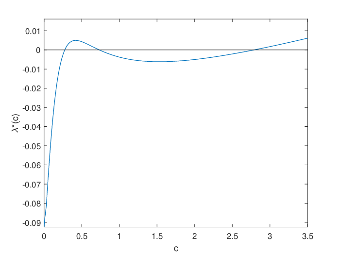
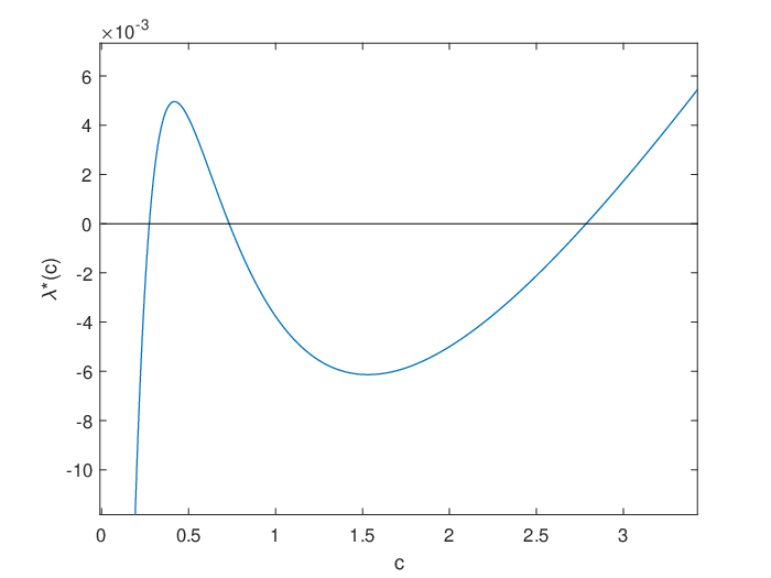
Figure 9 provides a closer look at the first of the three tipping points appearing in Figure 8. The aim is to illustrate the uniform convergence of $\mathfrak{a}_{c}$ and $\mathfrak{r}_{c}$ to the unique bounded solution at the tipping point, as proved in Theorem 4.16.

The relation $\lambda^{*}(0,p+\lambda)=\lambda^{*}(0,p)-\lambda$ (proved in Theorem 3.6(v)) and the fact that $\lambda_{*}$ is bounded (proved in Theorem 4.13(i)), show that we can modify the function $p$ in order to get examples of equations (4.1) for which no tipping occurs. For instance, replacing $p$ by $p_{1}:=p+\lambda_{*}(0)-1$ , the corresponding equations (4.1)_c are in Case C for any $c\geq 0$ : using Theorem 4.13(i), we observe that $\lambda^{*}(0,p_{1}-q_{c})=\lambda_{*}(c)-\lambda_{*}(0)+1\geq 1$ for any $c\geq 0$ ; of course, this function $p_{1}$ does not satisfy Hypothesis 4.1. For $p_{2}:=p+\sup_{c\geq 0}\lambda_{*}(c)+1$ , we are always in Case A, since $\lambda^{*}(0,p_{2}-q_{c})=\lambda_{*}(c)-\sup_{c\geq 0}\lambda_{*}(c)-1\leq-1$ . Assuming the accuracy of the representation of $\lambda_{*}$ , we can also get functions $p_{3}$ and $p_{4}$ for which the corresponding $\lambda_{*}$ takes the value 0 at a local maximum or at a local minimum, so that a punctual Case B “interrupts” Cases A or C.

We conclude by explaining the numerical evidences we have mentioned at the beginning of this subsection. We obtain them by representing solutions of (4.18). Independently of the initial time, the numerical approximation of every solution starting in an initial value greater than $2$ eventually falls onto the graph of the function $\widetilde{a}_{*}$ , which we represent in solid red in Figure 10. The analogous behavior is observed backwards in time when approximating solutions with initial value less than $-2$ , which are eventually mapped on the graph of $\widetilde{r}_{*}$ , represented in dashed blue in Figure 10. In addition, the solution corresponding to any initial pair (initial time, initial value) between the graphs of $\widetilde{a}_{*}$ and $\widetilde{r}_{*}$ falls onto the red curve as time increases and onto the blue curve as time decreases. In other words, we observe numerically that $(\widetilde{a}_{*},\widetilde{r}_{*})$ is an attractor-repeller pair for (4.18), which is our first assumption. Finally, the time of collision of solutions starting at a distance less than 5 to one of the hyperbolic solutions is never greater than 20, which is much less than $950$ and justifies the validity of our second assumption (4.19).

Conclusions and outlook

The first part of this work gives a complete mathematical description of the possible dynamical scenarios for concave scalar differential equations of the form $x^{\prime}=-x^{2}+q(t)x+p(t)$ , where $q$ and $p$ are bounded and uniformly continuous functions. The obtained results are used to study rate-induced tipping for differential equations that are asymptotically non-autonomous. Specifically, they allow to characterize the occurrence of a rate-induced tipping in terms of a non-autonomous saddle-node bifurcation for the class of differential equations

y^{\prime}=-\Big(y-\frac{2}{\pi}\,\arctan(ct)\Big)^{2}+p(t)\,,

(4.21)

where $p:\mathbb{R}\to\mathbb{R}$ is a bounded and uniformly continuous function, and $c\geq 0$ . The numerical analysis carried out in this paper shows that an intrinsically non-autonomous system subjected to a time-dependent variation of a parameter can admit more than one tipping point upon the variation of $c>0$ .

This work shades light on an important connection between rate-induced tipping and non-autonomous bifurcation theory. Moreover, it aims to prompt further studies on this subject which, in spite of its inherent complexity, appears to be the natural framework for rate-induced tipping. Natural followups include for example the following points.

•

In regard to (4.21), it seems natural to ask if $\arctan(ct)$ can be replaced by any other odd asymptotically constant function $\Gamma(ct)$ . One can show that if $\Gamma$ is also $C^{1}$ then the change of variable (4.6) is still possible. Appropriate extensions of the results are, however, far from straightforward. In fact, an in-depth analysis shows that some properties only require that $\Gamma$ is uniformly continuous and bounded (such as the continuity of $\lambda^{*}$ provided by Theorem 4.13 for example). Other properties hold if $\Gamma$ is increasing, and some of our results seem to depend also on the properties of convexity and concavity of $\arctan$ (such as the number of tipping points for example).
•

The study of analogous results for higher-order (instead of quadratic) polynomials is very interesting, but requires further significant analysis. Although the dynamical scenarios presented in this paper are still possible for some polynomials of order three or higher, different types of bifurcations or dynamical behaviors can emerge. We note that for our work, it is important that the model was globally concave and coercitive. For instance, some properties could remain valid for third-order polynomials, but important restrictions may need to be added to the equation. Moreover, it can be expected that the results will not be global in this case.
•

Alkhayuon and Ashwin [1] introduce the concept of partial and total tipping in the context of asymptotically autonomous systems whose attractors are compact sets, each given by the trajectory of an orbitally asymptotically stable solution. The current state of the art does not allow to pose the same question in the context of asymptotically nonautonomous systems. Nevertheless, a different interpretation of partial and total tipping seems plausible. If we consider our past limit system $y’=-(y+1)^{2}+p(t)$ with attractor $a(t)$ and define the time-translation of $a$ at time $s\in\mathbb{R}$ as $a_{s}(t)=a(t+s)$ , then the translated solution $a_{s}$ is not a solution of the system anymore (translation invariance only holds for autonomous systems in general), but it is a solution of the translated system $y’=-(y+1)^{2}+p_{s}(t)$ , with $p_{s}(t)=p(t+s)$ . It seems natural that the existence and number of tipping points for the family of past limit equations obtained for $\{p_{s}\mid s\in\mathbb{R}\}$ would depend on $s$ . In some cases and for some values of $c$ , the existence of separate hyperbolic solutions persists for all values of $s$ , but in other cases, this feature persists only for some values of $s$ and may fail for others, and finally it is also possible that a critical transition occurs for all values of $s$ .

Appendix A Proof of Theorem 3.5

Let $q$ and $p$ be the bounded and uniformly continuous functions of differential equation (3.11), and let $\Omega_{q,p}$ be its hull; that is, the closure in $C(\mathbb{R},\mathbb{R}\times\mathbb{R})$ of the set $\{(q,p)_{t}\,|\;t\in\mathbb{R}\}$ , where $C(\mathbb{R},\mathbb{R}\times\mathbb{R})$ is endowed with the compact-open topology and $(q,p)_{t}(s):=(q(t+s),p(t+s))$ . It is well-known that $\Omega_{q,p}$ is a compact metric space, and that the map $\sigma\colon\mathbb{R}\times\Omega_{q,p}\to\Omega_{q,p},\,(t,\omega)\mapsto\omega_{t}$ , with $\omega_{t}(s):=\omega(t+s)$ , defines a continuous flow on it (see, e.g., [31]). And it is obvious that the operator $(q_{*},p_{*})\colon\Omega_{q,p}\to\mathbb{R}\times\mathbb{R}$ , $\omega\mapsto\omega(0)$ , is continuous and satisfies $(q_{*},p_{*})(\omega_{t})=\omega(t)$ . Note that if $\omega=(\omega_{1},\omega_{2})$ then $q_{*}(\omega)=\omega_{1}(0)$ and $p_{*}(\omega)=\omega_{2}(0)$ . We will represent $\omega^{q,p}:=(q,p)\in\Omega_{q,p}$ , so that $q_{*}((\omega^{q,p})_{t})=q(t)$ and $p_{*}((\omega^{q,p})_{t})=p(t)$ . Now we can consider the family of scalar equations

x^{\prime}=-x^{2}+q_{*}(\omega_{t})\,x+p_{*}(\omega_{t})

(A.1)

for $\omega\in\Omega_{q,p}$ , which includes (3.11). Let $t\mapsto u(t,\omega,x_{0})$ represent the maximal solution of (A.1) with $u(0,\omega,x_{0})=x_{0}\in\mathbb{R}$ . The continuity of the flow on the hull, the uniqueness of solutions of initial value problems for (A.1), and standard results on continuous dependence for ordinary differential equations, ensure that

\tau\colon\mathcal{U}\subseteq\mathbb{R}\times\Omega_{q,p}\times\mathbb{R}\to\Omega_{q,p}\times\mathbb{R}\,,\quad(t,\omega,x_{0})\mapsto(\omega_{t},u(t,\omega,x_{0}))\,,

(A.2)

defines a (local) continuous flow on $\Omega_{q,p}\times\mathbb{R}$ . The set $\mathcal{U}$ is obviously composed by those points $(t,\omega,x_{0})$ for which $u(t,\omega,x_{0})$ exists. Clearly, the (scalar) flow $\tau$ is monotone with respect to its state variable; i.e., if $x_{1}<x_{2}$ , then $u(t,\omega,x_{1})<u(t,\omega,x_{2})$ as long as both solutions are defined. In addition, the flow $\tau$ is $C^{1}$ and strictly concave with respect to the state variable. The strict concavity means that

u(t,\omega,\rho\,x_{1}+(1-\rho)\,x_{2})>\rho\,u(t,\omega,x_{1})+(1-\rho)\,u(t,\omega,x_{2})

(A.3)

whenever $t>0$ , $\omega\in\Omega$ , $x_{1},x_{2}\in\mathbb{R}$ and $\rho\in(0,1)$ , and as long as all the involved terms are defined. This property can be proved as for (3.13). Taking $t<0$ reverts the sign of the inequalities. Note also that

x(t,0,x_{0})=u(t,\omega^{q,p},x_{0})\qquad\text{and}\qquad x(t,s,x_{0})=u(t-s,(\omega^{q,p})_{s},x_{0})

(A.4)

whenever the right (or left) terms of these equalities are defined.

Remark A.1.

The pair of functions $(q,p)$ (or the differential equation (3.11)) is said to be recurrent if the flow on its hull $\Omega_{q,p}$ is minimal. This is for instance the case if $q\colon\mathbb{R}\to\mathbb{R}$ and $p\colon\mathbb{R}\to\mathbb{R}$ are almost periodic functions (as deduced from the results in [12, Chapter 1], combined with [34, Proposition IV.2.3]).

Recall that Theorem 3.5 refers to the solutions $a$ and $r$ of equation (3.11) provided by Theorem 3.1, which are assumed to be globally defined and uniformly separated.

Proof of Theorem 3.5. (i) The proof of the assertions in (i) is made in six steps, making use of the flow $\tau$ defined by (A.2). We define

\delta:=\inf_{t\in\mathbb{R}}(a(t)-r(t))>0\,.

Step 1. Let us consider the family of equations (A.1). We prove that there exist globally defined and bounded functions $a_{*}\colon\Omega_{q,p}\to\mathbb{R}$ and $r_{*}\colon\Omega_{q,p}\to\mathbb{R}$ such that $u(t,\omega,x_{0})$ is globally defined and bounded if and only if $r_{*}(\omega)\leq x_{0}\leq a_{*}(\omega)$ , with $\inf_{\omega\in\Omega_{q,p}}(a_{*}(\omega)-r_{*}(\omega))\geq\delta$ , and such that

\!\!\!\!u(t,\omega,a_{*}(\omega))=a_{*}(\omega_{t})\;\text{ and }\;u(t,\omega,r_{*}(\omega))=r_{*}(\omega_{t})\;\text{ for $\omega\in\Omega_{q,p}$ and $t\in\mathbb{R}$}\,.

(A.5)

Let us define

\mathcal{B}_{\omega}:=\{x_{0}\in\mathbb{R}\,|\;u(t,\omega,x_{0})\;\text{is globally defined and bounded}\}\,.

We fix $m>0$ such that $-m^{2}+q_{*}(\omega)\,m+p_{*}(\omega)<-1$ for any $\omega\in\Omega_{q,p}$ . We check that $\mathcal{B}_{\omega}$ is nonempty and contained in $[-m,m]$ for any $\omega\in\Omega_{q,p}$ . Let us take any $\omega^{0}\in\Omega_{q,p}$ , choose $(t_{n})$ such that $\omega^{0}=\lim_{n\to\infty}(\omega^{q,p})_{t_{n}}$ , and assume without restriction that there exist $a^{0}=\lim_{n\to\infty}a(t_{n})$ and $r^{0}=\lim_{n\to\infty}r(t_{n})$ . Then,

	$\displaystyle u(t,\omega^{0},a^{0})$	$\displaystyle=\lim_{n\to\infty}u(t,(\omega^{q,p})_{t_{n}},a(t_{n}))=\lim_{n\to\infty}u(t,u(t_{n},\omega^{q,p},a(0)))$
		$\displaystyle=\lim_{n\to\infty}a(t+t_{n})\,,$

so that the solution $u(t,\omega^{0},a^{0})$ is bounded on its domain and hence globally defined. This ensures that $a^{0}\in\mathcal{B}_{\omega^{0}}$ . Similarly, $r^{0}\in\mathcal{B}_{\omega^{0}}$ . Now we define $a_{*}(\omega^{0}):=\sup\mathcal{B}_{\omega^{0}}$ and $r_{*}(\omega^{0}):=\inf\mathcal{B}_{\omega^{0}}$ . Theorem 3.1(i)&(ii) ensure that $a_{*}(\omega^{0})$ and $r_{*}(\omega^{0})$ belong to $[-m,m]$ : they are the functions provided by that theorem for the equation $x^{\prime}=-x^{2}+p_{*}((\omega^{0})_{t})$ evaluated at $t=0$ , and the corresponding condition (3.2) is satisfied. In addition, $a_{*}(\omega^{0})-r_{*}(\omega^{0})\geq a^{0}-r^{0}=\lim_{n\to\infty}(a(t_{n})-r(t_{n}))\geq\delta$ . To complete Step 1, note that

a_{*}((\omega^{q,p})_{t})=a(t)\quad\text{and}\quad r_{*}((\omega^{q,p})_{t})=r(t)\quad\text{for all $t\in\mathbb{R}$}\,,

(A.6)

that the analogous equalities hold for any $\omega\in\Omega$ , and that they guarantee (A.5).

Step 2. We prove that, if $\mathcal{M}\subset\Omega_{q,p}$ is a minimal set, then the maps $\mathcal{M}\to\mathbb{R}\,,\;\omega\mapsto a_{*}(\omega)$ , and $\mathcal{M}\to\mathbb{R}\,,\;\omega\mapsto r_{*}(\omega)$ , are continuous; and that given $\rho>0$ , there exist $\beta_{\mathcal{M}}>0$ and $k_{\rho,\mathcal{M}}\geq 1$ such that

\begin{split}&|a_{*}(\omega_{t})-u(t,\omega,x_{0})|\leq k_{\rho,\mathcal{M}}e^{-\beta_{\mathcal{M}}t}|a_{*}(\omega)-x_{0}|\\ &\qquad\qquad\qquad\quad\text{for $t\geq 0$, $\omega\in\mathcal{M}$ and $x_{0}\geq r_{*}(\omega)+\rho$}\,,\\ &|r_{*}(\omega_{t})-u(t,\omega,x_{0})|\leq k_{\rho,\mathcal{M}}e^{\beta_{\mathcal{M}}t}|r_{*}(\omega)-x_{0}|\\ &\qquad\qquad\qquad\quad\text{for $t\leq 0$, $\omega\in\mathcal{M}$ and $x_{0}\leq a_{*}(\omega)-\rho$}\,.\end{split}

(A.7)

For the map $a_{*}$ , the assertions follow from the strict concavity of the flow $\tau$ defined by (A.2), and [24, Theorems 3.12 and 3.8(iv)]. To prove the assertions concerning $r_{*}$ , we proceed as follows:

-

We first define a new flow on the hull $\Omega_{q,p}$ by reversion of time: $\sigma^{-}(t,\omega)=\omega_{-t}$ .

We consider the family of equations $z^{\prime}=-z^{2}-q_{*}(\omega_{-t})\,z+p_{*}(\omega_{-t})$ , which induces the new flow

\qquad\tau^{-}\colon\mathcal{U}\subseteq\mathbb{R}\times\Omega_{q,p}\times\mathbb{R}\to\Omega_{q,p}\times\mathbb{R}\,,\quad(t,\omega,z_{0})\mapsto(\omega_{-t},w(t,\omega,z_{0}))\,,

and check that $w(t,\omega,z_{0})=-u(-t,\omega,-z_{0})$ . Consequently,

\mathcal{B}_{\omega}^{-}:=\{z_{0}\,|\;{-}a_{*}(\omega)\leq z_{0}\leq-r_{*}(\omega)\}

are the sets of initial conditions giving rise to bounded solutions.

We observe that the differential equation corresponding to $\omega^{q,p}$ is given by $z^{\prime}=-z^{2}-q(-t)\,z+p(-t)$ , and hence that the roles of the solutions $\bar{a}(t)=-a(-t)$ and $\bar{r}(t)=-r(-t)$ of this differential equation correspond to the roles played by $r$ and $a$ for the original differential equation, respectively; and we have $\inf_{t\in\mathbb{R}}(\bar{r}(t)-\bar{a}(t))=\delta>0$ . Therefore, the results obtained so far for $a$ and $a_{*}$ apply to $\bar{r}$ and $-r_{*}$ , leading us to conclude that given $\rho>0$ , there exist $\beta_{\mathcal{M}}>0$ and $k_{\rho,\mathcal{M}}\geq 1$ such that

\begin{split}&\qquad|{-}r_{*}(\omega_{-t})-w(t,\omega,z_{0})|\leq k_{\rho,\mathcal{M}}e^{-\beta_{\mathcal{M}}t}|{-}r_{*}(\omega)-z_{0}|\\ &\qquad\qquad\qquad\qquad\quad\text{for $t\geq 0$, $\omega\in\mathcal{M}$ and $z_{0}\geq-a_{*}(\omega)+\rho$}\,,\end{split}

This fact and the previous equalities prove the second assertion in (A.7), which completes this step.

Step 3. We prove that any point $\omega^{1}$ belonging to a minimal subset of $\Omega_{q,p}$ is a continuity point for $a_{*}\colon\Omega_{q,p}\to\mathbb{R}$ and $r_{*}\colon\Omega_{q,p}\to\mathbb{R}$ .

We take a sequence $(\omega_{n})$ in $\Omega_{q,p}$ with limit $\omega^{1}$ . We check that $a_{*}(\omega^{1})=\lim_{n\to\infty}a_{*}(\omega_{n})$ and $r_{*}(\omega^{1})=\lim_{n\to\infty}r_{*}(\omega_{n})$ . Note that it is enough to check the following: if for a subsequence $(\omega_{m})$ , there exist $a^{1}:=\lim_{m\to\infty}a_{*}(\omega_{m})$ and $r^{1}:=\lim_{m\to\infty}r_{*}(\omega_{m})$ , then $a^{1}=a_{*}(\omega^{1})$ and $r^{1}=r_{*}(\omega^{1})$ .

So that let us take such a subsequence. It follows from (A.5) that $u(s,\omega^{1}\!,a^{1})=\lim_{m\to\infty}a_{*}((\omega_{m})_{s})$ and $u(s,\omega^{1}\!,r^{1})=\lim_{m\to\infty}r_{*}((\omega_{m})_{s})$ for $s\in\mathbb{R}$ , which, as seen in Step 1, ensures that $u(s,\omega^{1}\!,a^{1})$ and $u(s,\omega^{1}\!,r^{1})$ are bounded solutions. Hence, $r_{*}(\omega^{1})\leq r^{1}\leq a^{1}\leq a_{*}(\omega^{1})$ and, for any $s\in\mathbb{R}$ ,

\begin{split}u(s,\omega^{1}\!,a^{1})-r_{*}((\omega^{1})_{s})&=u(s,\omega^{1}\!,a^{1})-u(s,\omega^{1}\!,r_{*}(\omega^{1}))\geq u(s,\omega^{1}\!,a^{1})-u(s,\omega^{1}\!,r^{1})\\ &=\lim_{m\to\infty}\big(a_{*}((\omega_{m})_{s})-r_{*}((\omega_{m})_{s})\big)\geq\delta\,.\end{split}

According to Step 2, there exist $\beta_{\mathcal{M}}>0$ and $k_{\delta,\mathcal{M}}\geq 1$ such that

|a_{*}((\omega^{1})_{t})-u(t-s,(\omega^{1})_{s},u(s,\omega^{1}\!,a^{1}))|\leq k_{\delta,\mathcal{M}}\,e^{-\beta_{\mathcal{M}}(t-s)}|a_{*}((\omega^{1})_{s})-u(s,\omega^{1}\!,a^{1})|

if $t\geq s$ . Therefore, taking $t=0$ ,

|a_{*}(\omega^{1})-a^{1}|\leq k_{\delta,\mathcal{M}}\,e^{\beta_{\mathcal{M}}s}|a_{*}((\omega^{1})_{s})-u(s,\omega^{1}\!,a^{1})|

for $s\leq 0$ . Since $\sup_{s\in\mathbb{R}}|a_{*}((\omega^{1})_{s})-u(s,\omega^{1}\!,a^{1})|<\infty$ , we conclude that $a_{*}(\omega^{1})=a^{1}$ , as asserted. The proof of $r^{1}=r_{*}(\omega^{1})$ can be done in an analogous way.

Step 4. We prove that the maps $a_{*}$ and $r_{*}$ are continuous on $\Omega_{q,p}$ .

We take $\omega^{2}\in\Omega_{q,p}$ and a sequence $(\omega_{n})$ in $\Omega_{q,p}$ with limit $\omega^{2}$ . We will check that $a_{*}(\omega^{2})=\lim_{n\to\infty}a_{*}(\omega_{n})$ and $r_{*}(\omega^{2})=\lim_{n\to\infty}r_{*}(\omega_{n})$ . Again, we will check that if for a subsequence $(\omega_{m})$ , there exist $a^{2}:=\lim_{m\to\infty}a_{*}(\omega_{m})$ and $r^{2}:=\lim_{m\to\infty}r_{*}(\omega_{m})$ , then $a^{2}=a_{*}(\omega^{2})$ and $r^{2}=r_{*}(\omega^{2})$ .

The hypothesis on uniform separation ensures that $r^{2}\leq a^{2}-\delta$ . As seen in Step 2, the solutions $u(s,\omega^{2}\!,a^{2})$ and $u(s,\omega^{2}\!,r^{2})$ are bounded, and hence $r_{*}(\omega^{2})\leq r^{2}<a^{2}\leq a_{*}(\omega^{2})$ . This and (A.5) ensure that, for any $s\in\mathbb{R}$ ,

\begin{split}a_{*}((\omega^{2})_{s})-u(s,\omega^{2}\!,r^{2})&=u(s,\omega^{2}\!,a_{*}(\omega^{2}))-u(s,\omega^{2}\!,r^{2})\geq u(s,\omega^{2}\!,a^{2})-u(s,\omega^{2}\!,r^{2})\\ &=\lim_{m\to\infty}a_{*}((\omega_{m})_{s})-r_{*}((\omega_{m})_{s})\geq\delta\,.\end{split}

Now let us assume for contradiction that $r^{2}>r_{*}(\omega^{2})$ , and look for $\rho\in(0,1)$ such that $r^{2}=\rho\,a_{*}(\omega^{2})+(1-\rho)\,r_{*}(\omega^{2})$ . Then, the concavity of the flow $\tau$ ensures that $u(s,\omega^{2},r^{2})\geq\rho\,a_{*}((\omega^{2})_{s})+(1-\rho)\,r_{*}((\omega^{2})_{s})$ for any $s\geq 0$ (see (A.3)), and hence,

u(s,\omega^{2},r^{2})-r_{*}((\omega^{2})_{s})\geq\rho\,\big(a_{*}((\omega^{2})_{s})-r_{*}((\omega^{2})_{s})\big)\geq\rho\,\delta

for any $s\geq 0$ . Let us take a point $(\omega^{1},x^{1})$ in a minimal set contained in the omega-limit set of $(\omega^{2},r^{2})$ for the flow $\tau$ , and note that $\omega^{1}$ belongs to a minimal subset $\mathcal{M}$ of $\Omega_{q,p}$ for the flow on the hull. It follows easily from the previous inequalities, the continuity of $\tau$ , and the continuity of $r_{*}$ and $a_{*}$ at $\omega^{1}\in\mathcal{M}$ established on Step 4 that

r_{*}((\omega^{1})_{t})+\rho\,\delta\leq u(t,\omega^{1},x^{1})\leq a_{*}((\omega^{1})_{t})-\delta

for any $t\geq 0$ . But this contradicts the information regarding the asymptotic behavior of the solutions provided by Step 2: $\lim_{t\to\infty}(a_{*}((\omega^{1})_{t})-u(t,\omega^{1},x^{1}))=0$ , since $x^{1}\geq r_{*}(\omega^{1})+\rho\,\delta$ . This contradiction shows that $r^{2}=r_{*}(\omega^{2})$ .

The proof for $a_{*}$ can be done similarly, now working for negative values of time and for the alpha-limit set of $(\omega^{2},a^{2})$ . This completes Step 4.

Step 5. We prove the absence of non-trivial bounded solutions for all the linear differential equations

y^{\prime}=(2\,a_{*}(\omega_{t})-q_{*}(\omega_{t}))\,y\quad\text{and}\quad y^{\prime}=(2\,r_{*}(\omega_{t})-q_{*}(\omega_{t}))\,y\,.

(A.8)

Let us work with $a_{*}$ , assuming for contradiction the existence of $\omega^{4}$ such that

\sup_{t\in\mathbb{R}}\left(\exp\int_{0}^{t}(2\,a_{*}((\omega^{4})_{l})-q_{*}((\omega^{4})_{l}))\,\mathrm{d}l\right)=:\kappa<\infty\,,

and let us take any $x^{4}\in(r_{*}(\omega^{4}),a_{*}(\omega^{4}))$ . By repeating the argument leading to (3.14), we get

\begin{split}a_{*}((\omega^{4})_{t})-u(t,\omega^{4},x^{4})&\geq(a_{*}(\omega^{4})-x^{4})\exp\int_{0}^{t}(-2\,a_{*}((\omega^{4})_{l})+q_{*}((\omega^{4})_{l}))\,\mathrm{d}l\\ &\geq(1/\kappa)(a_{*}(\omega^{4})-x^{4})=:\delta_{3}>0\end{split}

for any $t>0$ . By reasoning as in Step 4, we prove that there exists $\rho\in(0,1)$ with

u(t,\omega^{4},x^{4})-r_{*}((\omega^{4})_{t})\geq\rho\,\delta

for any $t\geq 0$ , and we reach the required contradiction by repeating the final argument of Step 4.

Step 6. We prove that the solutions $a_{*}(\omega_{t})$ and $r_{*}(\omega_{t})$ of equation (A.1)_ω (see (A.5)) are hyperbolic, which combined with (A.6) proves (i).

We first take a point $\omega$ in a minimal subset $\mathcal{M}$ of $\Omega_{q,p}$ , and $x_{0}\in[a_{*}(\omega),r_{*}(\omega)]$ . By repeating the argument leading to (3.14) and (3.15), and using the information from Step 2, we find

\begin{split}&\exp\int_{0}^{t}(-2\,a_{*}(\omega_{l})+q_{*}(\omega_{l}))\,\mathrm{d}l\leq\frac{a_{*}(\omega_{t})-u(t,\omega,x_{0})}{a_{*}(\omega)-x_{0}}\leq k_{\rho,\mathcal{M}}e^{-\beta_{\mathcal{M}}t}\quad\text{if $t\geq 0$}\,,\\ &\exp\int_{0}^{t}(-2\,r_{*}(\omega_{l})+q_{*}(\omega_{l}))\,\mathrm{d}l\leq\frac{u(t,\omega,x_{0})-r_{*}(\omega_{t})}{x_{0}-r_{*}(\omega)}\leq k_{\rho,\mathcal{M}}e^{\beta_{\mathcal{M}}t}\quad\text{if $t\leq 0$}\,.\end{split}

It follows easily that the equations

y^{\prime}=(-2\,a_{*}(\omega_{t})+q_{*}(\omega_{t}))\,y\quad\text{and}\quad y^{\prime}=(-2\,r_{*}(\omega_{t})+q_{*}(\omega_{t}))\,y

(A.9)

have an exponential dichotomy for each element $\omega$ of any minimal subset $\mathcal{M}$ of $\Omega_{q,p}$ , where the first ones are of Hurwitz type at $+\infty$ and the second ones are of Hurwitz type at $-\infty$ . Therefore, also the equations (A.8) have an exponential dichotomy for each element $\omega$ of each minimal subset $\mathcal{M}$ of $\Omega_{q,p}$ , where the first ones are of Hurwitz type at $-\infty$ and the second ones are of Hurwitz type at $+\infty$ , see e.g. [19, Proposition 1.73 and Theorem 1.60]. This fact combined with the absence of bounded solutions established in Step 5 guarantees the exponential dichotomy of the equations (A.8) for any $\omega\in\Omega_{q,p}$ , see [28, Theorem 2], and applying [19, Proposition 1.73 and Theorem 1.60] again ensures that every differential equation in (A.9) has an exponential dichotomy, which proves our assertion.

(ii) Let us concentrate on the hyperbolic solution $a$ first. We fix a dichotomy constant pair for $a$ (see Section 2), and now check that $(k_{a},\beta_{a})$ is a dichotomy constant pair for the hyperbolic solution $a_{*}(\omega_{t})$ of equation (A.1)_ω (see (A.5)), for any $\omega\in\Omega_{q,p}$ . So, we take $\omega\in\Omega_{q,p}$ and obtain it as limit $\omega=\lim_{n\to\infty}(\omega^{q,p})_{t_{n}}$ for a suitable sequence $(t_{n})$ . The continuity of the flow on $\Omega_{q,p}$ , the continuity of $a_{*}$ (proved in Step 4 of (i)) and the first equality in (A.6) show that

\begin{split}&\exp\int_{s}^{t}(-2\,a_{*}(\omega_{l})+q_{*}(\omega_{l}))\,\mathrm{d}l=\lim_{n\to\infty}\exp\int_{s}^{t}(-2\,a(t_{n}+l)+q(t_{n}+l))\,\mathrm{d}l\\ &\qquad\qquad=\lim_{n\to\infty}\exp\int_{s+t_{n}}^{t+t_{n}}(-2\,a(l)+q(l))\,\mathrm{d}l\leq k_{a}\,e^{-\beta_{a}(t-s)}\quad\text{if $t\geq s$}\,,\end{split}

which proves the assertion.

Let us fix $\bar{\beta}_{a}\in(0,\beta_{a})$ . Now we reason as in the proof of Proposition 3.3. By reviewing the proof of [14, Theorem III.2.4], we conclude that there exists $\rho>0$ (which depends just on the choice of $\bar{\beta}_{a}$ ) such that

\begin{split}&|a_{*}(\omega_{t})-u(t,\omega,x_{0})|\leq k_{a}e^{-\bar{\beta}_{a}t}|a_{*}(\omega)-x_{0}|\\ &\qquad\qquad\qquad\quad\text{for $\,t\geq 0\,$, $\,\omega\in\Omega_{q,p}\,$ and $\,|x_{0}-a_{*}(\omega)|<\rho$}\,.\end{split}

(A.10)

And we also check (as in Proposition 3.3) that

\begin{split}&|a_{*}(\omega_{t})-u(t,\omega,x_{0})|\leq k_{a}\,e^{-\beta_{a}\,t}\,|a_{*}(\omega)-x_{0}|\\ &\qquad\qquad\qquad\quad\text{for $\,t\geq 0\,$, $\,\omega\in\Omega_{q,p}\,$ and $\,x_{0}\geq a_{*}(\omega)$}\,.\end{split}

(A.11)

Now we fix $\varepsilon>0$ and check that for each $\omega^{0}\in\Omega_{q,p}$ , there exists a time $t_{\omega^{\!0}}$ such that

|u(t_{\omega^{\!0}},\omega^{0},r_{*}(\omega^{0})+\varepsilon)-a_{*}((\omega^{0})_{t_{\omega^{\!0}}})|<\rho\,.

If $r(\omega^{0})+\varepsilon\geq a_{*}(\omega^{0})-\rho$ , this inequality follows from (A.10) and (A.11). Assume hence that $r_{*}(\omega^{0})+\varepsilon\leq a_{*}(\omega^{0})-\rho$ . The non-existence of $t_{\omega^{0}}$ would ensure that $a_{*}((\omega^{0})_{t})-u(t,\omega^{0},r_{*}(\omega^{0})+\varepsilon)\geq\rho$ for every $t\geq 0$ . In that case, we take $(\omega^{1},x^{1})$ in a minimal set contained in the omega-limit set of $(\omega^{0},r_{*}(\omega^{0})+\varepsilon)$ and conclude from the continuity of $\tau$ and that of $a_{*}$ (proved in (i)) that $a_{*}((\omega^{1})_{t})-u(t,\omega^{1},r_{*}(\omega^{1})+\varepsilon)\geq\rho$ for every $t\geq 0$ . But this contradicts the first inequality in (A.7), so that our assertion is proved. We point out that $t_{\omega^{\!0}}$ depends on $\omega^{0}$ , $\varepsilon$ and $\rho$ , and hence on $\omega^{0}$ , $\varepsilon$ and $\bar{\beta}_{a}$ .

Note now that for any $\omega^{0}\in\Omega_{q,p}$ there exists an open neighborhood $\mathcal{U}_{\omega^{0}}$ such that $|u(t_{\omega^{\!0}},\omega,r_{*}(\omega)+\varepsilon)-a_{*}(\omega_{t_{\omega^{\!0}}})|<\rho$ for any $\omega\in\mathcal{U}_{\omega^{0}}$ . Therefore the compactness of $\Omega_{q,p}$ provides a finite number of times $t_{1},\ldots,t_{n}$ such that for any $\omega\in\Omega_{q,p}$ there exists $j=j(\omega)\in\{1,\ldots,n\}$ with $|u(t_{j},\omega,r_{*}(\omega)+\varepsilon)-a_{*}(\omega_{t_{j}})|<\rho$ . We define $T:=\max(t_{1},\ldots,t_{n})$ and note that $T$ depends on the choices of $\varepsilon$ and $\bar{\beta}_{a}$ .

Let us now fix $\omega\in\Omega_{q,p}$ and $x_{0}\geq r_{*}(\omega)+\varepsilon$ . If $x_{0}\geq a_{*}(\omega)-\rho$ , then (A.10) and (A.11) ensure that

|a_{*}(\omega_{t})-u(t,\omega,x_{0})|\leq k_{a}e^{-\bar{\beta}_{a}t}|a_{*}(\omega)-x_{0}|\quad\text{if $t\geq 0$}\,.

(A.12)

So that we assume that $x_{0}\in[r_{*}(\omega)+\varepsilon,a_{*}(\omega)-\rho]$ . We choose $j=j(\omega)$ as above, and note that the monotonicity of the flow ensures that $|u(t_{j},\omega,x_{0})-a_{*}(\omega_{t_{j}})|<\rho$ . Therefore, if $t\geq T$ (and hence $t\geq t_{j}$ ),

\begin{split}|a_{*}(\omega_{t})-u(t,\omega,x_{0})|&=|a_{*}((\omega_{t_{j}})_{(t-t_{j})})-u(t-t_{j},\omega_{t_{j}},u(t_{j},\omega,x_{0}))|\\ &\leq k_{a}\,e^{-\bar{\beta}_{a}(t-t_{j})}|a_{*}(\omega_{t_{j}})-u(t_{j},\omega,x_{0})|\\ &\leq k_{a}\,e^{-\bar{\beta}_{a}t}e^{\bar{\beta}_{a}T}\rho\leq k_{a}\,e^{\bar{\beta}_{a}T}e^{-\bar{\beta}_{a}t}|a_{*}(\omega)-x_{0}|\,.\end{split}

(A.13)

Now we define

\kappa:=\sup_{t\in[0,T],\;\omega\in\Omega,\;x_{0}\in[r_{*}(\omega)+\varepsilon,a_{*}(\omega)-\rho]}\frac{|a_{*}(\omega_{t})-u(t,\omega,x_{0})|}{e^{-\bar{\beta}t}|a_{*}(\omega)-x_{0}|}\,,

which is finite since the function on the right is a continuous map on a compact metric space. While being independent of $\omega$ and $x_{0}$ , the quantity $\kappa$ depends on $\varepsilon$ and on $\bar{\beta}_{a}$ (as $\rho)$ . Then, if $t\in[0,T]$ ,

\begin{split}|a_{*}(\omega_{t})-u(t,\omega,x_{0})|\leq\kappa\,e^{-\bar{\beta}_{a}t}|a_{*}(\omega)-x_{0}|\,.\end{split}

(A.14)

Summing up, assertions (A.12), (A.13) and (A.14) lead to

\begin{split}&|a_{*}(\omega_{t})-u(t,\omega,x_{0})|\leq k_{a,\varepsilon}\,e^{-\bar{\beta}_{a}t}|a_{*}(\omega)-x_{0}|\\ &\qquad\qquad\qquad\quad\text{for $t\geq 0$, $\omega\in\Omega_{q,p}$ and $x_{0}\geq r_{*}(\omega)+\varepsilon$}\,,\end{split}

where $k_{a,\varepsilon}:=\max(k_{a},k_{a}\,e^{\bar{\beta}_{a}T},\kappa)$ . Note that $k_{a,\varepsilon}$ depends on $\varepsilon$ and $\bar{\beta}_{a}$ , but neither on $\omega$ nor on $x_{0}$ .

The first statement concerning $a$ in (ii) follows from the previous assertion and the equalities (A.6) and (A.4), and the second one from these equalities and (A.11).

In order to prove the result for $r$ , we make the change of variable $z(t)=-x(-t)$ , which transforms the equation $x^{\prime}=-x^{2}+q(t)\,x+p(t)$ in $z^{\prime}=-z^{2}-q(-t)\,z+p(-t)$ , with solutions $z(t,s,z_{0})=-x(-t,-s,-z_{0})$ . We apply the results so far proved to the transformed equation, for which the functions $\bar{r}(t)=-r(-t)$ and $\bar{a}(t)=-a(-t)$ play the same roles as $a$ and $r$ for the initial one, respectively. From here the proof is easily completed: see the end of the proof of Step 2 in (i).

(iii) Let us check that $a$ and $r$ are uniformly separated, reasoning by contradiction: it is easy to deduce from (i) that otherwise there exist $k\geq 1$ and $s_{0}$ such that $\exp\int_{s_{0}}^{t}(-2\,r(l)+q(l))\,\mathrm{d}l\leq k\,e^{-(\beta_{a}/2)(t-s_{0})}$ whenever $t\geq s_{0}$ . But this implies that the solutions $z(t,s_{0},z_{0})$ of the linearized equation $z^{\prime}=(-2\,r(t)+q(t))\,z$ tend to $0$ as $t\to\infty$ , which is impossible, see the comments after the definition of hyperbolicity in Section 2.

Let $b$ be a bounded solution that is different from $a$ and $r$ , which implies $a<b<r$ . Then, (ii) ensures that $\lim_{t\to\infty}|a(t)-b(t)|=0$ and $\lim_{t\to-\infty}|r(t)-b(t)|=0$ . Therefore, $a$ and $r$ are the unique bounded and uniformly separated solutions. As above, the same property shows that, for the equation $z^{\prime}=(-2\,b(t)+q(t))\,z$ , there coexist solutions bounded for $t\to\infty$ and solutions bounded for $t\to-\infty$ , which precludes the hyperbolicity of $b$ (see Section 2). The proof is complete. $\Box$

Acknowledgments

We thank two anonymous referees for their comments and suggestions, which have been included in the current version of the paper.

References

[1] H.M. Alkhayoun, P. Ashwin, Rate-induced tipping from periodic attractors: partial tipping and connecting orbits, Chaos 28 (3) (2018), 033608, 11 pp.
[2] H.M. Alkhayoun, P. Ashwin, L.C. Jackson, C. Quinn,R.A. Wood, Basin bifurcations, oscillatory instability and rate-induced thresholds for Atlantic meridional overturning circulation in a global oceanic box model, Proc. R. Soc. A 475 (2225) (2019), 20190051.
[3] A.I. Alonso, R. Obaya, The structure of the bounded trajectories set of a scalar convex differential equation, Proc. Roy. Soc. Edinburgh 133 A (2003), 237–263.
[4] A.I. Alonso, R. Obaya, R. Ortega, Differential equations with limit-periodic forcings, Proc. Amer. Math. Soc. 131 (3) (2002), 851-–857.
[5] V. Anagnostopoulou, T. Jäger, Nonautonomous saddle-node bifurcations: Random and deterministic forcing, J. Differential Equations 253 (2) (2012), 379–399.
[6] P. Ashwin, C. Perryman, S. Wieczorek, Parameter shifts for nonautonomous systems in low dimension: bifurcation and rate-induced tipping, Nonlinearity 30 (6) (2017), 2185–2210.
[7] P. Ashwin, S. Wieczorek, R. Vitolo, P. Cox, Tipping points in open systems: bifurcation, noise-induced and rate-dependent examples in the climate system, Phil. Trans. R. Soc. A 370 (2012), 1166–1184.
[8] G. Carigi, Rate-induced tipping in nonautonomous dynamical systems with bounded noise, MRes Thesis, University of Reading, 2017.
[9] A. Carvalho, J. Langa, J. Robinson, Attractors for Infinite-dimensional Non-autonomous Dynamical Systems, Appl. Math. Sci. 182, Springer, 2013.
[10] W.A. Coppel, Disconjugacy, Lecture Notes in Math. 220, Springer-Verlag, Berlin, Heidelberg, New York, 1971.
[11] W.A. Coppel, Dichotomies in Stability Theory, Lecture Notes in Math. 629, Springer-Verlag, Berlin, Heidelberg, New York, 1978.
[12] A.M. Fink, Almost Periodic Differential Equations, Lecture Notes in Math. 377, Springer-Verlag, Berlin, Heidelberg, New York, 1974.
[13] G. Fuhrmann, Non-smooth saddle-node bifurcations III: Strange attractors in continuous time, J. Differential Equations 261 (3) (2016), 2109–2140.
[14] J.K. Hale Ordinary Differential Equations, Wiley-Interscience, New York, 1969.
[15] M. Hartl, Non-autonomous Random Dynamical Systems: Stochastic Approximation and Rate-Induced Tipping, PhD Thesis, Imperial College London, 2019.
[16] A.v. Hill, Excitation and accommodation in nerve, Proc. R. Soc. B 119 (814) (1936), 305–355.
[17] T. Kato, On the Adiabatic Theorem of Quantum Mechanics, J. Phys. Soc. Jpn. 5 (6) (1950), 435–439.
[18] P. Kloeden, M. Rasmussen, Nonautonomous Dynamical Systems, Mathematical Surveys and Monographs, Amer. Math. Soc., 2011.
[19] R. Johnson, R. Obaya, S. Novo, C. Núñez, R. Fabbri, Nonautonomous Linear Hamiltonian Systems: Oscillation, Spectral Theory and Control Developments in Mathematics 36, Springer, 2016
[20] À. Jorba, C. Núñez, R. Obaya, J.C. Tatjer, Old and new results on Strange Nonchaotic Attractors, Int. J. Bifurcation Chaos, 17 (11) (2007), 3895–3928.
[21] V.M. Millions̆c̆ikov, Proof of the existence of irregular systems of linear differential equations with almost periodic coefficients, Differ. Uravn. 4 (3) (1968), 391–396.
[22] V.M. Millions̆c̆ikov, Proof of the existence of irregular systems of linear differential equations with quasi periodic coefficients, Differ. Uravn. 5 (11) (1969), 1979–1983.
[23] C. Núñez, R. Obaya, A nonautonomus bifurcation theory for deterministic scalar differential equations, Discrete Contin. Dynam. Systems, 9 (3&4) (2008), 701–730.
[24] C. Núñez, R. Obaya, A.M. Sanz, Minimal sets in monotone and concave skew-product semiflows I: a general theory, J. Differential Equations 252 (2012), 5492–5517.
[25] C. Núñez, R. Obaya, A.M. Sanz, Minimal sets in monotone and concave skew-product semiflows II: two-dimensional systems of differential equations, J. Differential Equations 252 (2012), 3575–3607.
[26] C. Pötzsche, Nonautonomous continuation of bounded solutions, Commun. Pure Appl. Anal. 10 (3) (2011), 937–961.
[27] M. Rasmussen, Attractivity and bifurcation for nonautonomous dynamical systems, Lecture Notes in Math. 1907, Springer-Verlag, Berlin, 2007.
[28] R.J. Sacker, G.R. Sell, Existence of dichotomies and invariant splittings for linear differential systems II, J. Differential Equations 22 (1976), 478–496.
[29] M. Scheffer, Critical Transitions in Nature and Society, Princeton University Press, 2009.
[30] M. Scheffer, E.H. Van Nes, M. Holmgren, T. Hughes, Pulse-driven loss of top-down control: the critical-rate hypothesis, Ecosystems 11 (2008), 226–237.
[31] G.R. Sell, Topological Dynamics and Differential Equations, Van Nostrand Reinhold, London, 1971.
[32] A. Vanselow, S. Wieczorek, U. Feudel, When very slow is too fast-collapse of a predator-prey system, J. Theor. Biol. 479 (2019), 64–72.
[33] R.E. Vinograd, A problem suggested by N.P. Erugin, Differ. Uravn. 11 (4) (1975), 632–638.
[34] J. de Vries, Elements of Topological Dynamics, Kluwer Academic Publishers, Dordrecht, 1993.
[35] S. Wieczorek, P. Ashwin, C.M. Luke, P.M. Cox, Excitability in ramped systems: the compost-bomb instability, Proc. R. Soc. A 467 (2011), 1243–1269.
[36] S. Wieczorek, C. Xie, C.K.R.T. Jones, Compactification for asymptotically autonomous dynamical systems: theory, applications and invariant manifolds, Preprint (2020).
[37] C. Xie, Rate-Induced Critical Transitions, PhD Thesis, University College Cork, 2020.

Abstract.

Key words and phrases:

2010 Mathematics Subject Classification

1. Introduction

2. Some notions on nonautonomous differential equations and flows

3. The dynamics of the concave scalar equation x′=−x2+q⁡(t)​x+p⁡(t)x^{\prime}=-x^{2}+q(t)\,x+p(t)

3.1. Some facts on the coercitive scalar equation x′=h⁡(t,x)x^{\prime}=h(t,x)

Theorem 3.1.

Proof.

3.2. Hyperbolic solutions for x′=−x2+q⁡(t)​x+p⁡(t)x^{\prime}=-x^{2}+q(t)\,x+p(t).

Proposition 3.2.

Proof.

Proposition 3.3.

Proof.

Definition 3.4.

Theorem 3.5.

3.3. One-parametric variation of the global dynamics.

Theorem 3.6.

Proof.

Corollary 3.7.

Proof.

Remarks 3.8.

4. Rate-induced tipping

Hypothesis 4.1.

4.1. Global dynamics: the main results

Definition 4.2.

Theorem 4.3.

Theorem 4.4.

Theorem 4.5.

Theorem 4.6.

Remark 4.7.

4.2. Proofs of the main results.

Theorem 4.8.

Proof.

Theorem 4.9.

Proof.

Proposition 4.10.

Proof.

Remarks 4.11.

Proposition 4.12.

Proof.

4.3. The bifurcation curve λ∗\lambda_{*} and rate-induced tipping

Theorem 4.13.

Proof.

Remark 4.14.

Proposition 4.15.

Theorem 4.16.

Proof.

4.4. Numerical simulations

Conclusions and outlook

Appendix A Proof of Theorem 3.5

Remark A.1.

Acknowledgments

References

3. The dynamics of the concave scalar equation $x^{\prime}=-x^{2}+q(t)\,x+p(t)$

3.1. Some facts on the coercitive scalar equation $x^{\prime}=h(t,x)$

3.2. Hyperbolic solutions for $x^{\prime}=-x^{2}+q(t)\,x+p(t)$ .

4.3. The bifurcation curve $\lambda_{*}$ and rate-induced tipping