Hypothesis Testing of One Sample Mean Vector in Distributed Frameworks

Since data are stored in $k$ different machines, we denote by $S_{l}$ the set of indices of the observations on the $l$-th machine, that is, $S_{l}=\{i:X_{i}$ is stored in the $l$-th machine$\}$, $l=1,\cdots,k$. Let $n_{l}=|S_{l}|$, the sample size on the $l$-th machine. In the distributed framework, constructing the centralized test statistic is still feasible by transmitting some matrices of size $p$ by $p$, as shown in Algorithm 1.

Suppose that $\{X_{i}\}_{i=1}^{n}$ are $i.i.d.$ random variables following $N_{p}(\mbox{\boldmath{$\mu$}},\Sigma)$. Under $H_{0}$, according to the relationship between Hotelling $T^{2}$ distribution and the $F$-distribution, we have

where $F(p,n-p)$ denotes the $F$-distribution with the degrees of freedom $p$ and $n-p$. Given the significant level $\alpha\in(0,1)$, the rejection region for Hotelling $T^{2}$ test is denoted as

where $F_{1-\alpha}(p,n-p)$ is $1-\alpha$ quantile of $F(p,n-p)$. Clearly, to obtain centralized test statistic $T_{cen,n}^{2}$, one needs to transfer $p\times p$ matrices $A_{l}$’s to the hub, which can be a burden when $p$ or $k$ is large. To reduce the communication cost, we consider a distributed test statistic.

For simplicity of notations, assume that data are randomly and evenly distributed in $k$ machines, that is

where $n_{l}$ is the sample size in the $l$-th machine, $l=1,\cdots,k$. We propose the following distributed test statistic using the divide and conquer technique, by computing first the Hotelling $T^{2}$ test statistic with data in each machine, and then pooling them together. Specifically, the distributed test statistic is defined as follows

where $T_{l}^{2}=(n_{l}-1)(\bar{X}_{l}-\mbox{\boldmath{$\mu$}}_{0})^{\top}\hat{\Sigma}_{l}^{-1}(\bar{X}_{l}-\mbox{\boldmath{$\mu$}}_{0})$ is the local Hotelling $T^{2}$ statistic based on the data in the $l$-th machine, and $\hat{\Sigma}_{l}$ and $\bar{X}_{l}$ are the local sample covariance matrix and the local sample mean, respectively. Note that $T_{dis,n}^{2}$ is communication efficient, requiring only the transmission of the scalars $T_{l}$’s to the hub. Under $H_{0}$, it is shown in the Theorem 1 that $T_{dis,n}^{2}$ converges to a normal distribution. Assume that $k$ and $p$ are functions of $n$, that is, $k=k_{n}$ and $p=p_{n}$, and the following conditions hold.

• (A1)

  Let $\gamma_{n}=pk/n$. Assume that $\gamma_{n}<1$ and that $\gamma_{n}\to r\in[0,1)$, as $n\to\infty$. Moreover, assume that $n_{l}=n/k\to\infty,l=1,\cdots,k$, as $n\to\infty$.

Condition (A1) requires that $k=O(n/p)$, where both $k$ and $p$ can diverge with $n$.

Based on Theorem 1, the rejection region for the distributed test can be written as follows,

where $z_{1-\alpha/2}$ is the $1-\alpha/2$ quantile of standard normal distribution. Compare the distributed test statistic with the centralized one, there are two observations. (1) To compute the centralized test statistic, one needs to transmit $k$ matrices of size $p\times p$ to the hub, while the distributed one only requires the transmission of $k$ scalars to the hub, having great advantages in communication cost. (2) For the distributed test statistic, we get a normal distribution asymptotically, which differs from the centralized one.

In this section, we compare the powers of the distributed test statistic and the centralized one under $H_{1}$. Denote by $\psi_{n}^{cen}=P(\mathcal{C}_{1}|H_{1})$ and $\psi_{n}^{dis}=P(\mathcal{C}_{2}|H_{1})$ the power functions of the centralized test and the distributed one, respectively. Let $\alpha$ be a significance level of the test and let $\Delta=(\mbox{\boldmath{$\mu$}}-\mbox{\boldmath{$\mu$}}_{0})^{\top}\Sigma^{-1}(\mbox{\boldmath{$\mu$}}-\mbox{\boldmath{$\mu$}}_{0})$. Denote

with

where $\Phi(\cdot)$ denotes the cumulative distribution function of standard normal distribution. The properties of $\psi_{n}^{cen}$ and $\psi_{n}^{dis}$ are as follows. In the following descriptions, notations $a_{n}\gg b_{n}$ and $a_{n}\ll b_{n}$ mean $a_{n}/b_{n}\to\infty$ and $a_{n}/b_{n}\to 0$ respectively, as $n\to\infty$.

The proof of Theorem 2 is given in Appendix. From the definition of $\phi_{\Delta,\gamma_{n}}$, it is easy to see that $\phi_{\Delta,\gamma_{n}}\to 1$, when $A_{1n}\to 0$ or $A_{2n}\to\infty$. The following corollary clarifies conditions of $\psi_{n}^{dis}\to 1$.

To get some insights, we make a plot of the function $\phi_{\Delta,\gamma_{n}}$ with $n=10^{5}$, $p=10^{3}$ and $\alpha=0.05$ for different values of $k$ in Figure 1. It is seen that $\phi_{\Delta,\gamma_{n}}$ is an increasing function of $\Delta$ and a decreasing one of $k$. And from Theorem 2 and Corollary 1, we notice the power of the distributed test is lower than the centralized one.

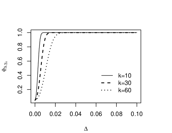
Recall that $\psi_{n}^{dis}\to 1$ as $\Delta\gg\sqrt{kp}/n$ and that $\psi_{n}^{cen}\to 1$ as $\Delta\gg\sqrt{p}/n$. Then the asymptotic relative efficiency of the distributed test statistic to the centralized one can be measured by the ratio $(\sqrt{p}/n)/(\sqrt{kp}/n)=\sqrt{1/k}$.

Although Hotelling $T^{2}$ test is a classical one, it has serious limitations when the dimension $p$ is comparable to, or larger than the sample size $n$. Obviously, the test statistic is not well defined for $p>n$ because of the singularity of the sample covariance matrix. Moreover, Hotelling $T^{2}$ test is also known to perform poorly when $p/n\to r\in(0,1)$. For example, Dempster 1958 proposed the non-exact test in high dimension. Bai and Saranadasa 1996 further found that even when Hotelling $T^{2}$ statistic is well defined, Dempster’s non-exact test is more powerful than the Hotelling $T^{2}$ for $p/n\to r\in(0,1)$.

To overcome the limitations of Hotelling $T^{2}$ test. Many test statistics are developed by replacing the inverse of sample covariance matrix in Hotelling $T^{2}$ statistic with a diagonal matrix or the identity matrix. These statistics are applicable to high-dimensional cases and to more general distributions beyond normal. For example, Bai and Saranadasa 1996 assumed the following model: $X_{i}=\Lambda W_{i}+\mbox{\boldmath{$\mu$}}_{i}$, for $i=1,\cdots,n$, where $\Lambda$ is a $p\times m$ non-random matrix for some $m\geq p$ such that $\Lambda\Lambda^{\top}=\Sigma$, and $\{W_{i}\}_{i=1}^{n}$ are $m$-dimensional vectors satisfying $E(W_{i})=0$ and ${\rm cov}(W_{i})=I_{m}$, the $m\times m$ identity matrix. And they assumed $p/n\to r>0$, that is, $p$ can be comparable to $n$ or larger than $n$. This model includes the normal distribution as a special case. Instead of using Mahalanobis distance, Bai and Saranadasa 1996 constructed the test statistic based on Euclidean distance as follows,

where $\bar{X}$ is the sample mean. Srivastava and Du 2008 noticed that the statistic $T_{BS}$ is not scale-invariant, which may reduce the power when the scales of different components of the random vector $X_{i}$ are quite different. As a remedy, they proposed the following statistic $T_{SD}=(\bar{X}-\mbox{\boldmath{$\mu$}}_{0})^{\top}D^{-1}(\bar{X}-\mbox{\boldmath{$\mu$}}_{0}),$ where $D={\rm diag}(n\hat{\sigma}_{11}/(n-1),\cdots,n\hat{\sigma}_{pp}/(n-1))$, consisting of the diagonal elements of the matrix $n\hat{\Sigma}/(n-1)$ with $\hat{\Sigma}$ denoting the sample covariance matrix. In addition, it is assumed by Srivastava and Du 2008 that $n=O(p^{\zeta})$ for some $1/2<\zeta\leq 1$ with normality assumption. Furthermore, Srivastava 2009 relaxed the normality assumption, and assumed $n=O(p^{\zeta})$, $0<\zeta\leq 1$. Chen et al. 2011 proposed another test statistic

under the setting $p/n\to r\in(0,\infty)$, stabilizing the inverse of the sample covariance matrix. As an improvement to the work of Bai and Saranadasa 1996, Chen et al. 2010 proposed a statistic by removing the quadratic terms in $(\bar{X}-\mbox{\boldmath{$\mu$}}_{0})^{\top}(\bar{X}-\mbox{\boldmath{$\mu$}}_{0})$, which relaxed the restrictions on $p$ and $n$ greatly. Wang et al. 2015 considered robust testing procedures which are powerful to distributions with heavy-tailed and to data with outlying observations. In the following subsection 3.2, as an example for illustration, we apply the divide and conquer method to the test statistic of Wang et al. 2015.

To handle heavy-tailed distributions, Wang et al. 2015 assumed that $X_{i}$’s are $i.i.d.$ variables following an elliptical distribution. Specifically,

where $\Gamma$ is a $p\times p$ matrix, $U_{i}$ is a random vector uniformly distributed on the unit sphere in $\mathbb{R}^{p}$, and $R_{i}$ is a nonnegative random variable independent of $U_{i}$. For the hypothesis testing (1.1), the centralized test statistic in Wang et al. 2015 is as follows

where $Z_{i}=(X_{i}-\mbox{\boldmath{$\mu$}}_{0})/\|X_{i}-\mbox{\boldmath{$\mu$}}_{0}\|$ if $X_{i}\neq\mbox{\boldmath{$\mu$}}_{0}$, $Z_{i}=0$ if $X_{i}=\mbox{\boldmath{$\mu$}}_{0}$, and $\|X_{i}\|$ denotes the $L_{2}$ norm of $X_{i}$. When data are stored at random in $k$ machines, $G_{cen,n}$ can be computed as follows. For $l=1,\cdots,k$, we compute local sample sum $B_{l}=\sum_{i\in S_{l}}Z_{i}$ and transmit $B_{l}$’s to the central hub. Then $G_{cen,n}=[(\sum_{l=1}^{k}B_{l})^{\top}(\sum_{l=1}^{k}B_{l})-n]/2$.

However, when $p$ is large and communication cost is prohibitively heavy, we are interested in the following distributed version of the statistic

where $G_{l}=\sum\limits_{i,j\in S_{l},j<i}Z_{i}^{\top}Z_{j}\in\mathbb{R}$ and $S_{l}$ is the indices of observations in $l$-th machine. To obtain $G_{dis,n}$, only scalars $G_{l}$’s need to be transmitted to the hub. Comparison of the powers of $G_{cen,n}$ and $G_{dis,n}$ is an interesting problem. To derive the asymptotic properties of $G_{cen,n}$ and $G_{dis,n}$, we need the following conditions, where ${\rm Tr}(\cdot)$ denotes the trace and $\Sigma=\mathrm{cov}(X_{i})$.

• (A2)

  Let $a_{m,\Sigma}=\mathrm{Tr}(\Sigma^{m})$ for any positive integer $m$, and $a_{\max}$ and $a_{\min}$ be the maximum and minimum eigenvalues of $\Sigma$, respectively. Assume that ($i$) $a_{4,\Sigma}=o(a_{2,\Sigma}^{2})$; ($ii$) $(a^{4}_{1,\Sigma}/a^{2}_{2,\Sigma})\exp\big\{-a^{2}_{1,\Sigma}/(128pa_{\max}^{2})\big\}=o(1)$; ($iii$) $a_{\max}=o(a_{1,\Sigma})$; ($iv$) $\exp\big\{-a_{1,\Sigma}^{2}/(256pa^{2}_{\max})\big\}=o\big(\min\{a_{\max}/a_{1,\Sigma},a_{\min}/a_{\max}\}).$

• (A3)

  For some $0<\delta<1$, $\|\mbox{\boldmath{$\mu$}}-\mbox{\boldmath{$\mu$}}_{0}\|^{2\delta}E\big(\|\epsilon_{i}\|^{-2-2\delta}\big)=o\big(E^{2}\big(\|\epsilon_{i}\|^{-1}\big)\big).$

• (A4)

  $\|\mbox{\boldmath{$\mu$}}-\mbox{\boldmath{$\mu$}}_{0}\|^{2}E\big(\|\epsilon_{i}\|^{-2}\big)=o\big(\min\{a_{2,\Sigma}/(na_{\max}a_{1,\Sigma}),a^{1/2}_{2,\Sigma}/(n^{1/2}a_{1,\Sigma})\}\big).$

These conditions are exactly the conditions (C1)–(C6) in Wang et al. 2015. Let

Wang et al. 2015 proved the following conclusion on the centralized test statistic $G_{cen,n}$.

To discuss the asymptotic properties of the distributed statistic $G_{dis,n}$, we assume

• (A4^′)

  $\|\mbox{\boldmath{$\mu$}}-\mbox{\boldmath{$\mu$}}_{0}\|^{2}E\big(\|\epsilon_{i}\|^{-2}\big)=o\big(\min\{ka_{2,\Sigma}/(na_{\max}a_{1,\Sigma}),(ka_{2,\Sigma})^{1/2}/(n^{1/2}a_{1,\Sigma})\}\big).$

It is seen that (A4^′) is weaker than (A4). The asymptotic distribution of $G_{dis,n}$ is as follows.

Under the condition ($i$) in (A2), when $\min\{n_{1},p\}\to\infty$ , following Chen et al. 2010 and Wang et al. 2015, ${\rm Tr}(B_{\epsilon}^{2})$ can be estimated using only the data in the first machine, specifically,

where $\bar{Z}^{*}=(n_{1}-2)^{-1}\sum_{i\in S_{1}}Z_{i}$, We compare the centralized test with the distributed one in terms of the asymptotic relative efficiency. Let $\eta_{p}=(\mbox{\boldmath{$\mu$}}-\mbox{\boldmath{$\mu$}}_{0})^{\top}A_{\epsilon}^{2}(\mbox{\boldmath{$\mu$}}-\mbox{\boldmath{$\mu$}}_{0})(1+o(1))/\sqrt{2{\rm Tr}(B_{\epsilon}^{2})}$. Theorem 3 implies that under $H_{1}$, the distributed test with sample size $n$ has the power

On the other hand, by Wang et al. 2015, the centralized statistic $G_{cen,N}$ with sample size $N$ has the power

Then we describe the asymptotic relative efficiency of the distributed test to the centralized one by the ratio of the sample sizes $N/n$ such that $\psi_{N}^{cen}=\psi_{n}^{dis}$, that is, $N/n=1/\sqrt{k}$. Thus, the distributed test is less efficient than that of the centralized one.

Combining the results in Section 2 and 3 together we derive the following conclusions. For the distributed test statistic constructed using the divide and conquer method, there is a tradeoff between the efficiency represented by the power and the communication cost. On the other hand, when point estimations are concerned, many works have shown that in terms of means square error (MSE), the estimators constructed using divide and conquer can be the same order as that of the centralized estimators (Chen and Xie 2014; Zhang et al. 2015; Jordan et al. 2019; Volgushev et al. 2019; Chen and Peng 2018, etc.).

We illustrate the performance of the distributed tests and compare them with that of the centralized ones by simulations. For any integer $m$, denote by $\mathbf{0}_{m}$ the vector of zero in $\mathbb{R}^{m}$, and $\mathbf{1}_{m}$ the vectors in $\mathbb{R}^{m}$ with elements 1. Let $\mbox{\boldmath{$\mu$}}_{0}=\mathbf{0}_{p}$, and consider the following hypothesis testing problem

For both distributed and centralized tests, we repeat 500 times to compute the type I error and the means of the power.

Example 1. We consider the case of $pk<n$. Let $\{X_{i}\}_{i=1}^{n}$ be $i.i.d.$ $p$-dimensional random vectors from the normal distribution $N_{p}(\mbox{\boldmath{$\mu$}},\Sigma)$, where $E(X_{i})=\mbox{\boldmath{$\mu$}}\in\mathbb{R}^{p}$ and $\mathrm{cov}(X_{i})=\Sigma\in\mathbb{R}^{p\times p}$. With the notation $\tilde{\Sigma}=(\tilde{\sigma}_{ij})$ with $\tilde{\sigma}_{ij}=0.5^{|i-j|}$, we assume that $\mu$ and $\Sigma$ are generated from the following four cases: (1) $\mbox{\boldmath{$\mu$}}=(c\mathbf{1}_{2}^{\top},\mathbf{0}_{p-2}^{\top})^{\top}$ and $\Sigma=I_{p}$; (2) $\mbox{\boldmath{$\mu$}}=c\mathbf{1}_{p}$ and $\Sigma=I_{p}$; (3) $\mbox{\boldmath{$\mu$}}=(c\mathbf{1}_{2}^{\top},\mathbf{0}_{p-2}^{\top})^{\top}$ and $\Sigma=\tilde{\Sigma}$; (4) $\mbox{\boldmath{$\mu$}}=c\mathbf{1}_{p}$ and $\Sigma=\tilde{\Sigma}$, where $c$ is a constant, and different values of $c$ will be considered.

We set $p=50$ and 100 respectively. For the distributed test, we set $k=30,50$, and 70, respectively, and split the data randomly into $k$ machines with equal sizes. For each setting, we estimate the sizes of the test by the frequency of rejection in 500 replicas. Simulation results on the type I error for $k=30$ are presented in Table 1, and those of $k=50$ and $k=70$ are similar and are omitted.

The simulation results with $n=10000$ and $p=50$ for different $k$ are presented in Figure 2, and results on $p=100$ are similar and are omitted. From Figure 2, it is seen that the power of distributed test increases to 1, as $c$ increases. In addition, the distributed test is less powerful than the centralized one, which coincides with the theoretical results.

Example 2. We consider the high-dimensional cases where $p>n$. Let $\{X_{i}\in\mathbb{R}^{p},1\leq i\leq n\}$ be $i.i.d.$ sample with the mean $E(X_{i})=\mbox{\boldmath{$\mu$}}$ and covariance $\Sigma=(\sigma_{ij})$. Let $p=1000$ and $n=900$. Moreover, we take $k=10,20$ and 30, and split the data randomly into $k$ machines such that each machine has samples of size $n/k$, which is much smaller than $p$. Let $\mbox{\boldmath{$\mu$}}=(c\mathbf{1}_{20}^{\top},\mathbf{0}_{p-20}^{\top})^{\top}$ with $c=0,0.25,0.35,0.45$, respectively, and $c=0$ implies that $H_{0}$ is true. $\Sigma$ is taken as either $\Sigma_{1}$ or $\Sigma_{2}$, defined as $\Sigma_{1}=(\sigma_{1,ij})$ with $\sigma_{1,ij}=0.8^{|i-j|}$, and $\Sigma_{2}=(\sigma_{2,ij})$ with $\sigma_{2,ii}=1$ and $\sigma_{2,ij}=0.2$ for $i\neq j$. We consider two cases: (1) $X_{i}$ follows the normal distribution $N_{p}(\mbox{\boldmath{$\mu$}},\Sigma)$. (2) $X_{i}$ follows the multivariate $t$ distribution $t_{\nu}(\mbox{\boldmath{$\mu$}},\Sigma)$ with the degrees of freedom $\nu=3$.

Simulation results are presented in Table 2. From Table 2, it is seen that the type I error is controlled well for both methods. In addition, we see that the powers of the distributed test statistics decrease as $k$ grows and is lower than those of the centralized ones, which coincides with the theoretical findings.

We compare the distributed and centralized tests on the Statlog (Landsat Satellite) dataset from the UCI machine learning repository (Dua and Graff 2017), a multi-spectral data having 36 covariates and 6 class labels. The covariates contain the pixel values of the four spectral bands of each of the 9 pixels in the $3\times 3$ neighbourhood in a satellite image, and the response is the classification label of the central pixel. This data have been analyzed by several authors (Tang et al. 2005; Kim and Ghahramani 2012, etc.). In multi-spectral data analysis, predictors in each class are generally viewed as normal vectors in the literature of geography and biology (Pickup et al. 1993; Bauer et al. 2011; Natsagdorj et al. 2017, etc.). For this data, classes 3 and 7 represent grey soil and very damp grey soil with the sample size being 1357 and 1508, respectively. After applying the Box-Cox transformations on variables of indices 9, 24, 35, and 36, we find that the data in each class are approximately normal. Denoting by $\mbox{\boldmath{$\mu$}}_{g}$ the mean of class $g$ with $g\in\{3,7\}$, we aim to test $H_{0}:\mbox{\boldmath{$\mu$}}_{3}-\mbox{\boldmath{$\mu$}}_{7}=0$.

We select $n=1000$ observations at random for each class, denoted as $\{X_{gi},i=1,\cdots,n,g=3,7\}$, and construct the observations $Z_{i}=X_{3i}-X_{7i},1\leq i\leq n$. The problem we considered becomes $H_{0}:E(Z_{i})=0$. We apply the centralized Hotelling $T^{2}$ test and the distributed one with $k=15$ and $25$, respectively, and compute the $p$-values. Repeating the procedure 100 times, the results of the average of the $p$-values are presented in the column associated with $\delta=0$ in Table 3.

Furthermore, to compare the powers of the centrialized test with those of the distributed one, we shift the means such that two populations are close to each other. Reminding that there are 357 and 508 observations left for classes 3 and 7, respectively, then for $g=3$ and 7, $\mbox{\boldmath{$\mu$}}_{g}$ can be estimated by the sample mean of these remaining observations in class $g$, denoted as $\bar{\mbox{\boldmath{$\mu$}}}_{g}$, which is independent of $Z_{i}$’s. Then we shift the mean $\mbox{\boldmath{$\mu$}}_{3}$ of class 3 to $\mbox{\boldmath{$\mu$}}_{3}-\delta(\bar{\mbox{\boldmath{$\mu$}}}_{3}-\bar{\mbox{\boldmath{$\mu$}}}_{7})$ with $0\leq\delta<1$, which is equivalent to shifting $Z_{i}$ to $Z_{i,\delta}=Z_{i}-\delta(\bar{\mbox{\boldmath{$\mu$}}}_{3}-\bar{\mbox{\boldmath{$\mu$}}}_{7})$. Clearly, when $\mbox{\boldmath{$\mu$}}_{3}\neq\mbox{\boldmath{$\mu$}}_{7}$, distinguishing two classes becomes more difficult for large $\delta$. We repeat the procedure for 100 times and compute the average of the $p$-values. The results are presented in Table 3. It is seen that the centralized test performs better when $\delta$ is close to 1.

Recalling that $T_{l}^{2}\sim T^{2}(p,n_{l}-1)$ and using the connection between Hotelling $T^{2}$ distribution and the $F$-distribution, we have

Then, it is easy to derive that

References

- Anderson (1984) Anderson, T. W., 1984. An introduction to multivariate statistical analysis, 3rd Edition. World Scientific Publishing Co.
- Bai and Saranadasa (1996) Bai, Z., Saranadasa, H., 1996. Effect of high dimension: by an example of a two sample problem. Statistica Sinica 6 (2), 311–329.
- Battey et al. (2018) Battey, H., Fan, J., Liu, H., Lu, J., Zhu, Z., 2018. Distributed testing and estimation under sparse high dimensional models. The Annals of Statistics 46 (3), 1352–1382.
- Bauer et al. (2011) Bauer, S. D., Korč, F., Förstner, W., 2011. The potential of automatic methods of classification to identify leaf diseases from multispectral images. Precision Agriculture 12 (3), 361–377.
- Billingsley (2008) Billingsley, P., 2008. Probability and measure. John Wiley & Sons.
- Chakraborty et al. (2017) Chakraborty, A., Chaudhuri, P., et al., 2017. Tests for high-dimensional data based on means, spatial signs and spatial ranks. The Annals of Statistics 45 (2), 771–799.
- Chen et al. (2011) Chen, L. S., Paul, D., Prentice, R. L., Wang, P., 2011. A regularized Hotelling’s test for pathway analysis in proteomic studies. Journal of the American Statistical Association 106 (496), 1345–1360.
- Chen and Peng (2018) Chen, S. X., Peng, L., 2018. Distributed statistical inference for massive data. arXiv preprint arXiv:1805.11214.
- Chen et al. (2010) Chen, S. X., Qin, Y.-L., et al., 2010. A two-sample test for high-dimensional data with applications to gene-set testing. The Annals of Statistics 38 (2), 808–835.
- Chen and Xie (2014) Chen, X., Xie, M.-g., 2014. A split-and-conquer approach for analysis of extraordinarily large data. Statistica Sinica, 1655–1684.
- Davison (1992) Davison, A., 1992. Treatment effect heterogeneity in paired data. Biometrika 79 (3), 463–474.
- Dempster (1958) Dempster, A. P., 1958. A high dimensional two sample significance test. The Annals of Mathematical Statistics, 995–1010.
- Dobriban and Sheng (2021) Dobriban, E., Sheng, Y., 2021. Distributed linear regression by averaging. The Annals of Statistics 49 (2), 918–943.
- Dong et al. (2016) Dong, K., Pang, H., Tong, T., Genton, M. G., 2016. Shrinkage-based diagonal Hotelling’s tests for high-dimensional small sample size data. Journal of Multivariate Analysis 143, 127–142.
- Dua and Graff (2017)
Dua, D., Graff, C., 2017. UCI machine learning repository.
URL http://archive.ics.uci.edu/ml - Edward Jackson (1985) Edward Jackson, J., 1985. Multivariate quality control. Communications in Statistics-Theory and Methods 14 (11), 2657–2688.
- Fan et al. (2019) Fan, J., Wang, D., Wang, K., Zhu, Z., 2019. Distributed estimation of principal eigenspaces. The Annals of Statistics 47 (6), 3009–3031.
- Guo et al. (2019) Guo, Z.-C., Lin, S.-B., Shi, L., 2019. Distributed learning with multi-penalty regularization. Applied and Computational Harmonic Analysis 46 (3), 478–499.
- Haug et al. (2011) Haug, L. S., Huber, S., Schlabach, M., Becher, G., Thomsen, C., 2011. Investigation on per-and polyfluorinated compounds in paired samples of house dust and indoor air from Norwegian homes. Environmental Science & Technology 45 (19), 7991–7998.
- Hsieh et al. (2014) Hsieh, C.-J., Si, S., Dhillon, I. S., 2014. A divide-and-conquer solver for kernel support vector machines. In: International Conference on Machine Learning. pp. 566–574.
- Jordan et al. (2019) Jordan, M. I., Lee, J. D., Yang, Y., 2019. Communication-efficient distributed statistical inference. Journal of the American Statistical Association 114 (526), 668–681.
- Kim and Ghahramani (2012) Kim, H.-C., Ghahramani, Z., 2012. Bayesian classifier combination. In: Artificial Intelligence and Statistics. PMLR, pp. 619–627.
- Lee et al. (2012) Lee, S. H., Lim, J., Li, E., Vannucci, M., Petkova, E., 2012. Order test for high-dimensional two-sample means. Journal of Statistical Planning and Inference 142 (9), 2719–2725.
- Li et al. (2020) Li, H., Aue, A., Paul, D., Peng, J., Wang, P., et al., 2020. An adaptable generalization of Hotelling’s test in high dimension. The Annals of Statistics 48 (3), 1815–1847.
- Li and Zhao (2020) Li, M., Zhao, J., 2020. Communication-efficient distributed linear discriminant analysis for binary classification. Statistica Sinica.
- Lin et al. (2017) Lin, S.-B., Guo, X., Zhou, D.-X., 2017. Distributed learning with regularized least squares. Journal of Machine Learning Research 18 (1), 3202–3232.
- Natsagdorj et al. (2017) Natsagdorj, E., Renchin, T., Kappas, M., Tseveen, B., Dari, C., Tsend, O., Duger, U.-O., 2017. An integrated methodology for soil moisture analysis using multispectral data in mongolia. Geo-spatial Information Science 20 (1), 46–55.
- Patnaik (1949) Patnaik, P. B., 1949. The non-central - and -distributions and their applications. Biometrika (1-2), 1–2.
- Pickup et al. (1993) Pickup, G., Chewings, V., Nelson, D., 1993. Estimating changes in vegetation cover over time in arid rangelands using Landsat MSS data. Remote sensing of Environment 43 (3), 243–263.
- Rubin (2006) Rubin, D. B., 2006. Matched sampling for causal effects. Cambridge University Press.
- Srivastava (2009) Srivastava, M. S., 2009. A test for the mean vector with fewer observations than the dimension under non-normality. Journal of Multivariate Analysis 100 (3), 518–532.
- Srivastava and Du (2008) Srivastava, M. S., Du, M., 2008. A test for the mean vector with fewer observations than the dimension. Journal of Multivariate Analysis 99 (3), 386–402.
- Srivastava et al. (2016) Srivastava, R., Li, P., Ruppert, D., 2016. RAPTT: An exact two-sample test in high dimensions using random projections. Journal of Computational and Graphical Statistics 25 (3), 954–970.
- Szabó and Van Zanten (2019) Szabó, B., Van Zanten, H., 2019. An asymptotic analysis of distributed nonparametric methods. Journal of Machine Learning Research 20 (87), 1–30.
- Tang et al. (2005) Tang, E. K., Suganthan, P. N., Yao, X., Qin, A. K., 2005. Linear dimensionality reduction using relevance weighted LDA. Pattern Recognition 38 (4), 485–493.
- Tian and Gu (2017) Tian, L., Gu, Q., 2017. Communication-efficient distributed sparse linear discriminant analysis. In: Artificial Intelligence and Statistics. PMLR, pp. 1178–1187.
- Volgushev et al. (2019) Volgushev, S., Chao, S.-K., Cheng, G., et al., 2019. Distributed inference for quantile regression processes. The Annals of Statistics 47 (3), 1634–1662.
- Wang et al. (2015) Wang, L., Peng, B., Li, R., 2015. A high-dimensional nonparametric multivariate test for mean vector. Journal of the American Statistical Association 110 (512), 1658–1669.
- Xu et al. (2016) Xu, G., Lin, L., Wei, P., Pan, W., 2016. An adaptive two-sample test for high-dimensional means. Biometrika 103 (3), 609–624.
- Ye et al. (2002) Ye, N., Emran, S. M., Chen, Q., Vilbert, S., 2002. Multivariate statistical analysis of audit trails for host-based intrusion detection. IEEE Transactions on Computers 51 (7), 810–820.
- Zhang et al. (2015) Zhang, Y., Duchi, J., Wainwright, M., 2015. Divide and conquer kernel ridge regression: A distributed algorithm with minimax optimal rates. Journal of Machine Learning Research 16 (1), 3299–3340.
- Zhang et al. (2013) Zhang, Y., Duchi, J. C., Wainwright, M. J., 2013. Communication-efficient algorithms for statistical optimization. The Journal of Machine Learning Research 14 (1), 3321–3363.