Transformations of 2-port networks and tiling by rectangles

Svetlana Shirokovskikh

Abstract

In this paper, we study 2-port networks and introduce new concepts of voltage drop and $\Pi$ -equivalence. The main result is that each planar network is $\Pi$ -equivalent to a network with no more than 5 edges. This implies that if an octagon in the shape of the letter $\Pi$ can be tiled by squares then it can be tiled by no more than 5 rectangles with rational aspect ratios. Kenyon’s theorem from 1998 proves this only for 6 rectangles.

1 Introduction

We study 2-port networks, that is, weighted graphs with four marked vertices decomposed into two pairs called ports. A visual example of such a network is a computer with two USB-ports or a flashlight with two batteries. In two-port circuits, instead of the voltages of marked vertices, we specify the differences of voltages for each port. At the same time, we require that if some current flows into one vertex of a port, then the same current flows out of the second vertex (Figure 1; we give precise definitions in Section 2.2).

Refer to caption — Figure 1: A two-port network (see Section 2.2).

We introduce a new (albeit natural) concept of voltage drop between ports and a new $\Pi$ -equivalence relation that requires not only the same incoming currents in two networks, but also the same voltage drop between ports.

These concepts are interesting from the engineering point of view. If we perform network transformations and keep the incoming currents only, without preserving the voltage drop, then the voltage difference between the vertices from different ports can become large. Informally, a short circuit may occur, disrupting the normal operation of the network. For example, a computer can burn out if you re-solder it, keeping only voltages and currents through the USB-ports, but not the voltage drop. $\Pi$ -equivalent transformations avoid such problems.

The main result of this work is that each planar network is $\Pi$ -equivalent to a network with no more than 5 edges (Theorem 3.7), and the number 5 is minimal (Example 3.12). Interestingly, if we require preservation of just incoming currents without preservation of the voltage drop, then we can end up with only 3 edges (Remark 3.9).

The proof uses $\Pi$ -equivalent transformations to reduce the number of edges in the network. The simplest of these transformations are well known; they are shown in Figure 2 (see [5, 7, 10]). We introduce a new Box-H transformation (Figure 3.6).

New results on voltage drop and $\Pi$ -equivalence make it possible to solve new tiling problems (thanks to the well-known physical interpretation of tilings by R. L. Brooks, K. A. B. Smith, A. G. Stone and W. T. Tutte [4], described in detail in [8]). They imply that if an octagon in the shape of the letter $\Pi$ can be tiled by squares then it can be tiled by no more than 5 rectangles with rational aspect ratios (Theorem 1.4). The known Kenyon theorem (Theorem 2.8) proves this only for $6$ rectangles.

1.1 Transformations of two-port networks

Transformations of two-port networks that keep incoming currents have been studied in the literature [1, 2, 3]. We will give some examples.

For instance, it is easy to see that for the same differences of incoming voltages the two-port networks in Figure 4 have the same incoming currents. Indeed, if in the network to the right we swap the vertices in each port ( $\{1,4\}$ and $\{2,3\}$ ), then we get the network to the left, but differences of incoming voltages change their sign. Therefore, the current flowing out of vertex 1 of the left network is equal to the current flowing into vertex 4 of the right network. In two-port networks, we require that if some current flows into one vertex of a port, then the same flows out of the second vertex. Therefore, in the left network, the current flowing out vertex 1 is equal to the current flowing into vertex 4. By transitivity, the current flowing into vertex 4 is the same in the left and right networks. For the other vertices, the proof is similar.

We say that a two-port network with ports $\{1,4\}$ and $\{2,3\}$ is symmetric, if there exists an automorphism of a weighted graph which swap vertices in each pair $\{1,2\}$ and $\{3,4\}$ .

In 1927 Barlett [2] proved that for any symmetric two-port network there exists a two-port network with four edges ${12},{34},{13},$ and ${24}$ with the same incoming currents (Figure 5).

1.2 Tilings

In this section, we give a short overview of known results on tilings by squares.

A natural question is: which polygons can be tiled by squares? The answer for rectangles was obtained by Max Dehn in 1903.

Theorem 1.1 (Dehn, 1903).

[6] A rectangle can be tiled by squares (not necessarily equal) if and only if the ratio of two orthogonal sides of the rectangle is rational.

In this paper, we consider only tilings by finitely many arbitrary squares.

In the case of hexagons the answer was obtained by R. Kenyon almost a hundred years later.

Theorem 1.2 (Kenyon, 1998).

(Cf. [7, Theorem 9]) Let $A_{1}A_{2}A_{3}A_{4}A_{5}A_{6}$ be a hexagon with right angles whose vertices are enumerated counterclockwise starting from the vertex of the nonconvex angle. The hexagon $A_{1}A_{2}A_{3}A_{4}A_{5}A_{6}$ can be tiled by squares if and only if the system

\begin{cases}A_{3}A_{4}\cdot x+A_{1}A_{2}\cdot y=A_{2}A_{3},\\ A_{5}A_{6}\cdot z-A_{1}A_{2}\cdot y=A_{6}A_{1};\end{cases}

(1)

has a nonnegative rational solution $x,y,z$ .

Figure 6: [8] The hexagon

A_{1}A_{2}A_{3}A_{4}A_{5}A_{6}

Figure 6 explains why if system (1) has a rational solution $x,y,z\geqslant 0$ then one can dissect the hexagon into $3$ rectangles of aspect ratios $x,y,z$ and then into squares.

A polygon is called orthogonal if its sides are parallel to the coordinate axes.

We say that a polygon is generic, if the $x$ -coordinates of the sides parallel to the $y$ -axis are pairwise distinct.

Theorem 1.3.

(Corollary from Theorem 2.8 and Lemma 2.12 below; Kenyon, 1998) Let P be a generic orthogonal polygon with 2n sides. If it can be tiled by squares then it can be tiled by not more than $n(n-1)/2$ rectangles with rational aspect ratios. In particular, a generic orthogonal hexagon and octagon can be tiled by not more than 3 and 6 rectangles with rational side ratios, respectively.

In this paper we give a proof of the following stronger assertion on a $\Pi$ -shaped octagon.

Let $ABCD$ and $A^{\prime}B^{\prime}C^{\prime}D^{\prime}$ be rectangles such that $A$ and $D$ lie on $A^{\prime}D^{\prime}$ whereas $B$ and $C$ lie strictly inside $A^{\prime}B^{\prime}C^{\prime}D^{\prime}$ . Then the closure of the complement $A^{\prime}B^{\prime}C^{\prime}D^{\prime}\setminus ABCD$ is called a $\Pi$ -shaped octagon (Figure 7).

Theorem 1.4.

If a $\Pi$ -shaped octagon can be tiled by squares, then it can be tiled by no more than 5 rectangles with rational aspect ratios.

1.3 Organization of the paper

In Section 2, we recall known definitions and theorems on electrical networks. In Subsection 2.1, we give rigorous definitions of an electrical network, its response, and equivalence. In addition, we introduce some equivalent transformations. In Subsection 2.2, we give a definition of a two-port network and generalize the concept of response to this set up. In short Subsection 2.3, we give a lemma that connects tilings and electrical networks.

In Section 3, we introduce the new concepts of voltage drop and $\Pi$ -equivalence. Then we prove the $\Pi$ -equivalence of a Box-network and an H-network (Figure 3.6). Then we state and prove the main theorem of this paper (Theorem 3.7). After that, we give an example showing that the assumptions of the theorem are sharp.

In Section 4, using Theorem 3.7, we prove Theorem 1.4 on tilings of a $\Pi$ -shaped octagon. Finally, we give an example of an octagon which cannot be tiled by less than 5 rectangles with rational aspect ratios.

2 Preliminaries

2.1 Electrical networks

An electrical network with ${t}$ terminals is a connected graph with a nonnegative real number (conductance) assigned to each edge, and ${t}$ marked (boundary) vertices. For simplicity we assume that the graph has neither multiple edges nor loops. Generalizations for graphs with multiple edges are left to the reader.

We say that an electrical network is planar, if the graph is embedded in the unit disc in such a way that the boundary vertices belong to the boundary of the disc and the edges have no common points except their common vertices.

Fix an enumeration of the vertices ${1}$ , ${2}$ , ${\dots}$ , ${n}$ such that ${1,\dots,t}$ are the boundary ones. If an electrical network is planar then we assume that the boundary vertices are enumerated counterclockwise along the boundary of the unit disc. Denote by ${kl}$ the edge between the vertices ${k}$ and ${l}$ . Denote by $c_{kl}$ the conductance of the edge ${kl}$ . Set $c_{kl}=0$ , if there is no edge between ${k}$ and ${l}$ .

An electrical circuit is an electrical network along with ${t}$ real numbers ${U_{1},\dots,U_{t}}$ (incoming voltages) assigned to the boundary vertices.

Each electrical circuit gives rise to certain numbers $U_{k}$ , where $1\leqslant k\leqslant n$ (voltages at the vertices), and $I_{kl}$ , where $1\leqslant k,l\leqslant n$ (currents through the edges, where ${I_{kl}}=0$ if there is no edge $kl$ according to axiom (C) below). These numbers are defined by the following $2$ axioms:

(C)

The Ohm law. For each pair of vertices $k,l$ we have $I_{kl}=c_{kl}(U_{k}-U_{l})$ .
(I)

The Kirchhoff current law. For each vertex $k>t$ we have $\sum_{l=1}^{n}I_{kl}=0$ .

The numbers $U_{k}$ and $I_{kl}$ are well-defined by these axioms by the following classical result.

Theorem 2.1.

[8, Theorem 2.1.] For any electrical circuit the system of linear equations (C), (I) in variables $U_{k}$ , where $t<k\leqslant n$ , and $I_{kl}$ , where $1\leqslant k,l\leqslant n$ , has a unique solution.

The reciprocal of the conductance is called the resistance. Denote by $R_{kl}$ the resistance of the edge ${kl}$ . Numbers $(I_{1},\dots,I_{t}):=({{\sum_{k=1}^{n}I_{1k}}},\dots,{{\sum_{k=1}^{n}I_{tk}}})$ are called incoming currents. The linear map $\mathds{R}^{t}\to\mathds{R}^{t}$ : $({U_{1}},\dots,{U_{t}})\mapsto(I_{1},\dots,I_{t})$ is called the response of the network. The description of the responses of planar networks is very interesting (see [5], [7]). Two networks are called equivalent if their responses are equal.

The results of this section are well-known and easily deduced from the definitions (see [9, Theorem on electric transformations in §2.3]).

Proposition 2.2.

(Figure 8) Let $xy$ be an edge such that $U_{x}=U_{y}$ for any incoming voltages. For each $z\neq x$ replace each edge $zy$ in the network by an edge $zx$ of the same resistance and then remove the edge $xy$ and the vertex $y$ . Then we get an equivalent network.

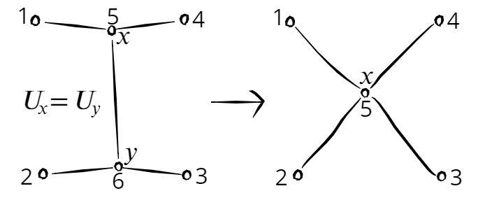
This transformation is called combining the vertices $x$ and $y$ with the same voltages.

Remark 2.3.

(Parallel connection, Figure 2, top right). If a network has two multiple edges of resistances $a$ and $b$ , then we can replace them by one edge of resistance $ab/(a+b)$ between the same vertices. The resulting network is equivalent to the initial one. Using such parallel connections, we can always transform any network with multiple edges into an equivalent network without multiple edges. The latter network has less edges than the former one. If the resistances of edges in the original network are rational, then the resistances in the new network are also rational. This allows us to consider only networks without multiple edges in what follows.

Proposition 2.4.

(Figure 2, top left) For each $a,b>0$ , the following two networks with two terminals are equivalent:

(1)

The network with three vertices and two edges 13 and 23 of resistances

$\displaystyle R_{13}=a,R_{23}=b.$
(2)

The network with two vertices and one edge 12 of resistance

$\displaystyle R_{12}=a+b.$

Corollary 2.5.

(Figure 2, top left) Let $xy$ and $yz$ be edges such that $y$ is a non-boundary vertex of degree two. Replace those two edges by an edge $xz$ of resistance $R_{xz}:=R_{xy}+R_{yz}$ and then remove the vertex $y$ . Then we get an equivalent network.

This transformation is called the series connection applied to the edges $xy$ and $yz$ .

Proposition 2.6.

(Figure 2, bottom) For each $a,b,c>0$ , the following two networks with three terminals are equivalent:

( $\Delta$ )

The network with three vertices and three edges 12, 23, 13 of resistances

$\displaystyle R_{12}=a,R_{23}=b,R_{13}=c.$
( $Y$ )

The network with four vertices and three edges 14, 24, 34 of resistances

$\displaystyle R_{14}=ac/(a+b+c),R_{24}=ab/(a+b+c),R_{34}=bc/(a+b+c).$

Corollary 2.7.

(Figure 2, bottom) Let x, y, and z be vertices such that each pair of these vertices is joined by an edge. Add a new non-boundary vertex $w$ and replace edges $xy$ , $xz$ , $yz$ by edges $xw,yw,zw$ of resistances

		$\displaystyle R_{xw}:=R_{xy}R_{xz}/(R_{xy}+R_{xz}+R_{yz}),$
		$\displaystyle R_{yw}:=R_{xy}R_{yz}/(R_{xy}+R_{xz}+R_{yz}),$
		$\displaystyle R_{zw}:=R_{xz}R_{yz}/(R_{xy}+R_{xz}+R_{yz}).$

Then we get an equivalent network.

This transformation is called the $\Delta-Y$ transformation applied to the edges $xy,yz,xz$ . The inverse transformation is called the $Y-\Delta$ transformation.

Parallel connection, series connection, $\Delta-Y$ transformation, and $Y-\Delta$ transformation are called elementary transformations (Figure. 2).

Theorem 2.8.

(Kenyon, 1998) [7, Theorem 8] For any planar network $G$ with $t$ terminals, there exists an equivalent planar network which has no more than $t(t-1)/2$ edges and is obtained from the network $G$ by a sequence of elementary transformations.

2.2 Two-port networks

A two-port network is an electrical network with 4 terminals decomposed into 2 pairs called ports.

Fix an enumeration of the vertices ${1}$ , ${2}$ , ${\dots}$ , ${n}$ such that ${1}$ , ${2}$ , ${3}$ , ${4}$ are the boundary ones decomposed into the pairs $\{1,4\}$ and $\{2,3\}$ . As before, denote by $c_{kl}$ the conductance of the edge ${kl}$ . Set $c_{kl}=0$ , if there is no edge between ${k}$ and ${l}$ . A planar two-port network is defined similarly to a planar electrical network. If a two-port network is planar then we assume that the boundary vertices are enumerated counterclockwise along the boundary of the unit disc.

A two-port circuit is a two-port network along with ${2}$ real numbers $\Delta{U_{14}}$ and $\Delta{U_{23}}$ (differences of incoming voltages), assigned to the pairs of boundary vertices.

Each two-port circuit gives rise to certain numbers $U_{k}$ , where $1\leqslant k\leqslant n$ (voltages at the vertices), and $I_{kl}$ , where $1\leqslant k,l\leqslant n$ (currents through the edges, where ${I_{kl}}=0$ if there is no edge $kl$ ). These numbers are defined by the following $4$ axioms:

(C)

The Ohm law. For each pair of vertices $k,l$ we have $I_{kl}=c_{kl}(U_{k}-U_{l})$ .
(I)

The Kirchhoff current law. For each vertex $k>4$ we have $\sum_{l=1}^{n}I_{kl}=0$ .
(P)

Port-isolation condition. ${{\sum_{l=1}^{n}I_{1l}+\sum_{l=1}^{n}I_{4l}=0}}$ .
(B)

Boundary conditions. $U_{1}-U_{4}=\Delta{U_{14}}$ and $U_{2}-U_{3}=\Delta{U_{23}}$ .

Theorem 2.9.

For any two-port electrical circuit there exist a unique collection ${I_{kl}}$ , ${1\leqslant k,l\leqslant n}$ , and a unique up to adding a constant collection ${U_{k}}$ , ${1\leqslant k\leqslant n}$ , that satisfy conditions (C), (I), (P), (B).

The proof of Theorem 2.9 is well-known, but we present it for completeness. It is obtained similarly to the proof of Theorem 2.1 from [8] and uses the following lemma.

Lemma 2.10.

[8, Lemma 5.1] Consider an electrical network with the vertices ${1,\dots,n}$ such that ${1,\dots,t}$ are the boundary ones. Suppose that the numbers ${U_{k}}$ , where ${1\leqslant k\leqslant n}$ , and ${I_{kl}}$ , where ${1\leqslant k,l\leqslant n}$ , satisfy the Ohm law (C) and the Kirchhoff current law (I) from §2. Set ${I_{u}=\sum_{k=1}^{n}I_{uk}}$ . Then

\sum\limits_{1\leqslant k<l\leqslant n}(U_{k}-U_{l})I_{kl}=\sum\limits_{1\leqslant u\leqslant t}U_{u}I_{u}.

Proof of Theorem 2.9.

Take $C\in\mathds{R}$ . It is easy to see that a collection of currents ${I_{kl}}$ and a collection of voltages ${U_{k}}$ satisfies properties (C), (I), (P), (B) if and only if the collection of currents ${I_{kl}}$ and the collection of voltages ${U_{k}}+C$ satisfies the same properties. We prove the existence and uniqueness of solution under the additional condition $U_{1}=0$ .

Uniqueness. Suppose there are two collections of currents ${I^{I,II}_{kl}}$ and voltages ${U^{I,II}_{k}}$ satisfying laws (C), (I), (P), (B) and ${U^{I}_{1}=U^{II}_{2}=0}$ for some differences of incoming voltages $\Delta{U_{14}}^{I}$ = $\Delta{U_{14}}^{II}$ and $\Delta{U_{23}}^{I}$ = $\Delta{U_{23}}^{II}$ . Then their differences ${I_{kl}=I^{I}_{kl}-I^{II}_{kl}}$ and ${U_{k}=U^{I}_{k}-U^{II}_{k}}$ satisfy laws (C), (I), (P), (B) for zero incoming voltages $\Delta{U_{14}}=0$ and $\Delta{U_{23}}=0$ . Then $U_{1}=U_{4}$ and $U_{2}=U_{3}$ . Using $(I)$ and $(P)$ , we obtain $I_{1}=-I_{4}$ and $I_{2}=-I_{3}$ . It follows that $\sum_{u=1}^{4}U_{u}I_{u}=0$ .

Then by Lemma 2.10 we have

\sum\limits_{1\leqslant k<l\leqslant n}(U_{k}-U_{l})^{2}c_{kl}=\sum\limits_{1\leqslant k<l\leqslant n}(U_{k}-U_{l})I_{kl}=\sum\limits_{1\leqslant u\leqslant 4}U_{u}I_{u}=0.

For each ${k,l}$ we have either ${c_{kl}>0}$ or ${c_{kl}=0}$ . Thus each summand $c_{kl}(U_{k}-U_{l})^{2}=0$ . Since the network is connected it follows that all the voltages ${U_{k}}$ are equal to each other. But $U_{1}=U_{1}^{I}-U_{1}^{II}=0$ . Hence ${U_{k}=0}$ , ${I_{kl}=0}$ , and thus ${I^{I}_{kl}=I^{II}_{kl}}$ , ${U^{I}_{k}=U^{II}_{k}}$ for each ${k,l}$ .

Existence. The number of equations in the system (C), (I), (P), (B) equals the number of variables (if we fix $U_{1}=0$ ). We have proved that the system has a unique solution for $\Delta{U_{14}}=0$ , $\Delta{U_{23}}=0$ . By the finite-dimensional Fredholm alternative it has a solution for each $\Delta{U_{14}}$ , $\Delta{U_{23}}$ . ∎

The numbers $(I_{1},I_{2}):=({{\sum_{k=1}^{n}I_{1k}}},{{\sum_{k=1}^{n}I_{2k}}})$ are called the incoming currents. The linear map $\mathds{R}^{2}\to\mathds{R}^{2}$ : $(\Delta{U_{14}},\Delta{U_{23}})\mapsto(I_{1},I_{2})$ is called the response of the two-port network.

Example 2.11.

The two-port network with four vertices and four edges $12,23,34,14$ of resistances $R_{12}=a,R_{14}=b,R_{34}=c,R_{23}=d$ (Box-network, see Figure 3.6 to the left) has the following response matrix:

${\left(\begin{matrix}(a+b+c)/(ab+ac)&-1/(a+c)\\ -1/(a+c)&(a+c+d)/(ad+cd)\end{matrix}\right)}$ .

Proof.

Using $(C),(I),(P),(B),$ we obtain the system of equations:

\begin{cases}U_{1}-U_{4}=\Delta U_{14},\\ U_{2}-U_{3}=\Delta U_{23},\\ I_{14}b=U_{1}-U_{4},\\ I_{12}a=U_{1}-U_{2},\\ I_{43}c=U_{4}-U_{3},\\ I_{23}d=U_{2}-U_{3},\\ I_{12}+I_{14}+I_{23}+I_{43}=0.\end{cases}

(2)

From this system we have:

		$\displaystyle I_{14}=\Delta{U_{14}}/b,$
		$\displaystyle I_{12}=(\Delta{U_{14}}-\Delta{U_{23}})/(a+c),$
		$\displaystyle I_{43}=(\Delta{U_{23}}-\Delta{U_{14}})/(a+c),$
		$\displaystyle I_{23}=\Delta{U_{23}}/d,$
		$\displaystyle I_{1}=I_{14}+I_{12}=((a+b+c)\Delta{U_{14}}-b\Delta{U_{23}})/(b(a+c)),$
		$\displaystyle I_{2}=I_{21}+I_{23}=((a+c+d)\Delta{U_{23}}-d\Delta{U_{14}})/(d(a+c)).$

Hence

${\left(\begin{matrix}(a+b+c)/(ab+ac)&-1/(a+c)\\ -1/(a+c)&(a+c+d)/(ad+cd)\end{matrix}\right)}\cdot{\left(\begin{matrix}\Delta{U_{14}}\\ \Delta{U_{23}}\end{matrix}\right)}={\left(\begin{matrix}{I_{1}}\\ {I_{2}}\end{matrix}\right)}$ .

∎

2.3 Electrical networks and tilings

Hereafter $P$ is an orthogonal polygon (Figure 9), i.e., a polygon with the sides parallel to the coordinate axes. Hereafter $P$ is simple, i.e., the boundary $\partial P$ is connected. Enumerate the sides of the polygon parallel to the $y$ axis counterclockwise along $\partial P$ . Denote by $t$ the number of these sides. Let $I_{u}$ be the signed length of the side $u$ , where the sign of $I_{u}$ is “ $+$ ” (respectively, “ $-$ ”) if the $P$ locally lies to the right (respectively, left) of the side $u$ . Let $U_{u}$ be the $x$ -coordinate of the side $u$ . Assume that $P$ is generic in the sense that the numbers ${U_{1},\dots,U_{t}}$ are pairwise distinct.

We say that an edge $kl$ of a circuit is essential, if $I_{kl}\neq 0$ .

Lemma 2.12.

[8, Lemma 5.4.] Let $P$ be a generic simple orthogonal polygon with $t$ vertical sides of signed lengths ${I_{1},\dots,I_{t}}$ and ${x\mbox{-co}}$ ordinates ${U_{1},\dots,U_{t}}$ . Then the following 2 conditions are equivalent:

(1)

the polygon $P$ can be tiled by $m$ rectangles with ratios of the horizontal side to the vertical equal to $R_{1},\dots,R_{m}$ ;
(2)

there is a planar electrical circuit with $t$ boundary vertices, $m$ essential edges of resistances ${R_{1},\dots,R_{m}}$ , incoming voltages ${U_{1},\dots,U_{t}}$ , and incoming currents ${I_{1},\dots,I_{t}}$ .

3 $\Pi$ -equivalence of two-port networks

Now we introduce a new concept, which appears in the paper for the first time.

The linear map $\mathds{R}^{2}\to\mathds{R}$ : $(\Delta{U_{14}},\Delta{U_{23}})\mapsto U_{1}-U_{2}$ is called the voltage drop of a two-port network. We say that two-port networks are $\Pi$ -equivalent if their responses and voltage drops are equal. In Lemma 4.1 we are going to see how these concepts naturally arise in the study of tilings by rectangles.

Example 3.1.

The Box-network (see Example 2.11 and Figure 3.6) has the voltage drop $U_{1}-U_{2}=(\Delta{U_{14}}-\Delta{U_{23}})a/(a+c)$ .

Proof.

This follows directly from (2). ∎

We note the following two obvious propositions.

Proposition 3.2.

(Figure 8, cf. Proposition 2.2) Let $xy$ be an edge of a two-port network such that $U_{x}=U_{y}$ for any differences of incoming voltages. For each $z\neq x$ replace each edge $zy$ in the network by an edge $zx$ of the same resistance and then remove the edge $xy$ and the vertex $y$ . Then we get an $\Pi$ -equivalent network.

This transformation, which generalizes the combining of vertices with the same voltages, is still called combining the vertices $x$ and $y$ with the same voltages.

Proposition 3.3.

If two electrical networks with four terminals are equivalent, then the two-port networks with the same edges and the same resistances are $\Pi$ -equivalent. In particular, elementary transformations preserve the $\Pi$ -equivalence classes of two-port networks.

Our main tool is a new transformation of two-port networks that preserves both the response and the voltage drop (Figure 3.6). This transformation in particular shows that the reciprocal of Proposition 3.3 is not true (one can check directly by computing the response matrices that it is not an equivalent transformation). A network with six vertices and five edges ${15},{25},{46},{36},{56}$ is called an H-network.

Theorem 3.4.

(Figure 3.6) For each $a,b,c,d>0$ the following two-port networks are equivalent:

(Box)

The network with four vertices and four edges $12,23,34,14$ of resistances

$\displaystyle R_{12}=a,R_{14}=b,R_{34}=c,R_{23}=d.$

(H)

The network with six vertices and five edges $15,25,36,46,56$ of resistances

		$\displaystyle R_{15}=ab/(a+b+c+d),R_{25}=ad/(a+b+c+d),R_{46}=bc/(a+b+c+d),$
		$\displaystyle R_{36}=cd/(a+b+c+d),R_{56}=bd/(a+b+c+d).$

Proof.

From Examples 2.11 and 3.1 we know the response and the voltage drop for the Box-network. Using $(C),(I),(P),(B),$ we obtain the system of equations for the H-network:

\begin{cases}U_{1}-U_{4}=\Delta U_{14},\\ U_{2}-U_{3}=\Delta U_{23},\\ I_{15}ab/(a+b+c+d)=U_{1}-U_{5},\\ I_{46}bc/(a+b+c+d)=U_{4}-U_{6},\\ I_{56}bd/(a+b+c+d)=U_{5}-U_{6},\\ I_{25}ad/(a+b+c+d)=U_{2}-U_{5},\\ I_{36}cd/(a+b+c+d)=U_{3}-U_{6},\\ I_{15}+I_{46}=0,\\ I_{15}+I_{25}-I_{56}=0,\\ I_{46}+I_{56}+I_{36}=0.\end{cases}

Using system of equations, we get

		$\displaystyle I_{15}=I_{64}=((a+b+c)\Delta{U_{14}}-b\Delta{U_{23}})/(b(a+c)),$
		$\displaystyle I_{25}=I_{63}=((a+c+d)\Delta{U_{23}}-d\Delta{U_{14}})/(d(a+c)),$
		$\displaystyle U_{1}-U_{2}=(\Delta{U_{14}}-\Delta{U_{23}})a/(a+c).$

The voltage drops and responses of the networks are the same, thus the networks are $\Pi$ -equivalent. ∎

The following corollaries are obtained similarly to [9, Proof of Theorem on electrical transformations, page 35].

Corollary 3.5.

(Figure 10) Let $xy,yz,zt,tx$ be edges of a two-port network such that $I_{xy}+I_{tz}=0$ for any differences of incoming voltages. Add 2 new non-boundary vertices $v$ and $w$ and replace edges $xy,yz,zt,tx$ by edges $xv,yv,tw,zw,vw$ of resistances

		$\displaystyle R_{xv}=R_{xy}R_{xt}/(R_{xy}+R_{xt}+R_{tz}+R_{yz}),$		(3)
		$\displaystyle R_{yv}=R_{xy}R_{yz}/(R_{xy}+R_{xt}+R_{tz}+R_{yz}),$
		$\displaystyle R_{tw}=R_{xt}R_{tz}/(R_{xy}+R_{xt}+R_{tz}+R_{yz}),$
		$\displaystyle R_{zw}=R_{tz}R_{yz}/(R_{xy}+R_{xt}+R_{tz}+R_{yz}),$
		$\displaystyle R_{vw}=R_{xt}R_{yz}/(R_{xy}+R_{xt}+R_{tz}+R_{yz}).$

Then we get a $\Pi$ -equivalent network.

Corollary 3.6.

(See the first transformation in Figure 10) Let $xy,yz,zt,tx$ be edges of a two-port network such that if we remove $xy,yz,zt,tx$ then any two vertices, where the first one is from the set $\{1,4,x,t\}$ and the second one from the set $\{2,3,y,z\}$ , are in the different connected components. Add 2 new non-boundary vertices $v$ and $w$ and replace edges $xy,yz,zt,tx$ by edges $xv,yv,tw,zw,vw$ of resistances given by formula (3). Then we get a $\Pi$ -equivalent network.

This transformation is called the Box-H transformation applied to the edges $xy,yz,zt,tx$ .

Theorem 3.7.

For each planar two-port network $G$ , there exists a $\Pi$ -equivalent planar two-port network $G^{\prime}$ satisfying the following two conditions:

(1)

The network $G^{\prime}$ has no more than 4 edges or it is the H-network.
(2)

The network $G^{\prime}$ can be obtained from the network G by elementary transformations (Figure 2), combining vertices with the same voltages (Figure 8 and Proposition 3.2), and Box-H transformations (Figure 3.6).

Remark 3.8.

If all the edges of the network $G$ have rational resistances, then the resistances of the edges of the network $G^{\prime}$ are also rational.

If we require preservation of just network response without preservation of the voltage drop, then we can end up with only 3 edges:

Remark 3.9.

For each planar two-port network, there exists a planar two-port network with the same response which has no more than 3 edges. (One can prove this using Theorem 3.7 and equality of the responses of the networks in Figure 4.)

Proof of Theorem 3.7.

Consider all planar two-port networks with the minimal number of edges that can be obtained from the network $G$ by a sequence of transformations from Theorem 3.7. Among such networks, choose the network with the maximal number of vertices. Then the obtained minimal network has no cycles of length 3, otherwise the number of vertices can be increased using the $\Delta-Y$ transformation. In addition, there are no non-boundary vertices of degree two, otherwise we can reduce the number of edges by a series connection.

By Theorem 2.8 and Proposition 3.3, this network has no more than 6 edges. If it has no more than 4 edges, then the theorem is proved. Otherwise, this network has 5 or 6 edges. Consider those two cases separately.

Case 1: the network has 5 edges. This network is either a tree or it contains cycles of length more than three.

Subcase 1: the network has no cycles. Then the network has 6 vertices. The vertices 5 and 6 are non-boundary vertices of degree no less than 3. There are 5 edges in total, hence there is the edge 56. Then this is either an H-network or I-network (a network with 6 vertices and 5 edges ${15},{45},{26},{36},{56},$ see Figure 8). If this is an I-network, then, by the Port isolation (condition (P) in §2.2) we have $I_{15}=I_{54}$ , and hence, by the Kirchhoff current law (condition (I)) we get $I_{56}=0$ . Hence by the Ohm law (condition (C)) we have $U_{5}=U_{6}$ , thus the number of edges can be reduced by combining the vertices 5 and 6 with the same voltages (Proposition 3.2).

Subcase 2: the network has a cycle. There is no cycle of length 5, because otherwise there is a non-boundary vertex of degree two. Then there is a cycle of length 4 and one edge with the endpoint outside the cycle (Figure 10). The non-boundary vertex has degree 3 (otherwise the number of edges can be reduced). Without loss of generality, the cycle does not include the vertex $4$ . Performing a Box-H transformation (Theorem 3.4) and then a series connection (Proposition 2.5) we get an H-network (Figure 10).

Case 2: the network has 6 edges. By Lemma 3.10 (proved right after the proof of the theorem), each boundary vertex has degree at least 2. Each non-boundary vertex has degree at least 3. Hence there are no vertices of degree 1, thus this network is not a tree. Then there is a cycle of length at least 4.

There is no cycle of length 6 because non-boundary vertices have degree at least 3. There is no cycle of length 5 because otherwise the sixth edge either forms a cycle of length 3 or its endpoint has degree 1.

Thus we have a cycle of length 4 with edges, say, $xy$ , $yz$ , $zt$ , $tx$ . Then there is also an edge, say, $xw$ with the endpoint outside the cycle. There are no vertices of degree 1 and no cycles of length 3, thus there is an edge $wz$ (Figure 11). Then $w$ , $y$ , and $t$ are boundary vertices because their degree is two. But then the network is not planar. This contradiction proves the theorem (modulo the following lemma). ∎

Lemma 3.10.

Let a two-port network with 6 edges have a boundary vertex of degree 1. Then we can reduce the number of edges by a sequence of transformations from Theorem 3.7.

Proof.

Without loss of generality, let vertex 1 have degree 1. Then the network has either the edge 12, or 13, or 14, or an edge with the endpoint 1 and another non-boundary endpoint (we can denote the latter endpoint by 5).

Case 1: the edge 12 (Figure 12). Consider the electrical network with 4 terminals with the same edges of the same resistances as the two-port network. Remove the edge 12 and the vertex 1. We get a network with 3 terminals and 5 edges. By Theorem 2.8 it can be transformed into a network with no more than 3 edges by a sequence of elementary transformations. If we return the edge 12 and the vertex 1, then the same transformations remain equivalent ( $I_{12}$ depends only on the voltages $U_{1}$ and $U_{2}$ , and the remaining currents depend on $U_{2}$ , $U_{3}$ , $U_{4}$ only). Under such transformations, the $\Pi$ -equivalence class of the two-port network is preserved by Proposition 3.3, and the number of edges is reduced.

Case 2: the edge 14. This is similar to Case 1.

Case 3: the edge 13 (Figure 13). The boundary vertices of any planar two-port network belong to the boundary of the unit disc. The edge 13 divides the disk into 2 parts (right and left ones). Consider the electrical network with two boundary vertices 3 and 4, having the same edges and vertices as the edges and vertices to the right of the edge 13 in the two-port network. By Theorem 2.8, we can transform the resulting electrical network into a network with one edge. Do the same with the left part. We obtain a network with no more than 3 edges.

Case 4: the edge 15 (Figure 14). Remove the edge 15. By Case 1 of Theorem 3.7, which has already been proved, the remaining part of the network can be $\Pi$ -equivalently transformed into a network with no more than four edges or into an H-network. In the latter case, we perform a series connection with edge 15 and reduce the number of edges. ∎

Theorem 3.7 is proved, but another question arises: are the conclusions of the theorem sharp? Can we replace condition (1) by “the network $G^{\prime}$ has no more than 4 edges”? Let us show that the theorem does not remain true in such a stronger form. Moreover, we show that we cannot reduce the number of edges in the two-port network to 4 by any transformations that preserve the response, voltage drop and “rationality of resistances”.

The linear map $\mathds{R}^{2}\to\mathds{R}$ : $(\Delta{U_{14}},\Delta{U_{23}})\mapsto U_{3}-U_{4}$ is called the second voltage drop. For $\Pi$ -equivalent networks, the second voltage drops are equal since $U_{3}-U_{4}=\Delta{U_{14}}-\Delta{U_{23}}-(U_{1}-U_{2}).$ The differences $U_{1}-U_{2}$ and $U_{3}-U_{4}$ themselves are called the voltage drop value and the second voltage drop value.

Proposition 3.11.

Consider an H-circuit (that is, an H-network with fixed differences of incoming voltages) with edges of rational resistances. Let the ratios of any two numbers among the voltage drop value ( $U_{1}-U_{2}$ ), the second voltage drop value ( $U_{3}-U_{4}$ ), the incoming currents ( $I_{1}$ and $I_{2}$ ) and the differences of incoming voltages ( $\Delta{U_{14}}$ and $\Delta{U_{23}}$ ) are irrational.

Then any planar two-port circuit with edges of rational resistances, with the same differences of incoming voltages, the same voltage drop, and the same response as the H-circuit, has no less than five edges.

Proof.

Assume the converse: there exists a two-port circuit $H^{\prime}$ (and the corresponding network) with less than 5 edges. Consider a two-port network with the minimal number of edges that can be obtained from the two-port network $H^{\prime}$ by a sequence of transformations from Theorem 3.7. From such networks, choose the network with the maximal number of vertices. Then it has three or four edges of rational resistances. Since for $\Pi$ -equivalent networks the voltage drop, the second voltage drop and the response are the same, then in the resulting network all ratios from the assumption of the proposition are also irrational. Let us consider two cases: the resulting network has no cycles or it has a cycle.

Case 1: the network has no cycles. Then the network is a tree with 4 or 5 vertices. Since a non-boundary vertex cannot have degree one, it follows that some boundary vertex has degree one. Let, say, vertex 1 have degree one. There is neither edge 12 nor 14, because the resistances of edges are rational, whereas $(U_{1}-U_{2})/I_{1}$ and $(U_{1}-U_{4})/I_{1}$ are irrational. Then there is either the edge 13 or 15.

Subcase 1.1: the edge 13. The edge 13 divides the planar network into two parts. Without loss of generality, there are no non-boundary vertices in the part containing the boundary vertex 4. This part of the network can only have edges 14 or 34, because the network is planar. Since the network has the edge 13 and no cycles, vertex 4 has degree 1, and there is either the edge 14 or 34 of rational resistance. But $(U_{1}-U_{4})/I_{1}$ and $(U_{3}-U_{4})/I_{1}$ are irrational. This is a contradiction.

Subcase 1.2: the edge 15. The non-boundary vertex 5 has degree at least 3. Without loss of generality, there are the edges 15, 25, 35. Then the vertex 4 has degree 1, and there is neither edge 14 nor 34, because the resistances of edges are rational, whereas $(U_{1}-U_{4})/I_{1}$ and $(U_{3}-U_{4})/I_{1}$ are irrational. Then there is the edge 45 (Figure 15). By the rationality of the resistances of the edges 15 and 45 and the port isolation we get a contradiction with the irrationality of the ratio $\Delta{U_{14}}/I_{1}$ .

Case 2: the network has a cycle. Since there are no cycles of length 3, this is a Box-network. The rational resistance of the edge 12 is equal to $(U_{1}-U_{2})/(I_{1}-I_{14})$ , the rational resistance of the edge 34 is equal to $(U_{3}-U_{4})/(I_{1}-I_{14})$ . We get a contradiction with the irrationality of the ratio $(U_{1}-U_{2})/(U_{3}-U_{4})$ . ∎

Example 3.12.

Consider the H-network with the edge resistances $R_{15}=4,R_{25}=1,R_{46}=4,R_{36}=2,R_{56}=2$ . Let differences of incoming voltages be $\Delta{U_{14}}=10-2\sqrt{2}$ and $\Delta{U_{14}}=8-5\sqrt{2}$ . Then the assumptions of Proposition 3.11 are satisfied. Thus each network obtained from this network by the transformations from Theorem 3.7 has at least 5 edges.

4 Tilings of octagons

Let $ABCD$ and $A^{\prime}B^{\prime}C^{\prime}D^{\prime}$ be rectangles such that $A$ and $D$ lie on $A^{\prime}D^{\prime}$ and the intersection of the rectangles is $AD$ . Then the union of these rectangles is called a T-shaped octagon (Figure 16).

Let $ABCD$ and $A^{\prime}B^{\prime}C^{\prime}D^{\prime}$ be rectangles such that $A$ and $D$ lie on $A^{\prime}D^{\prime}$ and the intersection of the rectangles is $AD^{\prime}$ or $A^{\prime}D$ . Then the union of these rectangles is called a Z-shaped octagon (Figure 16).

Theorem 1.4 is true not only for $\Pi$ -shaped octagons, but also for T-shaped and Z-shaped octagons. We prove it in this generality using Theorem 3.7 and the following lemma.

Lemma 4.1.

(Corollary from Lemma 2.12.) Let $P$ be a generic simple orthogonal octagon with $4$ vertical sides of signed lengths ${I_{1},I_{2},I_{3},I_{4}}$ and ${x\mbox{-co}}$ ordinates ${U_{1},U_{2},U_{3},U_{4}}$ . If $I_{1}+I_{4}=0$ , then the following 2 conditions are equivalent:

(1)

the octagon $P$ can be tiled by $m$ rectangles with ratios of the horizontal side to the vertical equal to $R_{1},\dots,R_{m}$ ;
(2)

there is a planar two-port circuit with $m$ essential edges of resistances ${R_{1},\dots,R_{m}}$ , differences of incoming voltages $\Delta{U_{14}}:=U_{1}-U_{4}$ and $\Delta{U_{23}}:=U_{2}-U_{3}$ , voltage drop value $U_{1}-U_{2}$ , and incoming currents ${I_{1},I_{2}}$ .

In particular, all such two-port networks (corresponding to the two-port circuits) for a given octagon P are $\Pi$ -equivalent.

Proof.

$(\ref{1-lemma2})\Rightarrow(\ref{2-lemma2})$ . Assume (1). Then by Lemma 4.1 there is a planar two-port circuit with $4$ terminals, $m$ essential edges of resistances ${R_{1},\dots,R_{m}}$ , incoming voltages ${U_{1},U_{2},U_{3},U_{4}}$ , and incoming currents ${I_{1},I_{2},I_{3},I_{4}}$ . By the assumptions of Lemma 4.1, we have $I_{1}+I_{4}=0$ . Then this is a two-port circuit and we get (2).

$(\ref{2-lemma2})\Rightarrow(\ref{1-lemma2})$ . Consider the planar electrical circuit with incoming voltages ${U_{1},U_{2},U_{3},U_{4}}$ , with the same edges and the same resistances as the two-port circuit from (2). The currents in both circuits are the same. Then by Lemma 2.12 we get (1). ∎

Proof of Theorem 1.4.

Fix an enumeration of the sides of the octagon, starting with $B^{\prime}A^{\prime}$ . Then for a $\Pi$ -, T- or Z-shaped octagon the equality $I_{1}+I_{4}=0$ is satisfied. By Lemma 4.1, if such an octagon is tiled by $m$ squares, then we have (2).

By Theorem 3.7 and Remark 3.8, this planar two-port network (corresponding to the two-port circuit) is $\Pi$ -equivalent to a network with no more than $5$ edges of rational resistances. By the $\Pi$ -equivalence, it follows that the resulting circuit with the differences of incoming voltages $\Delta{U_{14}}$ and $\Delta{U_{23}}$ has the same voltage drop $U_{1}-U_{2}$ and the same incoming currents ${I_{1},I_{2}}$ . Then by Lemma 4.1 the octagon can be tiled by no more than 5 rectangles with rational aspect ratios, because the resistances of the edges are rational. ∎

Under the assumptions of Theorem 1.4, the number 5 is minimal.

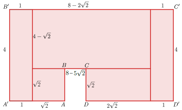
Example 4.2.

(Figure 17) The $\Pi$ -shaped octagon with $A^{\prime}B^{\prime}=4,B^{\prime}C^{\prime}=10-2\sqrt{2},AA^{\prime}=1+\sqrt{2},AB=\sqrt{2},DD^{\prime}=1+2\sqrt{2}$ can be tiled by 5 rectangles with rational aspect ratios, but cannot be tiled by less than 5 rectangles with rational aspect ratios.

Proof.

The tiling by 5 rectangles is shown in Figure 17. By Lemma 4.1, there exists a planar two-port circuit with $5$ edges $15,25,36,46,$ and $56$ of rational resistances such that $I_{1}=4,I_{2}=-\sqrt{2},I_{3}=\sqrt{2},I_{4}=-4,U_{1}-U_{2}=-(1+\sqrt{2}),U_{3}-U_{4}=-(1+2\sqrt{2}),U_{1}-U_{4}=-(1+\sqrt{2}),U_{3}-U_{4}=-(1+2\sqrt{2}),\Delta{U_{14}}:=U_{1}-U_{4},$ and $\Delta{U_{23}}:=U_{2}-U_{3}$ . This circuit satisfies the assumptions of Proposition 3.11.

Assume the converse: this octagon can be tiled by less than 5 rectangles with rational aspect ratios. Then, similarly to the previous paragraph, by Lemma 4.1 we get a two-port circuit with less than 5 edges and the same differences of the incoming voltages, the same voltage drop, and the same response. This contradicts to Proposition 3.11. ∎

5 Acknowledgments

I am grateful to my scientific advisor Mikhail Skopenkov for valuable discussions and help in writing and translating the paper. Also I would like to thank Pasha Pylyavskyy, who read this paper and provided ideas for further research.

References

[1] V. P. Bakalov, A. N. Ignatov, B. I. Kruk, Fundamentals of the theory of electrical circuits and electronics, Moscow, Radio and communication, 1989 (in Russian).
[2] A. C. Barlett, An extension of a property of artificial lines, Phil. Mag. 4:24 (1927), 902–907.
[3] L. A. Bessonov, Theoretical foundations of electrical engineering. Electric circuits - 11th ed., Revised and extended, Moscow, Gardariki, 2007 (in Russian).
[4] R. L. Brooks, C. A. B. Smith, A. H. Stone, and W. T. Tutte, The dissection of rectangles into squares, Duke Math. J. 7 (1940), 312–340.
[5] E. B. Curtis and J. A. Morrow, Inverse problems for electrical networks, Series on Appl. Math. 13, World Scientific, Singapore, 2000.
[6] M. Dehn, Über die Zerlegung von Rechtecken in Rechtecke, Math. Ann. 57 (1903), 314–332 (in German).
[7] R. Kenyon, Tilings and discrete Dirichlet problems, Israel J. Math. 105:1 (1998), 61–84.
[8] M. Prasolov, M. Skopenkov, Tiling by rectangles and alternating current, J. Combin. Theory A 118:3 (2011), 920-937.
[9] M. Skopenkov, V. Smykalov, A. Ustinov, Random walks and electric networks, Mat. Prosv. 3rd ser. 16 (2012), 25-47 (in Russian). Minor correction in: A. Yuryev, Random walks return, Mat. Prosv. 3rd ser. 20 (2016), 243-246.
[10] A. Zaslavsky, M. Skopenkov, A. Ustinov, Random walks and electric networks. In: Mathematics via Problems. Part 3: Combinatorics. Ed. by M. Skopenkov and A. Zaslavskiy. Transl. by P. Zeitz and S. Shubin, MSRI Mathematical Circles Library, MSRI and AMS, to appear.

Transformations of 2-port networks and tiling by rectangles

Abstract

1 Introduction

1.1 Transformations of two-port networks

1.2 Tilings

Theorem 1.1 (Dehn, 1903).

Theorem 1.2 (Kenyon, 1998).

Theorem 1.3.

Theorem 1.4.

1.3 Organization of the paper

2 Preliminaries

2.1 Electrical networks

Theorem 2.1.

Proposition 2.2.

Remark 2.3.

Proposition 2.4.

Corollary 2.5.

Proposition 2.6.

Corollary 2.7.

Theorem 2.8.

2.2 Two-port networks

Theorem 2.9.

Lemma 2.10.

Proof of Theorem 2.9.

Example 2.11.

Proof.

2.3 Electrical networks and tilings

Lemma 2.12.

3 Π\Pi-equivalence of two-port networks

Example 3.1.

Proof.

Proposition 3.2.

Proposition 3.3.

Theorem 3.4.

Proof.

Corollary 3.5.

Corollary 3.6.

Theorem 3.7.

Remark 3.8.

Remark 3.9.

Proof of Theorem 3.7.

Lemma 3.10.

Proof.

Proposition 3.11.

Proof.

Example 3.12.

4 Tilings of octagons

Lemma 4.1.

Proof.

Proof of Theorem 1.4.

Example 4.2.

Proof.

5 Acknowledgments

References

3 $\Pi$ -equivalence of two-port networks