Genomic Data Analysis using a Two Stage Expectation Propagation Algorithm for Analysis of Sparse Bayesian High-Dimensional Instrumental Variables Regression
Abstract
Simultaneous analysis of gene expression data and genetic variants is highly of interest, especially when the number of gene expressions and genetic variants are both greater than the sample size. Association of both causal genes and effective SNPs makes the use of sparse modeling of such genetic data sets, highly important. The high-dimensional sparse instrumental variables models are one of such useful association models, which models the simultaneous relation of the gene expressions and genetic variants with complex traits. From a Bayesian viewpoint, the sparsity can be favored using sparsity-enforcing priors such as spike-and-slab priors. A two-stage modification of the expectation propagation (EP) algorithm is proposed and examined for approximate inference in high-dimensional sparse instrumental variables models with spike-and-slab priors. This method is an adoption of the classical two-stage least squares method, to be used with the Bayes context. A simulation study is performed to examine the performance of the methods. The proposed method is applied to analysis of the mouse obesity data.
Keywords: Causal inference, Expectation propagation, Spike-and-Slab prior, Sparse instrumental variables model
1 Introduction
Detection of simultaneous association of gene expressions and single nucleotide polymorphism (SNP) with complex traits, such as obesity, heart disease and cancer, is one of the highly important issues in genome-wide studies (Emilsson, 2008). One of the useful models which provides a practical approach for jointly modeling the effects of genes and genetic markers on the trait as the response, is the instrumental variables (IV) method. IV models are extensively studied in econometrics literature (Heckman, 1977) and observational epidemiology and causal inference (see e.g. Lawlor, 2008, for a review until 2008). The high-dimensional sparse IV models are of interest in situations in which the number of covariates and instrumental variables are both greater than the sample size and there are too many zero coefficients (non-effective covariates and instrumental variables) in the model. Gautier & Tsybakov, 2011 proposed a Dantzig-type variable selection method for high-dimensional IV models. Belloni et al. , 2012 used the LASSO method (Tibshirani, 2011) for the first-stage covariates in a high-dimensional IV model. Recently, Lin et al. , 2015 have proposed a two-stage regularization method, by imposing the penalties to both coefficients of the covariates and instrumental variables in a high-dimensional IV model.
From a Bayesian viewpoint, the sparsity can be favored using sparsity-enforcing priors for the model coefficients. Recently, the sparse Bayesian models are widely applied in gene association studies for prediction and classification (Davies et al. , 2017; Yang et al. , 2017, e.g.,). The sparsity-enforcing priors are priors which are peaked at zero or have a large mass at zero. Laplace (Seeger, 2008), Student’s (Tipping & Faul, 2003), horseshoe (Carvalho et al. , 2009) and spike-and-slab (Mitchell & Beauchamp, 1988; Geweke, 1996; George & McCulloch, 1997) priors are some of the most important sparsity-enforcing priors. Among the aforementioned priors, the spike-and-slab priors are of a special interest, partly because of their mixture structure which allows to discriminate zero and non-zero coefficients, their closed-form convolution with Gaussian density, which makes the Gaussian approximation of the posteriors straightforward, and the less shrinkage effect on the non-zero coefficients induced by the spike-and-slab prior compared with the other priors.
Using the spike-and-slab priors, the posterior distribution can not be often computed algebraically and the approximation methods should be used to estimate the parameters of the model. Different asymptotically exact and approximate Bayesian inference are applied to sparse Bayesian models, such as Gibbs sampling (George & McCulloch, 1997; Hernández-Lobato et al. , 2015) variational Bayes (Attias, 1999; Carbonetto et al. , 2012) and expectation propagation (EP) algorithm (Nickisch & Rasmussen, 2008; Hernández-Lobato et al. , 2015). The EP algorithm (Minka, 2001) have many advantages over Gibbs sampling and variational Bayes, including less computational cost compared to Gibbs sampling and decreasing the probability of approximating local modes of the posterior compared to variational Bayes. Recently, Hernández-Lobato et al. , 2015 have proposed an EP method for linear regression models with spike-and-slab priors by splitting the posterior distribution into only three separate factors and approximating them separately. They have shown that the proposed method have a low computational cost and high precision with respect to other methods.
In this paper, we propose a two-stage modification of the EP method to Bayesian sparse high-dimensional IV models, with spike-and-slab prior. This proposed modification is based on the standard idea of replacing covariates by their expectations conditional on the instruments, as in the classical two-stage least squares (2SLS) method (Anderson, 2005), in which the covariates are first regressed on the instruments and the response is then regressed on the first stage predictors. A simulation study is conducted to examine the performance of the proposed method. We focus on the application of the proposed method to genetical genomic to identify potentially causal genes as covariates and genetic variants as instrumental variables.
The rest of this paper is organized as follows. Section 2 introduces the Bayesian modeling of the sparse instrumental variable model with spike-and-slab priors. The proposed two-stage modification of the EP algorithm is introduced and implemented to sparse IV model in Section 3. The numerical illustration including the simulation study and an analysis of the mouse obesity data is presented in Section 4, based on the proposed method. The details of the algorithm are given in the Appendix and the R functions to implement the proposed methods as well as other 2-stage sparse frequentist competitors are available at https://github.com/mortamini/2Stage-Sparse-IVR.
2 Materials and methods
2.1 The mouse obesity data set
Our aim is to analyze the mouse obesity data-set described by Wang et al. , 2006. The data-set includes an F2 intercross of 334 mice derived from the inbred strains C57BL/6J and C3H/HeJ on an apolipo-protein E (ApoE) null background, which were fed a high-fat Western diet from 8 to 24 weeks of age. The mice were genotyped using 1327 SNPs at an average density of 1.5 cM across the whole genome, and the gene expressions of the liver tissues of these mice were profiled on micro-arrays that include probes for 23,388 genes. Data on several obesity-related clinical traits were also collected on the animals. The genotype, gene expression, clinical data and the annotation table of genes are available for download, respectively, at Supplementary material of van Nas et al. , 2010 , National Center for Biotechnology Information Web site, Horvath’s Web page and the GSE2814 information page.
2.2 Sparse IV model with spike-and-slab priors
Suppose that , is a sample of size of scalar response variable , covariate vector (e.g. gene expressions), and vector of instrumental variables (e.g. genotypes). Consider the following IV model
| (1) |
for , where is a vector of unknown linear effects of the covariates, is a matrix of unknown linear effects of instrumental variables on the covariates, and are and vectors of random errors.
In order to consider the sparse high-dimensional IV model, we assume that both and are greater than and a large subset of coefficients in the vector and the matrix are zero. As considered by Lopes & Polson, 2014, we assume that are independent and identically distributed from -variate normal distribution with a zero vector mean and a variance-covariance matrix .
Hence, the likelihood function of and is
| (3) |
where is the matrix of covariates, is the vector of instruments and is a vector of responses.
To enforce the sparsity to the parameters and , we consider the spike-and-slab priors (Mitchell & Beauchamp, 1988; Geweke, 1996; George & McCulloch, 1997), which are mixtures of a normal density and a point probability mass at zero, as follows
| (4) |
| (5) |
where stands for the probability density function of the normal distribution with mean and variance , the hyper-parameters and take the values 0 (for zero coefficients) and 1 (for non-zero coefficients), is vectorised as , that is is formed by combining the rows of end to end. and are known variances and is the Dirac delta function, , if and , otherwise.
To develop a hierarchical Bayesian analysis, the priors for the hyper-parameter and are considered to be Bernoulli as follows
| (6) |
| (7) |
where and are known prior probabilities. These parameters are the main parameters for controlling the sparsity of the model and act like the penalty parameters in the frequentist penalized sparse model proposed by Lin et al. , 2015.
Given , and , the posterior of , , and is given by
| (8) |
where .
For a given new vector of , the predictive density of the response at a point is computed as follows
where the notations and stand for and , respectively.
2.3 A two stage modification of the EP algorithm
The Bayes approximation method EP (Minka, 2001) is an algorithm for approximation of the joint distribution of the parameters and the observed data with a simple distribution .
Let the likelihood function be with prior and the hyper-prior . The joint distribution of would be then
| (9) |
for a given number of factors . The aim of the EP algorithm is to approximate the components of the joint density , by , respectively. Each update step of the EP algorithm refines the parameters of , , so that the Kullback-Leibler (KL) divergence between the un-normalized distributions and is minimum, which is proved to have a single global solution (Bishop, 2016), where
and the KL divergence between and is
for the sigma-finite measure, .
Thus the EP algorithm is as follows:
-
1. Initialize parameters and hyper-parameters of and approximated factors, such that all priors and hyper-priors are noninformative.
-
2. Repeat until the parameters of converge:
-
2.1. For , select to be refined.
-
2.1.1. Compute ,
-
2.1.2. Update so that is minimized.
-
-
For the exponential family of distributions, the updated parameters of in step 2-1-2 are found by matching the sufficient statistics of and (Minka, 2001). Since the EP algorithm is not guaranteed to converge in general (Minka, 2001), it can be improved by damping the update operations of EP (Minka & Lafferty, 2002), in step , of the EP algorithm, by replacing by , where the damping parameter sequence is suggested to be a decreasing sequence, staring from a value near 1.
For Bayesian analysis of the sparse IV model (1) using the EP algorithm, first, we have to factorize the joint distribution of the parameters and the observed data, as in (9). In a similar strategy to that of Hernández-Lobato et al. , 2015, we factorized the joint distribution of the parameters and the observed data to only three factors as follows
where , and .
To imply the EP algorithm for approximation of the posterior function (8), one might consider the factorization (9) to the likelihood function (3), the priors (4) and (5), and the hyper-priors (6) and (7). Because of the complexity of the structure of the likelihood function , it is impossible to compute the sufficient statistics of , as needed in the EP algorithm for updating the parameters of the . Thus, implementation of the EP algorithm is intractable based on the full likelihood function (3). So, we propose a two-stage modification of the EP algorithm here, which uses the partial likelihoods in each stage instead of the full likelihood (3). This proposed modification is based on the standard idea of replacing covariates by their expectations conditional on the instruments, as in the classical two-stage least squares (2SLS) method (Anderson, 2005), in which the covariates are first regressed on the instruments and the response is then regressed on the first stage predictors. This method is also used by Lin et al. , 2015, who proposed a two stage regularization method for high-dimensional instrumental variables regression. Indeed, the simplification is done by replacing the complex covariance matrix with a diagonal matrix .
The structure of the two-stage EP is as follows:
- •
Stage I:
-
I-(ii): Factorize the joint distribution
(10) where , and .
-
I-(iii): Apply the EP algorithm to approximate the joint distribution in (10) by
(11) where
in which and are parameters to be estimated, and is the sigmoid function which guarantees the success probability of the Bernoulli distributions to be always in . Continue the EP algorithm until convergence. The estimate of is then obtained by the mean of the approximated posterior, that is
Then, compute the predicted covariate , in which .
- •
Stage II:
-
II-(ii): Factorize the joint distribution
(12) where , and .
-
II-(iii): Apply the EP algorithm to approximate the joint distribution in (12) by
(13) where
in which and are parameters to be estimated. Continue the EP algorithm until convergence.
The estimate of is then given by the mean of the approximated posterior, that is
To obtain final sparse estimates of and , we let
and
where is the th quantile of the vector .
- •
Finally, a post-estimation method is performed to obtain the final estimators using the ridge regression technique applied to the selected variables.
The details of the algorithm are given in the Appendix.
2.4 Initializing the model
In practice, the parameters and and the hyper-parameters , , and are unknown. The model can be initialized using one of the following strategies:
-
Strategy I: Initialize the model by first applying the 2-stage method of Lin et al. , 2015 to the data set along with a model selection criterion such as AIC or BIC to select the optimal model and obtain and , and then we initialize the model as follows
(14) (15) and
(16) where stands for the cardinality of the set , , is the squared norm of vector and is the squared Frobenius norm of matrix . This strategy is used in the simulation study, in Section 4.
3 Simulation study
In this section, a Monté Carlo simulation study is conducted, in order to examine the performance of the proposed method. For this purpose, the IV model with , , , and the following parameters is considered
where and stand for the vector of 1s and 0s with length , respectively, which means that
where and stand for the matrices of 1s and 0s, respectively. The vector is set such that 5% of its elements are non-zero, while this ratio is equal 1% for the vector . The number of repeated simulated data sets for the Monte Carlo simulation study is iterations. In each iteration:
- 1.
The genotype data, , is generated from Bernoulli distribution with a success probability of , for , , where s are generated from Beta distribution with parameters 3 and 7 (with mean 0.3 and standard deviation 0.138). This model tries to simulate a complicate phenomenon similar to the real genotype data which depends on Minor allele frequency (MAF) and Hardy-Weinberg Equilibrium.
- 2.
is generated from , for , ,
- 3.
is generated from , for .
The two-stage EP algorithm is applied in each iteration to estimate the parameters. As a result of the simulation study, the false negative rate and the false positive rate, defined as follows, are computed for estimation of and ,
and
where stands for the cardinality of the set .
Furthermore, 3-fold cross-validation (CV) criterion
are computed, where is a partition of .
The two-stage EP (2S.EP) method is compared with its two frequentist competitors proposed by Lin et al. , 2015, which are two-stage sparse IV model based on the LASSO (2S.LASSO) and SCAD (2S.SCAD) penalties. Figure 1 shows the box-plots of , , , , and the computation time for 2S.EP, 2S.LASSO and 2S.SCAD. As one can see from Figure 1, the 2S.EP method performs better than 2S.LASSO and 2S.SCAD, in detecting the effective and non-effective covariates (In terms of FPR and FNR), while it has a poor prediction performance and more computation time relative to the frequentist methods 2S.LASSO and 2S.SCAD.

4 Analysis of mouse obesity data
After the individuals, SNPs, and genes with a missing rate greater than 0.1 were removed, the remaining missing genotype and gene expression data were imputed using the linkage based imputation method (Xu et al. , 2015) and nearest neighbor averaging (Troyanskaya et al. , 2001), respectively. Merging the genotype, gene expression, and clinical data yielded a complete data-set with SNPs and genes on mice. To enhance the interpretability and stability of the results, we focus on the genes that have standard deviation of gene expression levels greater than . The latter criterion is reasonable because gene expressions of too small variation are typically not of biological interest and suggest that the genetic perturbations may not be sufficiently strong for the genetic variants to be used as instruments.


Our goal is to jointly analyze the genotype, gene expression, and clinical data to identify important genes related to body weight.
The two-stage EP algorithm (2S.EP), proposed in the previous section, as well as the two-stage LASSO (2S.LASSO) and SCAD (2S.SCAD) methods, proposed by Lin et al. , 2015, are applied to the mouse obesity data-set. For the two-stage EP algorithm, Strategy II is used to initialize the hyper-parameters, using the 3-fold cross-validation as the criterion and the maximum errors for both stages was . Figure 2 shows the 3D plot of 3-fold cross-validation as a function of and . The values of and are selected from the sequence from 0.1 to 0.9 with steps of 0.2. The optimal values are and .
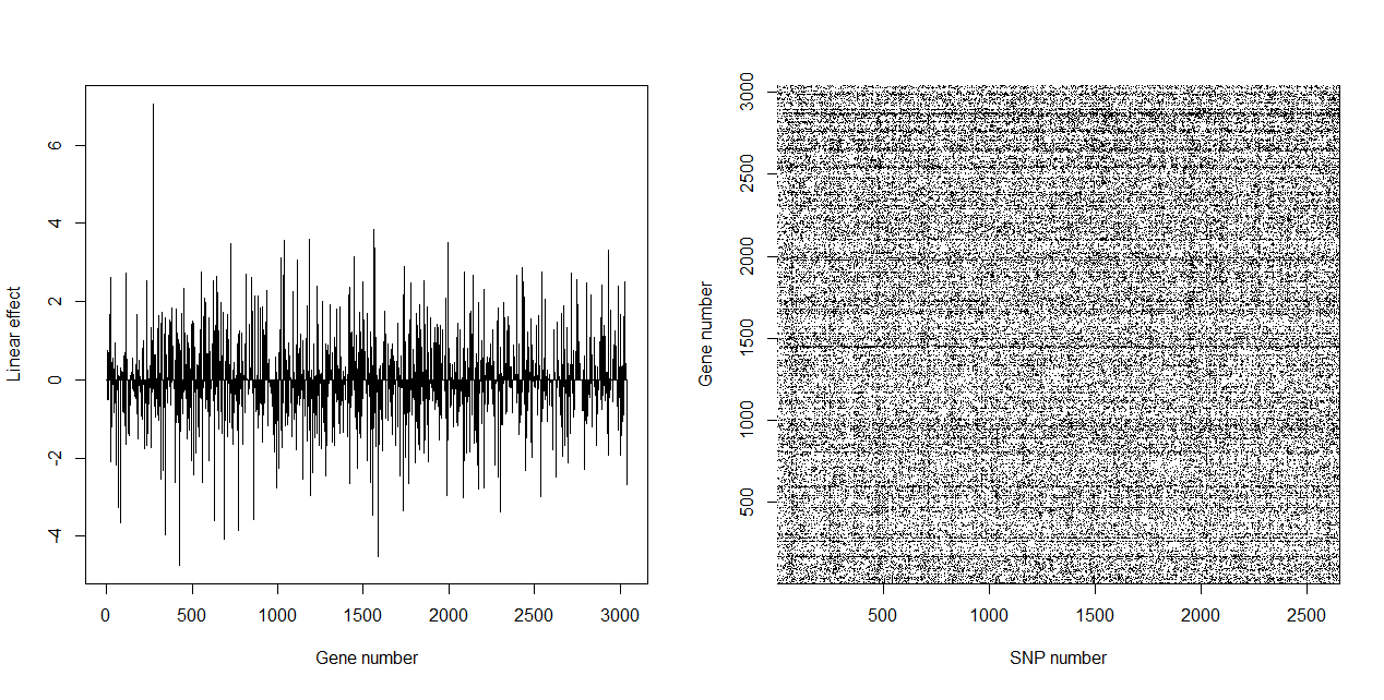
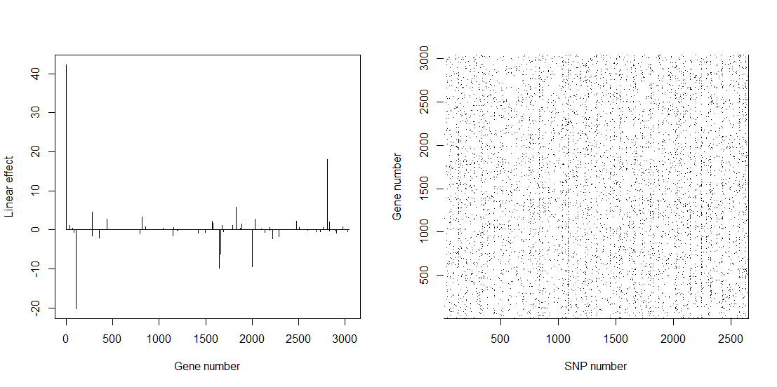
Figure 3 shows the sparse estimates of the coefficients (left) and (right) for the mouse obesity data-set, based on the two stage EP (up) LASSO (middle) and SCAD (down) methods. The values of the non-zero effects of the genes (covariates) on the response can be seen from the left panel of Figure 3, while in the right panel, a 2D sparse plot of the estimate of the coefficient matrix is shown. The black dots and lines represent the non-zero estimates. The exact estimates as well as the effective genes and SNPs are available at https://github.com/mortamini/2Stage-Sparse-IVR.
Based on the obtained estimates, the coefficient of determination for prediction of the response given , , the 3-fold cross-validation, CV, and the Bayesian Information Criterion, , are given in Table 1. As one can see from Table 1, the 2S.EP method is preferred based on the BIC criterion, while the 2S.LASSO method has a lower CV.
| method | CV | ||
|---|---|---|---|
| 2S.EP | 0.99 | 5.27 | 17079 |
| 2S.LASSO | 0.61 | 4.19 | 18161 |
| 2S.SCAD | 0.84 | 4.67 | 17898 |
5 Concluding remarks
The causal inference using the Bayes method and based on the sparsity-enforcing priors is considered in this paper and the EP method is used for approximation of the posterior distribution. An advantage of using the Bayesian causal inference is that the posterior distribution of the estimators are obtained. Also, the results of the simulation study shows that the 2S-EP method performs better than 2S.LASSO and 2S.SCAD, in detecting the effective and non-effective covariates.
The R functions to implement the proposed methods as well as other 2-stage sparse frequentist competitors are available at https://github.com/mortamini/2Stage-Sparse-IVR. The post estimation is also considered in the prepared functions, which is re-estimation of the model parameters after removing the ineffective covariates from the model, using frequentist ordinary or Ridge models. The execution time of the codes should be improved by calling C routines within the R codes for the EP algorithm in each stage, and by using parallel programming.
It is worth noting that the proposed results of this paper could be improved by further cross-validation over all parameters of the model, which was ignored for the matter of time.
Acknowledgements
The author would like to thank the anonymous referee for his/her valuable comments and suggestions on an earlier version of this article, which significantly improved the paper. This research was partially support by Iranian National Science Foundation under the grant number 99009577.
Appendix (details of the algorithm)
Using the product rule of the normal and Bernoulli densities, and by considering the normalizing constants, the approximated posterior distributions obtained from (11) and (11) are
| (17) |
and
| (18) |
respectively, where, for and ,
Thus, for and , final non-sparse estimates of and are and , respectively. For the purpose of variable selection and obtaining the sparse estimates, one can let , if , and , if , for suitable threshold values,
With an adapted approach to that used in Hernández-Lobato et al. , 2015, one can show that, in the first step of both EP algorithms, in two stages, the parameters of and are updated and do not change in the next steps, as follows
Furthermore, in step , , the parameters of and are updated in step , for and , as
where for and
To avoid the updated values of the parameters and to be negative, Hernández-Lobato et al. , 2015 suggest to update the parameters of and by minimizing
under the constraint , , respectively, and proved that this will result if infinite optimal value of and . Thus, whenever each of these parameters get negative, we simply replace them by a large positive constant.
The update of the parameters of is again similar to that of Hernández-Lobato et al. , 2015, while that of , is somehow different from that of Hernández-Lobato et al. , 2015, partly because of the -variate normal density component in . For , letting and be the diagonal matrices with diagonal elements and , respectively, the updated parameters of and in step of the EP algorithms, for and , are
where
and stands for the Kronecker product.
In many problems, especially for the genetic association problems, and are large values, and thus computation of the updated matrix and vector in step of the EP algorithm needs huge amount of memory. To reduce the used memory for each computation and provide suitable formulas for parallel computations, one can use the fact that , , and are block diagonal matrices and decompose the computations into the following sub-computations
for , where stand for the th diagonal block of the diagonal matrix , and is the th row of the matrix .
References
- Anderson, (2005) Anderson, TW. 2005. Origins of the limited information maximum likelihood and two-stage least squares estimators. Journal of Econometrics, 127(1), 1–16.
- Attias, (1999) Attias, H. 1999. Inferring parameters and structure of latent variable models by variational Bayes. Pages 21–30 of: Proceedings of the Fifteenth conference on Uncertainty in artificial intelligence. Morgan Kaufmann Publishers Inc.
- Belloni et al. , (2012) Belloni, Alexandre, Chen, Daniel, Chernozhukov, Victor, & Hansen, Christian. 2012. Sparse models and methods for optimal instruments with an application to eminent domain. Econometrica, 80(6), 2369–2429.
- Bishop, (2016) Bishop, C.M. 2016. Pattern Recognition and Machine Learning. Information Science and Statistics. Springer New York.
- Carbonetto et al. , (2012) Carbonetto, Peter, Stephens, Matthew, et al. . 2012. Scalable variational inference for Bayesian variable selection in regression, and its accuracy in genetic association studies. Bayesian analysis, 7(1), 73–108.
- Carvalho et al. , (2009) Carvalho, C. M., Polson, N. G., & Scott, J. G. 2009. Handling sparsity via the horseshoe. Pages 73–80 of: International Conference on Artificial Intelligence and Statistics.
- Davies et al. , (2017) Davies, Vinny, Reeve, Richard, Harvey, William T, Maree, Francois F, & Husmeier, Dirk. 2017. A sparse hierarchical Bayesian model for detecting relevant antigenic sites in virus evolution. Computational Statistics, 1–41.
- Emilsson, (2008) Emilsson, V., et al. 2008. Genetics of gene expression and its effect on disease. Nature, 452(7186), 423–428.
- Gautier & Tsybakov, (2011) Gautier, E., & Tsybakov, A. 2011. High-dimensional instrumental variables regression and confidence sets. arXiv preprint arXiv:1105.2454.
- George & McCulloch, (1997) George, E. I., & McCulloch, R. E. 1997. Approaches for Bayesian variable selection. Statistica sinica, 339–373.
- Geweke, (1996) Geweke, John. 1996. Variable selection and model comparison in regression. In Bayesian Statistics 5.
- Heckman, (1977) Heckman, James J. 1977. Dummy endogenous variables in a simultaneous equation system.
- Hernández-Lobato et al. , (2015) Hernández-Lobato, J. M., Hernández-Lobato, D., & Suárez, A. 2015. Expectation propagation in linear regression models with spike-and-slab priors. Machine Learning, 99(3), 437–487.
- Lawlor, (2008) Lawlor, Debbie A et al. 2008. Mendelian randomization: using genes as instruments for making causal inferences in epidemiology. Statistics in medicine, 27(8), 1133–1163.
- Lin et al. , (2015) Lin, Wei, Feng, Rui, & Li, Hongzhe. 2015. Regularization methods for high-dimensional instrumental variables regression with an application to genetical genomics. Journal of the American Statistical Association, 110(509), 270–288.
- Lopes & Polson, (2014) Lopes, Hedibert F, & Polson, Nicholas G. 2014. Bayesian instrumental variables: priors and likelihoods. Econometric Reviews, 33(1-4), 100–121.
- Minka & Lafferty, (2002) Minka, Thomas, & Lafferty, John. 2002. Expectation-propagation for the generative aspect model. Pages 352–359 of: Proceedings of the Eighteenth conference on Uncertainty in artificial intelligence. Morgan Kaufmann Publishers Inc.
- Minka, (2001) Minka, Thomas Peter. 2001. A family of algorithms for approximate Bayesian inference. Ph.D. thesis, Massachusetts Institute of Technology.
- Mitchell & Beauchamp, (1988) Mitchell, Toby J, & Beauchamp, John J. 1988. Bayesian variable selection in linear regression. Journal of the American Statistical Association, 83(404), 1023–1032.
- Nickisch & Rasmussen, (2008) Nickisch, Hannes, & Rasmussen, Carl Edward. 2008. Approximations for binary Gaussian process classification. Journal of Machine Learning Research, 9(Oct), 2035–2078.
- Seeger, (2008) Seeger, Matthias W. 2008. Bayesian inference and optimal design for the sparse linear model. Journal of Machine Learning Research, 9(Apr), 759–813.
- Tibshirani, (2011) Tibshirani, Robert. 2011. Regression shrinkage and selection via the lasso: a retrospective. Journal of the Royal Statistical Society: Series B (Statistical Methodology), 73(3), 273–282.
- Tipping & Faul, (2003) Tipping, M. E., & Faul, A. C. 2003. Fast marginal likelihood maximisation for sparse Bayesian models. In: AISTATS.
- Troyanskaya et al. , (2001) Troyanskaya, O., Cantor, M., Sherlock, G., Brown, P., Hastie, T., Tibshirani, R., Botstein, D., & Altman, R. B. 2001. Missing value estimation methods for DNA microarrays. Bioinformatics, 17(6), 520–525.
- van Nas et al. , (2010) van Nas, Atila, Ingram-Drake, Leslie, Sinsheimer, Janet S, Wang, Susanna S, Schadt, Eric E, Drake, Thomas, & Lusis, Aldons J. 2010. Expression quantitative trait loci: replication, tissue-and sex-specificity in mice. Genetics, 185(3), 1059–1068.
- Wang et al. , (2006) Wang, S., Yehya, N., Schadt, E. E., Wang, H., Drake, T. A., & Lusis, A. J. 2006. Genetic and genomic analysis of a fat mass trait with complex inheritance reveals marked sex specificity. PLoS genetics, 2(2), e15.
- Xu et al. , (2015) Xu, Y., Wu, Y., Gonda, M. G., & Wu, J. 2015. A linkage based imputation method for missing SNP markers in association mapping. Journal of Applied Bioinformatics & Computational Biology, 4(1).
- Yang et al. , (2017) Yang, Aijun, Jiang, Xuejun, Shu, Lianjie, & Lin, Jinguan. 2017. Bayesian variable selection with sparse and correlation priors for high-dimensional data analysis. Computational Statistics, 32(1), 127–143.