Time-Average Convergence in a Generalization of Multiagent Zero-Sum Games
Abstract
We introduce a generalization of zero-sum network multiagent matrix games and prove that alternating gradient descent converges to the set of Nash equilibria at rate for this set of games. Alternating gradient descent obtains this convergence guarantee while using fixed learning rates that are four times larger than the optimistic variant of gradient descent. Experimentally, we show with 97.5% confidence that, on average, these larger learning rates result in time-averaged strategies that are 2.585 times closer to the set of Nash equilibria than optimistic gradient descent.
1 Introduction
We study online learning algorithms applied to network matrix games in the form
These games are used to capture a network where an agent receives utility based on their interactions with other agents, e.g., agent receives utility when agent selects action and agent selects action . A solution to this game is known as a Nash equilibrium, , and is given by
i.e., no agent can obtain a better outcome by deviating from .
Zero-sum network games, equivalently zero-sum polymatrix games [9], are a special case where for all pairs of agents – equivalently, . Online learning dynamics and algorithms in zero-sum games have received a great deal of attention due to their numerous applications in areas such as Generative Adversarial Networks (GANS) [16], bargaining and resource allocation problems [25], and policy evaluation methods [14].
In each of these settings, the goal is to find a Nash equilibrium via online optimization techniques by having agents repeatedly play the game while updating their actions using only information about cumulative payouts, i.e., agent has access to only when selecting strategy where is agent ’s action in the -th game. While there are methods that guarantee last-iterate convergence (e.g., [12, 27, 1]), most methods focus on time-average convergence () since these methods tend to be faster (see e.g., [15]).
The standard strategy for establishing time-average convergence relies on a connection between convergence and regret, a standard measure of performance in online optimization. Specifically, agent ’s regret for not playing is the difference between ’s cumulative utility and the cumulative utility had played instead. Formally . It is well-known that time-average regret for all agents implies time-average convergence to the set of Nash equilibrium in bounded zero-sum games (see [10]).
While there are several algorithms that obtain time-average regret and convergence for zero-sum games [19, 23], no such results are known for general-sum games (no restrictions on ). Recently, time-average regret has been shown in general-sum games [13]. However, this is insufficient for quickly finding Nash equilibria; time-average regret in these settings only implies time-average convergence to the set of coarse correlated equilibria – a significantly weaker solution concept.
To provide finer distinctions between the types of games, [20] introduces a hierarchy to capture all games. In the two agent settings, the rank of game is denoted by implying a two-agent game is zero-sum if and only if it is rank-0. Standard algorithms for finding Nash equilibria in zero-sum games are known to not work well even in rank-1 games [7] and other fast methods to find Nash equilibria for rank-1 games have been developed [2]. In this paper, we focus on fast time-average convergence for a different generalization of zero-sum games.
1.1 Our Motivations
Our methodology is heavily motivated by continuous-time optimization in games where agents’ strategies are a continuous function of other agents’ actions (see e.g., [22]). In particular, continuous-time variants of follow-the-regularized-learner algorithms (FTRL), e.g., gradient descent and multiplicative weights, are known to achieve time-average regret in general-sum games [21]. In the setting of zero-sum games, these learning dynamics maintain constant energy and cycle around the set of Nash equilibria [21] on closed orbits.
However, this is drastically different than what we see from discrete-time FTRL where agent strategies diverge from the set of Nash equilibria [4]. This is because these algorithms are poor approximations of the continuous-time dynamics. Continuous-time variants of FTRL have been shown to form a Hamiltonian dynamic [6], a well-known concept used to capture the evolution of a physical system. Discrete-time FTRL can be formulated by applying Euler integration to this Hamiltonian system; regrettably Euler integration is well-known to be a poor approximator of Hamiltonian systems. Instead, we focus on symplectic integrators (see e.g., [17, 18]), which were designed for Hamiltonian systems. Specifically, we study alternating gradient descent, which arises naturally by applying Verlet integration, a symplectic technique, to continuous-time gradient descent.
1.2 Our Contributions
We prove that multi-agent alternating gradient descent achieves time-average convergence to the set of Nash equilibrium in network zero-sum games (Theorem 5.10) matching the best known bound for convergence in zero-sum games. We show that alternating gradient descent accomplishes the convergence guarantee with learning rates up to four times larger than optimistic gradient descent. Our theoretical work suggests that these larger learning rates translate to faster optimization guarantees (Theorems 3.4 and 3.5). Our experiments support this; experimentally we show with 97.5% confidence that, on average, alternating gradient descent results in time-averaged strategies that are 2.585 times closer to the set of Nash equilibria than optimistic gradient descent.
Moreover, we introduce a generalization of the zero-sum network games, and show alternating gradient descent also achieves time-average convergence to the set of Nash equilibria. In this generalization, we allow each agent to multiply their payoff matrices by an arbitrary positive-definite matrix. Formally, a network positive negative definite game is given by
| where is positive-definite | |||
Our proposed methods allow us to extend important convergence results to settings that are adversarial in nature, but not necessarily zero-sum. We remark that our generalization is distinct from the rank-based hierarchy of bimatrix games introduced by [20]. Specifically, the set of positive-negative definite games includes games at every level of the hierarchy. Further, unlike zero-sum games, an agent’s payoff reveals no information about the payoff of other agents – even in the 2-agent case.
We accomplish this by showing that alternating gradient descent behaves similarly to its continuous-time analogue. Specifically it has (i) an invariant energy function capturing all updates (Theorem 5.8), (ii) these energy functions are bounded (Theorem 4.8) and (iii) strategies approximately cycle (Theorem 4.7). Finally, we relate the time-average of the strategies directly to the cyclic nature of the algorithm to prove time-average convergence.
In addition, we also prove several important properties of alternating gradient descent in general-sum games. Most notably, an agent using alternating gradient descent has regret after agent 1 updates regardless of the opponents’ strategies (Theorem 5.6). We remark that alternating gradient descent is unique relative to other learning algorithms in that agents take turns updating; as such, agent 1’s regret is not necessarily after other agents update and therefore Theorem 5.6 cannot be directly compared to regret guarantees for other algorithms, e.g., [13] remains the best guarantee for the standard notion of regret in general-sum games.
2 Preliminaries
We study repeated matrix network games between agents where each agent receives utility based on their interactions with other individual agents. Agent ’s set of available actions are given by a convex space . For most of this paper, we use for some positive integer . Once selecting strategies, , agent receives a utility of for the interaction between agents and where . This yields the following network game where each agent seeks to maximize their individual utilities.
| (Network Matrix Game) |
The term denotes agent ’s payoff matrix against agent . A solution to this game is known as a Nash equilibrium, , and is characterized by
| (A Nash Equilibrium) |
i.e., no agent can obtain a better outcome by deviating from . When is affine and full-dimensional, an equivalent condition for a Nash equilibrium is given by since otherwise agent could move their strategy in the direction to increase their utility. Therefore is a Nash equilibrium if and only if for each agent . When , as is this case in most of this paper, always corresponds to a Nash equilibrium. However in Section 6 we extend our results to the utility function where Nash equilibria can be arbitrarily located.
In addition to general-sum games (no restrictions on ), we also consider two other standard types of games – zero-sum and coordination games.
Definition 2.1.
A network game is a zero-sum network game iff for all .
Definition 2.2.
A network game is a coordination network game iff for all .
In a zero-sum network game, agent loses whatever agent gains from their interaction. By [9] every zero-sum polymatrix game (a multiagent game where payouts are determined by tensors) is a zero-sum game and we lose no generality by replacing every instance of “zero-sum game” with “zero-sum polymatrix game”. At the other end of spectrum, agent and agent always have the same gains from their interactions in a coordination game. While our main results are for generalizations of zero-sum games, we also include several results for general-sum games and a generalization of coordination games.
2.1 Online Optimization in Games
Our primary interest is in repeated games. In this setting, each agent selects a sequence of strategies and agent receives a cumulative utility of . In most applications, is selected after seeing the gradient of the payout from the previous iteration, i.e., after seeing . Gradient descent (Algorithm SimGD) is one of the most classical algorithms for updating strategies in this setting.
The learning rate describes how responsive agent is to the previous iterations. Typically in applications of Algorithm SimGD, decays over time in order to prove time-average regret and convergence when is compact. However, this decaying learning rate may not be necessary in general; [5] shows the same guarantees in 2-agent, 2-strategy zero-sum games with an arbitrary fixed learning rate and provides experimental evidence to suggest the results extend to larger games. In this paper, we consider variations of gradient descent in order to improve optimality and convergence guarantees. The variants we consider all rely on time-invariant learning rates that are independent of the time horizon and yield stronger optimization than the classical method of gradient descent with simultaneous updates.
3 Alternating Gradient Descent in 2-Agent Games
We begin by closely examining a 2-agent game. For reasons which will become apparent later, we will simplify the notation so that describes agent ’s strategy space, describes agent 2’s strategy space, and and describe the agent’s payoff matrices respectively. This results in the following game.
| (2-Agent Game) | |||
In this section, we analyze alternating gradient descent (Algorithm 2AltGD below) in 2-agent games and show four properties for general-sum games:
- 1.
Regret: An agent has time-average regret immediately after updating if they use alternating gradient descent with an arbitrary vector of fixed learning rates against an arbitrary opponent with an unknown time horizon (Theorem 3.2). We remark that the guarantee does not hold after the opposing agent updates (Proposition 3.3).
- 2.
- 3.
Self-Actualization: In order to maximize agent ’s regret for not playing the fixed strategy , agent two will actually force agent 1 to play the strategy . Formally, for any sequence that maximizes agent 1’s regret for using from alternating gradient descent instead of the fixed strategy will result in (Theorem 3.6).
- 4.
Volume Preservation: Alternating gradient descent preserves the volume of every measurable set of initial conditions when agents use arbitrary learning rates (Theorem 3.7).
We show and explore the meaning of each of these properties in Sections 3.1–3.4 respectively. Unlike standard analyses in online optimization, we prove our results for a generalized notion of learning rates. Specifically, we allow individual agents to use different learning rates for each individual strategy. For instance, suppose an agent fundamentally believes that the strategy “rock” is the most important strategy in the game rock-paper-scissors. Then they may wish to use a larger learning rate for rock relative to scissors, e.g., a learning rate of and . In this case, if an agent observes a benefit of 1 for both rock and scissors, then the agent will increase their weight for rock by while only increasing their weight for scissors by . For a single agent, we do not see an immediate algorithmic benefit of using different learning rates and therefore make no suggestion for it in practice. However, this generalization will be important for extending our results to multiagent systems in Section 5. We also remark that [3] proves (1) using a scalar learning rate and (4) in the setting of only zero-sum games using a scalar learning rate.
We begin by presenting Algorithm 2AltGD for alternating gradient descent between 2 agents. In Algorithm 2AltGD, represents a diagonal matrix where the diagonal is populated by the vector of learning rates . Similarly, can be expressed by the Hadamard product indicating that the th strategy is weighted according to . However, for notation purposes, it will be simpler to work with the diagonal matrix . We also remark that for all of our analysis that can be replaced with an arbitrary positive-definite matrix.
Remark 3.1.
3.1 Time-Average Regret
In traditional algorithmic settings, where agents update simultaneously, agent 1’s regret with respect to a fixed strategy is defined as
| (Standard Notion of Regret for Simultaneous Updates) |
i.e., the difference between the utility agent 1 would receive if the fixed strategy was played against and the utility agent 1 received by playing the sequence . Regret is the standard notion used to understand the performance of algorithms in repeated games and in online optimization in general. In the setting of bounded zero-sum games, it is well-known that the time-average of the strategies converges to the set of Nash equilibria whenever regret grows at rate (sublinearly). Generally in online optimization, if regret grows at rate , then the time-average regret converges to zero implying that, on average, the algorithm performs as well as the fixed strategy .
In the setting of alternating play where agents take turns updating, agent 2 plays the strategy twice – once in the th iteration when agent 2 updates () and once when agent 1 updates in the th iteration (). As such, we update the notion of regret accordingly:
| (Regret After Agent 1 Updates) |
From an economic standpoint, it makes sense that agents would receive utility after each update. If agents only received utility after both agents updated, then the agent that updates last would decidedly have an advantage since they would see the other agent’s strategy. As such, no rational agent would agree to take turns updating unless they receive utility every time they update. We remark that this notion of regret only captures agent 1’s regret after 1 updates and is not sufficient on its own to guarantee time-average convergence. We discuss the implication of this definition at the end of this section.
Theorem 3.2.
If agent 1 updates their strategies with Algorithm 2AltGD with an arbitrary vector of fixed learning rates , then agent 1’s time-average regret with respect to an arbitrary fixed strategy after updating in iteration is , regardless of how their opponent updates. More specifically, agent 1’s total regret is exactly
Proof.
The total regret for agent 1 after agent 1 updates in iteration is
where the first equality follows from line 3 of Algorithm 2AltGD, the second equality follows since is symmetric, the third equality follows by canceling out terms from the telescopic sum, and where the inequality follows since the function has a critical point at , which corresponds to a global maximum since is positive-definite. Dividing the above equations by yields that the time-average regret is in . ∎
Theorem 3.2 implies that agent 1’s regret does not grow at all. This suggests that agent strategies will quickly converge to optimality in zero-sum games; we formally show this in Section 4. Interestingly, this result implies that we can compute agent 1’s regret using very small amount of information. Specifically, we only need to know agent 1’s first and last strategy (with no information about agent 2) to compute their total regret.
While this bound on regret is incredibly powerful – it holds regardless of how the opponent updates and for any learning rate – the guarantee does not necessarily hold if regret is computed after agent 2 updates. As demonstrated in the proof of Proposition 3.3, agent 2 can make their final strategy arbitrarily large in order to make agent 1’s regret arbitrarily large. However, in practice, we do not necessarily expect agent 2 to play large strategies; for instance in Section 4, we show that is bounded when both agents use alternating gradient descent in zero-sum games. This implies that agent 1 has bounded regret even when regret is computed after agent 2 updates (Corollary 4.9).
Proposition 3.3.
Suppose is invertible. If agent 1’s regret is computed after agent 2 updates, then agent 1’s regret with respect to can be made arbitrarily large if .
Proof.
After agent updates, agent 1’s regret is given by
Let . Then agent 1’s regret after agent 2 updates approaches infinity as . ∎
3.2 An Argument for Large Learning Rates
In most settings of online optimization, small learning rates are used to prove optimization guarantees. However, in this setting we actually show that a large learning rate yields stronger lower bounds on the utility gained.
Theorem 3.4.
Agent 1’s total utility after updating in the iteration is .
Proof.
Following identically to the proof of Theorem 3.2,
The lower bound follows since is positive-definite implying . ∎
Recalling that is positive-definite, the bound and converges to as the learning rate grows large, i.e., by using an arbitrarily large learning rate, an agent can guarantee that they lose arbitrarily little utility. This is contrary to most online learning algorithms that suggest small, relatively unresponsive learning rates from agents. Admittedly, Theorem 3.4 only provides a lower bound that depends on the learning rates and says little about the cumulative utility as a function of the learning rate . However, in Theorem 3.5, we show that an agent is better served with large learning rates when playing against an unresponsive agent.
Theorem 3.5.
If agent 1 is playing against an oblivious, non-equilibrating opponent – i.e., if is independent of and – then agent 1 can make their utility arbitrarily high after updating in the iteration by making arbitrarily high.
Proof.
Agent 1’s total utility is
thereby completing the proof of the theorem. ∎
3.3 Self-Actualization
Next, we show that in order to maximize agent 1’s regret for not playing , Algorithm 2AltGD will actually force agent 1 to play . We refer to this property as self-actualization. Once agent 1 regrets not playing the strategy as much as possible, the agent will realize that strategy.
Theorem 3.6.
Suppose agent 1 updates their strategies with Algorithm 2AltGD. If the opponent’s actions maximize agent 1’s regret after agent 1 updates in the iteration for not playing the fixed strategy , then .
Ordinarily, we would have to be quite careful in making this claim and trying to prove it. Altering the sequence alters agent 1’s sequence and there it seems difficult to explicitly give a sequence that maximize agent 1’s regret. However, the proof of Theorem 3.2 is quite strong – the total regret relies only on and . The proof of Theorem 3.6 follows immediately from Theorem 3.2 since the upper bound was found using the unique optimizer .
3.4 Conservation of Volume in general-sum games
In this section, we examine the volume expansion/contraction properties of Algorithm 2AltGD. Formally, let be a measurable set of initial conditions and let be the set obtained after updating every point in with Algorithm 2AltGD (see Figure 1). Formally, . We compare the volume of to ; specifically, we show that this volume is invariant.


On its own, volume conservation is nice stability property due to its close connection with Lyapunov chaos. Lyapunov chaos refers to a phenomenon in dynamical systems where a small perturbation in initial conditions may result in arbitrarily different dynamical systems. Specifically, volume expansion implies that a small perturbation to the initial conditions can result in drastically different trajectories. Formally, let be a relatively small measurable set of initial conditions. If the volume of goes to infinity, then there exists an iteration and two points and that are arbitrarily far apart. However, by definition of , and evolve from and . This implies the two points, despite being close together initially, will diverge from one another over time.
We show that alternating gradient descent is volume preserving in general-sum 2-agent games.
Theorem 3.7.
Algorithm 2AltGD is volume preserving for any measurable set of initial conditions.
Proof.
Algorithm 2AltGD can be expressed as the two separate updates below.
| (Line 3 of Algorithm 2AltGD) | ||||
| (Line 4 of Algorithm 2AltGD) |
To show that the combined updates preserve volume, it suffices to show that each individual update preserves volume. Thus, it suffices to show that the absolute value of the determinant of the Jacobian for each update is 1 [26, Theorem 7.26]. The Jacobians for the updates are
| (Line 3 Jacobian) | |||
| (Line 4 Jacobian) |
where and are the identity matrices with the same dimension as and respectively.
Since both Jacobians are block triangular with zeros on the subdiagonal and superdiagonal respectively, their corresponding determinants are and therefore Algorithm 2AltGD preserves volume when updating a measurable set of strategies thereby completing the proof. ∎
Remark 3.8.
Volume conservation holds even if agents’ learning rates change overtime () since the determinant of the Jacobian is independent of .
Thus, alternating gradient descent preserves volume. This is in contrast to the standard implementation of gradient descent (Algorithm SimGD) where volume expands in zero-sum games (see [11] and Figure 2).

Regrettably however, volume conservation is insufficient to avoid Lyapunov chaos; in Lemma 3.9, we show that two points can still move arbitrarily far apart in the setting of a coordination game as depicted in Figure 3.


Lemma 3.9.
Let and with . The volume of is 4 while the diameter of is in where is the golden-ratio.
4 2-Agent Positive-Negative Definite (Zero-Sum) Games
In this section, we introduce a new class of games that includes all zero-sum games and show that Algorithm 2AltGD results in strategies that are bounded (Theorem 4.8), are Poincaré recurrent (Theorem 4.7), and have time-average convergence to the set of Nash equilibria (Theorem 4.11). Specifically, we study a generalization of zero-sum games that allows each agent to multiply their payoff matrices by arbitrary positive definite matrices and respectively, i.e., and for all .
| (Positive-Negative Definite Game) | ||||
We remark that recurrence (Theorem 4.7) and bounded orbits (Theorem 4.8) were shown for zero-sum games (without positive definite transformations) with a scalar learning rate in [3]. Unlike the results for regret in Theorem 3.2, arbitrary learning rates are not allowed – to obtain time-average convergence, the learning rates must be sufficiently small. Importantly, we show that Algorithm 2AltGD allows four times larger learning rates than required for optimistic gradient descent.
4.1 Importance of Positive-Negative Definite Games
Zero-sum games are only a measure zero set of positive-negative definite games and therefore our results drastically expand the applications of learning algorithms. This is particularly important for many economic settings where the underlying games are somewhat adversarial but not necessarily zero-sum. In such settings, it is currently unknown whether results for zero-sum games extend and thus, the best known for an algorithm in a similar setting is poly time-average convergence to the set of coarse correlated equilibria [13] – a class of equilibria significantly less important than the set of Nash equilibria. We introduce techniques to show that Algorithm 2AltGD results in time-average convergence to the set of Nash equilibria (Theorem 4.11) in this setting. We remark that the proof techniques we introduce can likely be used to extend many results for zero-sum games to positive-definite transformations of zero-sum games for other algorithms, e.g., optimistic gradient descent.
Unlike zero-sum games, in (Positive-Negative Definite Game) agent 1’s utility function uncovers no information about agent 2’s utility function. In contrast, in a zero-sum game, agent 1 always has knowledge of agent 2’s payout and can directly compute the set of Nash equilibria as a result. As shown in Proposition 4.1, it is impossible for agent 1 to independently determine a Nash equilibrium in a positive-negative definite game.
Proposition 4.1.
Unlike zero-sum games, agent 1 cannot determine the set of Nash equilibria with access only to agent 1’s payoff matrix in (Positive-Negative Definite Game).
Proof.
To prove the proposition, we give two different games and where agent 1 has the same payoff matrix in both games () but where agent 1’s set of Nash equilibria are different in each game.
| (Matrices for First Game) |
With respect to this game, implying agent 2’s set of Nash equilibria is . Similarly, implying agent 1’s set of Nash equilibria is .
| (Matrices for Second Game) |
With respect to this game, and agent 2’s Nash equilibria are unchanged. However, implying agent 1’s set of Nash equilibria are . ∎
Remark 4.2.
The game introduced in the proof of Proposition 4.1 is necessarily degenerate; since is always a Nash equilibrium, for two games to have a different set of Nash equilibria one game must have multiple Nash equilibria. In Section 6, we extend our results to a generalization of bimatrix games that allows for an arbitrary unique Nash equilibrium. It is then straightforward to extend Proposition 4.1 using two non-degenerate games.
4.2 Using the Correct Basis
The adversarial nature of (Positive-Negative Definite Game) is better revealed when examining the game in the bases induced by the transformations and . As such, we introduce the notion of a weighted normal to simply our proofs.
Definition 4.3.
Let be a positive definite matrix ( and for all ). Then the weighted-norm of the vector with respect to is .
Weighted norms are often used in physics and dynamical systems to understand movement with respect to a non-standard set of basic vectors. While the euclidean norm, , is well-suited when understanding systems defined by the standard set of basic vectors – the columns of an identity matrix – the dynamics of (Positive-Negative Definite Game) are best understood in the vector spaces induced by and . In addition, it will be useful to relate the standard Euclidean norm to the weighted-norm via the following lemma.
Lemma 4.4.
Suppose is positive-definite. Then
Proof.
First, observe that since . Therefore,
where the inequality follows by definition of the matrix norm with . ∎
4.3 Conservation of Energy


In this section, we show a strong stability condition of Algorithm 2AltGD; despite the algorithm being discrete, the updates all belong to a continuous, second-degree polynomial function – an invariant “energy function” as depicted in Figure 4. This energy function is a close perturbation of the energy found in [6] for zero-sum and coordination games in the continuous-time variant of gradient descent.
Theorem 4.5.
Suppose and commute with and respectively. Then the perturbed energy is invariant when agents play (Positive-Negative Definite Game) and update their strategies with Algorithm 2AltGD.
We remark that the condition that and is not restrictive; it is trivially satisfied in traditional setting of online optimization where an agent uses a single learning rate for all strategies implying is a multiple of the identity matrix.
Proof of Theorem 4.5.
4.3.1 Energy in Positive-Positive Definite (Coordination) Games
For completeness, we also give the energy function for positive-definite transformations of coordination games ().
| (Positive-Positive Definite Game) | ||||
Theorem 4.6.
Suppose and commute with and respectively. Then the perturbed energy is invariant when agents play a Positive-Positive Definite Game and update their strategies with Algorithm 2AltGD.
The proof follows identically to the proof of Theorem 4.5 after adding together and .
4.4 Bounded Orbits and Recurrence
As shown in Figure 4, in (Positive-Negative Definite Game) the strategies appear like they will cycle – or at least will come close to cycling. In dynamics, this property is captured by Poincaré recurrence.
Theorem 4.7 (Poincaré recurrence).
Suppose and commute with and respectively and when updating both agents’ strategies with Algorithm 2AltGD in (Positive-Negative Definite Game). For almost every initial condition , there exists an increasing sequence of iterations such that .
Once again, the condition that and commute is naturally satisfies in standard applications.
Poincaré recurrence guarantees that a system will come arbitrarily close to its initial conditions infinitely often. Informally, we think of this as cycling – if our learning algorithm ever returns exactly to its initial condition, then the subsequent iterations will follow the prior iterations. By [24, 8], to formally show recurrence, it suffices to show that the updates are bounded and that the update rule preserves volume (Theorem 3.7). Thus, to complete the proof of Theorem 4.7, it remains to show that is bounded.
Theorem 4.8.
Suppose and commute with and respectively and when updating both agents’ strategies with Algorithm 2AltGD in (Positive-Negative Definite Game). Then the agent strategies are bounded. Specifically,
| (1) |
Proof.
By Theorem 4.5, energy is preserved and,
Next, observe that
where the first inequality is the Cauchy-Swartz inequality, the second inequality follows by definition of the matrix norm , the third inequality follows by Lemma 4.4, and the final equality follows since .
Combining the two expressions and re-arranging terms yields
Note, that the denominator is positive since and the direction of the inequality was maintained while rearranging terms. Thus, the updates are bounded. We remark it is also straightforward to bound in the standard euclidean space since, by Lemma 4.4, . ∎
In addition to being necessary for the proof of recurrence, Theorem 4.8 also allows us to refine our results related to regret from Section 3.1. Recall that the statement of Theorem 3.2 only claims that agent 1’s regret is bounded after agent 1 updates and that Proposition 3.3 shows that is possible for agent 1 to have large regret after agent 2 updates. With Theorem 4.8, we can show that agent 1 will always have bounded regret, regardless of which agent updates last.
Corollary 4.9.
Suppose and commute with and respectively and when updating both agents’ strategies with Algorithm 2AltGD in (Positive-Negative Definite Game). Agent 1’s regret is bounded when regret is computed after agent 2 updates.
4.5 The Bound is Tight
All three main results in this section require learning rates to be sufficiently small. In the following proposition, we show that that the bound of on learning rates is tight.
Proposition 4.10.
If the learning rates are too large when both agents use Algorithm 2AltGD in (Positive-Negative Definite Game), then the strategies may diverge – even if .
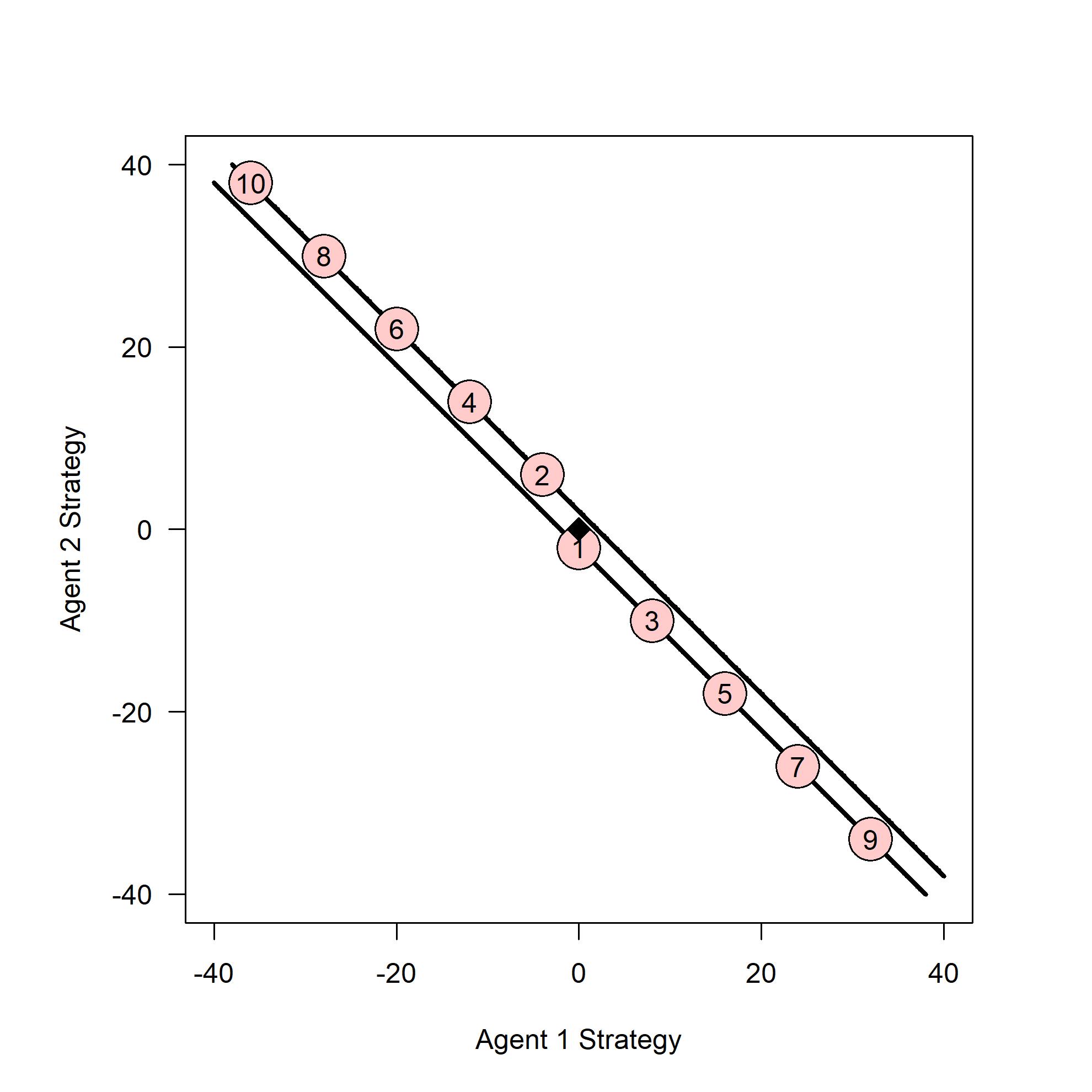
Proof.
Let , , and . Since , Theorem 4.11 does not imply and we cannot immediately claim the strategies will remain bounded. Using induction, we will show . The result trivially holds for .
By the inductive hypothesis, . Therefore
Similarly for agent 2,
Thus, agent 1’s strategy over time is the diverging sequence . ∎
4.6 Time-Average Convergence to Nash in Positive-Negative Definite Games

In this section, we show that the time-average of the strategies converge to the set of Nash equilibria at rate as depicted in Figure 6. We measure the distance to the set of Nash equilibria by . This is a standard measure since is a Nash equilibrium if and only if .
Theorem 4.11.
Suppose and commute with and respectively and when updating both agents’ strategies with Algorithm 2AltGD in (Positive-Negative Definite Game). Then agent 2’s strategy has time-average convergence to the set of Nash equilibria. Formally, there exists a constant such that for all , . Symmetrically, agent 1’s strategy also has time-average convergence to the set of Nash equilibria.
Perhaps surprisingly, we do not use the regret property to prove time-average convergence. Rather, time-average convergence follows immediately from the compact level sets of the energy function (Theorem 4.8).
Proof of Theorem 4.11.
By Theorem 4.8, belongs to a compact set and there exists a such that for each iteration . Recall that . Thus, completing the claim for agent 2.
The result for agent 1 follows identically using . ∎
We remark that the constant can be computed directly using the bound in Theorem 4.8. Once again, the bound on the learning rates is tight.
Proposition 4.12.
If the learning rates are too large when both agents use Algorithm 2AltGD in (Positive-Negative Definite Game), then time-average of the strategies may fail to converge – even if .
Proof.
In Proposition 4.10, we showed that for , , and that . Therefore, agent 1’s time-average strategy alternates between and on even and odd iterations thereby completing the proof. ∎
5 An Algorithm for Multiagent Systems
In this section, we extend our previous results to the multiagent system.
| (Network Game) |
Perhaps the most natural way to extend alternating gradient descent is to have agents iteratively take turns in a round-robin, i.e., agent 1 updates, then agent 2, and so on. However, in Section 5.1, we show this idea fails miserably – regret can grow linearly. The secret to the success of alternating gradient descent (Algorithm 2AltGD), doesn’t actually have anything to do with the perceived fairness of having agents take turns.
Instead, in Section 5.2 we extend the results for alternating gradient descent by understanding it as an approximation of a Hamiltonian system, a well-understood physical system. Specifically, alternating gradient descent naturally arises when approximating this continuous-time system using a symplectic integrator – specifically Verlet integration. In Section 5.3, we reduce the multiagent game to a 2-agent game through the use of two meta-agents and in Section 5.4, we extend the regret and conservation guarantees of Sections 3.1-3.4 to the multiagent case. Finally, in Section 5.5, we provide time-average convergence guarantees for positive-negative definite multiagent games.
5.1 Gradient Descent in a Round Robin
First, we consider a “fair” implementation of gradient descent where agents take turns updating and show that the algorithm can have linear regret.
Remark 5.1.
Proposition 5.2.
If agents take turns using gradient descent in a multiagent setting (Algorithm RoundGD), then an agent’s regret can grow linearly.
Proof.
Consider the simple 2-agent zero-sum game with and with initial strategies . Suppose both agents update according to Algorithm 2AltGD with learning rate . The agents strategies will cycle every 6 iterations (12 updates) as shown in Figure 7. As such, will gain 0 utility from any 6 consecutive iterations – from when agent 1 updates and from when agent 2 updates.
Now consider the addition of -dummy agents where for all and . Further suppose that all agents update according to Algorithm RoundGD, i.e., agent 1 updates, then agent 2, and so on. When agent updates, no agents will change their strategies since their payoff matrices are all zero. As a result, in the space of the first two agents, for each update spent at a red circle in Figure 7 there will be updates at the following blue square. Therefore every 6 round-robins (every cycle) will contribute to agent 1’s cumulative utility implying agent 1’s regret with respect to is . ∎
5.2 Designing a Multiagent Algorithm Based on Physics
As demonstrated by Proposition 5.2, the reason Algorithm 2AltGD works isn’t because it makes agents take turns in a seemingly fair fashion. Rather, Algorithm 2AltGD works because it is the result of a deep understanding of the physical system that drives gradient descent. By [6], the continuous-time version of 2-agent gradient descent is a Hamiltonian system (e.g., Earth-moon system) where agent 1 corresponds to “position” and agent 2 corresponds to “momentum”. The continuous-time variant has nice optimality and stability guarantees: time-average regret and recurrence in zero-sum games [21]. Algorithm 2AltGD is obtained by applying Verlet integration [3], an integration technique well-suited for approximating Hamiltonian dynamics [17], to the underlying Hamiltonian system.
Verlet integration corresponds to simply alternating between updating “position” and “momentum” in the underlying system. However, in the multiagent case, it is unclear which agents correspond to position and momentum respectively. Like [6], which shows the continuous-time system is Hamiltonian, we resolve this issue by allowing agents to be both position and momentum. However, instead of double-counting each agent as in [6], we instead duplicate each agent and build a game between the original and duplicated agents. Specifically, we allow the original agent control the strategy while their doppelganger controls strategy resulting in the following game.
| (Network Game with Duplicated Agents) | |||
Remark 5.3.
If the strategies and learning rates are initialized so that and , and if line 7 of Algorithm AltGD is replaced with (the original and duplicate agents update simultaneously) then in each iteration and the algorithm reduces to the standard version of gradient descent where the original agents simultaneously update with respect to the original agents’ previously played strategies (Algorithm SimGD).
Since no duplicate agent actually exists in many economic settings, Algorithm AltGD should primarily be used when interested in aggregate behavior, i.e., . Such applications are fairly standard in GANs and in other simulated environments such as bargaining and resource allocation problems that seeks a Nash equilibrium without agents directly sharing their payoff matrices, e.g., [25].
5.3 Reducing the Multiagent System to a 2-Agent Game
By introducing two meta-agents to control the original and duplicated agents, it is possible to express (Network Game) and Algorithm AltGD as 2-Agent Game and Algorithm 2AltGD respectively. Formally, we consider the following meta-game:
| (Meta-Game) | |||
where , and
In Theorem 5.4, we show the sets of Nash equilibria for (Meta-Game) and (Network Game) are equivalent. Moreover, in Theorem 5.5, we show that the Algorithms 2AltGD and AltGD result in the same updates for their respective games. As such, most of our results for 2-agent systems readily extend to the multiagent setting.
This reduction emphasizes the importance of allowing Algorithm 2AltGD to run with an arbitrary vector of learning rates. In the multiagent system, agents individually select their learning rates and therefore do not necessarily use the same learning rates. When applying Algorithm 2AltGD to (Meta-Game), the meta-agents will have different learning rates associated with each agent. Notably, our generalization still allows an individual to use different learning rates for different strategies, even in the multiagent setting. However, just like the 2-agent setting, we see no algorithmic benefit for a single agent to use a vector of learning rates.
Theorem 5.4.
The strategies are a Nash equilibrium for (Meta-Game) if and only if and are both Nash equilibria (possibly the same) for (Network Game).
Proof.
First, let be a Nash equilibrium of (Meta-Game). Then ; otherwise, meta-agent 1 could increase their utility by by updating their strategy to . Therefore, by definition of and , for each . It then holds that is a best response to (all strategies but agent ) in (Network Game) since for all . This holds for each agent and therefore i a Nash equilibrium for (Network Game). The argument for follow identically.
Next, let be a Nash equilibrium of (Network Game). Then for each since otherwise agent could increase their utility by with the strategy . As such, and is a Nash equilibrium of (Meta-Game). The argument holds identically for . ∎
Theorem 5.5.
Suppose is obtained by updating (Network Game) with Algorithm AltGD using learning rates and and initial strategies . Further, suppose is obtained by updating (Meta-Game) with Algorithm 2AltGD with learning rates and and initial strategy . Then for all .
Theorem 5.5 holds trivially by induction since the optimization problem is separable with respect to each agent.
5.4 Regret and Conservation in Multiagent Games
We show that Theorems 3.2 (regret) and 3.7 (volume conservation) both extend to this setting. We remark that Theorem 3.6 (self-actualization) also extends, however, as discussed in Section 5.2, Algorithm AltGD is best used in settings where only aggregate information () is of interest.
Theorem 5.6 ( Time-Average Regret).
If agent updates their strategies with Algorithm AltGD in (Network Game with Duplicated Agents) with an arbitrary vector of fixed learning rates , then their time-average regret with respect to an arbitrary fixed strategy in iteration is , regardless of how their opponents update.
Theorem 5.7 (Volume Conservation).
Algorithm 2AltGD in (Network Game with Duplicated Agents) is volume preserving for any measurable set of initial conditions.
Theorem 5.7 follow immediately by Theorem 3.7 after reducing (Network Game) to (Meta-Game). Theorem 5.6 almost follows similarly; certainly if all agents use Algorithm AltGD, then the corresponding meta-agent has time-average regret. Moreover, since is separable with respect to each individual agent’s strategy , each agent also obtains time-average regret. However, Theorem 5.6 only requires that agent 1 uses the update rule in Algorithm AltGD. To see that agent 1 still obtains time-average regret regardless of other agents, we consider the meta-game played between and the meta-agent where the meta-agent is using the same updates as in the original (Network Game).
Proof of Theorem 5.6.
Consider the following two-agent game:
| (Meta-Game for Agent ) | |||
where is the rows of corresponding to agent ’s payoff matrices against other agents and where is the columns of corresponding to other agents’ payoffs against agent .
Let be the updates obtained in (Network Game) where the original agent uses alternating gradient descent and let for all . This selection implies since and are updated with gradient descent with the same history of opponent play. Thus agent ’s utility and regret are the same in both (Network Game) and (Meta-Game for Agent i ). By Theorem 5.6, agent has time-average regret in (Meta-Game for Agent i ) and therefore also has time-average regret in (Network Game). ∎
5.5 Multiagent Positive-Negative Definite Games
Similar to Section 4, we introduce a Network Positive-Negative Definite Game and show that Algorithm AltGD conserves energy and achieves O(1/T) time-average convergence to the set of Nash equilibria.
| (Network Positive-Negative Definite Game) |
where .
Similarly, a Network Positive-Positive Definite Game is
| (Network Positive-Positive Definite Game) |
where .
Let
Then the multi-agent network positive-negative definite game can be reduced to a two-agent positive negative definite game with payoff matrices and ( for the positive-positive definite game). Thus the invariant energy functions from Section 4 immediately extend to the network setting.
Theorem 5.8 (Invariant Energy for (Network Positive-Negative Definite Game)).
Suppose and commute with and respectively. Then the perturbed energy is invariant when agents play (Network Positive-Negative Definite Game) and update their strategies with Algorithm AltGD.
Note that if commutes with then commutes with since both matrices are block diagonal and therefore any theorems that require that and commute hold in most standard applications of online optimization.
Theorem 5.9 (Invariant Energy for (Network Positive-Negative Definite Game)).
Suppose and commute with and respectively. Then the perturbed energy is invariant when agents play (Network Positive-Positive Definite Game) and update their strategies with Algorithm AltGD.
Moreover, following directly from Theorems 4.7, 4.8, and 4.11, Algorithm AltGD, is Poincaré recurrent, has bounded orbits, and converges to the set of Nash equilibria at rate O(1/T) in (Network Positive-Negative Definite Game).
Theorem 5.10 (Recurrence, Bounded Orbits, and Convergence).
Suppose and commute with and respectively and when updating both agents’ strategies with Algorithm AltGD in (Network Positive-Negative Definite Game). Then
- 1.
(Recurrence): for almost every initial condition , there exists an increasing sequence of iterations such that .
- 2.
(Bounded Orbits): agent strategies are bounded. Specifically,
- 3.
(Convergence): each agent has time-average convergence to the set of Nash equilibria.
6 Games with Additional Linear Payouts and Games Using Probability Vectors
We briefly remark that our results extend to the setting
| (Network Game with Additional Linear Payouts) |
A Nash equilibrium of this game satisfies for each agent . We can reduce this game to (Network Game) simply by expressing relative to for each agent . Formally, let (in our setting, is affine and therefore ). Thus, (Network Game with Additional Linear Payouts) is equivalent to
From agent ’s perspective, is constant. Thus, all maximizers of the previous expression also maximize
Thus, a game with additional linear payouts can always be expressed as a game without additional linear payouts after shifting the strategy space. Moreover, the constant plays no role for online optimization methods that rely on gradients of the utility function, e.g., gradient descent. Thus, the behavior of gradient descent will remain unchanged and all previous results extend to (Network Game with Additional Linear Payouts).
This reduction gives some ideas on how to extend these results when is the set of probability vectors, i.e., . After performing the substitution for each agent , a network game using probability vectors reduces to (Network Game with Additional Linear Payouts) where is a compact, full-dimensional space. As long as the strategies remain in the interior when using Algorithm AltGD, the optimality guarantees will extend as well. Regrettably, the space is not affine and the energy function may change when the strategies intersect with boundary and more theory needs to be developed to understand this setting.
7 Experiments: Performance Relative to Optimistic Variants
In practice, optimistic variants of follow-the-regularized-leader algorithms, e.g., optimistic gradient descent (Algorithm OptGD below), are often used due to their time-average convergence to the set of Nash equilibria in zero-sum games. With the results of Sections 4 and 5, Algorithm AltGD provides another option for fast convergence.
To obtain this guarantee, Algorithm OptGD requires the learning rate [23] while our approach, Algorithm AltGD, only requires . By Theorems 3.4 and 3.5, larger learning rates lead to stronger optimization guarantees. As such, we hypothesize that by using larger learning rates, Algorithm AltGD can outperform OptGD.
In this section, we perform experiments to support this hypothesis and find that with 97.5% confidence, Algorithm AltGD, on average, results in time-averaged strategies that are 2.585 times closer to the set of Nash equilibria than Algorithm OptGD. We also compare Algorithm AltGD to an optimized version of Algorithm OptGD that uses additional memory to avoid matrix products. With 97.5% confidence, Algorithm AltGD, on average, results in time-averaged strategies that are 1.742 times faster to the set of Nash equilibria than the optimized version of Algorithm OptGD.
We remark that our approach, Algorithm AltGD has a distinct advantage over Algorithm OptGD as we guarantee time-average convergence in a generalization of zero-sum games – a result not known for Algorithm OptGD. However, we conjecture that many results currently in the literature extend to Network Positive-Negative Definite Games using the techniques we introduced in Section 4.
7.1 Description of Experiments
We compare the performance of alternating and optimistic gradient descent with agents where each agent has the same number of strategies (). We compare the performance of each algorithm across 30 games where is selected uniformly at random from for and where for (a zero-sum game) and perform statistical analysis after pairing the samples for each game in order to reduce the variance in the statistical estimates. For both algorithms, we select the learning rate to be as large as possible while still ensuring time-average convergence guarantees for any randomly selected set of payoff matrices. Specifically, we use the learning rate for alternating gradient descent and for optimistic gradient descent. As discussed in Section 7.2, this selection normalizes the learning rates of the two algorithms.
In our experiments, we also use an optimized version of optimistic gradient descent that uses more memory in exchange for computing fewer matrix products (Algorithm ¯ Opt GD below) and compare our method to both the standard and optimized implementations of optimistic gradient descent. Specifically, for a single game and initial condition, we run each of the three algorithms for 30 seconds and measure the distance to the Nash equilibrium with respect to the dual space – we measure where is the combined payoff matrix introduced in Section 5.3. As discussed in Section 4.6, if only if is a Nash equilibrium and measures the distance to the Nash equilibrium in a dual space.
Denote , and as the distance after 30 seconds of running Algorithms OptGD, ¯ Opt GD, and AltGD respectively. Since each instance of , and are generated from the same game and initial condition and are also run in sequence, we can pair the results of the individual instances to get an estimate on relative performances and .
All experiments were conducted in version 4.02 of the R-statistical software on Windows 10 using an i7-10700 processor (2.9GHz) with 32GB of RAM. To control for variability caused by computer processing, we generate a single game and run all three algorithms on the game prior to generating the next game. The source code and spreadsheet of results for the experiments can be downloaded at www.jamespbailey.com/1OverTConvergence.
7.2 Selection of Learning Rates
In our experiments, we use a single scalar learning rate for all agents. To guarantee optimistic gradient descent has time-average convergence to the set of Nash equilibria, is required to be at most [23]. However, as shown in Theorem 4.11, alternating gradient descent only requires . As such, in our experiments, we always select the learning rate for alternating gradient descent to be four times larger than the learning rate for optimistic gradient descent, i.e., . As shown in Theorems 3.4 and 3.5, larger learning suggest better performance for alternating gradient descent and if is a valid learning rate for optimistic gradient descent, then is a valid learning rate for alternating gradient descent.
We remark that this selection normalizes the values of the learning rates; we are forcing both algorithms to operate near the boundary for optimal performance, i.e., and . As shown in Lemma B.1 in the Appendix, and therefore we select learning rates and for alternating and optimistic gradient descent respectively. As suggested by Propositions 4.10 and 4.12, will not perform well when . However, the probability that is since the elements of are generated uniformly at random.
7.3 Results of Experiments
In all 270 generated instances, our method (alternating gradient descent) outperformed both implementations of optimistic gradient descent. Specifically, alternating gradient resulted in strategies that were approximately 2.628 and 1.772 times closer to the set of Nash equilibria than the standard and optimized implementation of optimistic gradient descent respectively. Moreover, across all selections of agents and strategies, we are 97.5% confident that, on average, alternating gradient descent will result in strategies that are 2.585 and 1.743 times closer to the set of Nash equilibrium after 30 seconds than the standard and optimized implementation of optimistic gradient descent respectively. Thus, alternating gradient descent performs significantly better than both implementations of optimistic gradient descent.
The relative performance of alternating gradient descent for agents and strategies can be viewed in Tables 1 and 2. For example, in 20 agent, 20 strategy games, we are 97.5% confident that alternating gradient descent, on average, alternating gradient descent will result in strategies that are 2.5902 and 1.8040 times closer to the set of Nash equilibrium than the standard and optimized implementation of optimistic gradient descent respectively.
7.4 Importance of Large Learning Rates
Finally, we test the importance of using larger learning rates; a key feature of alternating gradient descent is that it enables learning rates four times larger than optimistic gradient descent. As suggested by Theorems 3.4 and 3.5 and shown in Table 3, larger learning rates are vital for Algorithm AltGD’s superior performance.
| (0.6376,0.6934) | (1.2168,1.3325) | (2.5003,2.7186) | |
| (0.4236,0.4706) | (0.7906,0.8725) | (1.6482,1.7849) |
8 Conclusion
In this paper, we have proven that alternating gradient descent achieves time-average convergence to the set of Nash equilibria in a generalization of network zero-sum games. Further, we have experimentally shown with 97.5% confidence that, on average, alternating gradient results in time-averaged strategies that are 2.585 times closer to the set of Nash equilibria than optimistic gradient descent. In addition to providing a faster algorithm for a more general set of games, this paper also demonstrates the potential power of carefully constructing close approximations of continuous-time learning dynamics.
References
- [1] Jacob Abernethy, Kevin A Lai, and Andre Wibisono. Last-iterate convergence rates for min-max optimization: Convergence of hamiltonian gradient descent and consensus optimization. In Algorithmic Learning Theory, pages 3–47. PMLR, 2021.
- [2] Bharat Adsul, Jugal Garg, Ruta Mehta, Milind Sohoni, and Bernhard Von Stengel. Fast algorithms for rank-1 bimatrix games. Operations Research, 69(2):613–631, 2021.
- [3] James P Bailey, Gauthier Gidel, and Georgios Piliouras. Finite regret and cycles with fixed step-size via alternating gradient descent-ascent. In Conference on Learning Theory, pages 391–407. PMLR, 2020.
- [4] James P. Bailey and Georgios Piliouras. Multiplicative weights update in zero-sum games. In Proceedings of the 2018 ACM Conference on Economics and Computation, EC ’18, page 321–338, New York, NY, USA, 2018. Association for Computing Machinery.
- [5] James P. Bailey and Georgios Piliouras. Fast and furious learning in zero-sum games: Vanishing regret with non-vanishing step sizes. In Advances in Neural Information Processing Systems 32, pages 12977–12987. Curran Associates, Inc., 2019.
- [6] James P. Bailey and Georgios Piliouras. Multi-agent learning in network zero-sum games is a hamiltonian system. In Edith Elkind, Manuela Veloso, Noa Agmon, and Matthew E. Taylor, editors, Proceedings of the 18th International Conference on Autonomous Agents and MultiAgent Systems, AAMAS ’19, Montreal, QC, Canada, May 13-17, 2019, pages 233–241. International Foundation for Autonomous Agents and Multiagent Systems, 2019.
- [7] Maria-Florina Balcan, GATECH EDU, Florin Constantin, HARVARD EDU, Ruta Mehta, and IITB AC. The weighted majority algorithm does not converge in nearly zero-sum games. Rn, 1:S2, 2012.
- [8] Luis Barreira. Poincare recurrence: old and new. In XIVth International Congress on Mathematical Physics. World Scientific., pages 415–422, 2006.
- [9] Yang Cai, Ozan Candogan, Constantinos Daskalakis, and Christos Papadimitriou. Zero-sum polymatrix games: A generalization of minmax. Mathematics of Operations Research, 41(2):648–655, 2016.
- [10] Nicolo Cesa-Bianchi and Gábor Lugosi. Prediction, learning, and games. Cambridge university press, 2006.
- [11] Yun Kuen Cheung and Georgios Piliouras. Chaos, extremism and optimism: Volume analysis of learning in games, 2020.
- [12] C Daskalakis and Ioannis Panageas. Last-iterate convergence: Zero-sum games and constrained min-max optimization. In 10th Innovations in Theoretical Computer Science (ITCS) conference, ITCS 2019, 2019.
- [13] Constantinos Daskalakis, Maxwell Fishelson, and Noah Golowich. Near-optimal no-regret learning in general games, 2021.
- [14] Simon S Du, Jianshu Chen, Lihong Li, Lin Xiao, and Dengyong Zhou. Stochastic variance reduction methods for policy evaluation. In International Conference on Machine Learning, pages 1049–1058. PMLR, 2017.
- [15] Noah Golowich, Sarath Pattathil, Constantinos Daskalakis, and Asuman Ozdaglar. Last iterate is slower than averaged iterate in smooth convex-concave saddle point problems. In Conference on Learning Theory, pages 1758–1784. PMLR, 2020.
- [16] Ian J. Goodfellow, Jean Pouget-Abadie, Mehdi Mirza, Bing Xu, David Warde-Farley, Sherjil Ozair, Aaron Courville, and Yoshua Bengio. Generative adversarial networks, 2014.
- [17] Ernst Hairer. Long-time Energy Conservation, page 162–180. London Mathematical Society Lecture Note Series. Cambridge University Press, 2006.
- [18] Ernst Hairer, Marlis Hochbruck, Arieh Iserles, and Christian Lubich. Geometric numerical integration. Oberwolfach Reports, 3(1):805–882, 2006.
- [19] Ehsan Asadi Kangarshahi, Ya-Ping Hsieh, Mehmet Fatih Sahin, and Volkan Cevher. Let’s be honest: An optimal no-regret framework for zero-sum games. In International Conference on Machine Learning, pages 2488–2496. PMLR, 2018.
- [20] Ravi Kannan and Thorsten Theobald. Games of fixed rank: A hierarchy of bimatrix games. Economic Theory, 42(1):157–173, 2010.
- [21] Panayotis Mertikopoulos, Christos Papadimitriou, and Georgios Piliouras. Cycles in adversarial regularized learning. In Proceedings of the Twenty-Ninth Annual ACM-SIAM Symposium on Discrete Algorithms, SODA ’18, page 2703–2717, USA, 2018. Society for Industrial and Applied Mathematics.
- [22] Panayotis Mertikopoulos and William H Sandholm. Learning in games via reinforcement and regularization. Mathematics of Operations Research, 41(4):1297–1324, 2016.
- [23] Aryan Mokhtari, Asuman E Ozdaglar, and Sarath Pattathil. Convergence rate of O(1/k) for optimistic gradient and extragradient methods in smooth convex-concave saddle point problems. SIAM Journal on Optimization, 30(4):3230–3251, 2020.
- [24] Henri Poincaré. Sur le problème des trois corps et les équations de la dynamique. Acta mathematica, 13(1):A3–A270, 1890.
- [25] S. Pu, J. J. Escudero-Garzas, A. Garcia, and S. Shahrampour. An online mechanism for resource allocation in networks. IEEE Transactions on Control of Network Systems, pages 1–1, 2020.
- [26] Walter Rudin. Real and complex analysis (mcgraw-hill international editions: Mathematics series). 1987.
- [27] Chen-Yu Wei, Chung-Wei Lee, Mengxiao Zhang, and Haipeng Luo. Linear last-iterate convergence in constrained saddle-point optimization. arXiv preprint arXiv:2006.09517, 2020.
Appendix A Proof of Proposition 3.9
See 3.9
Proof.
With the selection of learning rates and the payoff matrix , one iteration of Algorithm 2AltGD maps the point . Since the mapping is linear and is convex with a finite number of extreme points, will also be convex with a finite number of extreme points. Moreover, the extreme points of can be determined directly from the extreme points of . Let denote the extreme points of . We begin by claiming that where is the th number in the Fibonacci sequence. The sequence is defined by with .
We proceed induction and consider . Extending the sequence backwards, and . Thus, for , completing the base case. Next, by the inductive hypothesis, . As stated before, we compute directly from using the map : First,
Following identically, . Next,
Similarly, . Thus, as claimed.
The diameter of is then given by the distance between and since is increasing for . This distance is . It is well-known that where is the golden ratio. Thus,
and the diameter grows exponentially.
Finally, the volume of is 4. By Theorem 3.7, Volume is invariant and therefore the volume of is also 4 thereby completing the proof. ∎
Appendix B Bounding for Experiments
Lemma B.1.
Let for all and for and let . Let be the combined payoff matrix as defined in Section 5.3. Then . Further, there exists an instance such that .
The first part of the proof consists of showing that where is a coordination game with . We then show that the largest eigenvalue of is implying . The second part of the proof simply consists of giving an and such that .
Proof.
Let be an arbitrary matrix. We first show that if is such that then . Let be such that as in the definition of . Then,
Next, let be a vector of 1’s and let for all (a matrix of 1’s) and let . This corresponds to a coordination game where the payout for every pair of pure strategies is 1. By selection, when is generated between and and therefore, by the previous claim, .
It is well-known that the spectral norm and Euclidean norms are equivalent, i.e., where is the largest eigenvalue for . Let and be any eigenvalue/eigenvector pair for . We write the components of the eigenvector as in order to freely move between the notations and . We also use to denote the portion of the eigenvector that multiplies by in the definition of an eigenpair. Since and are an eigenpair,
The term is a vector of constants and there exists a such that . Continuing from above, this implies
Further, we may select and so that which implies there exists an such that and . Selecting such an implies
where the last inequality follows since is a concave function over a convex, symmetric domain and therefore has the symmetric maximizer for all . Thus, . We remark that that this bound for is tight – it is straightforward to verify that and are an eigenpair. This completes the first part of the proof since .
To show , let for and let for . As such, is block diagonal matrix with 0’s on the block diagonal, positive 1’s above the diagonal, and negative 1’s below the diagonal. Then
∎