Asymptotic Distributions for Likelihood Ratio
Tests
for the Equality of Covariance Matrices
Wenchuan Guoa, Yongcheng Qib
aBiometrics & Data Sciences, Bristol Myers Squibb, 3551 Lawrenceville Princeton, Lawrence Township, NJ 08543, USA.
bDepartment of Mathematics and Statistics, University of Minnesota Duluth, 1117 University Drive, Duluth, MN 55812, USA.
Abstract. Consider independent random samples from -dimensional multivariate normal distributions. We are interested in the limiting distribution of the log-likelihood ratio test statistics for testing for the equality of covariance matrices. It is well known from classical multivariate statistics that the limit is a chi-square distribution when and are fixed integers. Jiang and Yang [13] and Jiang and Qi [12] have obtained the central limit theorem for the log-likelihood ratio test statistics when the dimensionality goes to infinity with the sample sizes. In this paper, we derive the central limit theorem when either or goes to infinity. We also propose adjusted test statistics which can be well approximated by chi-squared distributions regardless of values for and . Furthermore, we present numerical simulation results to evaluate the performance of our adjusted test statistics and the log-likelihood ratio statistics based on classical chi-square approximation and the normal approximation.
Keywords: Likelihood ratio test, central limit theorem, multivariate normal distribution, multivariate Gamma function.
1 Introduction
High-dimensional data are increasingly common in many applications of statistics, encountered particularly in biological, meteorological, and financial studies. If we have observations from a -dimensional population, it is natural to set up an data matrix. The analysis of such matrices includes hypothesis testing, interval estimation and modeling, and is elaborated in many classical textbooks of multivariate analysis such as Anderson [2], Muirhead [16], and Eaton [9]. In these books, the properties of these tests, estimations or models are based on the assumption that the data dimensionality is a fixed constant or is negligible compared with the sample size . However, due to the explosive development and improvement of computing power and data collection methods, the data dimension is often high. The traditional assumption of small large is no longer valid because the dimensionality can be proportionally large compared with the sample size . Some recent results in this situation have been found in Bai et al. [3], Ledoit and Wolf [14], Jiang et al. [11], Jiang and Yang [13], Jiang and Qi [12], Dette and Dörnemann [8], and references therein.
Given that independent samples are observed and each of them is from a -dimensional multivariate normal distribution, we are interested in testing the equality of covariance matrices of multivariate normal distributions under the assumption that either , or , or both. The results in this direction can be very useful when one considers multivariate analysis of variance problems for high dimensional data that are resulted from a large number of treatments.
We denote as the multivariate normal distribution with dimensionality , where is the mean vector and is the covariance matrix. Assume is an integer. Let }, be independent random samples from , where the mean vectors and covariance matrices are unknown. Consider the following hypothesis test:
| (1.1) |
Define
and
The likelihood ratio test for (1.1), derived by Wilks [22], is as follows:
The details can be found in Section 8.2.2 of Muirhead [16]. The test statistic is non-degenerate only if every is of full rank, which means that is required for all , i.e, . However, the drawback of this likelihood-ratio test is that it is biased when the sample sizes are not all equal, which means that the probability of rejecting in (1.1) when is true can be larger than the probability of rejecting with is false. This phenomenon was first noticed by Brown [6] with . In what follows, we use instead the following modified likelihood ratio test statistic suggested by Bartlett [4]:
| (1.2) |
is derived by substituting the sample size by the degree of freedom and sum of by . It is proved by Sugiura and Nagao [21] that this modified likelihood ratio test is unbiased when . A generalization to general integer is made in Perlman [17].
Assume and are fixed integers. Under the null hypothesis in (1.1), Box [5] proved that has a chi-square limit
| (1.3) |
as , where
| (1.4) |
and
Note that converges to as . The classic theory for likelihood ratio test statistics states that . The correction factor is introduced in (1.3) for a better chi-square approximation rate.
The likelihood ratio test of size based on the asymptotic distribution of is to reject (1.1) when the sample is falling on the region
| (1.5) |
where is the -level upper quantile of distribution. The details can be found in Muirhead [16], p.308.
In recent studies, the assumption on the fixed dimensionality is relaxed to change with the sample size so that the ratio converges to a constant between 0 and 1, i.e.,
| (1.6) |
For instance, using the Random Matrix Theory method, the correction to the traditional likelihood ratio test for testing the equality of two covariance matrices is given in Bai et al. [3] as
where the two sample covariance matrices are denoted as and , and a central limit theorem is established for under assumption (1.6). An extension to case is also considered in Jiang, Jiang and Yang [11]. Furthermore, for likelihood ratio test for the equality of covariance matrices, Jiang and Yang [13] and Jiang and Qi [12] have obtained the following central limit theorem (CLT)
| (1.7) |
where and are asymptotic mean and standard deviation as the functions of and . In their work, is a fixed integer, the dimensionality can be proportionally large to the sample size or much smaller than , that is, and for .
The central limit theorem (1.7) can also be true when both and change with the sample sizes. Guo [10] and Dette and Dörnemann [8] establish the asymptotic normality under very restrictive conditions on both and . See Remark 3 in Section 2 for more details.
The likelihood ratio statistic cannot be applied to the test of the homogeneity of several covariance matrices if the dimensionality is larger than some of the sample sizes since the corresponding sample covariance matrices are singular. To overcome this problem, Schott [19], Srivastava and Yanagihara [20] propose two test statistics based on trace of sample covariance matrices. Subsequent papers such as Li and Chen [15], Cai, Liu and Xia [7], Yang and Pan [23], and Zheng et al. [24] have developed various test statistics which can be also applied to non-normal populations.
Our objective in this paper is to investigate the limiting distribution of the log-likelihood ratio test statistic for the multivariate normal distributions under the minimal conditions. We have pointed out that the likelihood ratio test exits only if . In this paper, we assume that both and can change with sample sizes, , and tends to infinity. We will show in Theorem 2.1 that , after properly normalized, converges in distribution to the standard normal distribution if . Without imposing this additional condition, we propose an adjusted log-likelihood ratio test statistic (ALRT) in (2.7) in Section 2 and prove in Theorem 2.2 that the ALRT statistic is approximately distributed a chi-square with degrees of freedom. Neither nor shares this property when or are too large.
The rest of the paper is organized as follows. In Section 2, we give the main results in the paper, including the CLT for and chi-square approximation to the ALRT statistics and some discussions; In Section 3, we carry out a simulation study to compare the performance of based on the classical chi-square approximation, the normal approximation and the ALRT statistics based on the chi-square approximation. All proofs are provided in Section 4.
2 Main results
We first introduce some notations. Let denote the gamma function given by
Define the digamma function by
| (2.1) |
Define
| (2.2) |
is nonnegative in .
Throughout this paper, we write and assume that the minimal sample size goes to infinity. Furthermore, both the dimensionality parameter and number of the populations can diverge. For this reason, we write and to indicate that both parameters may change with the sample sizes.
Define
| (2.3) | |||||
and
| (2.4) |
Based on the Theorem 2.1, the rejection region of the test (1.1) at level is
| (2.6) |
where is level critical value of the standard normal distribution.
The chi-square appropriation in (1.3) and the central limit theorem in Theorem 2.1 exhibit two different types of limiting distributions for inference. As our simulation study in Section 3 indicates, when is small, the chi-square approximation (1.3) works very well; while is large, the normal approximation prevails. In practice, one needs to decide which approximation should be used. The two theoretical results don’t clearly suggest when to use the normal approximation and when to use the chi-square approximation. It is desirable if we are able to construct a test statistic which is a linear function of with a unified asymptotic distribution regardless of values of and . The chi-square distributions are better choices than the normal distribution for this purpose since is not asymptotically normal when both and are small. We note that the ratio of the mean and the variance of a chi-square distribution is . However, neither nor is well approximated by a chi-square distribution when is too large as the ratio of their asymptotic means and variances is not very close to in this case.
We propose the following adjusted log-likelihood ratio test (ALRT) statistic
| (2.7) |
where as given in (1.4), and are defined in (2.3) and (2.4), respectively. Note that the ALRT is essentially the LRT statistic since it is a linear function of the log-likelihood ratio test statistic, . This new test statistic achieves an asymptotic mean and an asymptotic variance . We have the following theorem regarding the chi-square approximation of statistic.
Theorem 2.2.
Assume and are two sequences of integers, and . Then we have under in (1.1) that
| (2.8) |
Based on Theorem 2.2, the rejection region of the test (1.1) at level is
| (2.9) |
where is the -level critical value of a chi-square distribution with degrees of freedom.
Under some restrictive conditions, we can avoid using the digamma function when we approach the mean of . We have the following theorem.
Theorem 2.3.
Remark 1. In both Theorems 2.1 and 2.2, we assume and as . The first condition ensures the likelihood ratio test statistics exist and the second condition guarantees that the minimal sample size goes to infinity so that the asymptotic properties of can be investigated. Both conditions are necessary and cannot be weakened. Theorem 2.1 shows that a necessary and sufficient condition for the central limit theorems is , which is equivalent to , where . If is bounded or fixed, the distribution of is well approximated by distribution. More generally, Theorem 2.2 ensures that the ALRT statistic, as defined in (2.7), is well approximately by .
Remark 2. In both
Theorems 2.1 and 2.2, the digamma function
as defined in (2.1) is involved in the computation of the
asymptotic mean of via equation
(2.3). We notice that the digamma function is built in
software R and can be calculated using the digamma
function in R.
Remark 3. Assume the null hypothesis in (1.1) holds, , and . Our Theorem 2.1 indicates that is the necessary and sufficient for the central limit limit theorems of . In Guo [10], it is shown that
under additional conditions that , as , and there exists a constant such that for all large . Theorem 3 in Dette and Dörnemann [8] states that , after properly normalized, converges in distribution to the standard normal under a different set of additional assumptions that , , as , and there exists a constant such that for all large . Clearly, either in Guo [10] or Dette and Dörnemann [8], the following situations are not under consideration:
(a) ;
(b) .
Remark 4. As we have mentioned earlier, conditions and are necessary for discussion on the asymptotic distribution of . Theorem 2.2 indicates that the new test statistic can be approximated by chi-square distribution uniformly over and as . However, there is a transition from chi-square to the normal in the limiting distribution of .
3 Simulation study
In this section, we carry out some simulation studies to compare the performance for the likelihood ratio test statistics based on three different approximations, including the classic chi-square approach (1.3), the CLT approach (2.5) and ALRT approach (2.8). The corresponding rejection regions for a size test on (1.1) are given in equations (1.5), (2.6) and (2.9), respectively.
We compare the three test statistics as follows: a). We plot the histograms of the three statistics and see how well the histograms for each statistic fits its theoretical distribution under the null hypothesis of (1.1); b). We estimate the sizes (or type I errors) and determine which test statistic is more accurate; c). We estimate the power for each test statistic under some alternative hypotheses of (1.1).
For each combination of and with and , we set for . We generate random samples with sample sizes respectively from multivariate normal distributions with selected covariance matrices, and then we calculate three test statistics. Histograms, estimation of sizes and powers are based on replicates. In our histograms and tables for sizes and powers for three test statistics, we use “Chisq”, “CLT” and “ALRT” to denote the classic chi-square approximation (1.3), normal approximation (2.5), and adjusted chi-square approximation (2.8), respectively.
3.1 Histograms and empirical sizes
We generate random samples from multivariate normal distributions under the null hypothesis of (1.1). Denote the common variance matrix as which is a by matrix. Since the distribution function of doesn’t depend on the matrix , we can simply set as a by identity matrix.
For each combination of and , we plot the histograms for the three standardized test statistics, namely , , and . The histograms for these statistics are also compared with their approximate density functions – a chi-squared distribution with degrees of freedom, the standard normal distribution, and a chi-squared distribution with degrees of freedom, respectively, as established in (1.3), (2.5) and (2.8). See Figure 1 and Figures S2 and S3 in the supplement.
The histograms in Figure 1 and Figures S2 and S3 reveal the overall performance for the three test statistics. We can conclude that the classic chi-square approximation works well when is small and gets worse as increases, the normal approximation starts to get better as increases, and only the histograms for the adjusted test statistic fit the chi-squared curves in all cases.
The empirical sizes for all three tests at level are reported in Table 1. A good test in terms of the type I errors (or sizes) will have an actual size close to its nominal level . The adjusted test statistic outperforms over the other two test statistics since its sizes are close to in all cases. In particular, the classic chi-square approximation performs well only when is relatively small. When is large, the null hypothesis is rejected with a probability close to one.


| Conditions | Chisq | CLT | ALRT |
|---|---|---|---|
| 0.0501 | 0.0636 | 0.0529 | |
| 0.0575 | 0.0608 | 0.0569 | |
| 0.1861 | 0.0539 | 0.0521 | |
| 1.0000 | 0.0689 | 0.0678 | |
| 0.0511 | 0.0576 | 0.0529 | |
| 0.0639 | 0.0542 | 0.0530 | |
| 0.8135 | 0.0533 | 0.0529 | |
| 1.0000 | 0.0618 | 0.0614 | |
| 0.0490 | 0.0540 | 0.0505 | |
| 0.0755 | 0.0525 | 0.0519 | |
| 0.9937 | 0.0554 | 0.0551 | |
| 1.0000 | 0.0619 | 0.0618 |
3.2 Comparison of powers
The power of a test is the probability of rejecting when is false. For each combination of and , we take random samples, and the -th sample is from a multivariate normal distribution with mean vector 0 and covariance matrix for , where is a by identity matrix, and is a by matrix with all entries being equal to . Again, all sample sizes are the same with in the study. The powers for the three test statistics are estimated based on replicates, and they are reported in Table 2.
We first note that all three test statistics are linear combinations of , the corresponding rejection regions at level are of the same type as . The only difference is that the values of cutoff corresponding to the three approximations are different. That means the three rejections and , defined in (1.5), (2.6) and (2.9), respectively, are nested each other. A large rejection region has a larger size of test and a larger power as well. From Table 2, we can see that whenever any two test statistics have really close sizes, they have similar powers. When the classic chi-square approximation fails, that is, it produces a large size, it also yields a large power. However, its large power does not make any sense here. So we compare the normal approximation and the chi-square approximation based on the test statistic . We observe that both test statistics have comparable powers when the normal approximation achieves a reasonable size.
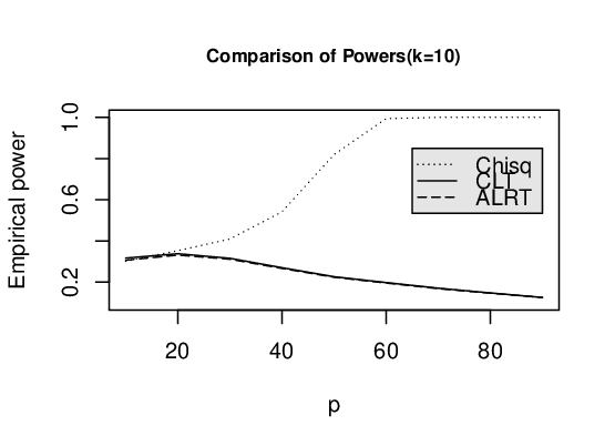
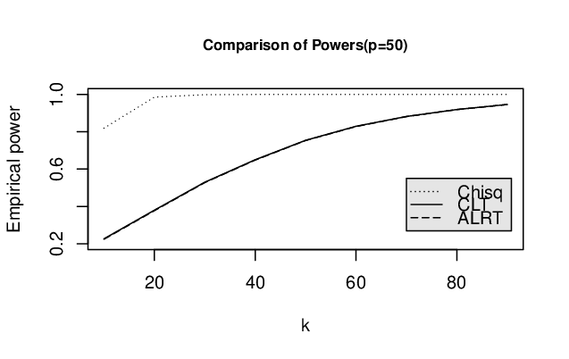
Finally, we will demonstrate how the powers of the three test statistics change with or while other variables remain constant. For illustration purpose, we set and when increases from to , and set and when increases from to . The covariance structures are the same as specified in the beginning of this subsection. The curves of the powers for the three test statistics are plotted in Figure 2. We see that the power of the classic chi-square statistic (Chisq) is much larger when is bigger, and this is the case for the two plots in the figure. Keep in mind that we have set in the second plot in Figure 2. This phenomenon happens since the classic chi-square approach results in a much larger type I error than the nominal level as in Table 1. Two other methods are very close in terms of power.
| Conditions | Chisq | CLT | ALRT |
|---|---|---|---|
| 0.0744 | 0.0958 | 0.0778 | |
| 0.1203 | 0.1260 | 0.1194 | |
| 0.3249 | 0.1233 | 0.1197 | |
| 1.0000 | 0.0987 | 0.0976 | |
| 0.5587 | 0.5809 | 0.5656 | |
| 0.7025 | 0.6728 | 0.6690 | |
| 0.9858 | 0.3798 | 0.3775 | |
| 1.0000 | 0.1478 | 0.1473 | |
| 0.9992 | 0.9992 | 0.9992 | |
| 0.9971 | 0.9951 | 0.9951 | |
| 1.0000 | 0.7544 | 0.7534 | |
| 1.0000 | 0.2284 | 0.2278 |
3.3 Concluding remark
In this paper, we study the limiting distribution of the likelihood ratio test statistics for testing equality of the covariance matrices from multivariate normal populations. We allow both and the dimensionality of the populations to change with the sample sizes. We establish the central limit theorem for the log-likelihood test when tends to infinity. Further, we propose an adjusted log likelihood test statistic and prove that the distribution of the new test statistic can be well approximated by a chi-squared distribution regardless of how and change with the sample sizes. This new test outperforms in terms of accuracy in type I error and has the comparable power as the classic chi-square approximation or the normal approximation when they are applicable.
4 Proofs
The standard notation to describe the limiting behavior of a function is denoted by big and small . Precisely, for two sequences of numbers and , as means that and as means that . The symbol stands for . For two functions and , we also use , and with the similar meaning as .
The multivariate gamma function, denoted by , is defined as
| (4.1) |
for complex numbers with Re, where is an integer. In our applications we only need to consider for real variable . We will put much effort in expand the function below.
The function defined in (2.2) is nonnegative in . It is easy to see that and . We have
By writing , we have , and
Now we define
| (4.2) |
We can conclude that
| (4.3) |
4.1 Some auxiliary lemmas
Lemma 4.1.
Proof. One can easily verify
| (4.4) |
and
| (4.5) |
Then it follows from equations (4.3), (4.4) and (4.5) that
as . This completes the proof.
Lemma 4.2.
As
| (4.6) |
and
| (4.7) |
Proof. Let be any sequence of integers satisfying Lemma 4.1. Since
and , we have
which converges to zero as according to Lemma 4.1. This proves (4.6)
(4.7) can be proved in the same manner and the details are omitted.
Lemma 4.3.
For any , there exist constants and such that
| (4.8) |
| (4.9) |
Proof. Without loss of generality, assume .
It follows from Formulas 6.3.18 and 6.4.12 in Abramowitz and Stegun [1] that
as . Therefore, there exist constant and such that (4.8) and (4.9) hold for with . It remains to show that (4.8) and (4.9) hold for . We show (4.8) only for illustration. Since the function is continuous in , we have . By setting , we have
Obviously, we also have
Lemma 4.4.
Define
and
| (4.10) |
Then we have
| (4.11) |
and there exists a constant such that
Lemma 4.5.
We have for any
| (4.12) |
Lemma 4.6.
As ,
| (4.13) |
| (4.14) |
| (4.15) |
| (4.16) |
and for any fixed
| (4.17) |
uniformly over as .
Recall the relation of and from (4.2) that for . Then we have
Let be any sequence of integers such that and as , From from Lemma 4.1 we have
and
which combined with (4.13) yields that (4.15) holds uniformly over as . It remains to show that (4.15) holds uniformly over as . In fact, by uisng Taylor’s expansion we have uniformly over
and
which imply
uniformly over as . In the las step we use that as and . This completes the proof of (4.15).
Lemma 4.7.
Proof. Without loss of generality, assume . Since and , we have
Also note that as . From (4.3), and . We have for all large
which implies (4.18).
Lemma 4.8.
Proof. Define
Then we have for any positive integers with
| (4.23) |
Since , we have from (4.20) that for all large and as .
From (4.23), (4.8), condition (4.21) and Lemma 4.7 we have
and
Hence we have
In view of (2.3), (4.23), and equations (4.14) and (4.13) in Lemma 4.6 we have
Moreover, under condition (4.21), we have
and
Then we conclude (4.22).
Let be any function defined over . For integers and with , define the function
| (4.24) |
We need this definition in the following proofs.
Lemma 4.9.
For any integers , define
where the function is defined in Lemma 4.4. Then
| (4.25) | |||||
and
| (4.26) | |||||
hold uniformly over , as and .
Proof. We will apply Taylor’s theorem to expand a smooth function , that is, that is, for any , there exists a constant between and such that
| (4.27) |
In our application here, we will assume , and .
We note that
| (4.28) |
when , .
From (4.11), (4.28), and Lemma 4.5 we have
and, thus from (4.17), (4.6), (4.2) and (4.3)
holds uniformly over , as and . Furthermore, in view of (4.11), (4.15) and (4.16) we have
uniformly over as . (4.25) can be easily obtained by combining all results above.
Review the definition of in Lemma 4.4 and the definition of in (4.24). Since , we have
By using (4.25) and the fact that
we conclude (4.26).
Lemma 4.10.
We have
uniformly over , as and .
For function defined in (4.10), we apply Taylor’s formula with remainder
| (4.30) |
where is a number between and . Using Lemma 4.4 we have for some
Summing up over on both sides of (4.30) yields
| (4.31) | |||||
uniformly over , as and . In the above estimation, we have used (4.17) from Lemma 4.6 and (4.7) from Lemma 4.2.
From (4.10), we have
Now by combining (4.29), (4.31), (4.26) and the above equations we have
uniformly over , as and . This completes the proof of the lemma.
Finally, we state the following lemma to express the moments of as a product of functions, which is available on page 302 in Muirhead [16].
4.2 Proofs of the main results
Proof of Theorem 2.1.
We first show the sufficiency, that is, (2.5) holds under condition .
By (4.32), we write
Let
that
as . We will use the moment generating function of and all we need is to prove that
for all . Now we write . We need to show
When , . According to Lemma 4.7, for all large , and thus . In this case,
Therefore, we can apply Lemma 4.11 for all large to get
| (4.33) |
The following equations will be used in approximating in (4.33):
| (4.34) |
from Lemma 4.7,
and as since .
For any ,
Set . Then since . Clearly, we have
for , and . This implies Lemma 4.10 holds uniformly over , and with as . Therefore, from (4.33)
To prove the necessity, we need to show that (2.5) implies . If condition is not sure, then we see that exists a subsequence of , say, such that and for all large , where and are two fixed integers. Then it follows from the classic chi-square approximation (1.3) that converges in distribution to a chi-square distribution with degrees of freedom as . This is contradictory to (2.5).
This completes the proof of the theorem.
Proof of Theorem 2.2.
To prove (2.8), it suffices to show that
for any subsequence of ,
there is a further subsequence such that (2.8) holds along . The subsequence
can be selected in a way that both the limits of and exist, and both the limits
can be infinity. For the sake of simplicity, we can assume both the limits of and exist along
the entire sequence and prove (2.8) holds. Note that if the limit of a sequence of integers is finite, the sequence takes a constant value ultimately. For this reason, it suffices to show (2.8) under conditions and , and each of the following two assumptions:
Assumption 1: ;
Assumption 2: and for all large
, where both and are fixed integers.
Assume Assumption 1 holds. In this case, Theorem 2.1 holds, and as . By using Theorem 2.1 and applying the central limit theorem to we have
as , where denotes the cumulative distribution function for the standard normal random variable. Therefore,
proving (2.8).
Under Assumption 2, we have that , as defined in (1.4), is a fixed integer. It suffices to show that converges in distribution to . From (2.7), if we are able to show
| (4.35) |
as , then , which concludes the desired result by using (1.3).
It is easy to see that
Next, we need to estimate . Since Assumption 2 implies condition (4.21), we can estimate and then apply (4.22). By using Taylor’s expansion for given in (2.10), we can show . We omit the details here. Therefore, we have as . Then (4.35) follows easily from the limits of and .
Proof of Theorem 2.3. Part of (b) of the theorem follows from Theorem 2.1 and equation (4.22) in Lemma 4.8. Part (a) follows from the same lines in the proof of Theorem 2.2 by using Part (b) of Theorem 2.3. We omit the details.
Supplementary Material
The Supplementary Material contains Figures S2 and S3.
Acknowledgements
The authors would like to thank the Editor, Associate Editor, and referees for reviewing the manuscript and providing valuable comments. The research of Yongcheng Qi was supported in part by NSF Grant DMS-1916014.
Conflict of Interest Statement
On behalf of all authors, the corresponding author states that there is no conflict of interest.
References
- [1] M. Abramowitz and I.A. Stegun (1972). Handbook of Mathematical Functions. Dover, New York.
- [2] T. W. Anderson (1958). An introduction to multivariate statistical analysis. Wiley Publications in Statistics. John Wiley & Sons, New York.
- [3] Z. Bai, D. Jiang, J.-F. Yao, and S. Zheng (2009). Corrections to LRT on large-dimensional covariance matrix by RMT. Ann. Statist. 37(6B), 3822–3840.
- [4] M. S. Bartlett (1937). Properties of sufficiency and statistical tests. Proc. R. Soc. A 160(901), 268–282.
- [5] G. E. P. Box (1949). A general distribution theory for a class of likelihood criteria. Biometrika 36, 317–346.
- [6] G. W. Brown (1939). On the power of the test for equality of several variances. Ann. Math. Statistics 10(2), 119–128.
- [7] T. T. Cai, W. D. Liu and Y. Xia (2013). Two-sample covariance matrix testing and support recovery in high dimensional and sparse settings. J. Amer. Statist. Assoc. 108, 265–277.
- [8] H. Dette and N. Dörnemann (2020). Likelihood ratio tests for many groups in high dimensions. Journal of Multivarite Analysis 178, 104605.
- [9] M. L. Eaton (1983). Multivariate statistics: A Vector Space Approach. Wiley, New York.
- [10]
W. Guo (2014). Central limit theorem for testing the equality of
covariance matrices. Master thesis, University of Minnesota
Duluth.
https://scse.d.umn.edu/sites/scse.d.umn.edu/files/guotr.pdf - [11] D. Jiang, T. Jiang, and F. Yang (2012). Likelihood ratio tests for covariance matrices of high- dimensional normal distributions. J. Statist. Plann. Inference 142(8), 2241–2256.
- [12] T. Jiang and Y. Qi (2015). Likelihood ratio tests for high-dimensional normal distributions. Scandinavian Journal of Statistics 42, 988–1009.
- [13] T. Jiang and F. Yang (2013). Central limit theorems for classical likelihood ratio tests for high-dimensional normal distributions. Ann. Statist. 41(4), 2029–2074.
- [14] O. Ledoit and M. Wolf (2002). Some hypothesis tests for the covariance matrix when the dimension is large compared to the sample size. Ann. Statist. 30(4), 1081–1102.
- [15] J. Li and S. X. Chen (2012). Two sample tests for high dimensional covariance matrices. Ann. Statist 40, 908–940.
- [16] R. J. Muirhead (1982). Aspects of multivariate statistical theory. John Wiley & Sons, New York, Wiley Series in Probability and Mathematical Statistics.
- [17] M. D. Perlman (1980). Unbiasedness of the likelihood ratio tests for equality of several covariance matrices and equality of several multivariate normal populations. Ann. Statist. 8(2), 247–263.
- [18] Y. Qi, F. Wang and L. Zhang (2019) Likelihood ratio test of independence of components for high-dimensional normal vectors. Annals of the Institute of Statistical Mathematics 71, 911–946.
- [19] J. R. Schott (2007). A test for the equality of covariance matrices when the dimension is large relative to the sample sizes. Comput. Statist. Data Anal. 51, 6535–6542.
- [20] M. S. Srivastava and H. Yanagihara (2010). Testing the equality of several covariance matrices with fewer observations than the dimension. J. Multivariate Anal. 101, 1319–1329.
- [21] N. Sugiura and H. Nagao (1968). Unbiasedness of some test criteria for the equality of one or two covariance matrices. Ann. Math. Statist. 39, 1686-1692.
- [22] S. S. Wilks (1932). Certain generalizations in the analysis of variance. Biometrika 24(3/4), 471–494.
- [23] Q. Yang and G. Pan (2017). Weighted statistic in detecting faint and sparse alternatives for high-dimensional covariance matrices. J. Amer. Statist. Assoc. 517, 188–200.
- [24] S. Zheng, R. Lin, J. Guo and G. Yin (2020). Testing homogeneity of high-dimensional covariance matrices. Statistica Sinica 30, 35–53.
Asymptotic Distributions for Likelihood Ratio
Tests
for the Equality of Covariance Matrices
Wenchuan Guoa, Yongcheng Qib
aBiometrics & Data Sciences, Bristol Myers Squibb, 3551 Lawrenceville Princeton, Lawrence Township, NJ 08543, USA.
bDepartment of Mathematics and Statistics, University of Minnesota Duluth, 1117 University Drive, Duluth, MN 55812, USA.
Supplementary Material
We present additional plots for histograms of (Chisq), (CLT), and (ALRT).


