∎
Robustness and sample complexity of model-based MARL for general-sum Markov games
Abstract
Multi-agent reinforcement learning (MARL) is often modeled using the framework of Markov games (also called stochastic games or dynamic games). Most of the existing literature on MARL concentrates on zero-sum Markov games but is not applicable to general-sum Markov games. It is known that the best-response dynamics in general-sum Markov games are not a contraction. Therefore, different equilibria in general-sum Markov games can have different values. Moreover, the Q-function is not sufficient to completely characterize the equilibrium. Given these challenges, model based learning is an attractive approach for MARL in general-sum Markov games.
In this paper, we investigate the fundamental question of sample complexity for model-based MARL algorithms in general-sum Markov games. We show two results. We first use Hoeffding inequality based bounds to show that samples per state-action pair are sufficient to obtain a -approximate Markov perfect equilibrium with high probability, where is the discount factor, and the notation hides logarithmic terms. We then use Bernstein inequality based bounds to show that samples are sufficient. To obtain these results, we study the robustness of Markov perfect equilibrium to model approximations. We show that the Markov perfect equilibrium of an approximate (or perturbed) game is always an approximate Markov perfect equilibrium of the original game and provide explicit bounds on the approximation error. We illustrate the results via a numerical example.
1 Introduction
Markov games (also called stochastic games or dynamic games) are a commonly used framework to model strategic interaction between multiple players interacting in a dynamic environment. Examples include applications in cyber-security (Sengupta et al. 2019), industrial organization (Ericson and Pakes 1995; Fershtiman and Pakes 2000), political economics (Acemoglu and Robinson 2001), advertisement and pricing Albright and Winston 1979, and many others (Başar and Zaccour 2018). Starting with the seminal work of Shapley 1953, several variations of Markov games have been considered in the literature. We refer the reader to Filar and Vrieze 1996 for an overview.
Overview of Markov games. In the basic setup of a dynamic game, the payoffs of players at any time not only depend on their current joint action profile but also on the current “state of the system”. Furthermore, the state of the system evolves in a controlled Markov manner conditioned on the current action profile of the players. It is typically assumed that the state of the system and the action profile of all players are publicly monitored by all players. Although Markov games may be viewed as a special case of extensive form games with perfect information, rather than using the standard solution concept of sub-game perfect equilibrium, attention is often restricted to a refinement of sub-game perfect equilibrium called Markov perfect equilibrium (MPE) where all players play Markov strategies (i.e., choose their actions as a (possibly randomized) function of the current state) (Maskin and Tirole 1988a; Maskin and Tirole 1988b). MPE is an attractive refinement of sub-game perfect equilibrium, both from a computational as well as conceptual point of view, but has some limitations because it excludes some history dependent strategies (such as tit-for-tat and grim trigger) commonly used in the repeated games setup. See Maskin and Tirole 2001; Mailath and Samuelson 2006 for a discussion.
Games can also be classified based on the sum of per-step payoffs of players as zero-sum or general-sum games. The nature of results in these two cases are different as are the tools used to prove them. The differences stem from the fact that the best response mapping (called the Shapley operator) for two-player zero-sum games is a contraction (Shapley 1953). Therefore, zero-sum games have a unique value (i.e., all equilibria in zero-sum games have the same value). Moreover, the MPE (also called minimax equilibrium for the zero-sum case) can be computed via recursive operations of the Shapley operator (Shapley 1953; Hoffman and Karp 1966). In contrast, the best response mapping for general-sum games is not a contraction. Therefore, the existence of MPE needs to be proved using variations of Kakutani’s fixed point theorem (Fink 1964; Takahashi 1964; Rogers 1969; Vrieze 1987). A consequence of this is that, in general, different MPEs do not have the same value, which makes it difficult to compute MPEs. Various algorithms have been proposed to compute MPE, including non-linear programming (Breton 1991; Filar et al. 1991) and homotopy methods (Herings et al. 2004; Herings and Peeters 2010). It was recently established by Deng et al. 2021 that the computational complexity of computing MPE is PPAD-complete.
In spite of these challenges, computing MPE of general-sum games is an important research direction because several real-world problems are not zero-sum. The applications of network security (Sengupta et al. 2019), industrial organization (Ericson and Pakes 1995; Fershtiman and Pakes 2000), and political economics (Acemoglu and Robinson 2001) mentioned above are all general-sum games.
Multi-agent reinforcement learning. In recent years, there has been significant interest in understanding interaction between strategic agents operating in unknown environments. Such multi-player problems are studied under the heading of multi-agent reinforcement learning (MARL) and often modeled as Markov games (Littman 1994; Busoniu et al. 2008; Zhang et al. 2021a). Although there have been significant recent successes in single agent RL, these do not directly translate into the multi-agent setting. Part of the difficulty is that when multiple agents are learning simultaneously, the “environment” as viewed by any single agent is non-stationary (Busoniu et al. 2008); so it is not possible to use the theoretical guarantees of single agent RL algorithms, which are derived for a stationary or time-homogeneous environment.
Nonetheless, MARL for two player zero-sum games is well understood due to two properties. First, if two strategies and are minimax equilibrium, then so are strategies and . Therefore, to identify equilibrium strategies, it is sufficient to learn the action-value function (i.e., the Q-function). Second, the action-value function can be learnt using variants of Q-learning (called minimax Q-learning) because the Shapley operator is a contraction (Littman 1994; Littman 2001). We refer the reader to Shoham et al. 2003 for an overview of MARL for zero-sum games.
However, the situation is different for general-sum MARL, where fewer convergence guarantees are available. Part of the difficulty is that the action-value function (or -function) is insufficient to characterize MPE (Zinkevich et al. 2006, Theorem 1).11 1 Zinkevich et al. 2006 construct two player general-sum games with the following properties. The game has two states: in state 1, player 1 has two actions and player 2 has one action; in state 2, player 1 has one action and player 2 has two actions. The transition probabilities are chosen such that there is a unique Markov perfect equilibrium in mixed strategies. This means that in state 1, both actions of player 1 maximize the -function; in state 2, both actions of player 2 minimize the -function. However, the -function in itself is insufficient to determine the randomizing probabilities for the mixed strategy MPE. For this reason, algorithms developed for two-player zero-sum games fail to converge to an MPE in general-sum games (Pérolat et al. 2017). There are some partial results, e.g., minimizing Bellman residual error to identify -MPE (Pérolat et al. 2017), using two-time scale stochastic approximation algorithms (Prasad et al. 2015), and using replicator dynamics based algorithms (Akchurina 2010). However, in general, developing MARL algorithms with convergence guarantees remains a challenging research direction.
There is some recent work on learning in general-sum games. Leonardos et al. 2021 show global convergence of a policy gradient algorithm in a special class of Markov games called Markov potential games, which are a generalization of normal form potential games and assume the existence of a common potential function for all players. Zhang et al. 2021b also consider Markov potential games and present convergence analysis for a sample-based RL method in such games. While both these results are interesting, they do not apply to Markov games which do not have a potential function. Another recent result is presened by Song et al. 2021, who present present and analyse algorithms for computing correlated and coarse correlated equilibria for general-sum games. The solution concepts of correlated equilibrium and its variations are different from MPE. In correlated equilibrium, players agree on a joint randomization strategies before the system starts running; such pre-game agreement is not allowed in MPE.
Model based MARL, sample complexity, and robustness of equilibria. One potential approach to alleviate the difficulties in MARL for general-sum games is to use model based algorithms, which explicitly learn (or estimate) the system model and then use a “planning algorithm” to find the solution of the estimated model (Sutton 1990). There has been significant recent interest in model based RL for single agent systems (see Wang et al. 2019 and references therein) and some interest in model-based approaches for MARL for zero-sum games (Krupnik et al. 2019; Sidford et al. 2020; Zhang et al. 2021c; Zhang et al. 2020). However, as far as we are aware, there are no model based MARL algorithms for general-sum Markov games.
An important consideration in model-based RL is to determine how many samples are needed to identify an -approximate solution (for a pre-specified accuracy level ). This is known as sample complexity of learning and is typically analyzed under the assumption that the learning agent has access to a generative model, i.e., a black box simulator that takes the current state and action profile as input and generates samples of the next state as output.
Starting with the work of Kearns and Singh 1999; Kakade 2003, there is an extensive literature on the sample complexity of Markov decision processes (MDPs) (Azar et al. 2013; Sidford et al. 2018; Agarwal et al. 2020; Li et al. 2020). The simplest approach in this setting is to use a plug-in estimator,22 2 The plug-in estimator is also known as a certainty equivalent controller in the stochastic control literature. i.e., estimating the transition matrix using the generated samples and using the optimal policy corresponding to the estimated model in the true system. Recent results of Agarwal et al. 2020 show that the sample complexity of the plug-in estimator matches the lower bounds on sample complexity (Azar et al. 2013) modulo logarithmic factors. Recently, Zhang et al. 2020, build on this line of work to establish sample complexity bounds for zero-sum games. As far as we are aware, sample complexity of generative models for general-sum games hasn’t been investigated before.
The analyses of model-based RL algorithms rely on the robustness of the “planning solution” to model approximations, i.e., if the estimated model is close to the true model in some sense, does that imply that the strategy generated from the estimated model is approximately appropriate in some sense (optimality, equilibrium, etc.)? This question is well understood for Markov decision processes (see Müller 1997 and follow-up work) and zero-sum Markov games (Tidball and Altman 1996; Tidball et al. 1997). In this paper, we address the question of robustness for general-sum Markov games. In particular, we show that if a dynamic game is approximated by another game such that the reward functions and transitions of the approximate game are close to those of the original game (in an appropriate sense), then a MPE of the approximate game is an approximate MPE of the original game. We quantify the exact relationship between the degree of approximation of the games and the approximation error in the MPE. We then build up on these results to establish sample complexity bounds for learning with a generative model for general-sum Markov games.
The notion of robustness is also useful in its own right. In many applications, the model of a dynamic game is estimated using modern econometric techniques Aguirregabiria and Mira 2007; Bajari et al. 2007; Pakes et al. 2007; Pesendorfer and Schmidt-Dengler 2008. In such situations, robustness characterizes the approximation error in using a MPE of an approximate game, in terms of the approximation errors in estimating the reward function and transition dynamics of the game.
Other notions of robustness. Our notion of robustness is different from that of robust control (Başar and Bernhard 2008) and robust Markov perfect equilibrium (Jaśkiewicz and Nowak 2014), both of which are Markov decision processes with uncertain dynamics and are treated as zero-sum games where nature acts as an adversary and picks the worst-case realization of the transition dynamics. Our notion of robustness is also different from uniformly -equilibrium (Solan 2021), which captures robustness with respect to time-horizon and discount factor.
Our notion of robustness is similar in spirit to robust MPEs considered in Maskin and Tirole 2001, who defined a MPE to be robust if for any small perturbation of the payoffs, there exists a nearby MPE. Maskin and Tirole 2001 showed that almost all finite horizon general-sum games have a finite number of MPEs, all of which are robust. Our results are of a different nature and it is difficult to compare the two results because Maskin and Tirole 2001 considered an atypical model where the states are not specified exogenously but are rather determined as the payoff relevant component of the history. Consequently, perturbing the payoffs changes the state space, which is not the case for our model.
The notion of strong stability considered in Doraszelski and Escobar 2010 is related to the work in Maskin and Tirole 2001. It is shown in Doraszelski and Escobar 2010 that almost all Markov games have a finite number of MPEs and these equilibria can be approximated by equilibria of nearby games. The dynamics in Doraszelski and Escobar 2010 are exogenous and, therefore, their result does not have the same limitations as that of Maskin and Tirole 2001. The result of Doraszelski and Escobar 2010 is stronger than ours because we only show that equilibria of nearby games are approximate equilibria of the original game but we do not establish that they are also close to the equilibria of the original game. However, the results of Doraszelski and Escobar 2010 rely on continuity arguments and do not explicitly characterize bounds on the size of the neighborhood. In contrast, for any perturbation in payoffs and perturbation in dynamics, we explicitly characterize an such that the MPE of the perturbed game is an -MPE of the original game.
Perhaps the result most similar to ours is Whitt 1980, who consider a more general model and allow the approximate game to have a different state and action space than the original game. Their main result is to show that any -MPE of the approximate game is an -MPE of the original game and an explicit relationship between and is established. Our results are similar in spirit but the specific details are different.
Organization. The rest of the paper is organized as follows. In Sec. 2, we present our notion of approximation of a dynamic game and state our main results. In Sec. 3, we present background results on approximation of Markov decision processes. In Sec. 4, we provide the proof of our main results. In Sec. 5, we present numerical examples to validate our theoretical results. We conclude in Sec. 6.
Notation. We use to denote the set of real numbers, to denote the probability of an event, to denote the expectation of a random variable, and denotes the set of probability measures on a set.
We use calligraphic letters (e.g., , , etc.) to denote sets, uppercase letters (e.g., , , etc.) to denote random variables and lowercase letters (e.g., , , etc.) to denote their realization. Superscripts index players and subscripts index time. For example, denotes the action of player at time . For sequence of variables , we use the short hand notation to denote the sequence . We use to denote a vector of ones of an appropriate size which is determined by context.
Given a function , we use to denote the span seminorm of , i.e., . Given a metric space and a function , we use to denote the Lipschitz constant of , i.e.,
2 System model, robustness, and sample complexity
We restrict the discussion in this paper to models with finite state and action spaces. The robustness results can be extended to models with continuous state and action spaces under standard technical assumptions on the existence of equilibria in that setting.
2.1 Dynamic games
An infinite horizon dynamic game (also called stochastic game or Markov game) is a tuple where:
-
is the (finite) set of players.
-
is the (finite) set of possible states of the game. We use to denote the state of the game at time .
-
is the (finite) set of actions available to player at each time. We also use to denote the set of actions of all players. We use to denote the action profile of all players at time . Given an action profile and a player , we use the notation to denote the action profile of all players except .
-
is the controlled transition probability of the state of the game. In particular, at any time , given a realization of and choice of action profile of , we have
-
denotes the per-step reward of player .
-
is the discount factor.
We assume that all players have perfect monitoring. At time , all players observe the current state and simultaneously choose their respective actions. At the end of time period , all players observe all the actions, and the state of the game evolves according to the transition kernel .
Following Shapley 1953; Maskin and Tirole 1988a; Maskin and Tirole 1988b, we assume that each player chooses its action according to a time homogeneous Markov strategy. Let
denote the set of all Markov strategies for player .
Given a strategy profile , where , and an initial state , the expected discounted total reward of player is given by:
| (1) |
where the expectation is with respect to the joint measure on all the system variables induced by the choice of the strategy profile of all players.
Although the above model is formulated for an infinite horizon, it can capture interactions for a finite horizon by considering time as part of the state space and by assuming that, at the end of the horizon, the game moves to an absorbing state with zero rewards for all players. In the special case when the game has a single state, a dynamic game is equivalent to an infinitely repeated matrix game. In the special case when the game has only one player, a dynamic game is equivalent to a Markov decision process.
Remark 1
We follow the standard game theoretic convention of normalizing the expected total reward by pre-multiplying by . An immediate implication of this is that for any strategy , . In some of the AI literature, the expected reward is not normalized. In such cases .
There are two solution concepts commonly used for Markov games, which we state below.
Definition 1 (Markov perfect equilibrium)
A Markov strategy profile , where , is called a Markov perfect equilibrium (MPE) if for every initial state , and every player ,
| (2) |
A Markov perfect equilibrium can be viewed as a refinement of subgame perfect equilibrium where all players play Markov strategies (Maskin and Tirole 1988a; Maskin and Tirole 1988b). For games with finite state and action spaces, a Markov perfect equilibrium always exists (Fink 1964; Rogers 1969; Vrieze 1987; Filar and Vrieze 1996). For general state and action spaces, see Takahashi 1964.
We can also describe MPE equilibrium in terms of best responses. Given a player and a strategy profile of players other than , a strategy for player is called a best response of if it satisfies (2). We denote this relationship by . Then, Definition 1 is equivalent to stating that a strategy profile is an MPE if, for each player , is a best response of .
Definition 2 (Approximate Markov perfect equilibrium)
Given approximation level , where are positive constants, a strategy profile , where , is called an -approximate Markov perfect equilibrium (-MPE) if for every initial state , and every player ,
| (3) |
When all are identical and equal to say , we simply call the approximate MPE an -MPE rather than -MPE.
2.2 Preliminaries on integral probability metrics
Our results rely on a class of metrics on probability spaces known as integral probability metrics (IPMs) (Müller 1997).
Definition 3
Let be a measurable space and denote a class of uniformly bounded measurable functions on . The integral probability metric (IPM) between two probability distributions with respect to the function class is defined as
Two specific forms of IPMs are used in this paper:
- 1.
Total variation distance: If is chosen as , then is the total variation distance33 3 If and are absolutely continuous with respect to some measure and let and , then total variation is typically defined as . This is consistent with our definition. Let . Then .
- 2.
Wasserstein distance: If is a metric space and is chosen as (where the Lipschitz constant is computed with respect to the metric on ), then is the Wasserstein distance.
See Subramanian et al. 2022 for a discussion of other IPMs and their role in approximate planning for single agent problems. Our approximation results are stated in terms of the Minkowski functional of a function (not necessarily in ) with respect to a function class , which is defined as follows:
| (4) |
A key implication of this definition is that for any function ,
| (5) |
The Minkowski functional of the two IPMs considered in this paper are as follows:
- 1.
Total variation distance: If is chosen as , . Thus, for total variation, .
- 2.
Wasserstein distance: If is chosen as , . Thus, for the Wasserstein distance, .
2.3 Robustness of Markov games to model approximation
Definition 4
Given a function class and positive constants , a game is an -approximation of the game if the following conditions are satisfied:
- 1.
Reward approximation: For all , and ,
(6) - 2.
Transition approximation: For all and ,
(7)
Our main result is the following.
Theorem 2.1
If game is an -approximation of game and is an -MPE of , where , then is also an -MPE of , where can be bounded as
| (8) |
where and
and is defined similarly. Furthermore, we have and Therefore, a looser upper bound on is given by
| (9) |
See Sec. 4 for the proof.
Remark 2
Both upper bounds (8) and (9) are instance dependent. The bound (8) depends on the transition probability of the original game, while the only information about the original game needed in (9) are the modeling errors . The approximation bound (9) also depends on the choice of IPM used to measure the approximation in the dynamics. Instance independent bounds on the approximation error are presented below.
2.3.1 Instance independent bounds
It is possible to obtain instance-independent bounds by using worst case upper bounds on . In particular, the Minkowski functional is when using the total variation distance and is when using the Wasserstein distance. Using worst-case upper bounds on and gives us the following bounds.
Corollary 1
When , then
| (10) |
The next bound holds for games where the transition matrix and reward function are Lipschitz.
Definition 5
Suppose the state space is a metric space with metric . Then, a game is said to be -Lipschitz if for any , and ,
| and | ||||
where denotes the Wasserstein distance.
Furthermore, define
Corollary 2
When and is -Lipschitz with and for all , then
| (11) |
Furthermore, when , we have
| (12) |
Remark 3
The result of Theorem 2.1 and Corollaries 1 and 2 imply that MPE is continuous in model approximation for total variation and Wasserstein distances. To show this, we first start with the case when . Consider a sequence of approximations such that is an approximation of , where and as . Let be an MPE of . Then, Theorem 2.1 shows that -is an -MPE of , where is upper bounded by . Since is bounded, as . Thus, any limit point of is an MPE of game . The same argument applies for the case when , provided that each approximate game is Lipschitz with .
Remark 4
Although we have only elaborated on two specific choices of IPMs (total variation and Wasserstein distances), the result of Theorem 2.1 is applicable for any IPM. Many other IPMs have been considered in the literature including Kolmogorov distance, bounded Lipschitz metric, and maximum mean discrepancy. See, for example, Müller 1997; Subramanian et al. 2022. The choice of the metric often depends on the specific properties of the model.
2.4 Model based RL for Markov games
Now, we consider the setting where the components of a game are known but the transition probability matrix is not known. Suppose we have access to a generative model, i.e., a black-box simulator which provides samples of the next state for a given state-action pair as input. Suppose we call the simulator times at each state-action pair and estimate an empirical model as , where is the number of times is sampled with the input is . The game may be viewed as an approximation of game . We further assume that there is a planning oracle, which takes the approximate game as input and generates an -MPE , where is a property of the planning oracle.
Note that we are assuming that there is a system planner which generates samples from the generative model and computes an -MPE of . A more interesting setting is where each player generates independent samples from the generative model and computes a different MPE. This setting is challenging due to the multiplicity of MPE and is not discussed in this paper.
One fundamental question in this setting is the following. Given an and , how many samples are needed from the generative model to ensure that is an -MPE for game with probability at least . This is called the sample complexity of learning. Below, we obtain two bounds on sample complexity using the approximation bounds of Theorem 2.1.
Theorem 2.2 (Hoeffding-Type Bound)
For any , and , let
| (13) |
Then, with probability , any -MPE of game is an -MPE for game .
Theorem 2.3 (Bernstein-Type Bound)
For any , , and , let
where is an absolute constant Then, with probability , any -MPE of game is an -MPE for game .
See Sec. 4 for the proofs.
Remark 5
2.5 Discussion of the results
2.5.1 Bounds on the values of the Markov perfect equilibrium
The robustness and sample complexity bounds presented above only show that an -MPE of approximate game is an -MPE of the original game . A natural question is whether the value of policy in game is close to the value of some MPE of . We do not know an answer to this question in general, but we provide an answer for the special case of two-player zero sum games (ZSG).
Definition 6
A two player Markov game is called zero-sum if
Two important properties of zero-sum games are the following (Filar and Vrieze 1996):
- (P1)
For any Markov policy ,
- (P2)
All MPE of ZSG have the same value, i.e., if and are MPEs of a ZSG, then
We use to denote the value of the game.
We now establish an important property of approximate MPEs in ZSGs.
Proposition 1
If is an -MPE of a two-player ZSG with value , where , then
| (14) |
Proof
Let be any MPE of . For any , we have the following:
where follows from the definition of -MPE, and follow from (P1), and follows from the fact that is an MPE, and follows from (P2). This proves (14) for . The result for follows from a similar argument.
Corollary 3
Corollary 4
Note that Corollary 4 under the conditions of Theorem 2.3 is identical to Thereom 3.2 of Zhang et al. 2020. Thus, the results of our paper provide an alternative proof of the sample complexity results for zero-sum games.
2.5.2 Discussion on the sample complexity bounds
The bounds of Theorem 2.2 and 2.3 provide an upper bound on sample complexity for learning MPE. As argued in Zhang et al. 2020, the lower bound on the sample complexity for MDPs obtained in Azar et al. 2013 (see Remark 10 later) can be directly translated to games to provide a lower bound of
Thus, upper bounds of Theorems 2.2 and 2.3 are tight in , but loose in the logarithmic factor in ( vs ). The sample complexity bounds for zero-sum games obtained in Zhang et al. 2020 were also loose in the action space. Zhang et al. 2020 also highlight the difficulty in tightening the lower bound to . Since, zero-sum games are a special case of general-sum games, the same difficulties hold for the general-sum games as well.
In addition, the bound of Theorem 2.3 is tight in the discount factor while the bound of Theorem 2.2 is loose by a factor of . This means that as the discount factor , the bound of Theorem 2.3 is tighter. Therefore, we must have the following.
Proposition 2
It is not possible to derive a closed form expression on , but we can obtain a lower bound as follows.
Lemma 1
Let and let be such that . Then for all , we have .
Proof
Consider the following sequence of inequalities (for )
where uses the fact that , follows from the fact that the additional multiplier in the term is greater than and follows from the fact that is increasing in for . ∎
We now present a lower bound on , which implies a lower bound on .
Lemma 2
A lower bound on the constant in Theorem 2.3 is given by . Therefore, when , we get a lower bound on by solving . And thus, for all , .
Proof
The exact calculation of is slightly nuanced, but a simple upper bound can be obtained as follows. The bound in Theorem 2.3 relies on (Agarwal et al. 2020, Theorem 1) (stated as Theorem 3.4 later in this paper). In the proof of (Agarwal et al. 2020, Theorem 1), the number of samples are chosen such that , where (also see the proof of Theorem 3.4). This implies that . Comparing this with the bound on in Theorem 2.3 (and, more precisely, the bound in Theorem 3.4 later), we get that . The bound on now follows from Lemma 1. ∎
3 Background on MDPs
The main idea for proving the results of Sec. 2 is to pick a player, say , fix the strategy profile of all players other than , and then look at the best response of player . The problem of finding the best response at player is a single agent Markov decision process. So, we start by reviewing the pertinent results from Markov decision theory. All the results in this section are either standard or variations of existing results.
3.1 MDP, Bellman Operators, and Dynamic Programming
A Markov Decision Process (MDP) is a tuple where
-
is the (finite) set of states of the environment. The state at time is denoted by .
-
is the (finite) set of actions available to the agent. The action at time is denoted by .
-
is the controlled transition probability. For any realization of and choice of , we have
(15) -
is the per-step reward function.
-
is the discount factor.
It is assumed that the agent observes the state and chooses the action according to a Markov strategy . The performance of a Markov strategy starting from initial state is given by:44 4 For consistency with the normalized rewards considered in the game formulation (see Remark 1), we use normalized rewards for MDPs as well. Although most of the literature on MDPs uses unnormalized rewards, normalized rewards are commonly used in the literature on constrained MDPs (Altman 1999).
| (16) |
where the expectation is with respect to the joint measure on the system variables induced by the choice of strategy . A strategy is called optimal if for any other Markov strategy , we have
| (17) |
In addition, given a positive constant , a strategy is called -optimal if
| (18) |
Given an MDP and a Markov strategy , define the Bellman operators and as follows: for any and
| (19) | ||||
| (20) |
Then, optimal and approximately optimal strategies can be characterized using the Bellman operators as shown below. These are standard results. See Bertsekas 2017, for example.
Proposition 3
A Markov strategy is optimal if and only if there exists a value function such that
| (21) |
Remark 8
Note that an MDP can have more than one optimal strategy but all optimal strategies have the same performance and hence the same value function.
An immediate implication of Proposition 3 and the definition of an -optimal strategy is the following.
Proposition 4
Given a Markov strategy , let be the unique fixed point of and let be the unique fixed point of . Then, the strategy is -optimal if and only if
| (22) |
Proof
This is an immediate implication of Proposition 3 and the definition of -optimal strategy. We provide a proof for completeness.
- ()
Let be an optimal policy and be an -optimal strategy. Then, by definition of an -optimal strategy, we have , for all . Moreover, since is optimal, we have . Combining the two, we have , which is same as (22).
- ()
We now present some basic properties of the value function which are used later.
Lemma 3
If is the optimal value function of MDP , then
Proof
This result follows immediately by observing that the per-step reward . Therefore, and . ∎
We now define the notion of a Lipschitz MDP.
Definition 7
Let be a metric on the state space . The MDP is said to be -Lipschitz if for any and , the reward function and transition kernel of satisfy the following
| and | ||||
where denotes the Wasserstein distance.
Lemma 4
If an MDP is -Lipschitz, then for any policy , the corresponding value function is Lipschitz with
provided , where is the Lipschitz-constant of the strategy , i.e.,
Proof
The result follows from (Hinderer 2005, Theorem 4.1). ∎
The above result can be strengthened when the policy is the optimal policy.
Lemma 5
If an MDP is -Lipschitz and , and is the optimal value function of , then
Proof
The result follows from (Hinderer 2005, Theorem 4.2). ∎
3.2 Robustness of MDPs to model approximation
Definition 8
Given a function class and positive constants , we say that an MDP is an -approximation of the MDP if it satisfies the following properties:
- 1.
Reward approximation: For all , and ,
(24) - 2.
Transition approximation: For all , and ,
(25)
The main approximation result for MDPs relevant for our analysis is the following.
Theorem 3.1
Given a function class and an MDP , suppose is an -approximation of . Let and be an an optimal and an -optimal strategy of . Let and be the corresponding value functions. Then is an -optimal strategy of with
| (26) |
where
and is defined similarly. Furthermore, we can show that
and a similar bound holds for .
Proof
Theorem 3.2
Under the setup of Theorem 3.1, the approximation gap can also be bounded by
| (27) |
where is the optimal policy for model and
Proof
See Appendix B for details.
Note that the results of Theorem 3.1 are instance dependent. We present instance independent bounds on by upper bounding .
3.2.1 Instance independent bounds
Corollary 5
If the function class in Theorem 3.1 is , then
Corollary 6
If the function class in Theorem 3.1 is , and the approximate MDP is -Lipschitz with and , then
Furthermore, if , the above expression simplifies to
3.3 Model based RL for MDPs
In this section, we consider a setting similar to Sec. 2.4, but for MDPs. Suppose the components of an MDP are known but the transition probability matrix is not known. Similar to the game setting, we assume that we have access to a generative model, i.e., a black-box simulator which provides samples of the next state for a given state-action pair as input. Suppose we call the simulator times at each state-action pair and estimate an empirical model as , where is the number of times is sampled with the input is . The MDP may be viewed as an approximation of MDP . As in the game setting, we assume that there is a planning oracle, which takes the approximate model as input and generates an -optimal strategy , where is a property of the planning oracle.
As in Sec. 2.4, we are interested in the following question. Given an and , how many samples are needed from the generative model to ensure that is an -optimal for with at least probability . This is called the sample complexity of learning.
We state two bounds on the sample complexity of generative models: one based on Hoeffding inequality and the other based on Bernstein inequality. For the first bound, we provide a complete proof to provide an exact characterization of the constants.
Suppose is a random variable with distribution . Suppose is a sequence of random variables sampled according to . Let denote the empirical measure constructed from , i.e.,
where denotes the indicator function of the event . Then, we have the following.
Lemma 6
For a given , let denote the set of functions such that . Then, for any and ,
Proof
Let and . Then, is an i.i.d. sequence and . Then, by the Hoeffding inequality (Cesa-Bianchi and Lugosi 2006, Corollary A.1),
The result then follows from observing that and . ∎
Theorem 3.3 (Hoeffding-Type Bound)
For any , and , let
| (28) |
Then, with probability , the -optimal strategy of MDP is -optimal for .
Proof
Remark 10
The sample complexity bound in Theorem 3.3 is not tight. It is shown in Azar et al. 2013 that finding an -optimal policy with probability requires at least
samples.55 5 Recall that we are working with normalized total expected reward (see Remark 1), while the results Azar et al. 2013 are derived for the unnormalized total reward. In the discussion above, we have normalized the results of Azar et al. 2013. The upper bound in Theorem 3.3 is loose by a factor of . For the case of MDPs, tighter upper bounds which match the lower bound of Azar et al. 2013 (up to logarithmic factors) have been obtained in Sidford et al. 2018; Agarwal et al. 2020 by using the Bernstein inequality rather than the Hoeffding inequality. We present these bounds below.
Theorem 3.4
For any , and , let
where is an absolute constant. Then, with probability , any -optimal strategy of MDP is -optimal for .
Proof
The proof follows from (Agarwal et al. 2020, Theorem 1) with appropriate scaling to account for normalization of rewards. However, the expression for above differs slightly from the expression in (Agarwal et al. 2020, Theorem 1). In particular, let and (the exponent of is different in the two expressions). The expression in (Agarwal et al. 2020, Theorem 1) (rescaled for normalized rewards) states that
while the expression in the statement of Theorem 3.4 states that
The reason for this difference is that there is a typo in (Agarwal et al. 2020, Lemma 11), which is carried over in all the results. In particular, in the proof of (Agarwal et al. 2020, Lemma 11) it is claimed that for and (in Agarwal et al. 2020, the symbol is used instead of ), we have but elementary algebra shows that .
Also note that in Agarwal et al. 2020, the bound of Theorem 2.3 was simplified as
i.e., the multiplicative factor of inside the log was removed. Since we want to compare the Bernstein-type bound with the Hoeffding-type bound in Sec. 2.5.2, we carry the multiplicative factor of in our expression. ∎
4 Proof of the main results
4.1 Road map of the proof
As mentioned in the beginning of Sec. 3, the main idea of the proofs is to look at the best response of a player to the pre-specified strategy profile of other players. To formally establish that the problem of finding the best response is an MDP, we first start by characterizing the best response in terms of Bellman operators and stating existing results that characterize MPE and approximate MPE in terms of Bellman operators (Propositions 5 and 6). Then, we formally define a “best response MDP” and show that MPE and approximate MPE can be stated in terms of such “best response MDPs” (Corollaries 7 and 8).
To establish the robustness results, we show that the “best response MDP” corresponding to an -approximation of a game is an -approximation of the “best response MDP” of the original game (Lemma 8). This allows us to generalize the approximation results of MDPs to games. We then build on this relationship to generalize the sample complexity results of MDPs to games.
4.2 Bellman operators and characterization of Markov perfect equilibrium
Given a Markov strategy profile , state , and action profile , we use the notation
| (30) |
Given a player and a Markov strategy profile , we define two Bellman operators as follows:
- 1.
An operator given as follows: for any and ,
- 2.
An operator given as follows: for any and ,
Now, MPE and approximate MPE can be characterized using the Bellman operators. These are standard results. See, for example, Filar and Vrieze 1996.
Proposition 5
A Markov strategy profile is an MPE if and only if there exist value functions , such that
| (31) |
An immediate consequence of Proposition 5 and the definition of approximation MPE is the following.
Proposition 6
Given a Markov strategy profile , for any , let be the unique fixed point of and let be the unique fixed point of . Then, the strategy profile is an -MPE, , if and only if
| (32) |
Proof
The proof follows from arguments similar to the proof of Prop. 4.
4.3 Relationship between games and MDPs
Given a game and a Markov strategy , we can define MDPs as follows. For player , MDP , where the transition matrix is given by
| (33) |
and the reward function is given by
| (34) |
In other words, in , the strategy of player may chosen freely while the strategies of all other players are fixed at those specified in . Note the Bellman operators and corresponding to game and strategy are the same as Bellman operators of MDP . Therefore, by combining Propositions 3 and 5, we have the following:
Corollary 7
A Markov strategy profile is an MPE if and only if for every , the strategy is an optimal strategy for MDP .
Proof
This is an immediate consequence of the definition of . For the sake of completeness, we provide a formal proof. Arbitrarily pick a player and consider any Markov policy for player . The Bellman operator of game is the same as the Bellman operator for evaluating policy in MDP . Thus, the value function (which is the fixed point of ) is equal to the value of policy in MDP . Now, we prove the two directions separately.
- ()
Suppose is an MPE of game . By the definition of MPE, for any player and any policy , we have , for all . This means that in MDP , the performance of policy is at least as good as the performance of any other policy . Hence, policy is optimal for MDP .
- )
Suppose for all player , the policy is optimal for MDP . This means that for any other policy for player , the performance of policy in MDP is at least as good as the performance of policy . Thus, we have , for all . Since this is true for every player , the policy is an MPE. ∎
Corollary 8
Given approximate levels , , a Markov strategy profile , is an -MPE if and only if for every , the strategy is an -optimal strategy for MDP .
Proof
The proof argument is almost the same as the proof of Corollary 7. As argued in the proof of Corollary 7, the value function (which is the fixed point of ) is equal to the value of policy in MDP . Now, we prove the two directions separately.
- ()
Suppose is an -MPE of game . By the definition of MPE, for any player and any policy , we have , for all . This means that in MDP , the performance of policy is at least as good as the performance of any other policy minus . Hence, policy is -optimal for MDP .
- )
Suppose for all player , the policy is -optimal for MDP . This means that for any other policy for player , the performance of policy in MDP is at least as good as the performance of policy minus . Thus, we have , for all . Since this is true for every player , the policy is an -MPE. ∎
4.4 Relationship between MDPs corresponding to a strategy profile
We first provide a preliminary result.
Lemma 7
For any function , transitions , player , strategy for players other than , and transitions defined as in (33), we have
Therefore,
Proof
For the first part, from definition of , we have
The second part following by taking a maximum over . ∎
Suppose we are given a game and its approximation . Moreover, suppose is an MPE of .
Let be the MDPs corresponding to game and strategy . Similarly, let be the MDPs corresponding to game and strategy . An immediate implication of Lemma 7 is the following.
Lemma 8
For any player , MDP is an approximation of MDP .
4.5 Proof of Theorem 2.1
Arbitrarily fix a player . Then, we have the following.
- 1.
From Corollary 8, since is an -MPE of , we have that the strategy is -optimal for MDP .
- 2.
From Lemma 8, we know that MDP is an approximation of MDP . Then, by Theorem 3.1, we get that strategy is an -optimal strategy for MDP , where is given by Theorem 2.1. Lemma 7 shows that
is upper bounded by given in Theorem 2.1. By a similar argument, we can show that
is upper bounded by given in Theorem 2.1.
- 3.
- 4.
4.6 Proofs of Theorem 2.2 and Theorem 2.3
The proof argument for Theorems 2.2 and 2.3 are similar, so we prove them together. Theorems 3.3 and 3.4 show that for any , and which satisfies appropriate conditions, there exists a function , such that for any -optimal policy of MDP is an -optimal for MDP .
Now consider the approximate game and let be an -MPE of game . For any player , let denote the event that policy is not -optimal for . The above restatement of Theorems 3.3 and 3.4 imply that for , Therefore, by the union bound,
Thus, for , the policy is -optimal for MDP , for all . Thus, by Corollary 8, is an -MPE of game .
5 Numerical examples
In this section, we present two numerical examples to demonstrate the main results of Theorem 2.1 and 2.2.
5.1 Robustness of Markov perfect equilibrium
Consider a setting where , , , and . We consider two games: original game and approximate game which differ in their reward functions and transition matrices. We describe the transition matrices as , where and describe the reward functions as where is the bi-matrix .
For the original game , we have
and
For the approximate game , we have
and
A MPE of and the corresponding value functions (computed by solving a non-linear program as described in Filar et al. 1991) are as follows:
| (37) | ||||||
| (38) |
In (37), the strategy is described as . For strategy in (37), we compute the value functions for game as described in Proposition 5 and the value functions as described in Proposition 6 (see Sec. 4). These are given by
| (39) | ||||||
| (40) |
Note that
| (41a) | ||||
| (41b) | ||||
Thus, is a -MPE of .
Now, we compare with the bounds that we obtain using Theorem 2.1. Note that since , defined in Theorem 2.1 is equal to . Therefore, the first upper bound on is given by . Note that
Thus, . Moreover,
Then, by Theorem 2.1, we have that
Now, we consider the upper bound on in terms of .
- 1.
We first consider the case when . Note that
Thus when , is a -approximation of game . Also note that and . Then, from Theorem 2.1, we have that
- 2.
Now we equip the state space with a metric where and consider the case . Note that
Thus when , is a -approximation of game . Also note that and . Then, from Theorem 2.1, we have that
The above example shows that with the given , the bound of Theorem 2.1 is loose by only a small multiplicative factor of approximately 6 to 15.
5.2 Sample complexity of generative models
We now consider the setting for model based MARL. Consider the game described in Sec. 5.1 but suppose that the transition matrix is not known but we have access to a generative model which can generate samples from . We assume that we are interested in identifying an -MPE, where with probability . We assume that we can exactly compute the MPE of the approximated game, i.e., .
From Theorem 2.2, we have an upper bound on the number of samples for each state-action pair as
Note that , which is the lower bound on the critical discount factor calculated in Lemma 2. So, we don’t know upfront whether the Hoeffding-type bound is tighter than the Bernstein-type bound. We compute the number of samples for each state-action pair based on Theorem 2.3, which is given by
which is significantly smaller than the sample complexity bound of calculated using Theorem 2.2 above.
We now verify the Bernstein bound via simulation. We run experiments. For each experiment, we generate samples for each state-action pair, and estimate an empirical model . We compute the MPE for the approximate game . Then, using Proposition 6, we compute such that is a -MPE of game . The scatter plot of along with the empirical distribution of and are shown in Fig. 1. The values for are typically larger than the values for because of the parameters of the specific game chosen in the example. This trend is also apparent in the analytical calculated previously based on worst case errors. Note that for most cases, both and are smaller than , which is much less than our target of . This highlights the looseness of the upper bound in Theorem 2.3.
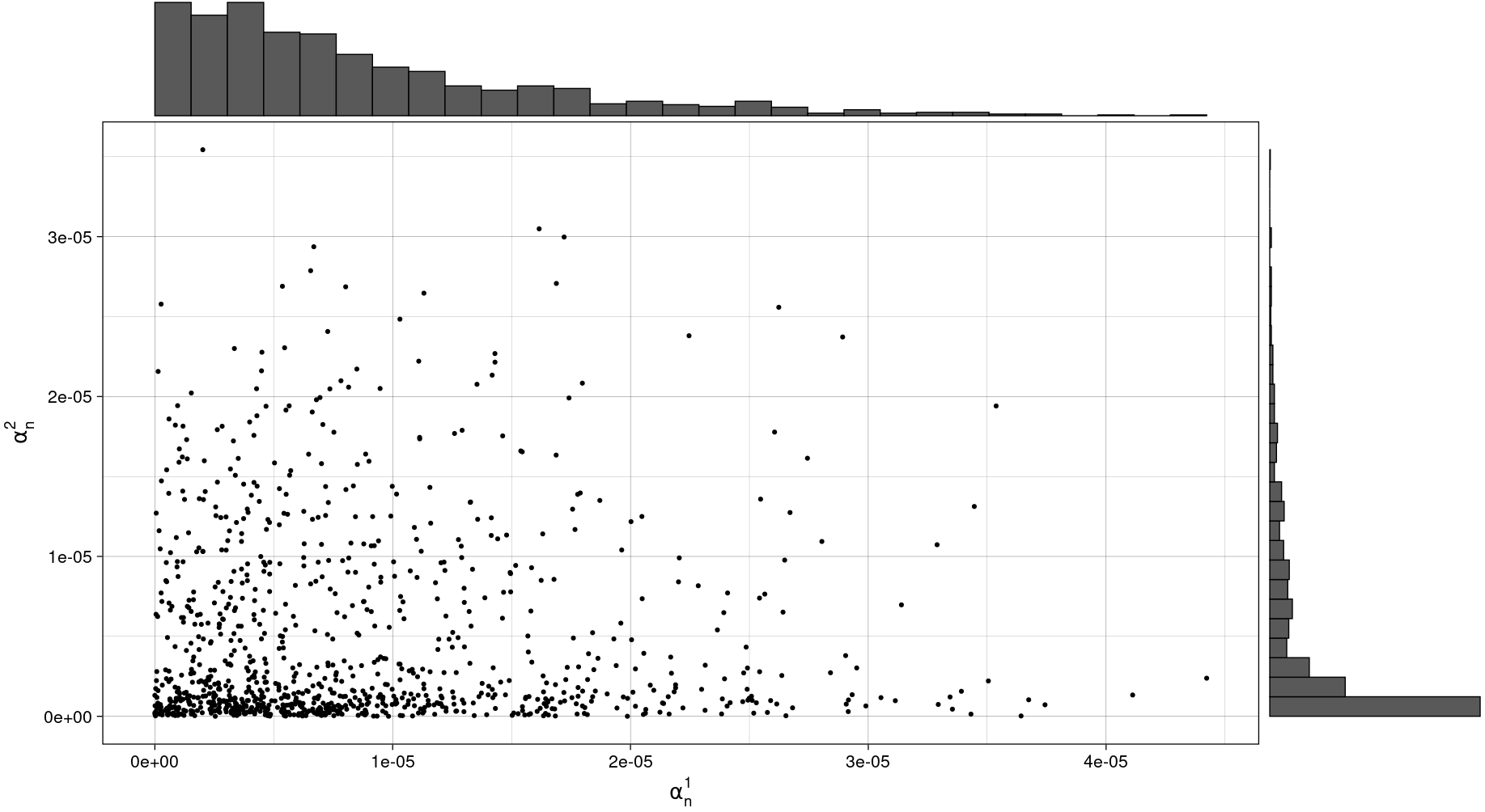
. The histogram of the marginal probability distribution for and are shown on the top and the right.
6 Conclusion
In this paper, we quantify how robust MPE are to model approximations given the degree of approximation in the approximate game. We provide bounds on the degree of approximation based on the approximation error in the reward and transition functions and properties of the value function of the MPE. We also present coarser, instance independent upper bounds, which do not depend of the value function but only depend on the properties of the reward and transition function of the approximate game. Using these approximation bounds, we provide sample complexity bounds for computing an approximate MPE using a generative model.
An interesting feature of the results is that the approximation bounds depend on the choice of the metric on probability spaces. We work with a class of metrics known as IPMs and specialize our results for two specific choices of IPMs: total variation distance and Wasserstein distance. However, the results are applicable to any IPM. For games with high-dimensional state spaces, metrics such as maximum mean discrepancy (Sriperumbudur et al. 2008) might be more appropriate.
The generative model setting considered in this paper circumvents the exploration problem of learning. Therefore, the sample complexity results presented in this paper should be viewed as a lower bound on the number of samples required by an algorithm to learn an -MPE. The proposed algorithm is not practical as it requires storing the transition matrix, which has a size of , which is exponential in the number of agents. The algorithm also assumes that there is a system planner which computes the approximate MPE. Developing a scalable and distributing algorithm for learning MPE remains a challenging open problem.
We conclude by noting that the results presented in this paper were restricted to Markov games with perfect information. An interesting future direction is to develop similar approximation bounds for Markov games with imperfect information as well as specific classes of dynamic games such as mean-field games and their variants.
Compliance with Ethical Standards: Conflict of Interest Statement
The authors declare that they have no conflict of interest.
Data Availability Statement
Data sharing not applicable to this article as no datasets were generated or analysed during the current study.
Appendix A Proof of Theorem 3.1
Let denote the optimal value function for MDP and denote the value function for policy in MDP . Let be the optimal policy for and be an -optimal policy for . From triangle inequality, we have
| (42) |
Now we bound the three terms separately. For the first term, we have
where relies on the fact that , follows from triangle inequality, and follows from the definition of and . Therefore,
| (43) |
For the second term of (42), we have
| (44) |
since is an -optimal policy of .
Appendix B Proof of Theorem 3.2
We follow the same notation as in Appendix A. In addition, let and denote the Bellman operators for the true model and let and denote the Bellman operators for the approximate model. As in Appendix A, the approximation error can be bounded as
| (46) |
Recall that and . Moreover, . Therefore, from triangle inequality, we have
| (47) |
where from the contraction property of the Bellman operators. Rearranging terms and using (44), we get that
| (48) |
Now the first term in (48) can be simplified similar to (43), where in step of (43), we need to add and subtract . Using this, we would obtain
| (49) |
The last term in (48) can be simplified as follows:
| (50) |
The result of Theorem 3.2 follows by substituting (49) and (50) in (48). ∎
References
- Acemoglu and Robinson (2001) D. Acemoglu and J. A. Robinson. A theory of political transitions. American Economic Review, 91(4):938–963, 2001.
- Agarwal et al. (2020) A. Agarwal, S. Kakade, and L. F. Yang. Model-based reinforcement learning with a generative model is minimax optimal. In Conference on Learning Theory, pages 67–83. PMLR, 2020.
- Aguirregabiria and Mira (2007) V. Aguirregabiria and P. Mira. Sequential estimation of dynamic discrete games. Econometrica, 75(1):1–53, 2007.
- Akchurina (2010) N. Akchurina. Multi-agent reinforcement learning algorithms. PhD thesis, University of Paderborn, 2010.
- Albright and Winston (1979) S. C. Albright and W. Winston. A birth–death model of advertising and pricing. Advances in Applied Probability, 11(1):134–152, 1979.
- Altman (1999) E. Altman. Constrained Markov decision processes: stochastic modeling. CRC Press, 1999.
- Azar et al. (2013) M. G. Azar, R. Munos, and H. J. Kappen. Minimax PAC bounds on the sample complexity of reinforcement learning with a generative model. Machine learning, 91(3):325–349, 2013.
- Bajari et al. (2007) P. Bajari, C. L. Benkard, and J. Levin. Estimating dynamic models of imperfect competition. Econometrica, 75(5):1331–1370, 2007.
- Başar and Bernhard (2008) T. Başar and P. Bernhard. H-infinity optimal control and related minimax design problems: a dynamic game approach. Springer Science & Business Media, 2008.
- Başar and Zaccour (2018) T. Başar and G. Zaccour, editors. Handbook of Dynamic Game Theory. Springer International Publishing, 2018.
- Bertsekas (2017) D. P. Bertsekas. Dynamic programming and optimal control. Belmont, MA: Athena Scientific, 2017.
- Breton (1991) M. Breton. Algorithms for Stochastic Games, pages 45–57. Springer, 1991.
- Busoniu et al. (2008) L. Busoniu, R. Babuska, and B. De Schutter. A comprehensive survey of multiagent reinforcement learning. IEEE Transactions on Systems, Man, and Cybernetics, Part C (Applications and Reviews), 38(2):156–172, 2008.
- Cesa-Bianchi and Lugosi (2006) N. Cesa-Bianchi and G. Lugosi. Prediction, learning, and games. Cambridge university press, 2006.
- Deng et al. (2021) X. Deng, Y. Li, D. H. Mguni, J. Wang, and Y. Yang. On the complexity of computing markov perfect equilibrium in general-sum stochastic games. arXiv preprint arXiv:2109.01795, 2021.
- Doraszelski and Escobar (2010) U. Doraszelski and J. F. Escobar. A theory of regular Markov perfect equilibria in dynamic stochastic games: Genericity, stability, and purification. Theoretical Economics, 5(3):369–402, 2010. ISSN 1555-7561.
- Ericson and Pakes (1995) R. Ericson and A. Pakes. Markov-perfect industry dynamics: A framework for empirical work. The Review of economic studies, 62(1):53–82, 1995.
- Fershtiman and Pakes (2000) C. Fershtiman and A. Pakes. A dynamic oligopoly with collusion and price wars. The RAND Journal of Economics, 31(2):207–236, 2000.
- Filar and Vrieze (1996) J. Filar and K. Vrieze. Competitive Markov Decision Processes. Springer, New York, NY, 1996. ISBN 978-1-4612-8481-9 978-1-4612-4054-9.
- Filar et al. (1991) J. A. Filar, T. A. Schultz, F. Thuijsman, and O. Vrieze. Nonlinear programming and stationary equilibria in stochastic games. Mathematical Programming, 50(1):227–237, 1991.
- Fink (1964) A. M. Fink. Equilibrium in a stochastic $n$-person game. Hiroshima Mathematical Journal, 28(1), 1964.
- Herings and Peeters (2010) P. J.-J. Herings and R. Peeters. Homotopy methods to compute equilibria in game theory. Economic Theory, 42(1):119–156, 2010.
- Herings et al. (2004) P. J.-J. Herings, R. J. Peeters, et al. Stationary equilibria in stochastic games: Structure, selection, and computation. Journal of Economic Theory, 118(1):32–60, 2004.
- Hinderer (2005) K. Hinderer. Lipschitz continuity of value functions in Markovian decision processes. Mathematical Methods of Operations Research, 62(1):3–22, Sep 2005. ISSN 1432-5217.
- Hoffman and Karp (1966) A. J. Hoffman and R. M. Karp. On nonterminating stochastic games. Management Science, 12(5):359–370, 1966.
- Jaśkiewicz and Nowak (2014) A. Jaśkiewicz and A. S. Nowak. Robust Markov perfect equilibria. Journal of Mathematical Analysis and Applications, 419(2):1322–1332, 2014.
- Kakade (2003) S. M. Kakade. On the sample complexity of reinforcement learning. PhD thesis, University College, London, 2003.
- Kearns and Singh (1999) M. Kearns and S. Singh. Finite-sample convergence rates for q-learning and indirect algorithms. In Advances in neural information processing systems, pages 996–1002, 1999.
- Krupnik et al. (2019) O. Krupnik, I. Mordatch, and A. Tamar. Multi-agent reinforcement learning with multi-step generative models. arXiv preprint arXiv:1901.10251, Nov. 2019.
- Leonardos et al. (2021) S. Leonardos, W. Overman, I. Panageas, and G. Piliouras. Global convergence of multi-agent policy gradient in markov potential games. arXiv preprint arXiv:2106.01969, 2021.
- Li et al. (2020) G. Li, Y. Wei, Y. Chi, Y. Gu, and Y. Chen. Breaking the sample size barrier in model-based reinforcement learning with a generative model. Advances in neural information processing systems, 33, 2020.
- Littman (1994) M. L. Littman. Markov games as a framework for multi-agent reinforcement learning. In International Conference on Machine Learning, pages 157–163. Elsevier, 1994.
- Littman (2001) M. L. Littman. Value-function reinforcement learning in Markov games. Cognitive systems research, 2(1):55–66, 2001.
- Mailath and Samuelson (2006) G. J. Mailath and L. Samuelson. Repeated Games and Reputations: Long-Run Relationships. Oxford University Press, 2006.
- Maskin and Tirole (1988a) E. Maskin and J. Tirole. A theory of dynamic oligopoly, I: Overview and quantity competition with large fixed costs. Econometrica: Journal of the Econometric Society, pages 549–569, 1988a.
- Maskin and Tirole (1988b) E. Maskin and J. Tirole. A theory of dynamic oligopoly, II: Price competition, kinked demand curves, and edgeworth cycles. Econometrica: Journal of the Econometric Society, pages 571–599, 1988b.
- Maskin and Tirole (2001) E. Maskin and J. Tirole. Markov perfect equilibrium: I. observable actions. Journal of Economic Theory, 100(2):191–219, 2001.
- Müller (1997) A. Müller. How does the value function of a Markov decision process depend on the transition probabilities? Mathematics of Operations Research, 22(4):872–885, 1997.
- Müller (1997) A. Müller. Integral probability metrics and their generating classes of functions. Advances in Applied Probability, 29(2):429–443, 1997.
- Pakes et al. (2007) A. Pakes, M. Ostrovsky, and S. Berry. Simple estimators for the parameters of discrete dynamic games (with entry/exit examples). the RAND Journal of Economics, 38(2):373–399, 2007.
- Pérolat et al. (2017) J. Pérolat, F. Strub, B. Piot, and O. Pietquin. Learning Nash equilibrium for general-sum Markov games from batch data. In Artificial Intelligence and Statistics, pages 232–241. PMLR, 2017.
- Pesendorfer and Schmidt-Dengler (2008) M. Pesendorfer and P. Schmidt-Dengler. Asymptotic least squares estimators for dynamic games. The Review of Economic Studies, 75(3):901–928, 2008.
- Prasad et al. (2015) H. Prasad, P. LA, and S. Bhatnagar. Two-timescale algorithms for learning Nash equilibria in general-sum stochastic games. In Proceedings of the 2015 International Conference on Autonomous Agents and Multiagent Systems, pages 1371–1379, 2015.
- Rogers (1969) P. D. Rogers. Nonzero-sum stochastic games. PhD thesis, University of California, Berkeley, 1969.
- Sengupta et al. (2019) S. Sengupta, A. Chowdhary, D. Huang, and S. Kambhampati. General sum markov games for strategic detection of advanced persistent threats using moving target defense in cloud networks. In International Conference on Decision and Game Theory for Security, pages 492–512. Springer, 2019.
- Shapley (1953) L. S. Shapley. Stochastic games. Proceedings of the National Academy of Sciences, 39(10):1095–1100, 1953.
- Shoham et al. (2003) Y. Shoham, R. Powers, and T. Grenager. Multi-agent reinforcement learning: a critical survey. Technical report, Stanford University, 2003.
- Sidford et al. (2018) A. Sidford, M. Wang, X. Wu, L. F. Yang, and Y. Ye. Near-optimal time and sample complexities for solving markov decision processes with a generative model. In Proceedings of the 32nd International Conference on Neural Information Processing Systems, pages 5192–5202, 2018.
- Sidford et al. (2020) A. Sidford, M. Wang, L. Yang, and Y. Ye. Solving discounted stochastic two-player games with near-optimal time and sample complexity. In International Conference on Artificial Intelligence and Statistics, pages 2992–3002. PMLR, 2020.
- Solan (2021) E. Solan. A Course in Stochastic Game Theory. Cambridge University Press, 2021.
- Song et al. (2021) Z. Song, S. Mei, and Y. Bai. When can we learn general-sum markov games with a large number of players sample-efficiently? arXiv preprint arXiv:2110.04184, 2021.
- Sriperumbudur et al. (2008) B. K. Sriperumbudur, A. Gretton, K. Fukumizu, G. R. G. Lanckriet, and B. Schölkopf. Injective Hilbert space embeddings of probability measures. In Conference on Learning Theory, 2008.
- Subramanian et al. (2022) J. Subramanian, A. Sinha, R. Seraj, and A. Mahajan. Approximate information state for approximate planning and reinforcement learning in partially observed systems. J. Mach. Learn. Res., 23:12–1, 2022.
- Sutton (1990) R. S. Sutton. Integrated architectures for learning, planning, and reacting based on approximating dynamic programming. In International Conference on Machine Learning, pages 216–224. San Francisco (CA), 1990.
- Takahashi (1964) M. Takahashi. Equilibrium points of stochastic non-cooperative -person games. Hiroshima Mathematical Journal, 28(1), Jan. 1964.
- Tidball and Altman (1996) M. M. Tidball and E. Altman. Approximations in dynamic zero-sum games I. SIAM Journal on Control and Optimization, 34(1):311–328, Jan. 1996.
- Tidball et al. (1997) M. M. Tidball, O. Pourtallier, and E. Altman. Approximations in dynamic zero-sum games II. SIAM Journal on Control and Optimization, 35(6):2101–2117, Nov. 1997.
- Vrieze (1987) O. J. Vrieze. Stochastic games with finite state and action spaces. CWI, Jan. 1987. ISBN 978-90-6196-313-4.
- Wang et al. (2019) T. Wang, X. Bao, I. Clavera, J. Hoang, Y. Wen, E. Langlois, S. Zhang, G. Zhang, P. Abbeel, and J. Ba. Benchmarking Model-Based Reinforcement Learning. arXiv preprint arXiv:1907.02057, July 2019.
- Whitt (1980) W. Whitt. Representation and approximation of noncooperative sequential games. SIAM Journal on Control and Optimization, 18(1):33–48, 1980.
- Zhang et al. (2020) K. Zhang, S. Kakade, T. Basar, and L. Yang. Model-based multi-agent rl in zero-sum Markov games with near-optimal sample complexity. Advances in Neural Information Processing Systems, 33, 2020.
- Zhang et al. (2021a) K. Zhang, Z. Yang, and T. Başar. Multi-agent reinforcement learning: A selective overview of theories and algorithms. Handbook of Reinforcement Learning and Control, pages 321–384, 2021a.
- Zhang et al. (2021b) R. Zhang, Z. Ren, and N. Li. Gradient play in multi-agent markov stochastic games: Stationary points and convergence. arXiv e-prints, pages arXiv–2106, 2021b.
- Zhang et al. (2021c) W. Zhang, X. Wang, J. Shen, and M. Zhou. Model-based Multi-agent Policy Optimization with Adaptive Opponent-wise Rollouts. In International Joint Conference on Artificial Intelligence. Montreal, Canada, 2021c.
- Zinkevich et al. (2006) M. Zinkevich, A. Greenwald, and M. Littman. Cyclic equilibria in Markov games. In Neural Information Processing Systems, pages 1641–1648, 2006.