An Analytic Treatment of Underdamped Axionic Blue Isocurvature Perturbations
Abstract
Previous computations of strongly blue tilted axionic isocurvature spectra were computed in the parametric region in which the lightest time-dependent mass is smaller than the Hubble expansion rate during inflation, leading to an overdamped time evolution. Here we present the strongly blue tilted axionic isocurvature spectrum in an underdamped time evolution parametric regime. Somewhat surprisingly, there exist parametric regions with a strong resonant spectral behavior that leads to a rich isocurvature spectral shape. We focus on computing this resonant spectrum analytically in a large parametric region amenable to such computations. Because the spectrum is sensitive to nonperturbative classical field dynamics, a wide variety of analytic techniques are used including a time-space effective potential obtained by integrating out high frequency fluctuations.
I Introduction
Axions are well motivated from the perspective as being a solution to the strong CP problem (Kim:2008hd; DiLuzio:2020wdo; Peccei:2010ed; Peccei:2006as) where the experimental bounds (see e.g. (Agrawal:2017cmd)) have pushed the Peccei-Quinn (PQ) symmetry breaking scale to large values such that the axions are extremely weakly interacting with the Standard Model (SM). The largeness of at the same time presents an opportunity for axions to be the dominant component of the cosmological dark matter both from the perspective of its interaction strengths and the cosmological energy density (Kawasaki:2013ae; Kolb:1990vq; Marsh:2015xka; Sikivie:2006ni; Preskill:1982cy; Abbott:1982af; Dine:1982ah; Berezhiani:1992rk; Sakharov:1994id; Khlopov:1999tm). Since axions are important from both particle physics as well as cosmological perspectives, several experiments have been devoted to its search (B_hre_2013; 2017; Ouellet_2019; Braine_2020; Gramolin_2020; Kwon_2021; Brubaker_2017; mcallister2017organ; alesini2017klash; Alesini_2021; geraci2017progress; Budker_2014; Brun_2019; Armengaud_2014; Armengaud2019). A few reviews on direct detection can be found here (ringwald2012exploring; Redondo_2011; Ringwald_2014; Stadnik_2017; carosi2013probing; Graham_2013) and one can also refer to recent reports (agrawal2021feeblyinteracting; Irastorza_2018) for a list of various experimental searches and methods.
In most popular axion scenarios where a SM singlet field obtains a large vacuum expectation value (VEV) to fix , the potential for the singlet has a quartic term, which makes the fast roll to its minimum during inflation if where is the expansion rate during inflation. In such cases, inflation driven by a different field than completes well after settles to the minimum of the potential. In these situations where the axions are spectator fields during inflation, the isocurvature spectrum associated with the axion field is nearly scale invariant. The weakness of the axion interactions with the SM fields allow the axion isocurvature perturbations to survive thermalization to be observable through cosmological observables such as the CMB and galaxy surveys. Production of spectator axion isocurvature perturbations, its model dependences and associated observational constraints have been widely studied (Kasuya2009; Kasuya1997; Kawasaki1995; Nakayama2015; Harigaya2015; Kadota2014; Kitajima2014; Kawasaki2014; Higaki2014; Jeong2013; Kobayashi2013; Kasuya2009a; Hamann2009; Hertzberg2008; Beltran2006; Fox2004; Estevez2016; Kearney2016; Nomura2015; Kadota2015; Hikage2012; Langlois2003; Mollerach1990; Axenides1983; Jo2020; Iso2021; Bae2018; Visinelli2017; Takeuchi2014; Bucher:2000hy).
The work of (Kasuya:2009up) has pointed out that if the PQ charged SM singlet moves along a flat direction lifted only by masses of that is typical in supersymmetric embeddings of the SM, then because the amplitude of the isocurvature perturbations are proportional to the isocurvature fluctuations of the spectator axion fields can have a strongly blue tilt. Such situations allow the isocurvature to be negligible on large scales probed by the cosmic microwave background (CMB) yet become large on short length scales. Unlike the compensated isocurvature perturbations (Grin_2011; Mu_oz_2016; Gordon_2009; He_2015) which hide the total matter gravitational effects at linear order, the strongly blue isocurvature perturbations can give large gravitational effects at linear order on short length scales. Also, unlike the phenomena explored in works such as (Dimastrogiovanni_2016) where the mass field mixing effects with the curvature perturbations lead to observables, here we are exploring situations where the mass field is stable similar to the ideas of (Linde_1997) and can be observed gravitationally in standard probes such as CMB and large scale structure. Besides being important for the completion of QCD axion phenomenology, a discovery of a strongly blue tilted isocurvature spectra will generically indicate the existence of a dynamical degree of freedom during inflation which has a time dependent mass, quite model-independently (Chung:2015tha). The transition region from the strongly blue tilted region to the flat region of the isocurvature spectra within the supersymmetric axion model of (Kasuya:2009up) was investigated by (Chung:2016wvv). All of the previous computations of the spectrum focused on the overdamped scenarios in which the mass of flat direction is smaller than . Even in the fits to data that were done in (Planck:2018jri; Chung:2017uzc), the parameters were restricted to overdamped scenarios because the spectrum was naively expected to be negligible in the underdamped scenarios.
In this paper, we compute the strongly blue axionic isocurvature spectrum in the underdamped case where the mass of flat direction is larger than , focusing on a parametric region where both the spectral shape is interesting and analytic computation is possible. Somewhat surprisingly, the isocurvature spectrum can exhibit a set of rich spectral resonant shapes with a large enhancement in the amplitude that crucially depends on the underdamped nature of the dynamics. Because the spectrum in this resonant parametric region depends on non-perturbative classical dynamics of , a set of nonperturbative mathematical methods is employed to obtain the analytic spectrum. These include piecewise polynomial solutions to differential equations in a couple of time regions and piecewise effective time-space potential (ETSP) modeling after integrating out fast oscillations. This allowed us to compute a transfer matrix solution to the isocurvature mode equations. Because of this lack of perturbativity, the derivation of analytic expressions as well as the results are quite lengthy.11 1 A Mathematica package to evaluate the spectrum using the analytic methods is given in “https://pages.physics.wisc.edu/~stadepalli/Blue-Axion-IsoCurvSpec-Underdamped.nb”. The readers interested in just the main results can refer to Eq. (242) where the quantity that is most cumbersome to evaluate is as explained there.
Intuitively, the isocurvature spectral range that we can give our analytic results is for the wave vector range where the heavy modes can be decoupled in the axionic model of our interest with multiple degrees of freedom. For the interesting oscillatory part of the spectrum arising from a resonance of background field dynamics, we focus on the parametric region where the velocity of the flat direction field is below a particular critical amount to avoid heavy mode mixing and the background field dynamics becoming chaotic. Due to the already extreme length of the present paper, we defer the discussion of chaotic dynamics and numerical fitting functions that may be useful for data applications to a separate paper. The intuition behind why there is an interesting resonance in the underdamped scenarios while such resonances do not occur in overdamped scenarios is because the overdamped scenarios have field dynamics characterized by exponentials of the form (where is a time parameter and is a mass squared parameter for the flat direction during the initial period) which turns into resonant oscillation producing for the underdamped case. This factor which has a zero will allow the field to reach a dynamically interesting small field region while the kinetic energy is enhanced by an expansion parameter , which translates to a factor of at least an large enhancement in the spectral amplitude over a range of values when compared to the overdamped scenario. Additionally, the resonance condition has the initial condition dependent coincidence requirement of interaction induced mixing between two dynamical degrees of freedom being efficient as will be explained.
Although several of our plots are given with reference to a parameter related to the QCD axion, it is written to divide out the effects of the QCD phase transition. Hence, all of our results can easily be used with the axion field interpreted as a general axion-like-particle.
The order of presentation will be as follows. After a brief review of the underlying axion model in Sec. II, we explain in Sec. III the decoupling of the heavy modes that can be viewed as the main characterization of the analytic formula presented in this work. Sec. IV explains one of the technically difficult part of this work: analytically computing the time when the resonant transition occurs. Sec. V presents the parameterization of the ETSP that results from integrating out the fast oscillations of the classical background fields (which still exists after decoupling heavy quantum modes). Sec. VI maps the parameters of the previous section to the underlying axion model parameter space spanned by { and explains the derivation of the isocurvature spectrum without making assumptions about how many large dips there are in the ETSP. Sec. VII presents a closed form analytic expressions for the isocurvature power spectrum in a certain restricted region of the underlying model space supporting a single large dip in the ETSP. Sec. VIII explains how the isocurvature spectrum changes as the axion model parameters are varied. Sec. IX summarizes this work. An extensive set of appendix sections contain some of the details omitted in the main text.
Appendix A contains an alternative method of computing a critical time required for the isocurvature computations. It serves as an independent check of the computation of presented in Sec. IV. Appendix B describes how the less striking non-resonant situations can be computed within this paper’s framework. Appendix C describes a method from (UVoscillations) of integrating out the fast oscillations to obtain an effective differential equation containing smaller frequencies. Appendix D discusses the dynamics of a composite field object that will be useful in integrating out fast oscillations in the axion model of interest in this paper. Appendix E applies the results of Appendix C and D to integrate out the fast oscillations in the axion model. Appendix F describes the crucial dynamics associated with the lightest eigenvector rotation that will be helpful in constructing the ETSP of Sec. V as well as the maps to the space in Sec. VI. Appendix G describes the time dependence of the lightest mass eigenvalue which will be useful in constructing the ETSP as well as the parametric map in Sec. VI. Appendix H describes the form of the ETSP parameterization used in Sec. V. Appendix I discusses the slowly varying part of the lightest mass squared eigenvalue function that governs the physics of one of the parameters of Sec. V. Appendix J explains the details of the effects coming from the heavy modes considered in Sec. III.
II A brief review of blue axionic isocurvature perturbations
In (Kasuya:2009up), a supersymmetric axion model is studied with the following well known renormalizable superpotential
| (1) |
where the subscripts on indicate global Peccei-Quinn (PQ) charges. Note that this is also the most general renormalizable superpotential transforming under a as
| (2) |
| (3) |
| (4) |
The F-term potential is
| (5) |
A special property of this class of potentials is the existence of flat directions: i.e. in this particular model, it is
| (6) |
The existence of this flat direction is important because this is the reason why the effective PQ parameters will be rolling with a mass of order during inflation (instead of being much heavier and having already settled down), taking advantage of the inflationary -problem: i.e. the Kaehler potential induced scalar potential is
| (7) |
where are positive constants. The parameter dominantly controls the blue spectral index. This setup implicitly assumes that the inflaton sector can be arranged to have such that the flat directions are only lifted by the quadratic terms at the renormalizable level.
Looking along the flat direction of Eq. (6), we set . The resulting relevant effective potential during inflation is
| (8) |
During inflation, the minimum of lies at
| (9) | ||||
| (10) |
The key initial condition is that starts out away from the minimum with a magnitude much larger than and rolls towards the minimum during inflation. This implies the symmetry is broken during inflation. Hence, there will be a linear combination of the phases of which will be the Nambu-Goldstone boson associated with the broken . In particular, with the parameterization
| (11) |
where and are real, the axion is
| (12) |
while the heavier combination
| (13) |
is governed by the potential
| (14) |
Since the field is heavy (i.e. ), it is not dynamically important. Hence, one can gain some intuition for how the axion composition time evolves by setting . When is large, the axion is dominantly and later when becomes comparable to , the axion is a mixture of and .
According to model (Kasuya:2009up), the background equations are as follows.
| (15) | ||||
| (16) |
where has been phase rotated to be real (which is referred to as in (Chung:2016wvv)).
The background system can be rescaled as follows
| (17) | ||||
| (18) |
where
| (19) |
| (20) |
| (21) |
and
| (22) |
The mode equations can be written in these coordinates as (Chung:2016wvv)
| (23) |
where
| (24) |
| (25) |
where and the mass matrix can be rewritten as
| (26) |
Note that we are neglecting the slow roll effects since the in models where this scenario is of greatest interest is negligibly small during most of inflation. Note also that as explained in (Chung:2015pga), Eq. (23) represents the non-sourced part of the isocurvature modes: i.e. the isocurvature modes. The full field contains gravitational infall inhomogeneities sourced by the adiabatic inflaton inhomogeneities.
The expression for the isocurvature can be written as
| (27) |
| (28) |
| (29) | |||||
| (30) |
where and and is the time just before QCD phase transition22 2 The fields have settled down long before this..
The background field equations Eq. (18) control the behavior of isocurvature modes of Eq. (23). Hence, to understand the isocurvature modes, we need to understand the solution space of Eq. (18) in addition to solving Eq. (23). In the parametric region of , the background solutions only have a single bump deviation from the time behavior of the lightest mass squared eigenvalue rising with a constant log slope connecting to a plateau region in space.
starts from a near Planckian value (but restricted to sub-Planckian to have a good chance of the EFT being valid) and moves towards in the approximate solution
| (31) |
where we have labeled the initial time as and
| (32) |
| (33) |
while stays near which is the approximate minimum of the potential. Hence, during the initial time period, the background fields (whose nonzero VEV breaks PQ symmetry) reduce to a single radial degree of freedom. The potentially interesting and nontrivial aspect of this background system’s time evolution occurs in two cases: a) when reaches during the time when ; b) when the energy transfer from to becomes significant (this will be quantified in Sec. IV.3). Both of these time periods are dynamically potentially interesting because the mass matrix undergoes transitions such that the mass eigenvalues and the eigenvectors have time variations that are nonadiabatic (change fast compared to time scale of ). As we will explain, in most cases, only event b) leaves significant imprints on the isocurvature spectrum .
III Decoupling
The dimensionality of the mass matrix indicates that there are two different mass modes. The key dS physics is that at late times, the massive eigenmodes decay away while the lighter mode is important. This means that we do not care about the full equations but only the projected equation onto the lightest eigenvector. Let
| (34) |
where are real normalized eigenvectors of with the the modes being the lighter eigenvalue mode.33 3 For example, when have reached the values corresponding to Eq. (9), the lightest eigenvector is (35) We will call this the instantaneous normalized eigenvector basis. The mode Eq. (23) becomes
| (36) |
| (37) |
| (38) |
| (39) |
where are the time dependent eigenvalues of . One can solve Eq. (37) formally using the Green’s function satisfying
| (40) |
This gives
| (41) |
where is the solution to . Putting this into Eq. (36) gives
| (42) |
This is the integro-differential equation that needs to be solved with Bunch-Davies (BD) boundary conditions to compute the isocurvature perturbations.
There are two independent solutions to Eq (42), both of which are excited to some extent by the quantization with BD boundary conditions. However, the heavy mode is not excited appreciably for the BD boundary conditions as has been checked explicitly. Hence, we focus on the mode with the boundary condition with an initial magnitude of which means
| (43) |
In this case, we see that the right hand side (RHS) of Eq (42) can be neglected for the evolution of as long as
| (44) |
Before the two fields transition at when the mass eigenvalues change as a function of time nonadiabatically 44 4 The transition is defined in Sec. IV.2., we can estimate and
| (45) |
which means that Eq. (44) is satisfied and can be neglected. On the other hand, at , the RHS of Eq (42) may be important since at that time there is only one scale of in the system. During this transition time, the time width of the transition is fixed by
| (46) |
The heavy mixing effect is then quantified in the vicinity of in terms of a new parameter defined in Sec. J as
| (47) |
where and HM stands for Heavy-Mixing.
One can then show that as long as (Refer to Sec. (J))
| (48) |
the effect of heavy mode mixing and the associated RHS of Eq. (42) can be neglected. Close to transition, as tends to , becomes negative due to nonperturbative effects of while the heavier mass eigenvalue . The details of the physics and the derivation are discussed in Appendix J. Therefore, we shall work with only those cases that satisfy the condition in Eq. (48). Later we will express these cases more explicitly in terms of the Lagrangian parameters.
IV Behavior of near the first crossing of
For analytically solvable cases, the details of near the time when
| (49) |
for the first time will be important. Hence, in this section, we provide an analytic approximation of this time behavior.
IV.1 Perturbative solution
For the system can be solved by making the following expansion:
| (50) |
| (51) |
where the near Planck scale initial conditions for gives rise to the prominence of justifying , the near flat direction solution that we seek fixes the power for , and the rest of the powers are simply increasing powers where we omit some of them (such as in expansion) because they will not contribute (as one can check by introducing them). In other words, one can consider the expansion in defined here to be that of smallness of
| (52) |
which is valid over a finite time interval before .
Putting Eqs. (50) and (51) into Eqs. (17) and (18) and collecting powers of , we find the following:
| (53) |
| (54) |
| (55) | ||||
| (56) |
The order has a simple solution identical to Eq. (31) which can also be rewritten as
| (57) |
where
| (58) |
The matching order solution is
| (59) |
Note that when initially does not have much kinetic energy (i.e. ), takes on values that monotonically decrease from to order unity as increases from to . The order also has a simple, local solution:
| (60) |
The order has a nonlocal solution:
| (61) |
| (62) |
| (63) |
Nonetheless, this perturbative expansion by design breaks down near since the hierarchy represented by is lost.
Interestingly enough, the correction to
| (64) |
is which means that the ratio of the next to leading order to the leading order is . In contrast, the next to leading order to leading order ratio for is . To understand this, note that unlike in the equation of motion for is the exact solution to Eq. (17) if . In contrast, is not the exact solution to Eq. (18) with . This means that even though the perturbative expansion of Eqs. (50) and (51) for both break down at , the approximation for breaks down faster in the region
| (65) |
corresponding to an error of the leading order approximation in this region being
| (66) |

IV.2 Beyond perturbation theory
Because the background solutions are sensitive to the details of and the perturbation theory breaks down when (see Eq. (52)), we need a method to solve for the background fields more accurately at . As we will justify later, because most interesting isocurvature spectral behavior comes from the models in which is near a zero crossing (i.e. ), this section will mainly focus on such cases. We will mainly use the method of interpolation using a cubic order polynomial between the time when the perturbation in starts to break down and . We will also check this method in Appendix A using a Taylor expansion approach.
The interpolation polynomial is parameterized as
| (67) | ||||
| (68) |
where we choose to be the time when begins to deviate significantly (to be defined) from . We will then choose the interpolation point taken to be the midpoint between and based on the idea that such a choice approximately minimizes set of competing errors.55 5 Since this midpoint choice is an ansatz, we will actually choose the midpoint between and where defined below is close to . The coefficients will be constrained at through the original differential equations.
In choosing the time to be where the perturbative solution starts to break down, we expect the deviation to come from the neglect of the in the zeroth order perturbative solution. Hence, we set to be the time when
| (69) |
where parameterizes the accuracy we want to achieve in the approximation. For concreteness, we will take in the analysis below. To solve this equation analytically in a closed form, it is useful to obtain a polynomial form. Hence we expand about where
| (70) |
or equivalently
| (71) |
where is defined by Eq. (58) and assume that near is well described by a quadratic expansion of about . We will justify this through self-consistency after the analysis.
To simplify the parametric dependence, define a new dimensionless parameter describing the slope of the zero crossing:
| (72) | ||||
| (73) |
In terms of initial conditions and , the parameter can be expressed as
| (74) |
Putting Eqs. (57) and (59) into Eq. (69), we obtain
| (75) |
where the above expansion is valid for . We now choose the interpolation point to be the midpoint
| (76) |
which in most cases will be a point that lies in the interval .66 6 In situations where coincides with , one can increase the value of to achieve the desired interpolation.
We then obtain 8 equations to solve for the 8 coefficients of Eqs. (67) and (68) using the background differential Eqs. (17), (18), and the values and the derivatives of the perturbative solutions Eqs.(57) and (59). Solving for these coefficients, we obtain
| (77) | ||||
| (78) | ||||
| (79) | ||||
| (80) | ||||
| (81) | ||||
| (82) |
| (83) | ||||
| (84) |
| (85) |
where
| (86) | ||||
| (87) |
| (88) |
and are defined by Eqs. (67) and (68) with the cubic terms dropped: e.g. . Note that since we are using the perturbative solutions (i.e. Eqs. (57) and (59)) for Eqs. (77) through (80), we cannot make too small (otherwise, the perturbative solutions will be unjustified). To address this and as a general check, we also solve the background system using a Taylor expansion method in Appendix A. We find reasonable agreement with the current method if we take .

Now that the background solution is approximately fixed, we can use Eqs. (67) and (68) to solve for the crossing time and the field value there: i.e. solve for . A plot of is given in Fig. 2, showing that for , the crossing occurs when . In terms of and , we obtain the following equations for and by fitting to examples obtained from the analytic expressions:
| (89) | ||||
| (90) |
By the self-consistency of the solution and the method of construction involving Eq. (75), the time itself is away from . Note that as becomes small, increases such that the cubic polynomial expansion of the background fields in Eqs. (67) and (68) is insufficient and higher order terms become significant. Hence the cubic expansion nonperturbative method utilized here is valid when
| (91) |
where . Expanding around yields:
| (92) |
which gives us the following lower bound on
| (93) |
For and we obtain serving as a reasonable cutoff for a 20% accurate computation.
In Sec. III, we remarked that as long as , the decoupling of the lighter and heavier modes is justified. Fig. 25 in Appendix J suggests that this is true when is less than an upper bound given as . Using we infer that the decoupling is satisfied at the first crossing of the background fields for
| (94) |
Later in Appendix E, we will show that this upper bound is consistent with another analytic procedure where we integrate out the high frequency UV modes. Thus, the nonperturbative methods and the analytic techniques utilized in this paper are applicable within a specific parameteric region defined by the parameter . Henceforth in this paper, we will limit ourselves to the study of underdamped axionic isocurvature power spectrum applicable to those cases where
| (95) |
Interestingly, both the lower and upper bounds are nearly -independent for , implying that the parameter is a suitable parameterization for studying resonant underdamped isocurvature modes. Because we will be interested in resonant cases (to be defined below), will never be very small in the cases of our main interest. For completeness, the small cases () are discussed in Appendix B.
Additionally, using the Eqs. (67) and (68) we note that the flat-deviation at the crossing . This is a unique feature of the underdamped scenario where the flat-deviation can tend to if the background fields cross close to the zero-crossing (). Post , the flat-deviation oscillates rapidly with a frequency of and an ) amplitude that decays in time with the Hubble friction. These rapid oscillations are identified as resonance. Accordingly, the axion mode function is now characterized by the scale dynamics till the flat-deviation decays or becomes insignificant. This is unlike the overdamped or non-resonant scenarios where the flat-deviation is negligible and the mode amplitude dynamics is defined primarily by the scale throughout.
IV.3 Resonant scenarios
In this work, we focus on initial conditions where the and initially follow the flat direction of the potential. This corresponds to the initial trajectories approximated by of Eq. (57) for which the flat deviation . For certain parametric cases, there is a significant force on by through when the two fields meet. Such forces cause displacements of towards the “steep” direction in the potential where is significant. This in turn causes strong oscillatory behavior of both and the order unity coupled .77 7 The term “strong oscillatory” here refers to the frequency being much larger than that of . We now present a quantitative condition for this class of scenarios which we call resonant scenarios.
During each when , the effective coupling force on can be expressed as
| (96) |
whose magnitude measures deviation of from the flat direction trajectory. This deviation is a sufficient condition for the force in the “steep” direction to be significant. Hence, we define resonant scenarios to be the cases in which
- 1.
- 2.
where is the first that satisfies these conditions. The first of the conditions ensures sufficient coupling force so that deviates significantly from the perturbed solution while the second condition here is required for to oscillate with an amplitude whose significance is determined by the choice of . For specificity, we will choose .
In summary, we can define to be the time at which
| (97) |
for which has a large kinetic energy and a large deviation from the flat direction. In this paper, we restrict ourselves to only those cases where the fields transition at the first crossing. Therefore and hence forth we drop the notation for crossing/transition. While this choice may seem very restrictive, in principle the model presented in this paper is still applicable to other cases where does not correspond to (under certain conditions). Such cases will be studied in a separate paper (futurepaper).
V Numerically Motivated model
After the transition time defined in Eq. (97), the field takes a large dip towards the negative direction. During a time period surrounding , the effective mass squared eigenvalues in the instantaneously diagonal mass matrix basis has a large dip of . We can capture this behavior in terms of an approximate step function when solving the mode equation in the background of this system.
| (98) |
To model this, define the effective mass squared in instantaneous normalized eigenvector basis shown in Eq. (98) as
| (99) |
where is the lightest eigenvalue of Eq. (26)
| (100) |
where are the elements of . Because we will be only interested in the long time behavior of the zero mode here, we do not need to solve the mode equation with high time resolution. Hence, we use a double perturbative expansion in amplitude and frequency as explained in Appendix C to separate out the low resolution behavior we are interested in. After integrating out the UV modes, we find an effective IR mode mass squared that has only a small number of features. This is illustrated schematically in Fig. 3. In the context of Eq. (100), combined with being , we see that integrating out the UV modes has generated an effective jump in . As one can see in the figure, the effective is significantly simpler than the original .
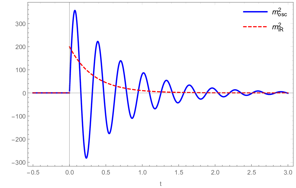
In the step function approximation this can be modeled as
| (101) |
where
| (102) |
and
| (103) |
are the model parameters for this steplike approximation. In particular, is defined as the time when IR averaged makes a negative jump, and is defined as the time after when IR averaged makes a positive jump. Later on, we will see that here represents the step approximation of a smooth decaying nonoscillatory nonequilibrium time-dependent axion mass function whose extinction point corresponds to the PQ symmetry breaking vacuum, where the Goldstone theorem condition is satisfied. The rest of the square well bumps are supposed to be approximations to oscillatory nonequilibrium time-dependent axion mass function. This in turn means that
in this parameterization. Fig. 4 shows a schematic depiction of the mass-model highlighting its key features for a single dip case.
Although this model can in principle be parameterized with an arbitrary number of steplike features controlled by , we will in practice consider at most two such features (i.e. will have at most in this paper where the two dips occur in the intervals and with ). The second dip occurs when where is defined in Eq. (150). It corresponds to the situation where the background fields cross each other again after . Since we choose throughout this paper, there will always be an even number of crossings between the two background fields after . Every such crossing corresponds to a dip in the ETSP within the framework of our mass-model. By limiting the current analysis to two dips, we consider only those cases where a third dip is less than in magnitude. This correponds to all cases where with defined by Eq. (436). Other cases can be treated by including additional steplike features as elucidated previously. With an underlying theory such as Eq. (8), the parameters can be computed in terms of . However, here we will first solve this system analytically, then later express the parameters in terms of }.
V.1 Piecewise solution (scattering matrix approach)
In this subsection, we would like to derive an expression for at some final time given its value at some initial time , assuming that we know the approximate forms of the solution in discrete time regions.
Consider a time region with boundaries . As per this convention, the first region lying between and is termed . The -mode function within any region can be expressed through superposition of linearly independent basis functions :
| (104) |
with the Wronskian . We will take different approximate forms of in each of the regions and match the value and its derivatives at the boundaries to construct in the entire domain as will be described below.
Let us define , , and matrices by rewriting
as
| (105) |
where
| (106) |
and . The coefficients within the region are given by the expression
| (107) |
Here indicates the incoming mode function from the left-hand side. The solution at as the mode exits region is . The mode function at can be constructed as,
where the matrix acts as a scattering-propagator for the mode function from time to through the time slice . The mode function at time after passing through piecewise continuous regions is given as:
| (108) |
V.2 Independent analytic functions in each piecewise-region
We shall now give the general linearly independent basis functions for the form of functions that appear with in our model. Let us consider the following second order ODE as a generic case for mode equation,
| (109) |
In each piecewise region ( in Eq. (101)) of our model, its behavior is either a constant or an exponentially decaying function. Let’s consider these two situations case by case.
- 1.
where can either be positive or negative. For this case, the above ODE has following linearly independent solutions
(110) (111) - 2.
for some arbitrary . The effective frequency squared
(112) now has two different order of decaying exponentials.
A fundamental intuition for these mode function time evolution is that whenever , has a tendency to decay while for the opposite sign, has a tendency to increase. This can be viewed as the result of the equation with having a constant solution (similar to the usual inflationary adiabatic mode) which makes a “point” of criticality in a family of differential equations represented by Eq. (109). This means that the sign of is fundamental to understanding the mode amplitude evolution as a function of time. Moreover, this behavior of mode functions is a fundamental element of quantum fields in curved spacetime.
To solve Eq. (109) analytically, we define an approximate frequency squared as explained below and further divide the region of interest into sub-regions such that the ODE can be approximated as
| (113) |
The idea for the approximation is that competing terms of the form
| (114) |
have only one term dominating except for at most a brief period when the two terms become comparable. During this “comparable” time period, the Taylor expansion of the time dependence is
| (115) | ||||
| (116) |
where we have linearly expanded about the equality time when the and terms are equal. Note that the first of Eq. (114) will dominate over the second term in a time period of . During this time period about , the fractional error between Eq. (116) and the exact Eq. (114) is
| (117) |
which is about 0.2 for the maximum value of that we take below. This lack of sensitivity is an accidental property of the which has a flat region at .
Now, let’s discuss in detail how this approximation is implemented in the model of Eq. (101). At time , there is a jump in the of Eq. (101) due to the term . We will denote the jump amplitude in the effective frequency squared as in this generically parameterized analysis here. Because the term decays faster than the term, will need to take into account the term. We define as the time when term is equal to the full that includes the term. Subsequently, decays according to the approximate expression of Eq. (116). Eventually, the term in will be negligible, and only the term will need to be kept. Since the term decays slower than the approximate in Eq. (116), the expression for will need to be changed to keeping just the term when term equals the term at .
The previous paragraph can be explicitly expressed in terms of the effective frequency equation as
| (118) |
Thus, the time interval is sub-divided into three piecewise regions where each region is characterized by a distinct exponential decay rate such that the system of differential equation in Eq. (109) is now analytically solvable in each sub-region. We define as when are equal
| (119) |
while and are defined as the time boundaries that connect the piecewise regions continuously:
| (120) |
| (121) |
To further improve the accuracy of the above piecewise technique, the amplitude of the exponentials in each sub-region is evaluated as an integrated average of as follows:
| (122) |
where in each sub-region. Using the definition of and the amplitude defined above, the expression for in Eq. (118) simplifies to
| (123) |
In each sub-region now the ODE has a Bessel solution of order for an ETSP of the form :
| (124) | ||||
| (125) |
such that the general solution is a superposition of .
VI Isocurvature spectrum relation to model parameters
In this section, we give analytic expressions for the numerically motivated model parameters and provide isocurvature power spectrum results in certain regions of the underlying model space {. The parameter region is most efficiently divided by introduced in Eq. (72). Small resonance corresponds to the dynamics of the background field with a ) (where defined in Sec. IV.3) that is neither too small (in which case the dynamics is not resonant) or large (in which case, the dynamics becomes difficult to predict due to the large series of nonlinear interactions involved). More precisely, we define this set of resonant cases by Eq. (95):
| (126) |
We present below the analytic formula for the isocurvature spectrum in this corner of the parameter space.
VI.1 General map of analytic model parameters to
As defined previously, the mass-model has following set of parameters:
| (127) |
The final mode amplitude is evaluated in terms of these model parameters. Below we will give a map of these model parameters in terms of and then provide analytic expressions for their evaluations. We limit ourselves to that cover up to double-dip cases in Eq. (101). With the general map is
| (128) | ||||
| (129) | ||||
| (130) | ||||
| (131) | ||||
| (132) | ||||
| (133) |
with the additional second dip for given by the following expressions
| (134) | ||||
| (135) | ||||
| (136) |
Further, the background mass parameter for single and double dip cases is defined as follows
| (137) | ||||
| (138) |
| (139) |
where
| (140) | ||||
| (141) | ||||
| (142) |
| (143) | ||||
| (144) |
| (145) | ||||
| (146) | ||||
| (147) | ||||
| (148) | ||||
| (149) | ||||
| (150) |
where is given in Eq. (415), and and are given in Eq. (419) while . Quite noticeably, the analysis turns very arduous by the addition of a second dip. Precisely for this reason, in Sec. VII we will give closed form analytic expressions for the axion isocurvature spectrum corresponding to single dip cases only. Although we will sketch the motivation and the details of the derivation in the Appendices F, G, H, and I, here we describe the intuition behind this map of the approximation parameters to the underlying model.
The parameter represents the effective axion mass before . During this time the mass is nearly constant because the background fields are following a flat direction such that the potential does not change as the fields change. The dip at is a type of frame dependent eigenvalue rotation mass effect as seen in Eq. (129). It is characterized by the superposition of the and dips close to with a phase separation between the lighter eigenvalue and the corresponding eigenvector rotation gradient effects. The phase separation is dependent. Fields with small tend to have an almost coincident superpositioning of the dips and thus correspond to a small . This -dependence can be understood by referring to the location of the two dips and their subsequent superposition. From Eq. (157) and Appendix F, we infer that the location of the first dip corresponds to the time when the field tends to . Meanwhile Fig. 2 suggests that fields with small transition close to and the dip reaches a minimum soon after transition. Therefore, as increases, the background fields transition farther from such that the separation between the two dips widens resulting in an increased phase separation . For smaller , the two dips are almost coincident resulting in a smaller phase separation.
After the dip, at time , there is a jump in the effective mass squared due to the strong nonlinear interactions through Eq. (21). The jump amplitude is approximately , and after the jump, there is an exponential decay (see Fig. 3) which captures the results of the UV modes that have been integrated out. This UV mode averaging has the effect of multiplying the ETSP by the amplitude of the UV mode divided by the propagator resulting in
| (151) |
represents the next dip whose physics is similar to the first dip modified by the Hubble friction. Meanwhile, the parameter for is a constant of that represents the average mass squared function over the time interval from as detailed in Appendix I. The dynamics of the function is controlled by the slow-varying IR components of the background fields. For it is effectively positive and leads to the decay of the mode amplitude whereas for it is negative and results in mode amplification.
The width of each dip can be evaluated analytically by taking the ratio of the net area under the peak to its maximum amplitude. In principle, the width of a dip increases for larger as the amplitude of each dip decreases. This can be qualitatively understood by the fact that the velocity of the fields governing the dip widths are proportional to the amplitude of the fields which is proportional to the square-root of
| (152) |
Hence, as shown in Appendix F, the dip width can be parameterized as
| (153) |
The fact that the appears in the above expression approximately independently of other parameters is due to the fact that we are focusing on the parametric region where the maximum field excursion parametric dependences are canceled (See Appendix F). Using the analytically obtained polynomial fit for from Appendix F, the width of the first dip can be expressed in terms of as
| (154) |
which highlights that the dip width reduces with an increasing or with the incoming velocity of the field.
A similar expression for the width of the dip is given below:
| (155) |
By rewriting the width in terms of , we obtain the following relation
| (156) |
As expected the width of the dip is broader than the width of the first dip. For small scenarios, the width of the dip is nearly equivalent to that of the . This situation corresponds to a small phase separation such that the and dips almost coincide.
Next within our model, the logarithmic functional dependence of comes from the exponentially decaying frequency of oscillations as explained in Appendix F.
From above parameter assignments, we shall now give expressions for and . These are defined as follows:
| (157) |
| (158) |
| (159) |
| (160) |
| (161) |
where the fields are as defined in Eqs. (67) and (68). By , we are denoting functions such as are to be evaluated at the specific time when .
Next we estimate the amplitude of the flat-deviation . As shown in Appendix D, can be approximately represented via sinusoidal oscillations that drive the resonant exchange of energy between the and fields. For , we can express as
| (162) |
where and is an approximate frequency of oscillations. In order to determine , we solve for the fields post-transition using another set of cubic polynomials with primed coefficients
| (163) |
where the primed coefficients are used to distinguish between non-primed ones in Eqs. (). The 8 coefficients are evaluated using similar expressions as in Sec. IV.2 where the initial conditions must now be evaluated at the resonant transition time (instead of ) and choose instead the interpolation point (where is defined in Eq. (88)). Finally we evaluate as
| (164) | ||||
| (165) |
For cases where the minima of roughly corresponds to the first minima of , we can estimate by evaluating the location where .
| (166) | ||||
| (167) |
which gives us,
| (168) | ||||
| (169) |
The coefficients turn out to be
| (170) |
| (171) |
| (172) |
and the actual parametric dependence of and with is extremely complicated as can be seen in Sec. IV.2. We show comparison with the numerical results for in Figs. 5 and 6.


Remarkably, despite the complicated parametric dependence of Eq. (172) in terms of , the parametric dependence of in terms of is very simple as can be seen in Fig. 6. For , we can give a third order polynomial fit for the amplitude
| (173) |
where all the dependence is contained in through Eq. (74). In this expression, is not bounded from above by because the determination of or is independent of mode decoupling or ETSP evaluation. Instead the above evaluation is valid as long as the fields can be successfully expressed via a cubic expansion. As gets close to 2, the field becomes much larger than after crossing zero. Correspondingly the field undergoes rapid oscillations due to the heavy mass coming from . These rapid oscillations cannot be captured by the cubic polynomial in and the analytic method described above breaks down. Consequently, the analytic estimation of the minima of soon after is lower than the one obtained numerically as shown in Fig. (6).
Note that depends only on in Eq. (74) because by definition we are neglecting the back reaction from in considering the initial velocity condition of . This type of parameterization is natural since is very large ( in the resonant scenario where we are giving our analytic results. Nonetheless, given that the analytic results are formulaically (as opposed to numerically) fitting the actual background field solutions to polynomials before and after that contain , our analytic results fully capture the dependence in the resonant cases considered here.
We remark that the presence of the dip is implicitly dependent upon the strength of the flat-deviation amplitude . The dip is associated with a second dip which occurs when the two background fields cross each other again after transition at . This second crossing after is controlled by the condition given in Eq. (434) that is dependent upon and . Including the expression for the amplitude from above, we find that the second dip occurs for .
Although the interpolation method used in this analytic result seems somewhat ad hoc, the results are consistent with a more systematic expansion around as described in Appendix A.
VI.2 The isocurvature spectrum
The axion isocurvature spectrum is given in Eq. 27. We note that
| (174) |
where we define and simplify Eq. 27 further in terms of mode function,
| (175) |
The is solved using the model of Eq. (101), the approximations of Sec. V.2, and its associated model parameters of Sec. VI.1. Let’s now sketch the steps involved in a bit more detail.
First, we set up the approximate BD equivalent leading adiabatic order boundary condition for the mode equation at time for modes that satisfy :
| (176) |
where
| (177) |
is the conformal time with the scale factor and evaluate the first scattering matrix of Eq. (108) using the solutions of Sec. V.2 evaluated with Eqs. (110) and (111). Using the solution from for the region we obtain the initial conditions for at , when the nonadiabatic rotation of the mass eigenvector becomes strong. Next until when the mass squared jumps, the solutions used to evaluate are again Eqs. (110) and (111), but with a tachyonic constant mass squared. Afterwards, until time when the rotation of the mass eigenvector becomes strong again, the effective frequency-squared is
| (178) |
(this is what we will call the jump ETSP which is obtained after integrating out the UV modes). The solution in this region to be used in of Eq. (108) is governed by the superposition of Eqs. (124) and (125) via the approximations of the in Eq. (118). The initial conditions at should be modified due to the UV integration (highlighted in Appendix C). This is primarily done by scaling the and its derivative by a matrix as follows:
| (179) |
The region is sub-divided into time intervals whose boundaries are dependent on and the amplitude of the jump ETSP through the Eq. (119). The gentle time dependent changes in exponents are most critical for the intermediate modes that satisfy the condition slightly after the transition time while the jump ETSP is still significant. Starting at time , the cycle repeats with the eigenvector rotation becoming strong, although with a smaller magnitude than at . The final is obtained via Eq. (108) where we select . In our calculations we set and after which the background fields oscillations are negligible.
Next we remark that this model has been constructed using only the lightest mass eigenmodes to keep it analytically tractable. Even then, we see that the analytic results are complicated and borders on “intractable”. Hence, this model is applicable up to a maximum mode before the coupling from the heavier mode becomes significant: i. e.
| (180) |
(where ). However, if becomes sufficiently large far beyond this heavy mode coupling values, the dynamics eventually becomes identical to the usual massless axion dynamics. This usual plateau isocurvature spectrum exists for where
| (181) |
| (182) |
corresponding to the wave vector modes that leave the horizon after the background fields have settled to a fraction of their respective minima. Therefore, the only part of the spectrum that we do not have a prediction for (in this small case) is the range .
In Fig. 7, we give plots of the axion isocurvature spectrum generated by the above mass-model for values , 2.348, and with distinct initial conditions corresponding to increasing values of of , 0.97, and respectively.88 8 The case has a corresponding which is slightly larger than defined in Eq. (94), but since this is only at the cusp of the approximations breaking down, the agreement with the numerical results are reasonable. For comparison, numerically obtained spectrum is also included. From the plots we infer that the mass-model is successful in generating the isocurvature spectrum within the parametric region of applicability. The model generates a blue power spectrum for small modes with an approximate spectral index . The spectrum peaks at the first bump and subsequently undergoes oscillations that quickly die away. As we shall see later the location of the first bump and the frequency of subsequent spectral oscillations (bumps) is related to the transition time . The discrepancies between the numerical and analytic computations are noticeable for modes beyond the first bump because during the time these modes exit the horizon, the axion mass is oscillating with a large amplitude in the resonant scenarios. As an example, consider in Fig. 7 the case of for which the discrepancy is the largest for the -region .
These discrepancies can be explained through the limitations of modeling and the integrating out approximation. More specifically, we noted in Sec. V.2 that the analytic approximation of the ETSP in Eq. (118) to solve the mode function is most critical for these intermediate K-modes as long as the modes leave the horizon while the jump ETSP is still significant. The jump ETSP is obtained after the UV modes have been integrated out as shown previously in Fig. 3 and detailed in Appendix H. In the UV integration procedure, we have made the assumption that the flat-deviation is purely sinusoidal with a constant amplitude and a slow-varying time-dependent frequency . Post UV integration, we averaged out the remaining slow-varying prefactors to obtain a constant amplitude jump ETSP (See Appendix H for details). These assumptions along with a pure harmonic approximation can be insufficient to accurately map the sensitivity of the spectrum to subtle variations of the mass eigenvalue for the intermediate modes that leave the horizon around the same time.
One then concludes that background fields with weaker resonance (since that situation will be less sensitive to the limitations of modeling in general) will show far smaller discrepancy between numerical and analytical spectra for these intermediate modes as observed for . Nonetheless, note that the mass-model successfully generates the distinct feature of a larger second bump and a larger third bump than the first for and , respectively. We will discuss this more in the next section.
VII Explanation of the features of isocurvature spectrum
We will now give analytic expressions for mode functions for a specific class of simplified mass-model. This will allow us to explain the parametric dependence of the isocurvature spectrum at different scales and provide closed form analytic expressions for the isocurvature power spectrum in a certain restricted region of the underlying model space.
For the following discussion, we will restrict ourselves to single dip cases corresponding to . Under this condition, our time-dependent piecewise mass-model in Eq. (101) simplifies to the following form
| (183) |
where the mass-model is now limited to a single dip , an exponentially decaying jump ETSP , and an mass squared term . As explained in Sec. (V.2), the above mass-model is used within the corresponding differential equation of Eq. (109).
Furthermore, as discussed in Sec.(V.2), the above differential equation is analytically intractable for certain modes where the following two terms are of similar order of magnitude at
To solve this system analytically, we sub-divided the time region into regions where either one of the aforementioned two terms is dominant over the other.
Hence, in order to obtain a simplified closed form analytic expression for the isocurvature spectrum for cases, we will utilize the following approach. As a first step, we will evaluate the isocurvature power spectrum with the term neglected. This is clearly applicable to all resonance cases where . This assumption immensely simplifies our model and consequently allows us to obtain tractable analytic expressions. Subsequently, the effect of the jump ETSP is added in the form of a correction factor . Through this two-step procedure, we give an approximate analytic expression for the isocurvature power spectrum which will allow us to discover some important generic features. If one is only interested in the results, we refer the reader to Eqs. (242) and (243). We will now give details regarding the aforementioned approach.
VII.1 Step 1:
When , the mass-model simplifies to
| (184) |
Defining as
| (185) |
Eq. (109) becomes
| (186) |
that has an incoming BD normalized solution
| (187) |
with for .
For the rest of our discussion, we will use the following asymptotic forms of the Hankel function for a real argument :
| (188) |
Next we solve within for a single dip and express the solution at as
| (189) |
with and
| (190) |
Note that Eq. (189) is the simplified result coming from the average value for term within the short interval , while containing the initial kinetic energy information generically satisfies
| (191) |
Next we solve within . To further simplify our evaluations, we consider that for , the effect of the model parameter can be factored in through the exponential decay of the final mode amplitude. Equivalently, consider the differential equation
| (192) |
then the mode function has the following asymptotic solution
| (193) |
where is the solution of Eq. (192) with while is the solution with the term equal to zero. Hence, if we neglect the term and solve for in terms of Bessel functions of order (similar to a massless axion), we obtain the final mode function as follows:
where is the conformal time corresponding to the time (see Eq. (177)) and the factor
| (202) |
accounts for the mode amplitude decay/amplification through a positive/negative parameter as explained previously. Using the simplified expression in Eq. (VII.1), we examine the axion isocurvature spectrum for our model for different ranges.
VII.1.1 Modes that leave the horizon early:
Starting with the above equation, we simplify in terms of ,
| (217) |
Since (see Eq. (191)), the mode amplitude is dominated by rather than its derivative.
| (218) |
where . Observe that the mode amplitude is dependent upon the freezeout Hankel function at such that . At the outset, the isocurvature spectrum appears to have a blue spectral index for these scales. However for , the Hankel function has -dependence as given in Eq. (188). We apply this to the Hankel function in our case where to yield the following -dependence for the power spectrum:
| (219) |
For , the term such that the power spectrum has oscillations in the long wavelength region with a log- dependence. Therefore, one observes deviation of the spectral index from which is sinusoidal in log-. These deviations decay as and become insignificant for large fields or when .
VII.1.2 Scales near the first bump ()
Next we consider modes that approach such that the modes leave the horizon after the axion effective frequency squared undergoes oscillations. We start with the Eq. (VII.1) giving us the mode amplitude :
| (220) |
Since (Eq. (191)), the mode amplitude simplifies as
| (221) |
Putting this into Eq. (175), we find the isocurvature amplitude to be proportional to
| (222) |
The location of the first bump is determined by solving
| (223) |
since one can show that there are no small oscillatory features in the rising part of the spectrum in the region . To solve for the peak , we approximate since to obtain the following transcendental equation for the small limiting case :
| (224) |
| (225) |
where and . Since , the solution to the above expression is nearly independent of or more explicitly the properties such as the amplitude and velocity of the field oscillations after . We obtain the solution of
| (226) |
analytically by expanding in the limit .
Calculations in large limiting case yield similar results by solving an analog of Eq. (224):
| (227) |
leading to
| (228) |
Thus, we have shown that the isocurvature power has the first large bump at approximately
| (229) |
with 25% accuracy. Eq. (229) shows that the location of the first bump is the scale that leaves the horizon at time near the resonant transition time . Since the transition is dependent upon the mass and the initial conditions and (see Eq. (74)), background fields with smaller tend to transition later such that they have a larger . Under these circumstances the corresponding first-bump location will be pushed to even smaller scales and become unobservable due to limitations in the experimental sensitivity of short length scales. This is qualitatively the same as the situation in which , which was the subject of previous works on this topic (Chung:2016wvv).
VII.1.3 Scales that lie within oscillating spectrum:
Next we consider modes satisfying that leave the horizon after the axion effective frequency squared undergoes oscillations. The upper limit for these -modes is set by the heavy mode coupling as elucidated in Eq. (180). Meanwhile, Eq. (VII.1) gives the mode amplitude in the limit to be
| (230) |
Considering that , we can rewrite this expression as
| (231) |
We notice from the above expression that the spectrum oscillates via the term for the intermediate K-modes (scales) about a background with an initial decay envelope proportional to . The amplitude of these oscillations is controlled by the dip amplitude operating for a short time interval (see Eq. (129)), which is largely controlled by the mass squared eigenvalue and eigenvector rotation. Meanwhile, the -spacing of these oscillations is approximately
| (232) | ||||
| (233) |
Therefore, the location of the first bump and the frequency of the first few spectral oscillations are directly related to the transition time of the background fields. This can be understood by the following discussion.
For our simplified model, as the background fields transition, the mass squared dips to a negative ETSP for a time period . For all -modes that are still sub-horizon at transition, the incoming mode amplitude picks up a phase that is dependent upon the momentum of the mode sampled at the transition where . Later when these modes exit the horizon the resulting mode amplitude is oscillatory in -space with a -spacing that is dependent upon the transition time . As a result, the power spectrum for these scales oscillates while the imaginary part of the phase controls the amplitude of these oscillations.
VII.1.4 Scales leave the horizon late:
As remarked near Eq. (181), for the plateau part of the spectrum (), the isocurvature perturbation modes return to the usual massless form. In this case, it is better to work in the final massless axion basis. Because the axion field in Eq. (12) is not normalized canonically, the canonically normalized axion is . This allows us to write the plateau part of the spectrum as
| (234) | ||||
| (235) |
where and we have approximated to be constant (neglecting corrections of slow roll parameters which are typically negligible in the physical scenarios of interest in this scenario). The appearance of in Eq. (235) is merely dividing out the scaling of in Eq. (20) This flat part of the spectrum has also been numerically confirmed.
VII.2 Step 2: Adding correction for the term
Eq. (VII.1) gives the final mode amplitude for axionic isocurvature perturbation for cases consisting of a single dip and a negligible jump ETSP where the effect of the parameter (average of ) is included through the exponential decay factor in Eq. (202). Using the expression for under Eq. (129) and the expression for from Eq. (173), we infer that for scales greater than , the amplitude of the resonant UV oscillations is larger than such that the term cannot be neglected. Below we will briefly discuss the corrections coming from .
Since is positive, its inclusion in Eq. (101) for the mode function leads to a decay of all the modes that are super-horizon at (see the discussion below Eq. (112)). Consequently, a significant leads to a reduction in the isocurvature power spectrum for a range of small modes. On the other hand, for all modes that are sub-horizon at , the effect is significantly diminished since the ETSP decays exponentially with a decay factor of . Another way to understand this correction is to note that a large resonant UV oscillations of the background fields imply a significant interaction energy compared to the mass energy at transition. This increases the effective mass for the perturbation modes thereby reducing their amplitudes.
We now give approximate analytic expressions to include the effect of the jump ETSP to the previously derived isocurvature perturbation mode amplitude. The effect of ETSP is included as
| (236) |
where
| (237) |
with defined as
| (238) | ||||
| (239) | ||||
| (240) |
Note that the expression is primarily derived for all super-horizon modes . Since must tend to for modes that satisfy , we have constructed as a smooth function connecting these two asymptotic values of . Hence, the above correction factor is an interpolated approximation for the intermediate modes lying between the two asymptotic scales. An important consequence of this interpolation is that it does not show a gradual shift in the location of the first bump towards smaller values due to an increasing jump ETSP as can be observed in Fig. 9. To accurately model this gradual shift of the first bump, one needs to evaluate an improved correction factor for the intermediate modes by solving the scattering matrices of Sec. (V.1) with the jump ETSP included explicitly. Furthermore, we remark that is nearly a constant since Eq. (189) and Eq. (190) suggest that
| (241) |
which is independent of for all modes with at .
VII.3 Isocurvature power spectrum
In summary, the isocurvature power spectrum for background fields with (where and are given in Eqs. (93) and (150) respectively) corresponding to a single dip can be expressed (where is defined in Eq. (74)) as follows:
| (242) |
with coefficients given as
| (243) | ||||
| (244) |
where
| (245) |
for , and
| (246) |
which accounts for the mode amplitude decay through the parameter:
for parameters
| (247) |
and given in Eq. (485) which for reduces to
| (248) |
where and its derivative in Eq. (485) for are given in Eq. (419), is given in Eq. (421) and . As noted near Eq. (181), there is a gap in the analytic spectrum in the region . The correction factor is defined in Eq. (236).
The coefficients have been defined such as to be approximately scale-independent. Since , the term in is approximately -independent. Similarly, is independent of for long wavelengths and hence it is absorbed into . Meanwhile gives us the approximate location of the first bump. If is neglected, the term has the following approximate form for ,
| (249) |
where we remark that eventually tends to for extremely small scales that correspond to the massless axion. To evaluate the expressions given in Eqs. (242) and (243) into a numerical amplitude, the parameters can be computed through
| (250) | ||||
| (251) |
| (252) |
| (253) |
obtained from Sec. VI.1. The definition of can be found in Eq. (71), and the variables are the conformal times corresponding to obtained through Eq. (177). In turn, to evaluate in Eq. (250), use Eqs. (73) and (75). To evaluate of Eq. (253), put Eqs. (67) and (68) into Eqs. (448) and (426) and minimize by varying time .
For cases with where a second dip is also significant, the shape of the isocurvature spectrum is modified as the parameter becomes a -dependent function. The modes now carry additional phases that are dependent upon the dynamics of the dip. This situation is similar to the explanation provided in Sec. VI.2. These cases are solved using the scattering matrices of Eq. (108) with the full set of model parameters. Eq. (242) and the more general computational procedure presented in Sec. VI are the main results of this paper.
VII.4 Discussion
By substituting Eqs. (243), and (249) into Eq. (242) we obtain an approximate order of magnitude estimate for the amplitude of the first bump corresponding to for :
| (254) |
where
| (255) |
near and varies slowly (fractional power of ) for . The above expression is an approximation and higher order corrections such as the presence of additional dips (for instance dip due to the second crossing after ) can lead to further increase in the amplitude.
Next, we compare the above expression to a corresponding one for the overdamped scenario. In a previous work (Chung2017), numerical fitting functions were developed to estimate the isocurvature power spectrum for overdamped cases. It was found that the bump amplitude was maximally approximately a factor of 3 compared to the massless axion plateau. However, those fitting functions were evaluated in a corner of parameteric region with such that they were largely independent of up to the required accuracy. In order to include the parametric dependence, we note that within the framework of our mass-model, the overdamped scenario can be studied by considering a single dip followed by the parameter in Eq. (184). Using the cubic-polynomial expressions in Eqs. (67) and (68), it is easy to show that for the overdamped scenario and . Using these estimates, we evaluate the amplitude at first bump as
| (256) |
where it is worth noting that the residual dependence is obtained by fitting the mode amplification due to the slow-varying function. To understand this, note that for the overdamped scenario, the background fields settle to their respective minima along a trajectory where . Hence, the associated function is negative and can lead to amplification of the mode function (see Sec. (I) for further details). Also, note that unlike the underdamped scenario, there is no large kinetic energy at transition and thus the absence of any amplitude enhancing corrections for the overdamped case.
We now compare the isocurvature spectral amplitude between the two cases and obtain
| (257) |
For , the dependence is
| (258) |
which is an approximate numerical value ( accurate) resulting from evaluating as explained below Eq. (253). Thus, the ratio of the isocurvature power spectrum between overdamped ( and underdamped ( scenarios is approximately
| (259) |
At , the above ratio is approximately and hence as and , Eq. (259) tends to unity, giving us a check of the formulas based on the consistency with the results of (Chung2017). Also, Eq. (259) becomes independent for large .
Furthermore, the ratio of the amplitude of first bump to the massless axion plateau is
| (260) |
Note that as , canceling the enhancement factor. Therefore the ratio of the bump amplitudes saturates to a constant for large values. For in the resonant case of our interest, Eq. (253) can be approximated as
| (261) |
which shows how the underdamped scenarios enhance the bump amplitude. This large number ultimately can be traced to the combination of two coincident effects: a) enhancement of the kinetic energy due to a time phase accident in the context of oscillatory background solutions which exists only in the underdamped cases b) -involving interaction energy dominating over the mass energy. For instance, consider the ratio of the kinetic energy to the net potential energy (mass + interaction energy ) at transition for the two cases. Using Eq. (89), we can approximate this ratio for for the resonant underdamped case as follows
| (262) | ||||
| (263) | ||||
| (264) |
where we note that for underdamped resonant cases, the interaction energy is . Remarkably, the parametric dependences have canceled out in Eq. (264).
A similar evaluation for the overdamped situation where the interaction energy is yields
| (265) | ||||
| (266) | ||||
| (267) |
where we note being insignificant in both the numerator and the denominator. Thus, we observe an approximate enhancement in the spectral power for the underdamped cases compared to those of the overdamped. Since, the first bump in overdamped cases is maximally approximately a factor of 3 compared to the massless axion plateau, we obtain an effective enhancement factor of for the underdamped scenario as observed in Eq. (261).
As highlighted previously in Sub-sec. (VII.2), a large jump ETSP leads to an attenuation of spectral power for all modes super-horizon at while having a decreasingly small effect on the sub-horizon modes. An interesting consequence of this is that for large enough , the amplitude of a subsequent bump (second or higher) can appear much greater than the first bump. This can be understood as follows. From Eq. (242), we infer that the amplitude of the spectral bumps (oscillations) in the absence of the jump ETSP can be expressed as
| (268) |
where is the amplitude of the first-bump and is independent of .
With the inclusion of , the spectral power for all super-horizon modes at is attenuated due to a dependent correction factor as shown in Sec. VII.2. For , the corrected spectral amplitude of the first bump can be written as
| (269) |
where the dependence of is approximately a constant for all super-horizon modes. On the other hand, the spectral power in Eq. (242) for the sub-horizon modes have the property :
| (270) |
where and defines mode when the . The smoothly interpolates between and in the spectral region [.
Comparing Eqs. (269) and (270), we conclude that it is possible for certain high modes to have a larger spectral power than the first-bump. Quantitatively, this is true for the following approximate range of modes
| (271) |
This is generically observed as a larger second or third bump than the first (see Fig. 242). The amount of this relative enhancement can be evaluated as:
| (272) |
where the factor of comes from in Eq.(237) for . Hence, the enhancement is approximately proportional to and increases with the scale. Thus, we remark that large ) resonant effects together with any additional dips () corresponding to higher order corrections, can result in spectral power enhancement by a factor greater than the as derived previously for the resonant underdamped cases. Unlike the factor whose origin was discussed in Eq. (264), this high mode enhancement is dependent on the parameter .
VIII Parametric dependences of the isocurvature spectrum
One qualitative predictability difference between the overdamped and underdamped axionic scenarios where the PQ symmetry is broken before the end of inflation stems from the fact that there is an attractor solution for the background fields as well as for the linear perturbations in the overdamped scenarios. This means that given a Lagrangian in overdamped scenarios, the cosmological predictions have less dependence on the initial conditions. As an analogy, in the case of slow roll single field inflation, one only needs to specify the initial field value and not its time derivative to specify a prediction for the observables. For the usual cosmological axion scenarios, the radial field associated with PQ symmetry breaking is considered to be sitting at the minimum of its potential. This means that the only initial condition dependence of the axion isocurvature during inflation is . In the case of the current underdamped scenario of interest, there is an additional phase space dependence of the PQ symmetry breaking radial field directions as well. Because of the non-attractor behavior for the underdamped dynamics along the flat direction, the dominant additional phase space degree of freedom is the initial field value and the kinetic energy of the radial field along the flat direction parameterized by .
In this section we will study the dependence of the axion isocurvature spectrum on the model parameters and the initial conditions . The effect of each parameter variation is discussed keeping all of the others fixed.
VIII.1
The numerical model presented in this paper and the associated axion isocurvature spectrum have been derived for background fields within the parametric region given by . Above the upper bound , the analytic methods utilized in this paper break down due to the significant heavy-mode mixing from Eq. (48) at , and at around the same upper bound, the adiabatic approximation technique also breaks down.99 9 Beyond , the background fields will cross at least twice after transition. For large , these crossings can occur close enough such that effective heavy mixing from the superposition of each crossing becomes significant. Moreover, as , the background field dynamics turns highly chaotic after transition and a closed form prediction of the mode amplitude in terms of is not feasible. Field configurations with large tend to fall under this category. These configurations associated with and the accompanying isocurvature spectrum are a subject of interest and will be explored in a separate companion paper (futurepaper). For less than the lower bound, the cubic polynomial expansion of the background fields is insufficient and higher order terms become significant. The parameter can be computed as a function of underlying Lagrangian model parameters and the initial conditions from Eq. (73).

In Fig. 10 we plot the dependence of within the range of Eq. (95) close to corresponding to the range of values where is close to (but before) the first zero-crossing of the field.1010 10 Recall is approximately equal to before . The monotonic increase in is captured through the following expression:
| (273) |
Next, in Fig. 11, we present isocurvature spectra for three different values. We remark that as is increased, the field rolls down faster owing to the frequency .1111 11 The exact dependence of the velocity on is dependent on whether the system is in the resonant, non-resonant, overdamped, underdamped situations. Here, we will here be focusing only on the resonant cases, which is the main focus of our work. Consequently, the first zero-crossing of the field occurs earlier with an increasing (See Eq. (71)). This in turn increases the factor controlling leading to a larger kinetic energy at . The larger kinetic energy is later converted into the interaction energy at transition whose larger value is responsible for the growth of the isocurvature amplitude through the resonant effects. Hence, increasing 1212 12 See below regarding how much one can increase . results in an amplification of first bump in the isocurvature spectrum. Moreover, an increasing height of the isocurvature spectrum is accompanied by a receding location of the first bump towards lower values. This is again explained by decreasing as is increased because Eq. (229) implies
| (274) |
When one compares the first bump amplitude to the plateau amplitude in the case of Fig. 11, one sees that the ratio can be about 30. This is already explained in Eq. (261) of Sec. VII.4 where we evaluated an enhancement factor of
| (275) |
for modes lying within the range compared to the modes in the massless axion plateau region of the spectrum ().
To understand this qualitatively, one first notes that there is the possibility in the underdamped scenarios of a large kinetic energy in the falling when the interaction with becomes strong. This large kinetic energy leads to nonadiabatic effects post such that the axion mode amplitude obtains an enhancement compared to an overdamped scenario.
Note in Fig. 11 that the frequency of the -space oscillations also increase with . This has already been explained quantitatively in Eq. (233). To understand this another way qualitatively, note that the temporarily negative lightest mass squared eigenvalue and the nonadiabatic rotation of the lightest eigenvector pump the mode amplitude (see Eq. (26)). Therefore, the space oscillation frequency is reflective of the nonadiabaticity producing mode dynamics at time where the modes have the characteristic phase , giving a -space oscillation period of as can be seen explicitly in Eq. (233).
The examples presented in this paper are limited to a range of values where the transition occurs close to the first zero-crossing. One might then worry that the mass model is no longer applicable for higher values because according to Fig. 10, the value naively seems to increase to violate the approximation methods used. However, as we will discuss in a separate paper (futurepaper), is a discontinuous function of . As we will show there, the present mass model is still applicable for a range of larger values (although the regions where the model is applicable are not continuously connected).
VIII.2
The dependence of the isocurvature spectrum is multi-faceted. The term in Eq. (245), which is mostly about the normalization of the axion field, suggests a proportionality of the power spectrum. This is an expected result since the time-dependent massive axion isocurvature spectrum has a dependence within the long wavelength region (as well as in both the plateau regions). Thus, the variation of the power spectrum in the massless plateau region has an proportionality similar to the overdamped scenario.
For scales that lie within the oscillating part of the spectrum, additional dependences arise from the and terms of Eq. (242). As shown in Sec. VII.4, the spectrum in this region has the following proportionality
| (276) |
Using the analytic expressions derived previously, the ratio has the following polynomial form within the parametric region given by Eq. (95),
| (277) |
where and . With all other parameters fixed, we have the relationship . Including the term, the power spectrum has the following effective dependence in the oscillating region
| (278) |
where
| (279) |
As becomes large, the power spectrum tends to the expected proportionality. One can understand this by noting that for all other parameters fixed, an increase in results in a rapid reduction in such that can subsequently become smaller than . This is an interesting behavior which can be explained more clearly by noting that for resonant underdamped fields, occurs close to the zero-crossing:
| (280) |
At , the field is and the strong coupling force and resulting in . Using Eq. (72) and , we deduce that the parameter in Eq. (277) is associated with whereas is related to the integral of the coupling term . Fig. 12 shows plots of power spectra for a fixed value with different scales highlighting a reduction of the power spectrum for .

VIII.3
Next we consider the dependence of the power spectrum. We will consider two situations here. In the first, we discuss fields with such that the fields evolve after the transition without any crossings. This situation gives rise to a slowly-varying . The second case is where the fields have large resonant amplitude such that the fields cross each other at least once after . As explained in the Appendix I, such a crossing results in a situation where the field settles to its minimum from below (). Due to this unique alignment, the function now becomes negative as the fields settle to their minima asymptotically. In both cases we shall see that the spectrum increases for smaller values with the essential dynamics dictated by the settling of during different temporal phases. The discussion is limited to .
Let us now consider the first case. The function results in an approximate exponential decay of the mode amplitude through the
| (281) |
factor where the integral is evaluated through the Eq. (492). The integral can be divided into two temporal phases. During the first phase, the dominant field rolls down from its peak amplitude with a decay constant equal to . Later as the fields get closer to their minima during the second phase, the decay constant increases by nearly a factor of four to . Since starts out close to and eventually settles to zero, the integral is dominated by the first phase. In this first phase, behaves as the flat direction mass which decreases with decreasing, resulting in : i.e. a smaller results in a larger effective mode amplitude.

In the second case, the field approaches its minimum from below. Unlike the previous case, the first temporal phase is insignificant due to the oscillating IR fields and a dominant ETSP. Hence, the effective mode amplification due to the negative is brought about during the second phase through Eq. (281). As decreases, decreases much slower due to the exponential decay rate of . Moreover, a smaller results in a larger value of . As a result of these two effects, we see from Eq. (281) that the mode function undergoes larger amplification. This is shown in Fig. 13.
VIII.4 and

Here we discuss the parameters and that define the initial conditions for the underdamped rolling fields. Varying these initial conditions directly alter and the value of . Hence, the effect of these two parameters is best understood by studying the expression from Eq. (74). We consider the minimal case with and expand to quadratic order in in Eq. (74)
| (282) |
We discover that has a local minimum at evinced by the absence of the linear term in . This is expected since an increase in the initial kinetic energy leads to a larger at the zero-crossing. As seen in Fig. 14, the dependence of on in Eq. (74) is nonlinear beyond the quadratic nonlinearities in Eq. (282). As seen in Eq. (282), the parameter leads to a monotonic increase in the value of within the range of Eq. (95) with the intuition that the initial energy is increased as in the intuition for the increase. A representative set of values as a function of is shown in Fig. 14.
As is continually increased, becomes nearer to the next higher zero-crossing time, thereby reducing the overall spectral power. Similarly, if is continually increased then the transition time moves to the next higher zero-crossing time. The subsequent height of the power spectrum can be analyzed by evaluating the value of at the new transition. Due to the length of this paper and the natural parametric scope of small in this paper, we discuss the isocurvature spectra reflecting higher zero-crossing of in a separate companion paper (futurepaper).
IX Summary
In this paper, we provided an analytic expression for the blue axionic isocurvature spectrum in the underdamped nonequilibrium axion scenarios for a particular parametric region corresponding to a mild amplitude () of resonantly oscillating PQ symmetry-breaking radial fields. The main expression given by Eq. (242) exhibits an amplitude of Eq. (243) and an oscillating spectrum whose -space oscillation period is of the order the value of the first -break location in the spectrum (Eq. (229)). Remarkably, the first bump amplitude of the spectrum is enhanced by a factor of compared to the plateau amplitude of the spectrum associated with the massless axions as explained near Eq. (264). Furthermore, in some cases with large ) resonant effects, the spectral power can receive larger than the enhancement of the first peak as explained near Eq. (272).1313 13 Here we have scaled the PQ symmetry breaking parameter as where is a quartic coupling and is the Hubble expansion rate during inflation. In contrast, for the overdamped nonequilibrium axion scenarios (see (Chung:2016wvv)), the relative amplitude ratio is only a factor of few (maximally approximately a factor of 3). The -oscillation spacing is reflective of the mode amplitude-setting dynamics at time whose phase is , giving a -space oscillation period of .
Technically, the computation was carried out using a combination of a parametric restriction where the heavy modes are decoupled (Sec. J), perturbation theory (Sec. IV.1), analytic fitting to polynomials in the nonperturbative region (Sec. IV.2), piecewise ETSP modeling (Eq. (101)), and the technique of integrating out fast oscillations (Appendix C). This allowed us to compute a transfer matrix solution to the isocurvature mode equations (Eq. (108)). Overall, based on comparing to sample numerical calculations, the accuracy of the computation is about 20%-50% with set to 0.2. Most of the uncertainty is coming from the technique of integrating out the fast oscillations (for example, estimation of ) and the approximations made regarding the IR components of the fields after the transition at . A Mathematica package to evaluate the spectrum using the analytic methods can be accessed from “https://pages.physics.wisc.edu/~stadepalli/Blue-Axion-IsoCurvSpec-Underdamped.nb”. Even though the analytic formula is complicated, compared to the pure numerical solver, the speedup factor is about .
In this paper, we have focused on presenting analytic spectral results in the resonant oscillatory -range for moderate values, where characterizes the velocity of the falling field near the transition time (see Eq. (72)). This would be helpful even if a purely numerical approach to the problem were to be used in data fitting since this will serve as a solvable check on the system. In a companion paper (futurepaper), we will present results for larger situations in the high limit to complete the understanding of the possibly observable blue isocurvature spectra. In such cases, there are no purely analytic results, but there will appear a novel stochastic model that parameterizes the small range amplitude variation with . In that paper, we will also exploit various symmetries to obtain relationships between parameters which is useful more as a transferable technique than quantitative predictions. Finally, we will also defer to that paper a discussion of general fitting functions for this underdamped blue axionic isocurvature class of models that do not refer to underlying Lagrangian parameters .
There are many interesting possible followup topics to be investigated. Recent Planck results (Planck:2018jri) show that axion-like curvaton models with uncorrelated blue-tilted spectrum is the most favored of the isocurvature models. The fits also indicate a possibility of measuring a spectral index of at 95% CL consistently with the recent findings of (Chung:2017uzc). It would be interesting to study whether there are hints of resonant isocurvature spectra presented in this paper in the existing and future data. Another possible usage of this enhanced oscillatory peaks presented in this paper would be to investigate the formation of primordial black holes similar to the investigation of the curvaton models in (Inomata2021; Ando2018; Kawasaki2013; Kawasaki-PBH2013; Bugaev-PBH2013; BUGAEV_2013; Young_2013; Ando:2018nge; Chen_2019; Passaglia:2021jla). Similarly it is equally appealing to study second order gravitational waves and non-gaussianities through either a QCD axion or a curvaton isocurvature mode as in (Kawasaki2021; Kawasaki:2008pa; Ando2018; BUGAEV_2013; Hikage2012; Inomata2021; Inomata2019; Langlois_2011; Beltr_n_2008; Linde_1997).
Acknowledgements.
This work was supported in part by the Ray MacDonald Fund at UW-Madison. We also thank Amol Upadhye for preliminary investigations into this problem.Appendix A Taylor expansion consistency check
In Sec. IV.2, we gave a solution to using an analytic fit to cubic polynomial, utilizing the information from the differential equation and perturbative solution. In this section, as a check, we give an alternate derivation of assuming where satisfies
| (283) |
where
| (284) |
We restrict ourselves to solving the case of the resonant case (see Sec. IV.3) in which
| (285) |
(see Eq. (58) for definition of and Eq. (31) for the initial conditions on ). The reason why we dwell on the accuracy of the value of is because the numerical results in the resonant situations are very sensitive to the value of due to the large and the fact that the complex mode amplitude is sensitive to the time phase of real background field . The solution method presented here involves a combination of perturbation theory, Taylor expansion, and successive linearization approximations. The most difficult aspect of the computation is in estimating the errors associated with the approximation, and it is this feature that the present section’s approach is an advantage from that of Sec. IV.2. However, the formalism here is cumbersome compared to that of Sec. IV.2, and the differential equation solution for used below has limited parametric applicability. The results nonetheless serve as a check on Sec. IV.2 and provides an error estimate.
Since the computation is long, we first give the results:
| (286) |
| (287) |
| (288) |
| (289) |
| (290) |
| (291) |
| (292) |
| (293) |
| (294) |
| (295) |
| (296) |
| (297) |
| (298) |
| (299) |
| (300) |
| (301) |
| (302) |
| (303) |
| (304) |
where is given by Eq. (71) and
| (305) |
This is very insensitive to the parametric details because of the power in
| (306) |
where
| (307) |
and are functions of themselves given in Eqs. (338), (339), and (340). With the fiducial value of without solving for self-consistently, the estimated error on is around 30% for an variation in around . Note that here is the analog of the in Eq. (75), and for is consistent with taking . This is one of the main consistency checks of this appendix on Sec. IV. The parametric dependences of values of this appendix section for near 2.35 agree with the presentation of Sec. IV providing another independent consistency check. If one wants better accuracy, it is straight forward (but tedious) to iterate using Eqs. (287), (363), (361), and (354). One of the most interesting aspects of this is Eq. (382) that shows that 2 and to be a generic prediction in the resonant case. These results can also be viewed as an alternate method of computing that can be combined with Eq. (242) to evaluate the isocurvature spectrum.
The improvement in the solution can be seen by comparing the solid line and long dashed in line in Fig. 16. In the parametric case of
| (308) |
the agreement with numerics is about 6% in (or equivalently about in which illustrates a very high precision in is required to get the to be accurate to 6%). For the more general case, we estimate an error for of less than about 35% assuming that the error in the prediction for dominates. The ratio for this case of Eq. (308) is about 5. The reason why the computation is very sensitive to is because small changes leads to large changes since Eq. (283) implies
| (309) |
where .
In the rest of this section, we derive these results. Readers not interested in the details can skip most of the rest of this section.
A.1 behavior in resonant scenarios
Here, we construct the solution in the region near , where the perturbative expansion Eqs. (50) and (51) break down. The tools we will use to construct this solution are 1) different derivative approximation for different break down at different times ; 2) an expansion of a different differential equation of composite operators that restricts the functional space of about a special point where . Note that the Taylor expansion method of 1) is non-perturbative although very limited in its time-range extension of analytic computation. For sudden transitions that is being studied here, even this limited method yields nearly an order of magnitude improvement in accuracy in the estimate.
A.1.1 Region
As noted when discussing in Eq. (60), the solution becomes a bad solution exponentially fast near . Hence, we will define below a time period just before to match the known Eq. (59) to a finite order polynomial in this time region. The reason why the finite order polynomial will turn out to be a better approximation than the original perturbative solutions will be due to the fact that different Taylor expansion derivative approximation for different break down at different times . We will choose from the condition that the finite order polynomial and be a good approximation at the same time.
Start by a quadratic Taylor expansion of about
| (310) |
We truncate this at the quadratic order and replace the coefficients with leading perturbative solution:
| (311) |
where the error estimate is for the error incurred in matching the Taylor expansion coefficients to derivatives and is the error incurred for the quadratic Taylor expansion truncation to the exact solution. It is important to keep in mind that the left hand side of Eq. (311) is not the approximate but meant to be the exact solution that is valid even at . If one forgets that, then this equation seems like an approximation of as a quadratic function instead of the exact solution in a small neighborhood.
How can a Taylor expansion of do better than keeping the original itself? After all, why stop at just quadratic order in Taylor expansion if one can get higher derivatives using The answer is that each successive derivative Taylor expansion coefficient evaluated at becomes an increasingly poorer approximation of the exact solution’s derivative . We will demonstrate this explicitly.
In matching the exact solution to at , the error incurred for the zeroth order Taylor expansion can be estimated using the perturbative solution Eq. (60) since at , the perturbation of Eq. (60) is still valid
| (312) | ||||
| (313) |
| (314) | ||||
| (315) |
| (316) | ||||
| (317) |
| (318) |
| (319) |
where
| (320) |
| (321) |
| (322) |

In the resonant cases in which is not large enough to destroy the small cosine approximation , we can use the following relationship:
| (323) |
where we have defined
| (324) |
This can be used to rewrite these errors as
| (325) |
where
| (326) |
has been defined to suggest the appropriate scale to understand this expression in the resonant case. Note that although it looks dimensionally wrong, it is actually consistent since we have divided out the scale here. Our final value of computed will determine . Similarly, the error for the higher derivative coefficients are
| (327) |
| (328) |
| (329) |
| (330) |
One can see from Fig. 15 (in which we plot ) how the higher order Taylor expansion coefficients become more uncertain at earlier before reaching . In this numerical example case, we see that to keep the second order Taylor expansion coefficient accurate to about 20%, we need Taylor expand at about . The actual error at can be better than 20% depending on which Taylor expansion term contributes the most.
Hence, we conclude based on coefficient errors alone
| (331) |
| (332) |
| (333) |
| (334) |
| (335) |
| (336) |
In the resonant case, we can expand as before about :
| (337) |
| (338) |
| (339) |
| (340) |
| (341) |
where one should keep in mind that and are of order unity in the resonant scenarios where the expansion involving about the zero crossing of has been made. Since we are evaluating at which is farther away from the zero crossing of this expression is only about 25% accurate. Typically, the term dominates and this large coefficient pushes the error towards larger than unity at . Therefore needs to be made as large as possible to induce the in Eq. (337) to reduce . This is a motivation for having a quadratic Taylor expansion compared to a linear Taylor expansion since generically a Taylor expansion has a larger degree of accuracy for higher order polynomials.1414 14 One might ask, why not then go to even higher orders in Taylor expansion? That is because of Fig. 15 which tells us that the higher order polynomial coefficients are not approximated well for a given expansion point . To rigorously optimize, one would have to minimize the error in the plane where is the degree of polynomial with which one is expanding. However, we will be content with setting and maximizing to approximately minimize the error.
Let’s discuss the competing error incurred from Taylor expanding the exact solution to quadratic order (which is always possible for any analytic solution in a sufficiently small neighborhood):
| (342) |
According to the equation of motion for (Eq. (18)):
| (343) |
Let’s first see why it is a bit delicate to estimate the RHS. We know that the largest contribution to the RHS of Eq. (343) are from the the potential terms near its maximum since :
| (344) |
There is a partial cancellation in this expression since at least at , we have by construction
| (345) |
making
| (346) |
This cancellation fails more and more as becomes smaller and smaller compared to as approaches . This means we expect to be maximized near . On the other hand, since near (since that is where whereas in this region, there is a cancellation which could increase near , making the exact location of the maximum of uncertain. Nonetheless, as long as does not exactly represent the zero of , we expect from these arguments that
| (347) |
which is what we will evaluate now.
Since the RHS of Eq. (344) only involves first derivatives and lower, we can use the assumed solution to evaluate these derivatives:
| (348) |
which when evaluated at is
| (349) |
The derivative can also be evaluated at :
| (350) |
After using Eq. (326), the largest number in is . Hence, we expand in powers of to obtain
| (351) |
where is defined in Eq. (326) and is defined as
| (352) |
where is given by Eq. (71). Note the mass matrix becomes strongly off-diagonal at : i.e.
| (353) |
Because can easily be of order (because of the cubic power) and because can be of order , these two terms can compete. Also, can easily be negative. Hence we arrive at the Taylor expansion error estimate
| (354) |
at . The equivalent fractional error of Taylor expansion is
| (355) |
where
| (356) |
and were defined in Eqs. (284) and (326). This error pushes the choice of towards smaller values (i.e. in the opposite direction of the push by ). To evaluate this error, we need a value of (or equivalently ) which is calculated with fixed. Hence, itself is a function of .
Ideally, we want to compute
| (357) |
to minimize the errors. Because itself depends on , the derivative is tedious to obtain.


The combined error (in absolute values added instead of quadrature) is plotted in Fig. 16.1515 15 Although we could add in quadrature to tighten the error estimates, we here stay conservative both because we do not really know the distribution shape of the errors and we want to keep the algebra simpler. We see that the minimum error occurs when the Taylor expansion point of Eq. (311) is . The expected error for the value of the function is at most around 35%. However, to get the plots (or equivalently, to use Eqs. (337) and (354)), we need to compute for a given model, i.e. using Eqs. (283), (311), and the analogous equation for approximation:
| (358) |
However, in practice this does not need to be done. That is because the minimum error generating is not sensitive to the exact value of . This is illustrated in Fig. 17 where the errors are evaluated with two different estimates of . The Taylor approximation curve is generated by solving for self-consistently by solving
| (359) |
for which is now a function of and evaluating evaluated at . The “naive ” curve is generated by solving
| (360) |
and Eq. (353) is satisfied. Hence, we see gives the minimum error in the parametric case of Fig. 1.


Let’s analyze the sensitivity of to the parameters more generally. Start by rewriting Eq. (337) as
| (361) |
| (362) |
The solution to Eq. (357) is thus
| (363) |
To get an approximation for the solution, we approximate as a smooth polynomial in , note is unimportant, and assume that we are close to the solution of Eq. (357) such that :
| (364) |
Setting this to zero gives
| (365) |
or equivalently
| (366) |
Hence, for we can approximate
| (367) |
Since stays near unity for different and , we see that this varies slowly with different parameters of owing to the power dependence. Hence, we will use the result of Fig. 17 and use
for the resonant cases. This should be a good approximation to about accuracy since power reduces uncertainties to about this level. The variable is the analog of the in Eq. (75), and for is consistent with taking . This appendix has thus provided a consistency check as well as an error estimate of Sec. IV.
A.2 Solving for
Although the value of that minimizes the error is not very sensitive to the value of , we see from the second figure of Fig. 17 that is sensitive to . We defined to be the solution Eq. (283), which is approximately
| (368) | ||||
This equation and Eq. (357) together determine and (where is a parameterization of through Eq. (352)).
Use resonant condition
| (369) |
to turn the trigonometric functions in this expression into polynomials:
| (370) |
Although this equation can be linearized successively to obtain an accurate solution, the algebra becomes significantly simpler with only about loss of precision if we drop the dependence on arising from the exponent
| (371) | ||||
| (372) |
Use successive linearization (effective Newton’s method) to obtain a solution to the simplified nonlinear equation:
| (373) |
| (374) |
| (375) |
where the definition of the rest of the objects are given in Eqs. (289)-(304). These expressions indicate that since for example in the contribution we have contributions such as
| (376) |
in the numerator1616 16 Recall that in the resonant scenarios. with an in the denominator. Also, note that even though looks like it is sensitive to , one can check that there are cancellations when derivative of is computed. This cancellation occurs because if the is chosen in the region where the error of Eq. (311) is minimized, the sensitivity on by construction is minimized.
For example, consider
| (377) |
where is the numerator and is the denominator of Eq. (375). The derivative receives contributions from the numerator and denominator (after combining over a common denominator)
| (378) |
| (379) |
where is a common factor and we have displayed the leading terms1717 17 Leading terms at least for near parametric region. To see the cancellation between these two terms, Eq. (378) can be rewritten using Eq. (352):
| (380) | ||||
| (381) |
Comparing with Eq. (379), we see that the cancellation occurs because
| (382) |
One of the merits of this exercise is to see that this cancellation is independent of in the resonant region considered here. This also allows one to see has to be in the approximate region of the zero of the left hand side of Eq. (382).
In the case of considered in the plots such as 1, dominates over by about a factor of 5. However, since the entire point of this messy exercise was to obtain a good numerical estimate of , we keep . In this parametric point example, we find Eq. (374) to evaluates to
| (383) |
with while the numerical solution for this case is
| (384) |
attesting to a good approximation (about 5% error). Note this also allows us to compute for example
| (385) | ||||
| (386) |
giving
| (387) |
(defined in Eq. (326)) very close to the numerical value of . In evaluating this, we made usage of Eqs. (71) and (32) as well.
The error in the more general case can be estimated as follows. To account for the 35% type of error in the field value, note
| (388) | ||||
| (389) | ||||
| (390) |
which means that the error in shifts by . This is why has to be very accurately determined to obtain .
Appendix B Small
For field configuration where (where is defined in Eq. (93)) at transition, the resonant conditions in Sec. IV.3 are not satisfied. In such cases, the mass eigenvalue and the rotated eigenvector gradient effects are less than post-transition. As a result, the axion mass transitions smoothly from to a massless state. In these cases, the separation between the transition and the zero-crossing is usually . However, by evaluating Eq. (60) at , one finds that the leading order correction . Hence, we see that the perturbative solution is still valid for and the cumbersome nonperturbative computation is no longer necessary for computing the value of the fields at However, to compute the spectrum, still needs to be computed, and this requires an accurate computation of using the nonperturbative computation that we have presented in Sec.IV. Using this and a slowly time-dependent mass squared function , the final mode amplitude can be computed. The absence of resonance and a weak dip less than results in a power spectrum with the long wavelength region plateauing after the first bump without any further noticeable bumps similar to an overdamped scenario.
Appendix C Adiabatic approximation for an oscillating time space potential
Consider the following second order ODE with an oscillating time space potential.
where is a slow-varying envelope function with amplitude while the harmonic oscillations are rapidly varying (large frequency ). The solution of the aforementioned ODE can be approximated by separating into the IR and UV components. As long as this hierarchy can be maintained we can approximate as
| (391) |
whereby represents the slow-varying (IR) adiabatic behavior superimposed with a fast high frequency (UV) noise . Next, we substitute this into our original equation to get,
We now apply the initial conditions. Assuming that the incoming function is at some and has no UV behavior, the slow-varying component will match appropriately with the . The fast-varying will then be matched with or be negligible. Accordingly, over a small time-scale , the UV component will be initially sourced by the incoming IR component
and by assuming a slow-varying envelope function we obtain up to a leading order
Note that and sets the scale of the UV component compared to IR. Next, we substitute the UV solution into our original differential equation and integrate out the UV scale over one time-period
| (392) |
The above differential equation governs the dynamics of the IR component subject to the initial conditions and . By defining , we note that if , then the above UV and IR treatment is also valid up to . Fig. 18 gives plots of and obtained by solving the exact ode and its adiabatically reduced form respectively.
Appendix D Flat-deviation
The quantity defines a deviation from the flat direction. This is a crucial measure as it controls the strongly coupled dynamics of the two fields. To obtain a differential equation for we start with the background field Eq. (18). We multiply the two equations with and respectively and add them together to obtain,
which yields an effective equation for the flat-deviation
| (393) |
where are the elements of the matrix. This is an interesting equation in that apart from the kinetic mixing terms on the RHS, the equation for has been made to “look” linear, although it certainly is not because of . Consider an expansion about a neighborhood of defined to be the zero of :
| (394) |
In that neighborhood, the solution must behave as
| (395) |
Since comes time after while has been increasing beyond while has been decreasing towards , we can approximate that has a Taylor expansion in time:
| (396) |
We then find
| (397) |
| (398) |
yielding
| (399) |
We also know
| (400) | ||||
| (401) |
Keeping to zeroth order in , we put into Eq. (393) the zeroth order terms in Eqs. (399) and (401). The resulting Eq. (393) has a solution in the vicinity of
| (402) |
| (403) |
For the remainder of our discussion, we will consider the following approximate expression for the flat-deviation with a constant amplitude and a slow-varying time-dependent frequency
| (404) |
Flat-deviations of occur close to a zero-crossing of characterized by a strong nonlinear interaction between the two background fields. After transition, when the background fields are settling to their minima, the frequency of flat-deviation is . As the fields initially start out along the flat direction, is negligible since . When the fields reach close to the transition, the term causes the fields to deviate away from flat direction. Later when the fields have settled to their minima, the flat-deviation tends to
| (405) |
The kind of dynamic behavior described above can lead to resonance which is characterized by a significant flat-deviation as shown in Fig. 19.
Appendix E UV and IR decomposition of the background fields
Post transition, the background fields are strongly coupled through the interaction term as shown in the equations
| (406) | ||||
| (407) |
where is an oscillating function given in Eq. (404). The dynamics of the coupled system post-transition can be understood in terms of a UV and IR decomposition detailed in Appendix C. If the frequency of the oscillating function is much larger than the root of its amplitude, the system exhibits a hierarchy between the UV and IR states. We may then integrate out the UV degree of freedom and retain the IR components to describe the adiabatic behavior of the coupled system. In principle we can write
| (408) |
where the subscripts represent the slow (IR) and fast (UV) component of the fields.
From Appendix C and assuming (which we will justify below), we can write down an approximate solution for the UV component of the fields as
| (409) |
where we have used Eq. (404) in place of (with a time-dependent frequency term ) and switched the cosine function in Eq. (404) to a sine for convenience. In terms of the UV and IR components we can write flat-deviation as
| (410) | ||||
| (411) |
Meanwhile from Eq. (409) we infer that
| (412) |
subject to the approximation . Thus, we will approximately take the frequency-squared of the function as the sum of the squares of the IR components of the background fields. Since the UV components are smaller in amplitude compared to IR, we obtain an approximate relationship between the IR components of the background fields,
| (413) |
This is an important result which indicates that if the background fields can be factorized into UV and IR components, then the IR components continue to follow the flat direction.
Post transition, begins to increase due to a positive velocity of and becomes dominant compared to a decreasing . During this time, the UV integrated equation of motion for the IR component of the dominant field is given below
| (414) |
while the smaller field is obtained through the flat direction condition . Note that is a function of the background fields highlighting the non-linearity of the above equation. However, to obtain an analytic solution we will consider an average value for the parameter over a half-oscillation of (since increases up to a maximum and then falls back towards ) such that a general solution to the above damped oscillator equation for a constant average is given as (during the time when the term is not appreciable)
| (415) |
where
| (416) |
| (417) |
for
| (418) | ||||
| (419) |
where properties near can be obtained from Eq. (163). Meanwhile, the field is given by the flat direction
| (420) |
Since is a time-dependent function of the background fields, we apply a semi-numeric approach to estimate an average value of between and the time when for . This choice of allows us to consider both the situations where the two background fields may either cross each other again after or not. The procedure involves matching the analytical solution in Eq. (415) to the numerical results for the fit parameter . Through this procedure we obtain an empirical fit expression for as a function of and :
| (421) |
where
| (422) |
When , the above solution has an oscillating behavior with a maximum frequency
| (423) |
Within our parametric region of interest, the amplitude satisfies from Eq. (173) imposed by . Since the transition occurs close to , the two fields oscillate over the equilibrium scale such that with an average value approximately at . Therefore, we see the self-consistency of the assumption that for . Between and , the system of background fields can be given by the cubic polynomial solution. Also, the IR fields can oscillate momentarily with a frequency while the UV scales oscillate with frequency . Therefore, the hierarchy between the two scales is clearly established.
In summary, prior to transition the fields are best described via primary frequency . After transition, we can separate the fields into UV and IR components as long as . As , the UV component decays away and the IR components settle to the minima. Fig. 20 highlights the above conclusions by showing UV and IR components of the background fields for with all the other parameters set to the set used in Fig. 5.


Appendix F Lightest eigenvector
We will now study the lightest mass eigenvector corresponding to the lightest mass eigenvalue and derive analytical expression for . We begin by defining the lightest mass eigenvector,
| (424) |
where the column matrix elements are
| (425) |
with the definition
We would like to evaluate the derivative squared term . Using the definitions from above, we note that and so that . By defining we expand ,
| (426) |
with
| (427) |
Thus, peak amplitude is related to the relative velocity of the two fields as they cross each other. The peak is maximized if the two fields approach from opposite directions thus maximizing the relative velocity. Upon substituting the analytical form of into Eq. 426 and solving we obtain that the first maxima close to occurs when the field is approximately . The maximum amplitude is given as,
As , we have so that we can expand in terms of which simplifies
| (428) |
which has a limiting case
| (429) |
Using the above analytical expressions, we present a second order polynomial fit in terms of parameter for the Eq. 428 in the range
| (430) |
As the field rapidly rolls down from the Plank scale, the first peak peak occurs slightly before transition and is characterized by the the dominant frequency. After transition, the fields can be divided in to the UV and IR components. When the jump ETSP in Eq. (414) is significant at , it leads to an frequency oscillations of the IR fields (see appendix E) such that the fields cross again after transition (also characterized by the zeros of ). Quantitatively, this is equivalent to since . Thus, we can obtain approximate location of the second crossing of the background fields by solving Eq. (415) for the time when .
Since additional crossings require a significant jump ETSP, we begin with the Eq. (415) for the background field and evaluate an approximate condition for the background fields to cross after transition. As we are interested in cases where the crossings are caused by the jump ETSP, we will neglect the term in Eq. (414). Hence, we consider the following equation
| (431) |
which has the general solution
| (432) |
where the primed coefficients are obtained similar to the below Eq.(415) and is a function of .
As , we look for the minimum value of such that . Hence, we equate
| (433) |
Since , we reduce the above expression to
| (434) |
Eq. (434) gives us an approximate minimum value of such that the two background fields cross each other after . For and , we find that the minimum value of saturates to about
| (435) |
where The term in Eq. (434) can be evaluated using the nonperturbative cubic polynomial expansion for the background fields from Eqs. (67) and (68) around . The minimum value of that satisfies the conditional equality in Eq. (434) is defined as . It corresponds to a parameteric cutoff such that for , the background fields cross each other again after . For (corresponding to the fiducial parameter set ), we obtain . Similarly, for a much larger value of , we obtain highlighting that reduces with . If the resonance amplitude is large enough, the background fields can cross each other more than once after . This corresponds to the situation where
| (436) |
where corresponds to the second zero of . Further, we remind that each crossing of the background fields corresponds to a peak which is modeled as a dip within our numerical mass model in Eq. (101). Since we limit ourselves to just two dips in this paper, we will consider only those cases where .
For cases, the dip within our mass-model can be evaluated using Eq. (426) wherein the peak amplitude of the function around is evaluated by substituting into using solution provided in Eq. (415) and Eq. (420). Meanwhile, the maximum amplitude of these peaks located close to the zeros of requires evaluation of as observed in Eq. (426). In terms of the IR and UV components, we rewrite as
| (437) |
where we identify , , and . Using Eqs. (409), one can show that the mixed terms and cancel out due to an accidental symmetry that exists in the potential governing , while the amplitude of the first derivative of the UV component is given as
| (438) |
Up to a linear order in Taylor expansion, we can approximate in the vicinity of as
| (439) |
Therefore, including the additional contributions from the UV term , we can approximate peak in the vicinity of using
| (440) |
within Eq. (426). Through fitting, we find that up to a error, the above evaluation procedure can be approximated by the following simplified expression:
| (441) |
where refers to the time when the two background field cross each other again after and is evaluated from the cubic polynomial solution for the background fields in Eqs. (67) and (68). These peaks are lower in magnitude due to the Hubble friction as shown in Fig. 21.

Next we note that Eq. 428 can be qualitatively understood by the following factorization
| (442) |
where the coefficients are dimensionless and order . The width of a peak is characterized by
| (443) |
where is the field at the maximum of which gives us
| (444) |
We shall therefore consider the following repatriation for the width
| (445) |
where takes the following form:
| (446) |
Therefore, has parametric dependence on and . As increases, must also increase due to increasing resonance amplitude. On the other hand, the corresponding value of at the location of the peak reduces monotonically with an increasing which results in a smaller . Within the parametric region (), the two competing behaviors are equally important and tend to cancel each other out such that within the region of our interest we can approximate so that the width of the peaks are approximately given as within accuracy. Using Eq. (430) for the into Eq. (445), we obtain the following linear expression in for the width of the first dip
| (447) |
In general, the width of these Gaussian-like peaks can also be evaluated by taking the ratio of the total area under the peak to its maximum amplitude.
Appendix G Lighter mass eigenvalue
In this section, we will study the variation of lightest mass eigenvalue over time. The lightest eigenvalues of the mass matrix is given by the expression
| (448) |
In terms of and we rewrite Eq. (448) as
| (449) |
During the early-phase when and any transient oscillations of are negligible i.e. , reduces to,
As the fields then approach transition, the zero-order approximate perturbative solution is no more valid. The lighter mass eigenvalue transitions from to a negative dip. Post this dip, oscillates due to the resonance before settling down to zero. As explained in Appendix E, the background fields post dip can be factorized in terms of the UV and IR components. Using these components we can write as
| (450) |
such that we can factor out the resonant UV oscillations over the slow-varying background.
Next we substitute the above factorization for into Eq. (449) and expand in powers of ,
Within the parametric region of interest where , we drop all terms of and higher such that
| (451) |
The above expression highlights that the mass eigenvalue thus oscillates in-tandem with the flat-deviation oscillations before settling down to zero. The expansion leading to Eq. (451) is appropriate as long as the term . From Eq. (173) we infer that for , meanwhile and hence the expansion term tends to as . To the contrary, if the two fields tend to momentarily, the above expansion breaks down. However, the lighter mass eigenvalue in those conditions tends to . This situation arises when the trajectory of the two fields tends to be chaotic and unstable which is outside the scope of our parametric region.
Appendix H Building the numerical model
In Appendix G we obtained an approximate expression for the lighter mass eigenvalue in the limit . Next we substitute for the flat-deviation from Eq. 404 into the Eq. 451
| (452) |
where the slow-varying background term of from Eq. (404) has been absorbed within such that
| (453) |
where are the IR components of the fields as given in Appendix E. We identify as a low-frequency axion mass of order that eventually tends to zero when the background fields settle to their respective minima. In this context, the effective axion mass post transition comes from physics at two different frequency/energy scales. In order to obtain an analytically solvable model, it is convenient to integrate out the high frequency terms and obtain an effective low frequency model in terms of the IR components. We begin by redefining after the first dip as follows:
| (454) |
where is the approximate time when the flat-deviation first crosses zero after the initial dip. Thus, up to a quadratic expansion in , in Eq. (452) has the following harmonic expansion
| (455) | ||||
| (456) |
where . Applying the adiabatic approximation method elucidated in Appendix C we integrate out the UV degree of freedom in to yield
| (457) |
where the first term in the above expression comes from the IR reduction of the term linear in in Eq. (452) while the second term is a positive offset due to the term from the quadratic term in Eq. (452). Moreover, while the first term in Eq. (457) results in a modification of the initial conditions at , the second term does not. An important consequence of the IR reduction in Eq. (457) is that the contribution from the linear term cancels out. This cancellation of the first order UV contribution is similar to the one we observed and explained in Appendix F. Thus, the adiabatic reduction approximates the oscillating time space potential in to a nonoscillating exponentially decaying positive time space potential
| (458) |
where the prefactor
| (459) |
Since is a time-varying function, we evaluate an average value for within a half-oscillation of the background fields using as the weighing function.1818 18 Note that this averaging of is different from the procedure we carried out in Appendix E since there we were concerned with a non-linear differential equation of the background fields. Using the analytic solutions for the background fields in Appendix E, we obtain the following approximate empirical fit expression for average :
| (460) |
Note that the above estimation is approximate and hence one of the sources of uncertainty for all modes super-horizon at . With this approximation, the system is now analytically solvable where the reduced low frequency mass-model has a jump ETSP defined as
| (461) |
at . Within the framework of this adiabatic reduction, the axion mode function is expressed in terms of its slow (IR) and fast (UV) components,
| (462) |
where we will neglect the component since (within the scope of the adiabatic reduction). The effective mass squared ( for mode function is now generalized in terms of a low-frequency mass model with a reduced mass eigenvalue in Eq. (458) and the dips (explained in Appendix F) modeled as negative square wells/dips.
The first dip at the transition is obtained through a superposition of the first dip and a corresponding dip due to the evolution of the mass eigenvalue from to an oscillating function (due to a strong resonance between the fields). This explains the first dip of our model given in Eqs. (101) and (129). After this first negative dip of , the effective mass squared is governed by the exponentially decaying positive function of . Once the mass squared function decays away, the parameter of evaluated as an average of the defines the asymptotic behavior of the mode amplitude. The dynamics of function and its effect on the mode amplitude is covered in Appendix I.
Appendix I Effective mass squared function
The effective axion mass after IR averaged makes a positive jump transition at time (see Fig. 4) is derived from physics at two different frequency/energy scales. These are specified by under-damped oscillation of the lightest mass eigenvalue and slowly varying part of the lightest mass squared eigenvalue function given by Eq. (453). In this appendix, we will discuss the function in detail and evaluate its effect on mode amplitude. From Eq. (453) we note that dynamics of is characterized by the motion of IR components of the fields along the flat direction towards the minimum of the potential. Along this direction, the fields can move towards the minimum either from above () or below () as shown in Fig. 23. When the fields have settled to their respective minimum, goes to zero. Interestingly then, if the field settles from above the minimum then the condition is satisfied, while if it moves from below, then subject to a few conditions.
We shall now study this behavior starting from the expression for of Eq. (453) which can be rearranged to get
| (463) |
Next we parameterize
| (464) |
where for moving from above and when moves from below. In terms of the function , Eq. (463) becomes
| (465) |
Hence, we find the following conditional expression for sign for
| (466) |
as mapped in Fig. 22.
Therefore, dependent on the trajectory of a prolonged exponential decay or amplification of the super-horizon axion modes behaves as
| (467) |
where the integral in the exponent is cut off when decays faster than . The lower limit of this integral corresponds to when the exponentially decaying term proportional to in Eq. (101) can be neglected.
In situations where , the magnitude of the gradient of the potential is much smaller when than when . Therefore, the fields evolve slowly ( time scale in -dependent evolution) in the former scenario and fall towards the minimum rapidly in the latter (see Fig. (23)). Accordingly, the axion background mass is significant in the latter case only when the fields are close to the minimum.1919 19 If , then there is no appreciable since the mass squared function time dependence due to the fast rolling fields rapidly diminishes the magnitude of this function.

When the jump ETSP is significant at , it leads to an frequency oscillations of the IR fields (see appendix E). These oscillations cause the fields to cross each other at least twice after the transition. To see this, first note that the resonant conditions force to cross (first crossing) to make . Next, the asymptotic values of these fields are where for , and this fact requires a second crossing. These crossings give rise to a second and third peaks (the first one being at ). Since the crossings occur at approximately (due to the initial conditions making ), we know at the second crossing. For , the interaction energy now decays away due to the Hubble friction while before crosses again. Without the interactions mediated by the flat deviation , the settles towards the minimum from below () and can become significant.
The parametric boundary of when the IR components of the fields cross each other at least once after is set by the following condition provided in Appendix F
The above provides an approximate minimum value of for the background fields to cross again after . Substituting for using Eq. (173) and using Eq. (421), we obtain a cutoff (boundary) in terms of defined to be . Therefore, we will consider and cases separately.
I.1
For the parametric region , the fields will not cross again for . To solve for this system, it is convenient to divide the time regions based on whether or not term is appreciable compared to term in Eq. (414). We will call the region the period when is negligible and the period when is important.
Consider the equation of the field in the region
| (468) |
where we can safely neglect the effect from the asymptotic term . The solution to the above equation is given in Eq. (415) in Appendix E while is given by the flat direction condition in Eq. (420).
Due to a large positive velocity at , the reaches a maximum and then moves slowly towards the minimum with an initial exponential decay rate equal to
| (469) |
During this period when we can expand using Eq. (453):
| (470) | ||||
| (471) |
Note that as , the ratio gradually decreases. As the two fields then approach closer to their respective minima, the interaction term becomes important starting at time , and the decay rate changes. Therefore, the integral corresponding to the exponential decay of the super-horizon mode amplitude during the first temporal phase where the field has an exponential decay factor given by Eq. (469) is
| (472) |
where
| (473) |
and is the time when the -mode becomes super-horizon i.e. . Thus, modes that exit the horizon before transition () have a K-independent decay factor. The time is when the jump ETSP has decayed and becomes negligible compared to .
Next, we consider the time period where the term is non-negligible compared to . By comparing the two terms and using the flat direction , we make an approximate choice of as when
| (474) |
such that
| (475) |
where additionally we note that at
| (476) |
To derive field equations, we consider the field displacements as
| (477) |
that implies
| (478) |
in which case the terms quadratic in can be neglected compared to with the minima of the fields located at
| (479) |
Expand the expressions in equations of motion Eqs. (17) and (18) in terms of to yield
where all terms quadratic in within have been neglected. Hence, the effective mass matrix in Eqs. (17) and (18) has the following asymptotic form
| (480) |
with the smallest eigenvalue
| (481) |
The field motion is overdamped if which provides an upper bound on ,
| (482) |
We will assume that the lies within this bound because that ensures that there will be no second crossing of for . In terms of the smallest eigenvalue, the field displacements along the approximate flat direction () can be expressed in the following general asymptotic form
| (483) |
where
| (484) |
and the constants and have opposite signs such that the fields follow the flat direction. Using Eq. (415), we can solve Eq. (478) to obtain
| (485) |
and of Eq. (483). In the limit , in Eq. (485) reduces to
| (486) |
In situations where ,
| (487) |
and thus is independent of resonance term . Combining with Eq. (477), the field solution is given as
| (488) |
which together with Eq. (420) can be used to compute the second term of Eq. (472):
| (489) |
Next, we extend Eq. (472) integral to :
| (490) |
In terms of the field equations derived above, the last term is
| (491) |
and substituting these, Eq. (490) becomes
| (492) |
where is defined in Eq. (473). In Fig. 24, we give sample plots of and for where the curves have been computed numerically by solving Eqs. (17) and (18).


The above expression in Eq. (492) is utilized in Sec. VII to give an approximate decay of the super-horizon mode amplitude for cases where . Alternatively, we define a constant mass-model parameter in Eq. (101) as an average value for the time-varying function. Since is much larger during the first time period than the second period and also since , we can approximate the function by a mode-independent constant parameter during the entire time interval from as follows,
| (493) | ||||
| (494) |
Therefore, during the time interval from to , the mode equation has the following form for single dip cases
| (495) |
with the general solution given in Eqs. (124) and (125) of Sec. V.2.
I.2
For fields with , the function during the first temporal region is and mostly insignificant due to the oscillating IR fields. Within the second region, the IR fields are overdamped and are moving asymptotically towards their respective minima. Using the solution derived in previous subsection, the field can be expressed as
| (496) |
where the negative factor indicates that the field is settling from below as explained previously. Hence, the function is positive and can lead to mode amplification. In terms of
| (497) |
the function can be expressed as
| (498) |
which can be used to evaluate the integral from to . Note that the integral is independent of the location of . Similar to Eq. (493), we average out the integral during the second temporal region within a time interval from to where is defined within the model Eq. (101) and is the time when the background fields cross each other again after since . Meanwhile, is an approximate time at which the integral is naturally cutoff where is the smallest eigenvalue of the asymptotic effective mass squared matrix.
Appendix J Decoupling of heavy modes
In this section, we will estimate the effect of heavy mode mixing and show that the scalar modes are effectively decoupled at transition within the parametric region such that the heavier mode can be completely neglected within a 20% error margin. We begin with the mode mixing equations from Eqs. (36) and (37) with the mode-mixing term in the RHS defined in Eq. (39),
| (499) | ||||
| (500) |
with
| (501) |
and
| (502) |
where we define as the effective frequency squared. Note the Hubble friction term has been removed by rescaling the mode functions.
Let us assume that the eigenvector gradient term peaks at a time when the background fields tend to cross each other such that the kinetic energy corresponding to the relative velocity of the two fields is maximized and the eigenvector gradient is larger than . Thus, the mode-mixing operator is significant in a small neighborhood around . We begin with the normalized eigenstates and rewrite the gradient terms in through an approximate Lorentzian function with peak at such that
| (503) | ||||
| (504) |
Note that term is symmetric around while is anti-symmetric. The second term in is due to Hubble friction and can be removed by scaling the mode functions without affecting our discussion.
During the early phase when , the heavier mode is forced driven by the lighter mode . This is similar to the perturbed solution for the background fields where the field is effectively forced driven by . Accordingly, the mode has the following solution
| (505) |
where satisfying the condition
| (506) |
Meanwhile, the right hand side term in the mode equation is negligible and thus
| (507) |
Therefore, the lighter mode is decoupled from the heavier during the early phase since .
Later at the eigenvector gradient terms in become significant . At the same time, the effective frequency squared approach a local minima at . Consequently, amplitude reaches a local maximum close to such that the heavy mode mixing effect due to the term in the RHS of Eq. (36) cannot be neglected. Post , the heavier mode behaves like an underdamped harmonic oscillator and undergoes rapid oscillations with a large frequency due to the heavier mass eigenvalue.
To evaluate the heavy mode mixing effect, we will approximate the function as a rectangular ETSP of amplitude and width where 2020 20 The following assumption can be verified using the analytical form of the background fields from Sec. IV.2
| (508) |
Using this approximation, the term peaks at the boundaries and remains within the interval .
J.1 solution
The general solution for the lighter mode from equation 499 can be expressed as
| (509) |
where are the linearly independent functions that solve the homogeneous equation . The coefficients are obtained from the initial conditions at and the integral terms correspond to the inhomogeneous part on the RHS of 499. is the associated Wronskian of . Within the interval , , while due to the deviation of the background fields away from the flat direction. Therefore, the effective lighter frequency squared for . Therefore, the lighter mode has the homogeneous solution
| (510) |
where
| (511) |
and so that . Note that a positive value of integral accounts for a decrease in the power of the lighter mode (dominated by the mode if such that ) due to the heavy mode coupling. As we will show later, the integral term is indeed positive such that a finite fraction of the power is removed by the heavier mode.
J.2 solution
To solve for the heavier mode within the interval , we rewrite Eq. (500) as
| (512) |
Assuming decoupling of the modes, we will substitute with .2121 21 Although this is a cyclic argument, we prove this by self-consistency at the end. The is then given by
| (513) |
where the first term is via the forced component in the RHS while the second term is the homogeneous component that oscillates with frequency with initial conditions set at . Using the above solution for , the RHS term is evaluated as
| (514) |
Using the equations for the background fields in Sec. IV.2, and for . Hence we have,
| (515) |
J.3 Heavy mixing coefficient
We are now in a position to complete the solution in Eq. (509) by solving the integral terms. Since, the homogeneous function dominates over we will only solve within the interval when the operator is significant. Using the Wronskian ,
| (516) |
| (517) |
The above can be further simplified as,
| (518) |
We now define heavy mixing coefficient as
| (519) |
Using and , we obtain
| (520) |
where for and we approximate . Since and are , the parameters are almost independent for .
From Eq. (509), we infer that the two modes shall remain decoupled as long as where we define as a local maxima in the vicinity of within a neighbourhood of . Note that a positive value of accounts for a decrease in the power of the lighter mode due to the heavy mode coupling. The mixing between the two modes thus results in a significant proportion of power transfer from the lighter mode to the heavier and as a result the isocurvature power spectrum reduces. Fig. 25 gives analytical plot of evaluated at in the limit using Eq. (520) plotted with respect to the parameter defined in Eq. (74). By considering a reasonable decoupling between the two modes for , we obtain an upper bound of for fields crossing each other close to . If we consider cases, then the upper bound is almost -independent. For , every subsequent crossing of the two background fields post transition will give rise to similar peaks. The effective heavy mixing is then a sum of the contributions from each of these peaks. Since the peaks are exponentially suppressed by Hubble friction, their contribution is significantly low. However, for large , the subsequent peaks can get closer to each other and hence the net heavy mixing contribution can become significant.
From Eq. (520), we infer that as increases from zero, begins to reduce in magnitude such that initially reduces until . Thereafter, turns imaginary and begins to increase in magnitude. The above analytical estimate is primarily valid as long as remains much less than unity since in order to estimate we have approximated as by substituting with the homogeneous solution. As , one expects that the evaluated using the exact solution should be lower than the above estimate as long as Eq. (520) is valid. If eventually becomes large enough such that the term dominates over the remaining mass-squared terms, we obtain at and the modes are strongly coupled such that . Similar strong coupling is possible if . However, in such cases, the corresponding value of . Since the coupled system of has only one dominant time scale of , the two modes momentarily tend to at before returns back to the attractor solution . Hence, whenever , the coupling between the two modes can be neglected.
References
- (1) J. E. Kim and G. Carosi, Axions and the Strong CP Problem, Rev. Mod. Phys. 82 (2010) 557–602, [0807.3125].
- (2) L. Di Luzio, M. Giannotti, E. Nardi and L. Visinelli, The landscape of QCD axion models, Phys. Rept. 870 (2020) 1–117, [2003.01100].
- (3) R. D. Peccei, Why PQ?, AIP Conf. Proc. 1274 (2010) 7–13, [1005.0643].
- (4) R. D. Peccei, The Strong CP problem and axions, Lect. Notes Phys. 741 (2008) 3–17, [hep-ph/0607268].
- (5) P. Agrawal, J. Fan, M. Reece and L.-T. Wang, Experimental Targets for Photon Couplings of the QCD Axion, JHEP 02 (2018) 006, [1709.06085].
- (6) M. Kawasaki and K. Nakayama, Axions: Theory and Cosmological Role, Ann.Rev.Nucl.Part.Sci. 63 (2013) 69–95, [1301.1123].
- (7) E. W. Kolb and M. S. Turner, The Early universe, Front.Phys. 69 (1990) 1–547.
- (8) D. J. E. Marsh, Axion Cosmology, Phys. Rept. 643 (2016) 1–79, [1510.07633].
- (9) P. Sikivie, Axion Cosmology, Lect.Notes Phys. 741 (2008) 19–50, [astro-ph/0610440].
- (10) J. Preskill, M. B. Wise and F. Wilczek, Cosmology of the Invisible Axion, Phys. Lett. B 120 (1983) 127–132.
- (11) L. F. Abbott and P. Sikivie, A Cosmological Bound on the Invisible Axion, Phys. Lett. B 120 (1983) 133–136.
- (12) M. Dine and W. Fischler, The Not So Harmless Axion, Phys. Lett. B 120 (1983) 137–141.
- (13) Z. G. Berezhiani, A. S. Sakharov and M. Y. Khlopov, Primordial background of cosmological axions, Sov. J. Nucl. Phys. 55 (1992) 1063–1071.
- (14) A. S. Sakharov and M. Y. Khlopov, The Nonhomogeneity problem for the primordial axion field, Phys. Atom. Nucl. 57 (1994) 485–487.
- (15) M. Y. Khlopov, A. S. Sakharov and D. D. Sokoloff, The nonlinear modulation of the density distribution in standard axionic CDM and its cosmological impact, Nucl. Phys. B Proc. Suppl. 72 (1999) 105–109.
- (16) R. Bahre, B. Dobrich, J. Dreyling-Eschweiler, S. Ghazaryan, R. Hodajerdi, D. Horns et al., Any light particle search ii - technical design report, Journal of Instrumentation 8 (Sep, 2013) T09001–T09001.
- (17) New cast limit on the axion-photon interaction, Nature Physics 13 (May, 2017) 584–590.
- (18) J. L. Ouellet, C. P. Salemi, J. W. Foster, R. Henning, Z. Bogorad, J. M. Conrad et al., First results from abracadabra-10 cm: A search for sub-microev axion dark matter, Physical Review Letters 122 (Mar, 2019) .
- (19) T. Braine, R. Cervantes, N. Crisosto, N. Du, S. Kimes, L. Rosenberg et al., Extended search for the invisible axion with the axion dark matter experiment, Physical Review Letters 124 (Mar, 2020) .
- (20) A. V. Gramolin, D. Aybas, D. Johnson, J. Adam and A. O. Sushkov, Search for axion-like dark matter with ferromagnets, Nature Physics 17 (Aug, 2020) 79–84.
- (21) O. Kwon, D. Lee, W. Chung, D. Ahn, H. Byun, F. Caspers et al., First results from an axion haloscope at capp around 10.7 micro-ev, Physical Review Letters 126 (May, 2021) .
- (22) B. Brubaker, L. Zhong, Y. Gurevich, S. Cahn, S. Lamoreaux, M. Simanovskaia et al., First results from a microwave cavity axion search at 24 micro-ev, Physical Review Letters 118 (Feb, 2017) .
- (23) B. T. McAllister, G. Flower, J. Kruger, E. N. Ivanov, M. Goryachev, J. Bourhill et al., The organ experiment: An axion haloscope above 15 ghz, 2017.
- (24) D. Alesini, D. Babusci, D. D. Gioacchino, C. Gatti, G. Lamanna and C. Ligi, The klash proposal, 2017.
- (25) D. Alesini, C. Braggio, G. Carugno, N. Crescini, D. DAgostino, D. Di Gioacchino et al., Search for invisible axion dark matter of mass ma = 43 micro-ev with the quax-a experiment, Physical Review D 103 (May, 2021) .
- (26) A. A. Geraci, H. Fosbinder-Elkins, C. Lohmeyer, J. Dargert and M. C. et al., Progress on the ariadne axion experiment, 2017.
- (27) D. Budker, P. W. Graham, M. Ledbetter, S. Rajendran and A. O. Sushkov, Proposal for a cosmic axion spin precession experiment (casper), Physical Review X 4 (May, 2014) .
- (28) P. Brun, A. Caldwell, L. Chevalier, G. Dvali, P. Freire, E. Garutti et al., A new experimental approach to probe qcd axion dark matter in the mass range above 40 micro-ev, The European Physical Journal C 79 (Mar, 2019) .
- (29) E. Armengaud, F. T. Avignone, M. Betz, P. Brax, P. Brun, G. Cantatore et al., Conceptual design of the international axion observatory (iaxo), Journal of Instrumentation 9 (May, 2014) T05002–T05002.
- (30) E. Armengaud, D. Attié, S. Basso, P. Brun, N. Bykovskiy, J. Carmona et al., Physics potential of the International Axion Observatory (IAXO), Journal of Cosmology and Astroparticle Physics 2019 (jun, 2019) 047–047.
- (31) A. Ringwald, Exploring the role of axions and other wisps in the dark universe, 2012.
- (32) J. Redondo and A. Ringwald, Light shining through walls, Contemporary Physics 52 (May, 2011) 211–236.
- (33) A. Ringwald, Searching for axions and alps from string theory, Journal of Physics: Conference Series 485 (Mar, 2014) 012013.
- (34) Y. V. Stadnik and V. V. Flambaum, New generation low-energy probes for ultralight axion and scalar dark matter, Modern Physics Letters A 32 (Apr, 2017) 1740004.
- (35) G. Carosi, A. Friedland, M. Giannotti, M. J. Pivovaroff, J. Ruz and J. K. Vogel, Probing the axion-photon coupling: phenomenological and experimental perspectives. a snowmass white paper, 2013.
- (36) P. W. Graham and S. Rajendran, New observables for direct detection of axion dark matter, Physical Review D 88 (Aug, 2013) .
- (37) P. Agrawal, M. Bauer, J. Beacham, A. Berlin, A. Boyarsky, S. Cebrian et al., Feebly-interacting particles: Fips 2020 workshop report, 2021.
- (38) I. G. Irastorza and J. Redondo, New experimental approaches in the search for axion-like particles, Progress in Particle and Nuclear Physics 102 (Sep, 2018) 89–159.
- (39) S. Kasuya and M. Kawasaki, Axion isocurvature fluctuations with extremely blue spectrum, Physical Review D - Particles, Fields, Gravitation and Cosmology 80 (2009) 2–6, [0904.3800].
- (40) S. Kasuya, M. Kawasaki and T. Yanagida, Domain Wall Problem of Axion and Isocurvature Fluctuations in Chaotic Inflation Models, Physics Letters, Section B: Nuclear, Elementary Particle and High-Energy Physics 415 (sep, 1997) 117–121, [9709202].
- (41) M. Kawasaki, N. Sugiyama and T. Yanagida, Isocurvature and Adiabatic Fluctuations of Axion in Chaotic Inflation Models and Large Scale Structure, Physical Review D - Particles, Fields, Gravitation and Cosmology 54 (dec, 1995) 2442–2446, [9512368].
- (42) K. Nakayama and M. Takimoto, Higgs inflation and suppression of axion isocurvature perturbation, Physics Letters, Section B: Nuclear, Elementary Particle and High-Energy Physics 748 (may, 2015) 108–112, [1505.02119].
- (43) K. Harigaya, M. Ibe, M. Kawasaki and T. T. Yanagida, Dynamics of Peccei-Quinn Breaking Field after Inflation and Axion Isocurvature Perturbations, Journal of Cosmology and Astroparticle Physics 2015 (jul, 2015) , [1507.00119].
- (44) K. Kadota, J.-O. Gong, K. Ichiki and T. Matsubara, CMB probes on the correlated axion isocurvature perturbation, Journal of Cosmology and Astroparticle Physics 2015 (nov, 2014) , [1411.3974].
- (45) N. Kitajima and F. Takahashi, Resonant conversions of QCD axions into hidden axions and suppressed isocurvature perturbations, Journal of Cosmology and Astroparticle Physics 2015 (nov, 2014) , [1411.2011].
- (46) M. Kawasaki, N. Kitajima and F. Takahashi, Relaxing Isocurvature Bounds on String Axion Dark Matter, Physics Letters, Section B: Nuclear, Elementary Particle and High-Energy Physics 737 (jun, 2014) 178–184, [1406.0660].
- (47) T. Higaki, K. S. Jeong and F. Takahashi, Solving the Tension between High-Scale Inflation and Axion Isocurvature Perturbations, Physics Letters, Section B: Nuclear, Elementary Particle and High-Energy Physics 734 (mar, 2014) 21–26, [1403.4186].
- (48) K. S. Jeong and F. Takahashi, Suppressing Isocurvature Perturbations of QCD Axion Dark Matter, Physics Letters, Section B: Nuclear, Elementary Particle and High-Energy Physics 727 (apr, 2013) 448–451, [1304.8131].
- (49) T. Kobayashi, R. Kurematsu and F. Takahashi, Isocurvature Constraints and Anharmonic Effects on QCD Axion Dark Matter, Journal of Cosmology and Astroparticle Physics 2013 (apr, 2013) , [1304.0922].
- (50) S. Kasuya and M. Kawasaki, Axion isocurvature fluctuations with extremely blue spectrum, Physical Review D - Particles, Fields, Gravitation and Cosmology 80 (apr, 2009) , [0904.3800].
- (51) J. Hamann, S. Hannestad, G. G. Raffelt and Y. Y. Y. Wong, Isocurvature forecast in the anthropic axion window, Journal of Cosmology and Astroparticle Physics 2009 (apr, 2009) , [0904.0647].
- (52) M. P. Hertzberg, M. Tegmark and F. Wilczek, Axion Cosmology and the Energy Scale of Inflation, Physical Review D - Particles, Fields, Gravitation and Cosmology 78 (jul, 2008) , [0807.1726].
- (53) M. Beltran, J. Garcia-Bellido and J. Lesgourgues, Isocurvature bounds on axions revisited, Physical Review D - Particles, Fields, Gravitation and Cosmology 75 (jun, 2006) , [0606107].
- (54) P. Fox, A. Pierce and S. Thomas, Probing a QCD String Axion with Precision Cosmological Measurements, 0409059.
- (55) M. Estevez and O. Santillán, About the isocurvature tension between axion and high scale inflationary models, European Physical Journal C 76 (jun, 2016) , [1606.02389].
- (56) J. Kearney, N. Orlofsky and A. Pierce, High-Scale Axions without Isocurvature from Inflationary Dynamics, Physical Review D 93 (jan, 2016) , [1601.03049].
- (57) Y. Nomura, S. Rajendran and F. Sanches, Axion Isocurvature and Magnetic Monopoles, Physical Review Letters 116 (nov, 2015) , [1511.06347].
- (58) K. Kadota, T. Kobayashi and H. Otsuka, Axion inflation with cross-correlated axion isocurvature perturbations, Journal of Cosmology and Astroparticle Physics 2016 (sep, 2015) , [1509.04523].
- (59) C. Hikage, M. Kawasaki, T. Sekiguchi and T. Takahashi, CMB constraint on non-Gaussianity in isocurvature perturbations, Journal of Cosmology and Astroparticle Physics 2013 (nov, 2012) , [1211.1095].
- (60) D. Langlois, Isocurvature cosmological perturbations and the CMB, 2003. 10.1016/j.crhy.2003.09.004.
- (61) S. Mollerach, On the primordial origin of isocurvature perturbations, Physics Letters B 242 (jun, 1990) 158–162.
- (62) M. Axenides, R. Brandenberger and M. Turner, Development of axion perturbations in an axion dominated universe, Physics Letters B 126 (jun, 1983) 178–182.
- (63) B. Jo, H. Kim, H. D. Kim and C. S. Shin, Exploring the Universe with Dark Light Scalars, Physical Review D 103 (oct, 2020) , [2010.10880].
- (64) S. Iso, K. Kawana and K. Shimada, Axion-CMB Scenario in Supercooled Universe, 2105.06803.
- (65) K. J. Bae, J. Kost and C. S. Shin, Deformation of Axion Potentials: Implications for Spontaneous Baryogenesis, Dark Matter, and Isocurvature Perturbations, Physical Review D 99 (nov, 2018) , [1811.10655].
- (66) L. Visinelli, Light axion-like dark matter must be present during inflation, Physical Review D 96 (mar, 2017) , [1703.08798].
- (67) Y. Takeuchi and S. Chongchitnan, Constraining isocurvature perturbations with the 21 cm emission from minihaloes, MNRAS 439 (2014) 1125–1135.
- (68) M. Bucher, K. Moodley and N. Turok, Constraining isocurvature perturbations with CMB polarization, Phys. Rev. Lett. 87 (2001) 191301, [astro-ph/0012141].
- (69) S. Kasuya and M. Kawasaki, Axion isocurvature fluctuations with extremely blue spectrum, Phys.Rev. D80 (2009) 023516, [0904.3800].
- (70) D. Grin, O. Dore and M. Kamionkowski, Compensated isocurvature perturbations and the cosmic microwave background, Physical Review D 84 (Dec, 2011) .
- (71) J. B. Munoz, D. Grin, L. Dai, M. Kamionkowski and E. D. Kovetz, Search for compensated isocurvature perturbations with planck power spectra, Physical Review D 93 (Feb, 2016) .
- (72) C. Gordon and J. R. Pritchard, Forecasted 21 cm constraints on compensated isocurvature perturbations, Physical Review D 80 (Sep, 2009) .
- (73) C. He, D. Grin and W. Hu, Compensated isocurvature perturbations in the curvaton model, Physical Review D 92 (Sep, 2015) .
- (74) E. Dimastrogiovanni, M. Fasiello and M. Kamionkowski, Imprints of massive primordial fields on large-scale structure, Journal of Cosmology and Astroparticle Physics 2016 (Feb, 2016) 017–017.
- (75) A. Linde and V. Mukhanov, Non-gaussian isocurvature perturbations from inflation, Physical Review D 56 (Jul, 1997) R535–R539.
- (76) D. J. H. Chung, Large blue isocurvature spectral index signals time-dependent mass, Phys. Rev. D94 (2016) 043524, [1509.05850].
- (77) D. J. H. Chung and A. Upadhye, Bump in the blue axion isocurvature spectrum, Phys. Rev. D 95 (2017) 023503, [1610.04284].
- (78) Planck collaboration, Y. Akrami et al., Planck 2018 results. X. Constraints on inflation, Astron. Astrophys. 641 (2020) A10, [1807.06211].
- (79) D. J. H. Chung and A. Upadhye, Search for strongly blue axion isocurvature, Phys. Rev. D 98 (2018) 023525, [1711.06736].
- (80) V. Novicenko, J. Ruseckas and E. Anisimovas, Quantum dynamics in potentials with fast spatial oscillations, Phys. Rev. A 99 (Apr, 2019) 043608.
- (81) D. J. H. Chung and H. Yoo, Elementary Theorems Regarding Blue Isocurvature Perturbations, Phys. Rev. D91 (2015) 083530, [1501.05618].
- (82) D. J. H. Chung and S. Tadepalli, “Underdamped axionic blue isocurvature perturbation parameterizations.”.
- (83) D. J. H. Chung and A. Upadhye, A Hint of a Blue Axion Isocurvature Spectrum?, ArXiv e-prints 1711 (2017) 1–28, [1711.06736v1].
- (84) K. Inomata, M. Kawasaki, K. Mukaida, T. T. Yanagida and T. D. Lee, NANOGrav Results and LIGO-Virgo Primordial Black Holes in Axionlike Curvaton Models, .
- (85) K. Ando, K. Inomata, M. Kawasaki, K. Mukaida and T. T. Yanagida, Primordial black holes for the LIGO events in the axionlike curvaton model, .
- (86) M. Kawasaki and K. Nakayama, Axions: Theory and Cosmological Role, .
- (87) M. Kawasaki, N. Kitajima and T. T. Yanagida, Primordial black hole formation from an axionlike curvaton model, Phys. Rev. D 87 (Mar, 2013) 063519.
- (88) E. Bugaev and P. Klimai, Cosmological constraints on the curvaton web parameters, Phys. Rev. D 88 (Jul, 2013) 023521.
- (89) E. V. BUGAEV and P. A. KLIMAI, Primordial black hole constraints for curvaton models with predicted large non-gaussianity, International Journal of Modern Physics D 22 (Jun, 2013) 1350034.
- (90) S. Young and C. T. Byrnes, Primordial black holes in non-gaussian regimes, Journal of Cosmology and Astroparticle Physics 2013 (Aug, 2013) 052052.
- (91) K. Ando, M. Kawasaki and H. Nakatsuka, Formation of primordial black holes in an axionlike curvaton model, Phys. Rev. D 98 (2018) 083508, [1805.07757].
- (92) C. Chen and Y.-F. Cai, Primordial black holes from sound speed resonance in the inflaton-curvaton mixed scenario, Journal of Cosmology and Astroparticle Physics 2019 (Oct, 2019) 068–068.
- (93) S. Passaglia and M. Sasaki, Primordial Black Holes from CDM Isocurvature, 2109.12824.
- (94) M. Kawasaki and H. Nakatsuka, Gravitational waves from type II axion-like curvaton model and its implication for NANOGrav result, Journal of Cosmology and Astroparticle Physics 2021 (jan, 2021) , [2101.11244].
- (95) M. Kawasaki, K. Nakayama, T. Sekiguchi, T. Suyama and F. Takahashi, A General Analysis of Non-Gaussianity from Isocurvature Perturbations, JCAP 0901 (2009) 042, [0810.0208].
- (96) K. Inomata and T. Nakama, Gravitational waves induced by scalar perturbations as probes of the small-scale primordial spectrum, Physical Review D 99 (2019) .
- (97) D. Langlois and A. Lepidi, General treatment of isocurvature perturbations and non-gaussianities, Journal of Cosmology and Astroparticle Physics 2011 (Jan, 2011) 008–008.
- (98) M. Beltran, Isocurvature, non-gaussianity, and the curvaton model, Physical Review D 78 (Jul, 2008) .