Probing Active-Sterile Neutrino Transition Magnetic Moments with Photon Emission from CENS
Abstract
In the presence of transition magnetic moments between active and sterile neutrinos, the search for a Primakoff upscattering process at coherent elastic neutrino-nucleus scattering (CENS) experiments can provide stringent constraints on the neutrino magnetic moment. We show that a radiative upscattering process with an emitted photon in the final state can induce a novel coincidence signal at CENS experiments that can also probe neutrino transition magnetic moments beyond existing limits. Furthermore, the differential distributions for such a radiative mode can also potentially be sensitive to the Dirac vs. Majorana nature of the sterile state mediating the process. This can provide valuable insights into the nature and mass generation mechanism of the light active neutrinos.
I Introduction
Coherent elastic neutrino-nucleus scattering (CENS) Freedman 1974 was first observed in 2017 by the COHERENT collaboration with a statistical significance of 6.7 Akimov et al. 2017. Future CENS experiments with extremely low nuclear recoil thresholds now aim to detect neutrino-nucleus scattering events with (eV) momentum transfers Rothe et al. 2019; Angloher et al. 2019. These next-generation experiments will not only test the Standard Model (SM) CENS rate more precisely but also constrain physics beyond the SM. One such new physics (NP) scenario is the so-called Primakoff upscattering of light active neutrinos to heavy sterile neutrinos via a transition magnetic moment. This dipole portal could be a promising way to probe both the existence of sterile neutrinos and possible NP generating the dipole coupling.
The focus of the present work is a closely-related process that can also produce distinct signatures at CENS experiments. This is the upscattering of an incoming active neutrino to a sterile neutrino, which subsequently decays to an active neutrino and photon, see Fig. 1. Searches for such a radiative upscattering process have been suggested for the DUNE Schwetz et al. 2020, IceCube Coloma et al. 2017, and Super-Kamiokande Atkinson et al. 2022 experiments. This process can be used to probe transition magnetic moments in CENS experiments as well as to distinguish sterile neutrinos of Dirac or Majorana nature, indicating the corresponding nature of the active neutrinos Voloshin 1988; Pal and Wolfenstein 1982; Shrock 1982; Bell et al. 2005; Cepedello et al. 2019; Magill et al. 2018; Bolton et al. 2019; Brdar et al. 2021; Babu et al. 2020.
II Neutrino Transition Magnetic Moments
A transition magnetic moment between the three active neutrinos and a sterile neutrino (or gauge-singlet fermion) can be described by the effective Lagrangian,
| (1) |
where is the electromagnetic field strength tensor, is an active neutrino field of flavour , is the sterile neutrino field, and are the active-sterile dipole couplings. Here, we introduce as an additional light () sterile state with a sterile-sterile transition magnetic moment to (with a transition dipole coupling ). The Lagrangian in Eq. (1) is only valid at energies below the electroweak (EW) scale because it is not invariant under the SM gauge symmetry. Above the EW scale, it must be matched onto operators at dimension-six and above containing the and gauge fields, SM Higgs doublet , and lepton doublet . Coherent scattering processes take place at energies well below the EW scale and hence Eq. (1) remains applicable.
The active and sterile neutrinos in Eq. (1) can either be Dirac or Majorana fermions. For example, the active neutrinos can either be the left-handed Weyl components of Dirac () or Majorana () fields, where in the former case it is necessary to introduce additional (sterile) Weyl fields . Similarly, the sterile neutrino (and ) can either be composed of independent left- and right-handed Weyl fields (), or a single right-handed field (). In principle, there are four possible combinations of Dirac and Majorana active and sterile neutrinos. However, it can be shown that for energy scales much greater than the active neutrino masses, , the rates for processes involving Dirac and Majorana active neutrinos are approximately equal, in accordance with the Dirac-Majorana confusion theorem Kayser and Shrock 1982; Kayser 1982. In this work, we will consider sterile neutrinos with masses similar to the energy scale of the process, . Consequently, the difference between the rates for Dirac or Majorana sterile neutrinos can be significant.
The active-sterile dipole couplings in Eq. (1) give rise to the Primakoff upscattering process ; see, e.g., Refs. Vogel and Engel 1989; Balantekin and Vassh 2014; Magill et al. 2018. For relativistic , it can be shown that the differential cross section in the nuclear recoil energy for this process is the same for outgoing Dirac and Majorana . The non-observation of deviations from the SM CENS nuclear recoil rate at experiments can therefore be used to constrain the dipole couplings as a function of the sterile neutrino mass . Constraints on the dipole couplings have been set by a variety of experiments (c.f. Fig. 3) and are generally flavour dependent Schwetz et al. 2020.
The active-sterile dipole couplings can also induce the radiative upscattering process , depicted in Fig. 1. The rate of the process is proportional to and is therefore suppressed with respect to the Primakoff upscattering. However, the outgoing photon serves as an additional signal to the nuclear recoil and provides kinematical information that can be used to discriminate between Dirac and Majorana . We would like to remark that because the outgoing neutrino is not detected, the actual process is , where may be an active neutrino or a sterile state . The rate is then generically proportional to , where the sum is over all active and sterile neutrinos that are coupled to via a transition magnetic moment.
In this work we will examine as a case study the upcoming NUCLEUS experiment located at the Chooz reactor facility Rothe et al. 2019; Angloher et al. 2019. The planned experimental arrangement and future upgrade make it feasible to detect the energies and angles of outgoing photons Strauss et al. 2021. The (non)-detection of photons at NUCLEUS can thus constrain the dipole couplings and (if photons are detected) provide important information towards identifying the nature and mass generation mechanism of the active neutrinos.
III Energy Distributions as a Novel Probe for Dirac vs. Majorana Neutrinos
We give the detailed calculation of the differential cross section for in Appendix B. Here, we outline the main results and the salient features relevant to our study. The amplitudes for the process are given in the scenarios where the sterile neutrino is Dirac or Majorana, respectively, by
| (2) | ||||
| (3) |
where , given in Appendix B, contains the denominator of the sterile neutrino propagator, the hadronic current of the nucleus , the propagator of the exchanged photon, and the four-momentum and polarisation of the outgoing photon. We have taken the dipole couplings to be imaginary, , and thus CP conserving if and have opposite CP phases Giunti and Studenikin 2015. In the Dirac case, is created by the hermitian conjugate of the first term and annihilated by the second term in Eq. (1). In the Majorana case, both the second term in Eq. (1) and its hermitian conjugate annihilate ; it is then possible to make the replacement at the decay vertex. The and project out the momentum and mass terms from the propagator, respectively. The three-body phase space of the final state is described by four variables; we choose the nuclear recoil energy , photon energy , nuclear recoil angle , and photon angle (both angles defined with respect to the incoming neutrino direction).
For a CENS experiment to detect an outgoing photon, and therefore the process , a radiative sterile neutrino decay must take place within the detector. The probability for this to occur is given by the branching ratio multiplied by the probability for a decay to take place within the detector, , where is the detector length, is the total decay width of , and the boost factors are given by and . It is also possible that decays via invisible channels (for example, to a light dark sector), which contribute to the total width as , giving
| (4) |
as the probability of observing a radiative decay inside the detector. For example, for , the upper limit on the active-sterile mixing squared from beta decays is , implying a rate of for the invisible decay of to three light neutrinos. The Primakoff upscattering process is observed, through the nucleon recoil, if there is an invisible decay, or a radiative decay occurs outside the detector.
Assuming to be small and therefore the total decay length to be much longer than the detector length, , the exponential in the decay probability can be Taylor expanded to give , which is independent of the total decay width. For a detector length of cm, the rate of events is independent of an invisible decay width up to . Above this value, and the probability that occurs within the detector is suppressed by the small branching ratio.
We therefore consider three benchmark scenarios in this work. The first is to assume that is the only decay channel. The branching ratio is and the decay probability, . The second is to introduce an invisible decay width of size . The branching ratio is now suppressed, , while the decay probability is large, . However, the product is roughly the same as in the previous scenario. The third case is to include an additional light sterile state () and a non-zero sterile-sterile dipole coupling , but no invisible modes. Interestingly, the rate for satisfies for and cm, while the upper limit on the sterile-sterile transition dipole coupling from invisible vector meson decays () is Li et al. 2020. However, stronger bounds of order can be derived from LEP Magill et al. 2018. For , the decay probability is much larger than for , increasing the expected rate for the radiative signal. We want to emphasise that in this scenario the radiative upscattering can compete with Primakoff upscattering in constraining the active-sterile dipole coupling.
Regardless of the benchmark choice above, when the sterile neutrino total decay width is much smaller than the sterile neutrino mass , it is possible to use the narrow width approximation (NWA). In this limit, the differential cross section in can be decomposed in the NWA as the cross section multiplied by the branching ratio,
| (5) |
where . The differential cross section in therefore has the same shape as for but is suppressed by an additional factor of . To yield a differential rate, Eq. (5) must be multiplied by the incoming neutrino flux and decay probability and integrated over the incoming neutrino energy. The decay rate for Majorana is twice that for Dirac , i.e. . This is because both decay channels and are open for Majorana , while only the first is open for Dirac . It follows that the differential cross section in Eq. (5) multiplied by the decay probability is also twice as large for Majorana compared to Dirac for . However, this difference cannot be used to distinguish the Dirac vs. Majorana nature of , as an overall factor of two can absorbed into the measured value of .
The differential cross sections in the photon energy and angle can also be computed in the NWA, but cannot be factorised as in Eq. (5). The double differential cross section in these two variables can be written as
| (6) |
where is the contraction of leptonic and hadronic currents for the process and is the symmetric Gram determinant formed from any four of the five incoming or outgoing four-momenta, both defined in Appendix B. Here, the variable corresponds to the four-momentum squared of the exchanged photon, to the four-momentum squared of the sterile neutrino, and is the nuclear form factor. The limits of integration are found by solving for . In general, the integral cannot be performed analytically due to the presence of .
In Fig. 2, we plot the double differential cross section of the process (for a 73Ge target) as a function of the outgoing photon energy and angle in the Dirac (left) and Majorana (right) cases, setting for simplicity and choosing the benchmark values MeV (approximately the peak of the reactor neutrino flux at Chooz) and MeV (so that can be produced on-shell). In the plots, we choose the values and MeV. The difference between the Dirac and Majorana scenarios is striking; while both cases predict a considerable number of events at small photon energies, irrespective of the photon emission angle, there are more forward emissions of high energy photons in the Majorana case.

The single differential distributions in and are also different in the Dirac and Majorana scenarios. In the Dirac case the differential cross section in decreases linearly from the minimum to maximum photon energies and , respectively, while in the Majorana case the distribution is flat, i.e.
| (7) | ||||
| (8) |
where , , and is the Heaviside step function. Furthermore, the angular distribution in the lab frame peaks at slightly lower angles in the Majorana case compared to the Dirac case.
The lab-frame distributions are in exact agreement with the angular distributions in the rest frame of , which can be derived purely from arguments of rotational and charge, parity and time reversal (CPT) invariance. Due to the conservation of angular momentum, Dirac () can only decay to left-polarised (right-polarised) photons () with an angular distribution in proportional to in the rest frame Li and Wilczek 1982; Shrock 1982; Baha Balantekin and Kayser 2018; Balantekin et al. 2019; Balaji et al. 2020a; Balaji et al. 2020b; de Gouvea et al. 2021. Majorana can decay equally to both left and right-polarised photons with angular distributions in proportional to and , respectively; the total distribution is thus isotropic. The distinctive Dirac and Majorana energy distributions in Eqs. (7) and (8), respectively, can be readily derived by boosting these rest-frame angular distributions to the lab frame. The photon circular polarisation provides an additional handle on the nature of the sterile neutrino and the CP properties of the transition dipole coupling (see, e.g., Ref. Balaji et al. 2020a); a detailed analysis of the complementarity of a polarisation study is beyond the scope of this work and will be addressed elsewhere Bolton et al..
IV Sensitivity to Active-Sterile Neutrino Magnetic Moments
In order to study the feasibility of our proposal, we will now examine the NUCLEUS experiment, which aims to detect CENS () with nuclear recoil energies as low as eV. Situated at the very-near-site (VNS) of the Chooz reactor site, the detector will receive an electron antineutrino flux of cm-2 s-1. In the near future, phase I of the experiment will use a 10 g / detector of size cm, while in the far future, phase II will upgrade to a 1 kg 73Ge detector of size cm Strauss et al. 2021. Interestingly, the detector will be sensitive to nuclear recoils and potentially to outgoing photons in the 1 keV to 10 MeV energy range. These can be detected at the cryogenic outer veto with an ionisation resolution of 50 – 100 keV for (MeV) photons Strauss et al. 2021. A coincidence study between the nuclear recoil and an outgoing photon signal which can potentially lead to excellent background rejection. In this work, we therefore neglect any secondary backgrounds to the radiative mode as a first approximation.
For the Chooz reactor antineutrino flux, the maximum number of events are expected for sterile neutrino masses MeV. We find that the Dirac and Majorana cases show different differential rates in the photon energy, as expected from the differential cross sections shown in Fig. 2. The Majorana case presents a more symmetric distribution in the outgoing photon energy, while the Dirac case differential rate is shifted towards lower outgoing photon energies. For a specific sterile neutrino mass , the cross section for the radiative upscattering process grows with increasing incoming neutrino energy, with a resonant energy around . Consequently, a different sterile neutrino mass can be probed for each neutrino energy in the Chooz spectrum. Average nuclear recoil and photon energies are increased for larger masses . The total number of events falls off at low energies due to a smaller cross section, and at high energies due to the decreased flux. Since the number of events peaks at , the decay width can be considered to be roughly constant. In this work, we only consider reactor antineutrinos as a proof-of-concept, though in principle a similar study could be performed for solar, atmospheric, or beam-dump neutrinos.
In order to identify the reach of the NUCLEUS experiment within the dipole portal parameter space, we consider both the Primakoff and radiative upscattering processes at the NUCLEUS detector. For the former process, the experiment will observe nuclear recoils over its run time . If the expected number of recoil events is given by , we can construct the chi-squared . The nuclear recoil background has been estimated by the NUCLEUS collaboration to be Angloher et al. 2019. The number of recoil events induced by SM CENS, , and Primakoff upscattering, , are found by integrating the cross sections of these processes over the incoming energies of the Chooz flux, from the minimum to maximum nuclear recoil energies, and multiplying by the detector mass and run time. We now assume that the experiment does not see an excess of recoil events over the SM CENS signal and background, i.e. , giving . For simplicity, we do not include a nuisance parameter in to account for the presence of systematic errors. To set bounds at 90% C.L., we find the allowed values of satisfying .
For the radiative upscattering process, the NUCLEUS experiment should in principle be able to detect coincidence events of a nuclear recoil accompanied by an outgoing photon. We assume a negligible SM background and therefore take the expected number of coincidence events, , to be Poisson distributed. Here, is found by again integrating the radiative differential cross section in Eq. (5) over the Chooz flux, from the minimum to maximum nuclear recoil energies, and multiplying by the detector mass and operation time. To take into account the probability of the decay occurring within the detector, we must also multiply by the factor . Assuming that NUCLEUS does not observe any coincidence events, , we set bounds at 90% C.L. by finding the allowed values of satisfying .
In Fig. 3, we summarise the current and future constraints on the electron-flavour active-sterile dipole coupling as a function of the sterile neutrino mass . We show current bounds from terrestrial experiments Magill et al. 2018; Brdar et al. 2021; Plestid 2021; Schwetz et al. 2020; Shoemaker and Wyenberg 2019; Dasgupta et al. 2021; Coloma et al. 2017; Gninenko and Krasnikov 1999; Atkinson et al. 2022 and astrophysical processes Magill et al. 2018; Brdar et al. 2021; Coloma et al. 2017 as solid lines (with excluded areas filled) and the expected sensitivities of future experiments as dashed lines. Using the chi-squared treatment above, we show as thin dashed red and black lines the near- and far-future sensitivities of the NUCLEUS experiment to the Primakoff upscattering. More precisely, these are the sensitivities of the current NUCLEUS detector (10 g of /, cm) and future upgrade (1 kg of 73Ge, cm), assuming a run time of 2 years. We also show in cyan the current constraints derived in this work from Primakoff upscattering at the COHERENT experiment, noting a good agreement with Ref. Miranda et al. 2021.
The other red and black lines in Fig. 3 are derived assuming the non-observation of a nuclear recoil and photon coincidence event in NUCLEUS. The solid lines depict the first benchmark scenario considered in Section III in which can only decay via the active-sterile dipole coupling . While the radiative upscattering is suppressed by an additional factor of with respect to the Primakoff upscattering, the negligible coincidence background results in similar sensitivities to the XENON1T and COHERENT experiments. The dotted red and blue lines instead depict the second benchmark scenario where has additional invisible decay modes with MeV ( MeV) for the near-future (far-future) NUCLEUS phase. It can be seen that increasing to this value does not appreciably impact the sensitivity; larger values of , however, result in weaker bounds. Finally, the dot-dashed lines show the reach of NUCLEUS in the third benchmark scenario in which decays predominantly to a lighter sterile state via the sterile-sterile transition dipole coupling . As discussed previously, the sterile-sterile dipole coupling is not subject to the same constraints as the active-sterile couplings (for example, those on in Fig. 3). Consequently, the rate for the radiative upscattering process can be increased with respect to the Primakoff upscattering, leading to an improvement in sensitivity. For MeV, the near- and far-future sensitivities now constrain smaller values of compared to the bounds from Primakoff upscattering.
V Conclusions
For the radiative upscattering mode, a signal would consist of the coincidence of a nuclear recoil and an outgoing photon, separated by the decay length of the sterile state. In this work, we have proposed a novel approach in which the final state photons are searched for in a separate detector to the CENS target, and in particular we have studied the detection prospects of the reactor-based NUCLEUS experiment. As seen in Fig. 3, the current limits on the transition dipole coupling derived from Primakoff upscattering at the COHERENT experiment are stringent, almost coinciding with sensitivity of the NUCLEUS experiment 1 kg upgrade in the radiative upscattering mode.
Using Primakoff upscattering, the 10 g NUCLEUS experiment will improve the sensitivity (red thin dashed), extending the limits to the region excluded by astrophysical observations for sterile neutrino masses MeV. If the 10 g NUCLEUS experiment is indeed able to detect the Primakoff upscattering, it will provide an exciting motivation to search for the radiative upscattering mode in the 1 kg NUCLEUS upgrade. Even though the radiative mode is doubly suppressed by the dipole coupling as , its unique (potentially background-free) signature suggests that a future detection is not outside the realm of possibility. Such an observation would act as a smoking gun for our specific scenario and allow to differentiate it from other mechanisms.
The reach of the radiative upscattering mode can also be improved, as the intermediate sterile neutrino can decay via other transition magnetic moments, specifically with the and active neutrinos or other lighter sterile neutrinos . The radiative mode is thus generally proportional to , with the sum over all lighter neutrinos in the final state. This scenario is indicated in Fig. 3 by the dot-dashed curves for the 10 g (red) and 1 kg (black) NUCLEUS phases using a sterile-sterile transition dipole coupling . For MeV, the limits are as stringent as those from Primakoff upscattering and remain competitive for .
Finally, an advantage of reactor-based CENS experiments is that they employ known fluxes of antineutrinos. If the radiative upscattering mode is observed, this opens up the possibility of discerning the Dirac or Majorana nature of the intermediate sterile neutrino solely with the energy and angular distribution of the photon, as demonstrated in Fig. 2. This would have further implications on the neutrino mass generation mechanism, as well as theories of leptogenesis explaining the asymmetry between matter and antimatter in the universe. Specifically, if the sterile neutrino is found to be Majorana, the active neutrinos will also be of Majorana nature due to a mass term induced by the transition magnetic moment. We refer the interested reader to Appendix A, which provides a brief review of theoretical models in which transition magnetic moments are generated.
Acknowledgements.
The authors are grateful to the NUCLEUS collaboration and in particular to B. Mauri, E. Mazzucato, C. Nones, J. Rothe, T. Lasserre, F. Reindl, R. Strauss, M. Vignati for many useful discussions and communications regarding the experimental aspects of the NUCLEUS experiment. P. D. B. and F. F. D. acknowledge support from the UK Science and Technology Facilities Council (STFC) via the Consolidated Grants ST/P00072X/1 and ST/T000880/1. P. D. B. has received support from the European Union’s Horizon 2020 research and innovation programme under the Marie Skłodowska-Curie grant agreement No 860881-HIDDeN. K. F., J. H. and C. H. acknowledge support from the DFG Emmy Noether Grant No. HA 8555/1-1. K. F. acknowledges partial support from the DFG Collaborative Research Centre “Neutrinos and Dark Matter in Astro- and Particle Physics” (SFB 1258). J. H. acknowledges the fruitful discussions at the Aspen Center for Physics, which is supported by National Science Foundation grant PHY-1607611. S. K. is supported by the Austrian Science Fund Elise-Richter grant project number V592-N27.Appendix A Transition Dipole Moments and Implications for Neutrino Masses
In this appendix we comment on the possible implications of the discovery of an active to sterile transition dipole moment for active neutrino masses. If an experiment like NUCLEUS detects the differential distribution of the outgoing photon in the radiative upscattering process to be consistent with a heavy Majorana sterile state then that would necessarily imply that the light active neutrinos are Majorana. As can be easily noticed from Fig. 4, in the presence of an active to sterile transition dipole moment and a non-zero Majorana mass for the sterile state the active neutrinos will receive a Majorana mass contribution at the radiative level. While this radiative contribution may not necessarily account for the dominant contribution towards the active neutrino mass (making it dominantly Majorana), it necessarily implies a Majorana nature for the active neutrinos and hence violation of lepton number. On the other hand, no conclusive remarks can be made about the nature of the active neutrino masses if the differential distribution of the radiative upscattering process turns out to be consistent with a Dirac sterile state, leaving both Dirac and Majorana possibilities open for the active neutrinos. Furthermore, a detection of radiative upscattering process mediated by a heavy Dirac or Majorana sterile state can also give interesting hints towards the mechanism of generating active neutrino mass.
In many popular models of active neutrino mass generation the existence of an active to sterile transition dipole moment can be closely tied with a contribution to active neutrino masses. Therefore, the smallness of active neutrino masses can potentially disfavour many neutrino mass models or render them to be unnatural if the radiative upscattering process is observed. In fact, a large active to sterile transition dipole moment leading to an observable radiative upscattering rate together with smallness of active neutrino masses will hint towards a neutrino mass model with enhanced symmetry, e.g. a horizontal symmetry reinforcing the Voloshin mechanism Voloshin 1988 or an inverse seesaw mechanism Mohapatra 1986; Mohapatra and Valle 1986; Gonzalez-Garcia and Valle 1989. Below we provide a brief overview of the relevant constraints and implications for Dirac and Majorana neutrino mass models.
Dirac neutrinos: If the sterile state is a Weyl field with a coupling to the SM neutrino via the dipole interaction in Eq. (1), then the active-sterile transition magnetic moments can give rise to mass terms of the form . This becomes more apparent when looked at from an effective field theory point of view as discussed in Ref. Bell et al. 2005. An effective Lagrangian can be constructed as
| (9) |
where the denotes the operator dimension, runs over all independent operators of a given dimension, is the renormalisation scale, and corresponds to the new physics (NP) scale where new heavy degrees of freedom are integrated out.
In a SM gauge group invariant theory an effective transition magnetic dipole moment can be generated by gauge-invariant, dimension-six () operators with couplings to the SU(2)L and U(1)Y gauge fields and . Above the EW symmetry breaking scale, due to renormalisation group (RG) running these operators will mix with other operators that contain the SM lepton doublet , , and the SM Higgs field . One such operator actually leads to generation of a Dirac neutrino mass term after the EW symmetry breaking, as can be seen by considering the basis of independent operators at that are closed under renormalisation Bell et al. 2005
| (10) | |||||
where and are the U(1)Y and SU(2)L field strength tensors, respectively, and are the corresponding gauge couplings, and . Starting from the Wilson coefficients at the scale , the RG running leads to mixings between and such that receives a contribution from Bell et al. 2005. After the EW symmetry breaking the combination leads to the magnetic moment
| (11) |
where corresponds to the EW symmetry breaking scale. On the other hand leads to the Dirac mass term
| (12) |
yielding a relation between and given by
| (13) |
which leads to the constraint
| (14) |
for TeV. This implies that for a realistic active neutrino Dirac mass eV, .
However, we note that this constraint is strictly applicable when is a Weyl field forming a Dirac pair with . The above constraint does not hold true in a number of general circumstances. One example is the scenario in which is a Dirac fermion containing two Weyl fields (i.e. ) and has a Dirac mass , which can a priori be completely decoupled from the generation of the active neutrino masses. This is the Dirac scenario we consider in this work, and therefore the constraint in Eq. (14) can be safely neglected. Another example is the scenario in which the tree-level Dirac mass term is of the same order but of opposite sign compared to the generated by . While some might consider this cancellation to be unnatural, it is by no means improbable. A third example is a Dirac seesaw scenario where is a Dirac fermion (possibly vector-like) and with a Dirac mass and the active neutrino forms a Dirac pair with a new SM gauge-singlet Weyl field , which can have a Dirac mass term of the form (which can arise naturally from the vacuum expectation value of a SM gauge-singlet scalar state). In such a situation the active neutrino can receive a purely Dirac mass contribution of the form Cepedello et al. 2019; Bolton et al. 2019.
Majorana neutrinos: In the case of the type I seesaw scenario, the presence of a transition magnetic dipole moment via a loop diagram with heavy NP in the loop also leads to a contribution to Dirac mass term of the from , through the same diagram but with the external photon line removed. This leads to a naive relation between and the NP loop-induced ,
| (15) |
However, one can always tune the tree-level Yukawa coupling such that the resulting tree-level contribution to the Dirac mass, , nearly cancels the loop-induced contribution. In this way, one can lower the right-handed neutrino masses to as low as MeV scales while keeping the active neutrino masses at eV.
Exceptions to the relation in Eq. (15) can naturally occur when additional symmetries are present. An example is the so-called Voloshin mechanism, where an approximate global symmetry is introduced such that transforms as a doublet under the Voloshin 1988. While this symmetry allows for a singlet transition magnetic moment term of the form , it naturally forbids the triplet contribution to the neutrino mass term . Instances of recent models employing the Voloshin mechanism in the context of neutrino magnetic dipole moments can be found in Refs. Brdar et al. 2021; Babu et al. 2020.
In the presence of a sizeable mass mixing between active and sterile states (as can be the case in a typical type I seesaw) an active-sterile transition magnetic dipole moment can also be induced through loop diagrams involving charged leptons Pal and Wolfenstein 1982; Shrock 1982. Such an active-sterile mass mixing induced contribution to the transition magnetic dipole moment is given by Magill et al. 2018
| (16) |
On the other hand, in the presence of a transition magnetic moment between and , a loop contribution to the light active neutrino masses is induced through Fig. 4, which is directly proportional to the Majorana mass of ,
| (17) |
where is the cutoff scale for the UV completion of the model. For MeV, TeV and eV, Eq. (17) leads to . While a larger Majorana mass of would lead to relaxation of the tight constraint from Eq. (16), it would make the constraint from Eq. (17) more stringent. However, one can easily circumvent these constraints by considering a scenario with a quasi-Dirac , such as in the case of the inverse seesaw mechanism Mohapatra 1986; Mohapatra and Valle 1986; Gonzalez-Garcia and Valle 1989, where an approximate lepton number conservation (due to a very small Majorana mass splitting of a predominantly Dirac pair) makes the active neutrinos very light, while the being pseudo-Dirac can be significantly heavier.
Appendix B Calculation of the Radiative Upscattering Process
In this appendix we derive the differential cross section for the radiative upscattering process , . For completeness, we also derive the differential cross section for the Primakoff upscattering process .
Firstly, we note that the active and sterile neutrinos and () may either be Dirac or Majorana fermions. Rates for the Primakoff and radiative upscattering processes can be therefore computed for the four possible combinations of Dirac or Majorana and (). We will see that in the limit of massless neutrinos in the initial and final states, i.e. and , the rates for processes with Dirac or Majorana (and ) are identical, in accordance with the practical Dirac-Majorana confusion theorem Kayser and Shrock 1982; Kayser 1982. However, for massive , there is indeed a distinction between the rates for the process when is a Dirac or Majorana fermion.
In both the Dirac and Majorana cases, the transition magnetic moment between the light active neutrinos (or a sterile neutrino ) and the sterile neutrino is described by the effective Lagrangian
| (18) |
where and . In the case where both and are Majorana, the second term can be rewritten to give
| (19) |
where we have defined and used the charge-conjugation properties and . If is Majorana and is Dirac (or vice versa) it is not possible to make such a simplification; it is nonetheless convenient to write in the first scenario (Majorana , Dirac ),
| (20) |
while in the latter case (Dirac , Majorana ),
| (21) |
In the following we will use these interaction terms to investigate the Primakoff and radiative upscattering processes for Dirac and Majorana , and .
We finally note that if and are both Dirac, the following effective Lagrangian terms can also be written
| (22) |
However, as we are considering purely left-handed (right-handed) incoming neutrinos (antineutrinos), these terms do not contribute to the Primakoff or radiative upscattering processes.
Primakoff upscattering: The active-sterile transition magnetic moment induces the Primakoff upscattering process shown to the left in Fig. 5. An incoming Dirac or Majorana active neutrino exchanges a photon with a target nucleus and scatters to an outgoing Dirac or Majorana sterile neutrino . As shown in the diagram, the ingoing nucleus and neutrino and outgoing nucleus and sterile neutrino have four-momenta , , and , respectively. The four-momentum exchanged by the photon is thus .
We first consider the scenario where is a Dirac fermion, i.e. . An incoming neutrino , created by the SM charged current , may be a Dirac or Majorana fermion. If is Dirac, the neutrino is annihilated by the second term in Eq. (18). This results in the following matrix element for ,
| (23) |
where is the hadronic current of the nucleus. In the following we use the hadronic current , where is a nuclear form factor, which describes the electromagnetic interaction of a spin- nucleus. If is Majorana, the neutrino created by the SM charged current can instead be annihilated by the first or second term in Eq. (20). The second term corresponds to the propagation of a negative helicity neutrino and is again described by the matrix element in Eq. (23). The first term on the other hand corresponds to the propagation of a positive helicity neutrino; because the neutrino is ultrarelativistic, this process is helicity suppressed by the small ratio . If is Dirac, the SM charged current instead creates an antineutrino , which is annihilated by the first term in Eq. (18). The matrix element is
| (24) |
If is Majorana, the neutrino created by the charged current can again be annihilated by the first or second term in Eq. (20). The first term induces the process with the matrix element in Eq. (24). The second term induces the process but is helicity suppressed by .
We next consider the scenario where is a Majorana fermion, i.e. . If the incoming neutrino produced by the charged current is Dirac, it can only be annihilated by the second term in Eq. (21). This induces the process with the matrix element identical to Eq. (23). Similarly, an antineutrino created by the charged current can only be annihilated by the first term in Eq. (21). This induces the process with a matrix element identical to Eq. (24). An incoming Majorana neutrino created by can be annihilated by both terms in (19). However, the contribution to the process from the first term is helicity suppressed. Likewise, an incoming Majorana neutrino created by can also be annihilated by both terms in Eq. (19), but the contribution from the second term is suppressed. Consequently, the matrix elements for these processes are also given by Eqs. (23) and (24), respectively.
The differential cross section for the process can now be found by taking the absolute square of the scattering amplitude, averaging over the spin of the incoming nucleus and summing over the spins of the outgoing nucleus and sterile neutrino. Neglecting the mass of the incoming neutrino, the differential cross section is calculated as
| (25) |
where is a Mandelstam variable, is the mass of the nucleus, and is the two-body phase space of the outgoing nucleus and sterile neutrino,
| (26) |
In the second equality we have used the Dirac delta function (enforcing the conservation of four-momentum) to integrate over four of the three-momentum components. We have also re-expressed the integral in terms of (the azimuthal angle defining rotations around the incoming neutrino direction) and the Mandelstam variable . The physical region of the phase space is defined by the inequality , where
| (27) |
is the symmetric Gram determinant constructed from any three of the four incoming or outgoing four-momenta Byckling and Kajantie 1971. The spin-averaged and summed squared matrix elements for the process can be written, for both Dirac and Majorana , as
| (28) |
where the leptonic and hadronic components are given by
| (29) | ||||
| (30) |
As mentioned previously, the form of the hadronic current in Eq. (30) is technically only valid for spin- nuclei, while most targets considered for CENS are spin-0. However, for small recoil energies, which is the regime of interest for most CENS experiments, the spin of the nucleus has a negligible impact on the cross section. We can now insert Eqs. (26) and (28) into Eq. (25) and express the matrix element squared in terms of the Mandelstam variables and . The matrix element squared does not depend on the azimuthal angle , which can therefore be integrated over. This gives the following differential cross section in the Lorentz-invariant variable ,
| (31) |
where the function has been introduced for convenience.
We would now like to determine the cross section as a function of lab frame variables. In the lab frame, , , and , where is the incoming neutrino energy and is the nuclear recoil energy. In the lab frame the Mandelstam variables are and . We transform the variable from to by multiplying by the Jacobian factor , which gives the standard result
| (32) |
In this work, we are interested in the limit in which the momentum exchanged by the photon (and therefore the nuclear recoil ) is much smaller than the mass of the nucleus . We also assume that the sterile neutrino mass is comparible to the incoming neutrino energy , but much smaller than . In terms of the Mandelstam variables this corresponds to , and the function in Eq. (31) simplifies to . This is equivalent to dropping the terms proportional to and in Eq. (B).
Radiative upscattering: We now outline how to compute the matrix element squared and differential cross section of the radiative upscattering process , i.e. the Primakoff upscattering followed by the radiative decay , where can either be an active neutrino or another sterile state .
Before doing so, it is useful to derive the decay rate for the process induced by the transition magnetic dipole moment . If and are Dirac fermions, sterile neutrinos and antineutrinos decay to and , respectively. The matrix element for is
| (33) |
where and are the four-momentum and polarisation of the outgoing photon, respectively. The matrix element for is determined from the second term in Eq. (18) and is given by Eq. (33) with and . The same expressions are valid for Dirac sterile neutrinos and antineutrinos decaying to Majorana as they can only be annihilated by the first and second terms in Eq. (20), respectively.
We now examine the case if is instead a Majorana fermion. If is Dirac, can decay to and via the first and second terms of Eq. (21), respectively. If is Majorana, can decay via both of the terms in Eq. (19). The matrix element for the sum of processes and for Dirac (and for Majorana ) is thus given by
| (34) |
To compute the decay rate, we multiply the spin- and polarisation-summed squared matrix element by the two-body phase space of the outgoing neutrino and photon,
| (35) |
As we will later be considering the sterile neutrino as an intermediate particle in the scattering process , we do not average over its spin. It is straightforward to find (neglecting the mass of )
| (36) |
where we note the factor of two difference between the Dirac and Majorana case. Writing in terms of the angles of the outgoing neutrino and photon, i.e. , we see that the form of the squared matrix elements allows to integrate over and , giving
| (37) |
The Majorana decay rate via the transition magnetic moment is a factor of two larger than the corresponding Dirac decay rate.
We now return to the radiative upscattering process . The Feynman diagram for this process is shown to the right of Fig. 5, where we define the momenta of the incoming and outgoing particles and the Mandelstam variables , , , and . The variables and are equivalent to and for the process. In the lab frame, these are
| (38) | ||||
| (39) | ||||
| (40) | ||||
| (41) | ||||
| (42) |
where and are the outgoing photon energy and angle, respectively, and is the outgoing nuclear recoil angle. The angles are defined to lie between the direction of the incoming neutrino and the outgoing states.
We can again compare the scenarios where the sterile neutrino is a Dirac or Majorana fermion. For Dirac , an incoming active Dirac neutrino (or Majorana neutrino with negative helicity) triggers the process . Conversely, an active Dirac antineutrino (or Majorana neutrino with positive helicity) induces the process . In each case we neglect the incoming ‘wrong’ helicity Majorana neutrino. The amplitude for the process for both Dirac and Majorana can thus be written as
| (43) |
where , is the total width of , and . For we instead have,
| (44) |
For Majorana , additional processes are possible. For example, if and are Dirac, the lepton number violating processes is allowed. The situation is similar if and are Majorana; now the outgoing state can have negative or positive helicity. However, we emphasise that the outgoing state is not measured. We then need to sum the matrix elements for the processes and if is Dirac (or simply the matrix element for if is Majorana), which is
| (45) |
where the decay vertex of now contains the sum of chirality projectors . The projector isolates the momentum term in the sterile neutrino propagator, while the projector selects the mass term . The former corresponds to the process and the latter to . We emphasise that lepton number is not measured in the final state. Considering instead an incoming Dirac (or a Majorana of predominantly positive helicity), the matrix element for is given by Eq. (45) with the replacement .
The differential cross section for the process can be found by taking the absolute square of the scattering amplitude, averaging over the possible spins of the incoming nucleus and summing over the spins of the outgoing nucleus. We also sum over the polarisations of the outgoing photon. Neglecting the mass of light neutrinos (and any sterile state ) in the final state, the differential cross section is given by
| (46) |
where is the three-body phase space for the outgoing nucleus, light neutrino and photon,
| (47) |
In the second equality, the integral has firstly been decomposed into a pair of two-body phase spaces (and a trivial integral over the azimuthal orientation of the system) and then written in terms of four Mandelstam variables , , and . The function
| (48) |
is the symmetric Gram determinant, with defining the physical region of the phase space Byckling and Kajantie 1971.
The spin-averaged and polarisation-summed squared matrix element in the Dirac and Majorana scenarios can be written as
| (49) |
where is given in Eq. (30) and the leptonic parts are
| (50) | ||||
| (51) |
Inserting Eqs. (B) and (49) into the cross section formula of Eq. (46) now gives the Lorentz-invariant differential cross section
| (52) |
where we have integrated over the azimuthal angle .
Connection to observables: From Eq. (52) we wish to compute the differential cross sections in the experimental observables of interest, in particular the nuclear recoil energy , the outgoing photon energy and angle (between the incoming neutrino and outgoing photon). Because Eq. (52) depends on four Mandelstam variables, we need an other variable in the lab frame, which we choose to be the angle (between the incoming neutrino and outgoing recoiling nucleus). We have already given the Mandelstam variables in terms of these labe frame quantities in Eqs. (38) to (42). We see that and only appear in and and and in and . To determine the single differential cross section in , the first step is to therefore integrate Eq. (52) over and , i.e.
| (53) |
The limits of integration are such that the complete physical region of the phase space, , is integrated over. The limits are hence found by solving for , while are found by solving for . Performing this integration for the full differential cross section in Eq. (52), we obtain for Dirac
| (54) |
while for Majorana ,
| (55) |
Taking the ratio of these cross sections, we see that they vary by the factor
| (56) |
The first term corresponds to the process which possible for both Dirac and Majorana . The second term instead corresponds to the process which requires a helicity flip of and is only possible for Majorana .
To determine the differential cross section in the relevant lab frame quantities and , we now multiply Eqs. (54) and (55) by a Jacobian, i.e.
| (57) |
where . The differential cross sections in the nuclear recoil energy and angle can now be computed by integrating over the remaining variable,
| (58) | ||||
| (59) |
The allowed region is bounded by the upper limits
| (60) |
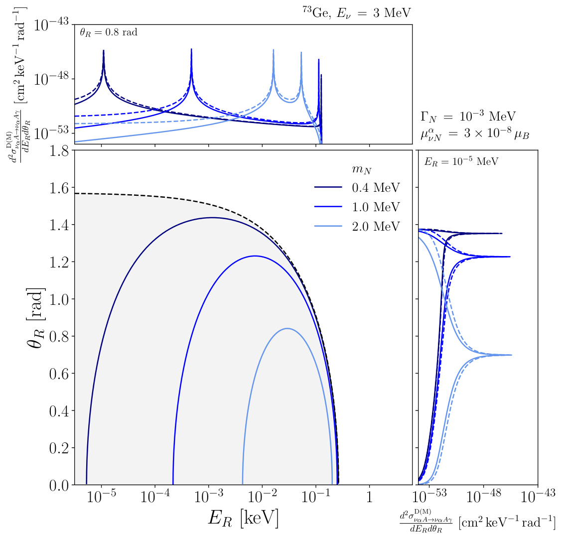
In Fig. 6 we depict the kinematically-allowed region as the grey shaded area in the main plot. The kinematically allowed region can be seen to be independent of the sterile neutrino mass . In the sub-plots above and to the right, we show the double differential cross section in Eq. (57) for fixed rad (above) and MeV (right) and three different values of . For illustrative purposes, we set the values of the transition magnetic moment and total decay width of to be and MeV, respectively. A total decay width of this size would require additional invisible decay modes of . We observe that, even though the double differential cross sections are non-zero over the entire kinematically allowed region, they are dominated by sharply peaked regions. This is a consequence of the total decay width of being much smaller than the mass of , justifying the use of the narrow width approximation (NWA).
In the limit, the following replacement can be made in Eq. (52),
| (61) |
which sets the intermediate to be on-shell, i.e. . Inserting the expression of in terms of the lab frame variables in Eq. (40) into allows to find the following relationship between the nuclear recoil angle and energy,
| (62) |
or equivalently,
| (63) |
where . In Fig. 6 we plot the curves of allowed values in the plane from the condition for three different values of . From the plots above and to the right, we see that the double differential cross section is sharply peaked at these values of and . For each value of there is an maximum recoil angle,
| (64) |
as well as minimum and maximum recoil energies given by Eq. (63) with . We now take Eqs. (54) and (55), make the substitution in Eq. (61) and integrate over by setting . To obtain the differential cross section in the nuclear recoil energy, we finally multiply by the Jacobian factor to obtain
| (65) |
In the NWA, the differential rate in the nuclear recoil for the process is therefore the Primakoff upscattering cross section multiplied by the branching ratio for the radiative decay .
To obtain the differential cross sections for in the outgoing photon energy and angle , we can instead integrate Eq. (52) over and as
| (66) |
where again the limits are found by solving for and by solving for . In general both integrals are non-trivial for the differential cross section in Eq. (52) because appears in the factor of in the denominator and appears in the nuclear form-factor ; it is therefore necessary to perform this integration numerically. Once this is done, it is possible to transform to the lab frame by multiplying Eq. (66) by the Jacobian . To obtain the single differential cross sections in the variables and , the remaining variables are integrated over as
| (67) | ||||
| (68) |
where the maximum allowed photon energy is .

However, the NWA can also be used to simplify the calculation above. The substitution in Eq. (61) can be made in Eq. (66) and the integration performed by setting . However, the integral must be still be performed numerically due to the non-trivial dependence of . Multiplying the double differential cross section by the Jacobian , we obtain the double differential cross section in and ,
| (69) |
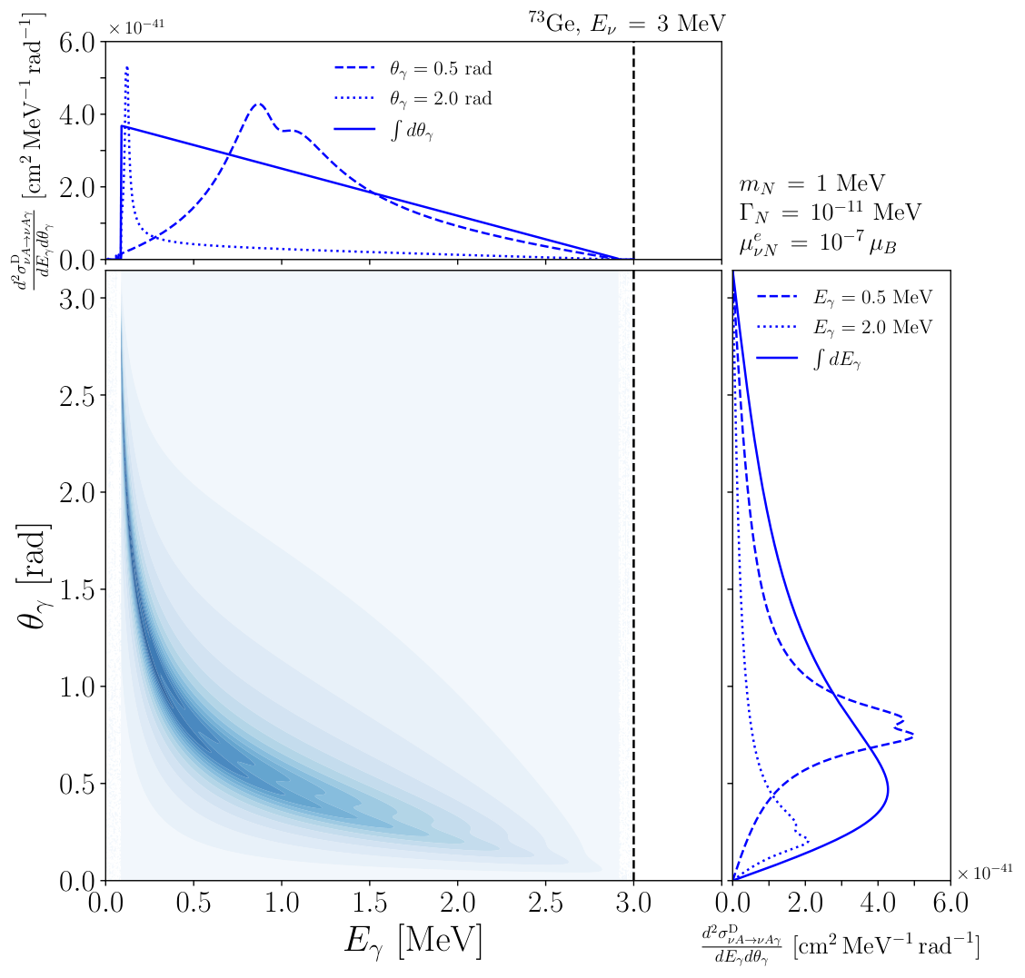
In the following, we set and perform the integral over analytically. In the NWA, the limits of integration can be found by solving for with . These limits correspond to the minimum and maximum photon energies
| (70) | ||||
| (71) |
For , these give the simple result .
In Fig. 7, we plot the double differential cross sections in and for Dirac (left) and Majorana (right) . We choose the values MeV, MeV and . In the sub-plots above and to the right of the contours, we also plot the double differential cross section for fixed values of the photon energy (right) and angle (above). Furthermore, we plot the single differential cross sections in and by integrating over the other variable as in Eqs. (67) and (68). Examining the single differential cross sections in the photon energy , we see a stark difference between the Dirac and Majorana cases. In the former case, the cross section decreases linearly with the energy, while in the latter the cross section is constant. The minimum and maximum photon energies in Eq. (70) can clearly be seen. Looking at the single differential cross sections in the photon angle , the difference between the Dirac and Majorana cases is less prominent; the Majorana cross section peaks at slightly lower angles compared to the Dirac cross section.
Differential rates: With the differential cross section for the Primakoff upscattering in Eq. (B), we can now calculate the differential rate of nuclear recoil events in a CENS experiment as
| (72) |
where is the flux of incoming neutrinos per cm2 per second and is the minimum incoming neutrino energy that can produce a sterile neutrino of mass and a nuclear recoil energy ,
| (73) |
In Eq. (72) we have divided by the mass number of the target isotope multiplied by the proton mass to determine the differential rate per unit mass of the target material.
Similarly, the differential rate for nuclear recoil events that are coincident with an outgoing photon in the detector is given (in the NWA) by
| (74) |
Here, we simply integrate over the flux multiplied by the radiative upscattering cross section and the probability for the decay to take place inside the detector. In the NWA, is again given by Eq. (73).
As an example, in Fig. 8 (left) we plot the differential Primakoff upscattering rate in the nuclear recoil energy for the NUCLEUS experiment situated at the very-near-site (VNS) of the Chooz reactor site, for MeV and . The flux of electron antineutrinos induces the process . In the plot we compare the rates for three different target materials; 73Ge (grey), (blue) and (orange). For and we average over the mass numbers of the constituent isotopes. We also compare the Primakoff upscattering rates to the SM CENS process (dotted lines). For , the number of Primakoff upscattering events is comparible the number of CENS events. The horizontal black dotted line indicates the predicted nuclear recoil background of 100 keV-1 kg-1 day-1 in the NUCLEUS detector at the VNS. The grey shaded region shows the range of nuclear recoils that can be detected by the experiment (i.e. a nuclear recoil threshold of 10 eV).
In Fig. 8 (right) we plot the differential rate in the nuclear recoil energy for the radiative upscattering process , again for the NUCLEUS experiment at the VNS and for MeV and . We assume that the outgoing antineutrino is of electron flavour, (i.e. there are no additional decay modes of ), and that the nuclear recoil is accompanied by an outgoing photon. We compare the cases where the intermediate sterile neutrino is a Dirac (solid lines) or Majorana (dashed lines) fermion, again for three different target materials.
One may first notice that there are peaks in these distributions, which otherwise have the same shape as the Primakoff upscattering distributions. The origin of these peaks is as follows; as we assume that can only decay radiatively, the branching ratio in the integrand of Eq. (74) is unity. For and cm, the total width satisfies and the decay probability can be Taylor expanded to give . The peaks occur at values of the nuclear recoil energy that minimise the minimum incoming neutrino energy in Eq. (73) and hence minimise . This in turn maximises and the integrand in Eq. (74). In other words, for these values of the nuclear recoil, the incoming neutrino energy is as close as possible to . The produced sterile state is non-relativistic and has a shorter decay length than average. If more decays occur inside the detector, we would expect to observe a peak in coincidence events.
It is also useful to obtain the differential rate for the radiative upscattering process in or as
| (75) |
where . In the NWA, the minimum incoming neutrino energy that can produce sterile neutrino of mass and a photon of energy is
| (76) |
For a given incoming neutrino energy and sterile neutrino mass , the outgoing photon can be emitted at any angle in the range . In the NWA, the minimum incoming neutrino energy is that which can produce a sterile neutrino of mass ,
| (77) |
In Fig. 9 we show the differential rates for the process in the outgoing photon energy (left) and photon angle (right) for a detector situated at the VNS of the Chooz reactor site. We again present the distributions for three target materials: 73Ge (grey), (blue) and (orange). For the Chooz reactor neutrino flux, the maximum number of events are expected for sterile neutrino masses MeV. We want to emphasise that the Dirac and Majorana cases (solid and dashed lines, respectively) have different distributions in the photon energy and angle. We again observe enhancements in Fig. 9 (left) at values of that minimise the minimum incoming neutrino energy, i.e. .
References
- Freedman (1974) D. Z. Freedman, Phys. Rev. D 9, 1389 (1974).
- Akimov et al. (2017) D. Akimov et al. (COHERENT), Science 357, 1123 (2017), arXiv:1708.01294 [nucl-ex] .
- Rothe et al. (2019) J. Rothe et al. (NUCLEUS), J. Low Temp. Phys. 199, 433 (2019).
- Angloher et al. (2019) G. Angloher et al. (NUCLEUS), Eur. Phys. J. C 79, 1018 (2019), arXiv:1905.10258 [physics.ins-det] .
- Schwetz et al. (2020) T. Schwetz, A. Zhou, and J.-Y. Zhu, JHEP 21, 200 (2020), arXiv:2105.09699 [hep-ph] .
- Coloma et al. (2017) P. Coloma, P. A. N. Machado, I. Martinez-Soler, and I. M. Shoemaker, Phys. Rev. Lett. 119, 201804 (2017), arXiv:1707.08573 [hep-ph] .
- Atkinson et al. (2022) M. Atkinson, P. Coloma, I. Martinez-Soler, N. Rocco, and I. M. Shoemaker, JHEP 04, 174 (2022), arXiv:2105.09357 [hep-ph] .
- Voloshin (1988) M. B. Voloshin, Sov. J. Nucl. Phys. 48, 512 (1988).
- Pal and Wolfenstein (1982) P. B. Pal and L. Wolfenstein, Phys. Rev. D 25, 766 (1982).
- Shrock (1982) R. E. Shrock, Nucl. Phys. B 206, 359 (1982).
- Bell et al. (2005) N. F. Bell, V. Cirigliano, M. J. Ramsey-Musolf, P. Vogel, and M. B. Wise, Phys. Rev. Lett. 95, 151802 (2005), arXiv:hep-ph/0504134 .
- Cepedello et al. (2019) R. Cepedello, F. F. Deppisch, L. González, C. Hati, and M. Hirsch, Phys. Rev. Lett. 122, 181801 (2019), arXiv:1811.00031 [hep-ph] .
- Magill et al. (2018) G. Magill, R. Plestid, M. Pospelov, and Y.-D. Tsai, Phys. Rev. D 98, 115015 (2018), arXiv:1803.03262 [hep-ph] .
- Bolton et al. (2019) P. D. Bolton, F. F. Deppisch, C. Hati, S. Patra, and U. Sarkar, Phys. Rev. D 100, 035013 (2019), arXiv:1902.05802 [hep-ph] .
- Brdar et al. (2021) V. Brdar, A. Greljo, J. Kopp, and T. Opferkuch, JCAP 01, 039 (2021), arXiv:2007.15563 [hep-ph] .
- Babu et al. (2020) K. S. Babu, S. Jana, and M. Lindner, JHEP 10, 040 (2020), arXiv:2007.04291 [hep-ph] .
- Kayser and Shrock (1982) B. Kayser and R. E. Shrock, Phys. Lett. B 112, 137 (1982).
- Kayser (1982) B. Kayser, Phys. Rev. D 26, 1662 (1982).
- Vogel and Engel (1989) P. Vogel and J. Engel, Phys. Rev. D 39, 3378 (1989).
- Balantekin and Vassh (2014) A. B. Balantekin and N. Vassh, Phys. Rev. D 89, 073013 (2014), arXiv:1312.6858 [hep-ph] .
- Strauss et al. (2021) R. Strauss et al. (NUCLEUS), (2021), Private Communication .
- Giunti and Studenikin (2015) C. Giunti and A. Studenikin, Rev. Mod. Phys. 87, 531 (2015), arXiv:1403.6344 [hep-ph] .
- Li et al. (2020) T. Li, X.-D. Ma, and M. A. Schmidt, JHEP 07, 152 (2020), arXiv:2005.01543 [hep-ph] .
- Li and Wilczek (1982) L. F. Li and F. Wilczek, Phys. Rev. D 25, 143 (1982).
- Baha Balantekin and Kayser (2018) A. Baha Balantekin and B. Kayser, Ann. Rev. Nucl. Part. Sci. 68, 313 (2018), arXiv:1805.00922 [hep-ph] .
- Balantekin et al. (2019) A. B. Balantekin, A. de Gouvêa, and B. Kayser, Phys. Lett. B 789, 488 (2019), arXiv:1808.10518 [hep-ph] .
- Balaji et al. (2020a) S. Balaji, M. Ramirez-Quezada, and Y.-L. Zhou, JHEP 04, 178 (2020a), arXiv:1910.08558 [hep-ph] .
- Balaji et al. (2020b) S. Balaji, M. Ramirez-Quezada, and Y.-L. Zhou, JHEP 12, 090 (2020b), arXiv:2008.12795 [hep-ph] .
- de Gouvea et al. (2021) A. de Gouvea, P. J. Fox, B. J. Kayser, and K. J. Kelly, Phys. Rev. D 104, 015038 (2021), arXiv:2104.05719 [hep-ph] .
- (30) P. D. Bolton, F. F. Deppisch, K. Fridell, J. Harz, C. Hati, and S. Kulkarni, In preparation .
- Plestid (2021) R. Plestid, Phys. Rev. D 104, 075027 (2021), arXiv:2010.04193 [hep-ph] .
- Shoemaker and Wyenberg (2019) I. M. Shoemaker and J. Wyenberg, Phys. Rev. D 99, 075010 (2019), arXiv:1811.12435 [hep-ph] .
- Dasgupta et al. (2021) A. Dasgupta, S. K. Kang, and J. E. Kim, JHEP 11, 120 (2021), arXiv:2108.12998 [hep-ph] .
- Gninenko and Krasnikov (1999) S. N. Gninenko and N. V. Krasnikov, Phys. Lett. B 450, 165 (1999), arXiv:hep-ph/9808370 .
- Miranda et al. (2021) O. G. Miranda, D. K. Papoulias, O. Sanders, M. Tórtola, and J. W. F. Valle, JHEP 12, 191 (2021), arXiv:2109.09545 [hep-ph] .
- Mohapatra (1986) R. N. Mohapatra, Phys. Rev. Lett. 56, 561 (1986).
- Mohapatra and Valle (1986) R. N. Mohapatra and J. W. F. Valle, Phys. Rev. D 34, 1642 (1986).
- Gonzalez-Garcia and Valle (1989) M. C. Gonzalez-Garcia and J. W. F. Valle, Phys. Lett. B 216, 360 (1989).
- Byckling and Kajantie (1971) E. Byckling and K. Kajantie, Particle Kinematics: (Chapters I-VI, X) (University of Jyvaskyla, Jyvaskyla, Finland, 1971).