The generalized Floquet-Bloch spectrum
for periodic thermodiffusive layered materials

In the last years, composite laminates subject to thermodiffusive phenomena have been largely used in the design and fabrication of renewable energy devices characterized by a multi-layered configuration, such as lithium-ion batteries (Ellis et al. 2012; Salvadori et al. 2014), solid oxide fuel cells (SOFCs) (Kakac et al. 2007; Colpan et al. 2008; Kim et al. 2009; Kuebler et al. 2010; Hasanov et al. 2011; Nakajo et al. 2012; Dev et al. 2014) and photovoltaic modules (PV) (Paggi et al. 2013). Several studies (Atkinson and Sun 2007; Delette et al. 2013) have shown that, in real operative scenarios, performances in terms of power generation and energy conversion efficiency can be compromised because of the severe thermomechanical stress as well as intense particle flows to which components of such energy devices are subjected (Muramatsu et al. 2015). This can ultimately impact on their resistance to damage with resulting cracks formation and spreading. Consequently, modeling and predicting these phenomena is a crucial issue in order to ensure the successful manufacture of multi-layered renewable energy devices and to optimize their performances. Energy devices of this kind are generally organized in stacks where more elements are separated by metallic interconnections (Molla et al. 2016). Due to their particular structure, they can be modelled as periodic themodiffusive laminates which elementary cell, representing the single device, is composed of an arbitrary number of elasto-themodiffusive phases. This idealised representation provides the possibility of estimating the overall mechanical and thermodiffusive properties of such multi-layered systems through homogenization methods, avoiding the challenging computations required by the direct numerical study of the heterogeneous structures (Bove and Ubertini 2008; Richardson et al. 2012; Hajimolana et al. 2011). Homogenization techniques, in fact, allow to take into account the role of the microstructure upon the overall constitutive behaviour of composite materials in a concise, but accurate way. They have been a matter of extremely intensive research within the last decades and, in a general sense, homogenization procedures can be classified in asymptotic techniques (Bakhvalov and Panasenko 1984) togheter with their extension to multi-field phenomena (Fantoni et al. 2017; Fantoni et al. 2018; Fantoni et al. 2019), variational-asymptotic techniques (Smyshlyaev and Cherednichenko 2000), and different identification approaches, involving the analytical (Bigoni and Drugan 2007; Bacca et al. 2013a; Bacca et al. 2013b) and computational techniques (Forest 2002; Lew et al. 2004; Scarpa et al. 2009; De Bellis and Addessi 2011; Forest and Trinh 2011; Wang et al. 2017; Yvonnet et al. 2020). Furthermore, dynamic homogenization schemes, useful to approximate frequency band structure of periodic media at high frequencies, can be found in (Zhikov 2000; Smyshlyaev 2009; Craster et al. 2010; Bacigalupo and Lepidi 2016; Sridhar et al. 2018; Kamotski and Smyshlyaev 2019; Bacigalupo and Gambarotta 2019). In the context of multi-field asymptotic homogenization methods applied to thermodiffusive phenomena, Bacigalupo et al. 2016a; Bacigalupo et al. 2016b investigated the static overall constitutive properties of periodic media. The dynamics of periodic thermodiffusive devices has been subsequently investigated via asymptotic homogenization in Fantoni and Bacigalupo 2020. The dynamic behaviour of laminate media with microstructure has been extensively studied (Qian et al. 2004; Willis 2009; Nemat-Nasser and Srivastava 2011; Caviglia and Morro 2012). In the context of energy devices, the interest is motivated by the fact that media are subject to intrinsically dynamic phenomena such as shock thermal waves, interface waves and instabilities which cannot be described in the framework of static, quasi-static or steady-state formulations. In this regard, an accurate analysis of the harmonic waves propagation in thermodiffusive laminate media, and especially of the effects of the coupling between mechanical, thermal and diffusive observables, has not been addressed in details to the authors knowledge. Indeed, most of the work conducted on this topics have been performed adopting the generalized theories of thermoelasticity and thermodiffusion (Lord and Shulman 1967; Sherief et al. 2004). These approaches provide thermal and diffusive relaxation times and then the standard heat and mass conduction equations are transformed in hyperbolic type equations. In doing so, both the temperature and the mass fields evolve in the medium in form of heat and diffusive waves having finite propagation speeds which interact with the mechanical waves. In contrast, we propose a different formulation assuming that the elastic waves equation is coupled with the standard heat conduction and mass diffusion equations. These lasts are of parabolic type and are then associated with an imaginary part of the spectrum corresponding to damping phenomena. We implement the generalized Floquet-Bloch quasiperiodic conditions, and by means of a generalization of the transfer matrix method (Hawwa and Nayfeh 1995), we derive a general expression for the characteristic equation valid for periodic thermodiffusive laminates which elementary cell is composed by an arbitrary number of phases. The transfer matrix method has been widely exploited in order to investigate waves propagation in periodic media (Adams et al. 2008; Shmuel and Band 2016; Lee and Lee 2017; Wang et al. 2018). Symplecticity properties of the transfer matrix to which corresponds a palindromic characteristic polynomial are exploited in order to solve the eigenvalues problem associated with the characteristic equation, and this general procedure provides the frequency band structure (complex spectra) associated to wave propagating inside the medium. The potentialities of this technique are illustrated through illustrative examples where the propagation and damping of harmonic thermal and diffusive oscillations as well as of mechanical waves in bi-phase laminates of interest for SOFCs realization is addressed. The observed damping effects are due to the imaginary part of the spectra, which derives from the parabolicity of heat conduction and mass transfer equations. Therefore, these phenomena cannot be detected by means of the other approaches currently available in the literature, based on hyperbolic equations. The paper is organized as follows: Section 2 summarizes governing equations for a linear thermodiffusive material and the wave-like expression of harmonic plane oscillations propagating inside the medium. Section 3 is dedicated to present the generalization of the transfer matrix method exploited to obtain, together with Floquet-Bloch conditions, complex spectra for thermodiffusive laminates. Representative examples are performed in Section 4, thus showing complex spectra obtained for bi-phase isotropic thermodiffusive laminates of interest for SOFCs fabrication in order to investigate the effects of thermodiffusive coupling upon propagation and damping properties of elastic waves traveling inside the composite. Finally, conclusions are addressed in Section 5.

One considers a plane thermodiffusive laminate medium whose periodic cell is composed by an arbitrary number of layers $n$ perfectly bonded at their interfaces and stacked along the $x_{2}-$axis (see figure 1 ). Each material point is identified by the position vector $\mbox{\boldmath$x$}=x_{1}\mbox{\boldmath$e$}_{1}+x_{2}\mbox{\boldmath$e$}_{2}$ referred to a system of coordinates with origin at point $O$ and orthogonal base $[\mbox{\boldmath$e$}_{1},\mbox{\boldmath$e$}_{2}]$. The periodic cell $\mathcal{A}$ has a characteristic length equal to $L$ in the direction perpendicular to material layering and it is translationally invariant along the layering. As depicted in figure 1-(b), $L=\sum_{m=1}^{n}\ell_{m}$ where $\ell_{m}$ represents the thickness of each single layer. In the followings, governing equations for a linear thermodiffusive material are introduced.

Introducing the eight-components vector $\mathbf{r}=(\mathbf{w}^{{}^{\prime}}\,\,\mathbf{w})^{T}$, one can easily transform the second order $4\times 4$ system (22) in the following equivalent first order $8\times 8$ system

$$\mathbf{M}\mathbf{r}^{{}^{\prime}}+\mathbf{N}\mathbf{r}=\mathbf{0},$$

(51)

where $\mathbf{M}$ is a non singular square diagonal block matrix and $\mathbf{N}$ is a square block matrix. They are $8\times 8$ matrices expressed, respectively, as

$$\mathbf{M}=\left(\begin{array}[]{cc}\mathbf{A}&\mathbf{0}\\ \mathbf{0}&\mathbf{I}\end{array}\right),\quad\mathbf{N}=\left(\begin{array}[]{cc}\mathbf{B}&\mathbf{C}\\ -\mathbf{I}&\mathbf{0}\end{array}\right).$$

(52)

General solution of first order ordinary differential system (51) can be written as

$$\mathbf{r}=\textrm{exp}\left[\mathbf{M}^{-1}\mathbf{N}x_{2}\right]\,\mathbf{c},$$

(53)

where $\mathbf{c}$ is a vector of constants and $\textrm{exp}[\,\cdot\,]$ denotes the matrix exponential. A possible procedure to compute matrix exponential is detailed in Appendix A. Denoting with $\mathbf{y}(x_{1},x_{2},t)$ a vector containing the components of solution vector $\mathbf{v}(x_{1},x_{2},t)$ of equation (13) and of the generalized traction vector $\mathbf{s}(x_{1},x_{2},t)$ defined as

$$\mathbf{s}(x_{1},x_{2},t)=(\sigma_{21}\,\,\sigma_{22}\,\,q_{2}\,\,j_{2})^{T}=\mathbf{t}(x_{2})\,\textrm{exp}\left[i\left(\mathbf{k}\cdot\mathbf{x}-\omega t\right)\right],$$

(54)

where $\mathbf{t}$ is given by

$$\mathbf{t}(x_{2})=\left(\tilde{\sigma}_{21}(x_{2})\,\,\ \tilde{\sigma}_{22}(x_{2})\,\,\ \tilde{q}_{2}(x_{2})\,\,\ \tilde{j}_{2}(x_{2})\right)^{T},$$

(55)

it can be expressed in terms of $\mathbf{r}$ in the following way

$$\mathbf{y}(x_{1},x_{2},t)=\left(\begin{array}[]{c}\mathbf{v}(x_{1},x_{2},t)\\ \mathbf{s}(x_{1},x_{2},t)\end{array}\right)=\textrm{exp}\left[i(\mathbf{k}\cdot\mathbf{x}-\omega t)\right]\left(\begin{array}[]{c c}\mathbf{0}&\mathbf{I}\\ \mathbf{R}&i\mathbf{R}k_{2}+\mathbf{S}\end{array}\right)\,\mathbf{r},$$

(56)

where $\mathbf{I}$ is a $4\times 4$ identity operator and non singular diagonal matrix $\mathbf{R}$ and coupling singular matrix $\mathbf{S}$ are expressed, respectively, as

$$\mathbf{R}=\left(\begin{array}[]{c c c c }C_{1212}&0&0&0\\ 0&C_{2222}&0&0\\ 0&0&-K_{22}&0\\ 0&0&0&-D_{22}\end{array}\right),\hskip 14.22636pt\mathbf{S}=\left(\begin{array}[]{c c c c }0&0&0&0\\ 0&0&-\alpha_{22}&-\beta_{22}\\ 0&0&0&0\\ 0&0&0&0\end{array}\right).$$

(57)

Plugging solution (53) into (56) one obtains

$$\mathbf{y}(x_{1},x_{2},t)=\left(\begin{array}[]{c c}\mathbf{0}&\mathbf{I}\\ \mathbf{R}&i\mathbf{R}k_{2}+\mathbf{S}\end{array}\right)\textrm{exp}\left[-\mathbf{M}^{-1}\mathbf{N}x_{2}\right]\mathbf{c}\,\textrm{exp}\left[i(\mathbf{k}\cdot\mathbf{x}-\omega t)\right].$$

(58)

If the single $m^{th}$ layer belonging to the periodic cell shown in figure 1 has thickness $\ell_{m}$, referring to a local coordinate system as the one depicted in figure 2, such as along the $x_{2}-$axis the layer extends in the range $-\ell_{m}/2\leq x_{2}\leq\ell_{m}/2$, one can define the generalized vector $\mathbf{y}$ containing displacement components, relative temperature, relative chemical potential, tractions, heat and mass fluxes at the upper and lower boundaries of the layer as

	$\displaystyle\mathbf{y}_{m}^{+}$	$\displaystyle=$	$\displaystyle\mathbf{y}_{m}(x_{1},x_{2}=\ell_{m}/2,t)=\left(\begin{array}[]{c c}\mathbf{0}&\mathbf{I}\\ \mathbf{R}&i\mathbf{R}k_{2}+\mathbf{S}\end{array}\right)\textrm{exp}\left[-\mathbf{M}^{-1}\mathbf{N}\ell_{m}/2\right]\mathbf{c}\,\,\textrm{exp}\left[i(k_{1}x_{1}+k_{2}\ell_{m}/2-\omega t)\right],$
	$\displaystyle\mathbf{y}_{m}^{-}$	$\displaystyle=$	$\displaystyle\mathbf{y}_{m}(x_{1},x_{2}=-\ell_{m}/2,t)=\left(\begin{array}[]{c c}\mathbf{0}&\mathbf{I}\\ \mathbf{R}&i\mathbf{R}k_{2}+\mathbf{S}\end{array}\right)\textrm{exp}\left[\mathbf{M}^{-1}\mathbf{N}\ell_{m}/2\right]\mathbf{c}\,\,\textrm{exp}\left[i(k_{1}x_{1}-k_{2}\ell_{m}/2-\omega t)\right].$

Since block matrix premultiplying the exponential matrix is non singular by definition, from equation () constants vector $\mathbf{c}$ gains the form

$$\mathbf{c}=\textrm{exp}\left[-\mathbf{M}^{-1}\mathbf{N}\ell_{m}/2\right]\left(\begin{array}[]{c c}\mathbf{0}&\mathbf{I}\\ \mathbf{R}&i\mathbf{R}k_{2}+\mathbf{S}\end{array}\right)^{-1}\mathbf{y}^{-}_{m}\,\textrm{exp}\left[i(k_{1}x_{1}-k_{2}\ell_{m}/2-\omega t)\right].$$

(67)

Substitution of expression (67) into (3) leads to express $\mathbf{y}_{m}^{+}$ in terms of $\mathbf{y}_{m}^{-}$ as

$$\mathbf{y}_{m}^{+}=\left(\begin{array}[]{c c}\mathbf{0}&\mathbf{I}\\ \mathbf{R}&i\mathbf{R}k_{2}+\mathbf{S}\end{array}\right)\textrm{exp}\left[-\mathbf{M}^{-1}\mathbf{N}\ell_{m}\right]\left(\begin{array}[]{c c}\mathbf{0}&\mathbf{I}\\ \mathbf{R}&i\mathbf{R}k_{2}+\mathbf{S}\end{array}\right)^{-1}\,\textrm{exp}\left[{ik_{2}\ell_{m}}\right]\mathbf{y}_{m}^{-}=\mathbf{T_{m}}\,\mathbf{y}_{m}^{-},$$

(68)

where $\mathbf{T}_{m}$ is the frequency-dependent transfer matrix of the $m^{th}$ thermodiffusive elastic layer (Gupta 1970; Faulkner and Hong 1985). Since relation (68) is valid for each single layer forming the periodic cell and since it is assumed that the layers are perfectly bonded, so that continuity condition

$$\mathbf{y}^{+}_{m}=\mathbf{y}^{-}_{m+1}$$

(69)

must be satisfied at the interface between two subsequent layers $m$ and $m+1$ (see figure 2), the following equation can be easily derived relating generalized vector at the upper boundary of the last $n^{th}$ layer $\mathbf{y}_{n}^{+}$ to the generalized vector at the lower boundary of the first layer $\mathbf{y}_{1}^{-}$. It reads

$$\mathbf{y}_{n}^{+}=\mathbf{T}_{(1,n)}\,\mathbf{y}_{1}^{-},$$

(70)

where $\mathbf{T}_{(1,n)}=\prod_{i=0}^{n-1}\mathbf{T}_{n-i}$ is the frequency-dependent transfer matrix of the entire periodic cell.

In virtue of the periodicity of cell $\mathcal{A}$, the following Floquet-Bloch boundary condition (Floquet 1883; Bloch 1929; Brillouin 1953; Mead 1973; Langley 1993) can be imposed

$$\mathbf{y}^{+}_{n}=\textrm{exp}\left[ik_{2}L\right]\mathbf{y}^{-}_{1},$$

(71)

where, due to the geometry of the system (see figure 1), the periodicity direction is assumed to be along the $x_{2}-$axis and, as already mentioned, $L=\sum_{m=1}^{n}\ell_{m}$ is the extent of the whole periodic cell along that direction. Substituting (71) into (70), one obtains the following standard eigenvalue problem

$$\left(\mathbf{T}_{(1,n)}-\lambda\mathbf{I}\right)\mathbf{y}_{1}^{-}=\mathbf{0},$$

(72)

where $\lambda=\textrm{exp}\left[ik_{2}L\right]$ is called Floquet multiplier and $\mathbf{I}$ represents an $8\times 8$ identity operator. The system (72) admits a non-trivial solution when the following characteristic equation is satisfied

$$\mathcal{D}(\mathbf{k},\omega)=\textrm{Det}\left(\mathbf{T}_{(1,n)}-\lambda\mathbf{I}\right)=0.$$

(73)

Equation (73) is the dispersion relation of plane oscillations in periodic thermodiffusive laminates where the elementary cell is composed by an arbitrary number of layers $n$. Furthermore, transfer matrix $\mathbf{T}_{(1,n)}$ results to be a symplectic matrix having a unitary determinant. In the most general case, both the wave vector $\mathbf{k}$ and the angular frequency $\omega$, to which characteristic equation $\mathcal{D}$ depends, can be complex, namely $\mathbf{k}=(k_{1r}+i\,k_{1i})\mathbf{e}_{1}+(k_{2r}+i\,k_{2i})\mathbf{e}_{2}$ and $\omega=\omega_{r}+i\,\omega_{i}$. In this case, wave vector $\mathbf{k}$ can be specialized in the form

$$\mathbf{k}=\mathbf{k}_{r}+i\mathbf{k_{i}}=k_{r}\,\mathbf{n}_{r}+i\,k_{i}\,\mathbf{n}_{i},$$

(74)

where $\mathbf{k}_{r}$ represents the real wave vector having magnitude $k_{r}$ and direction $\mathbf{n}_{r}\in\mathbb{R}^{2}$, and $\mathbf{k}_{i}$ is the attenuation vector with magnitude $k_{i}$ and direction $\mathbf{n}_{i}\in\mathbb{R}^{2}$. A plane wave can be defined as homogeneous when the direction of normals to planes of constant phase $\mathbf{n}_{r}$ coincides with the one of normals to planes of constant amplitude $\mathbf{n}_{i}$, namely when $\mathbf{n}_{r}\times\mathbf{n}_{i}=\mathbf{0}$ (Carcione 2007). Denoting with $\mathbf{n}$ such a direction one has

$$\mathbf{k}=\left(k_{r}+i\,k_{i}\right)\mathbf{n}=\kappa\,\mathbf{n},$$

(75)

with $\kappa$ the complex wave number. Furthermore, being $\mathbf{k}_{r}/k_{r}=\mathbf{k}_{i}/k_{i}$, for an homogeneous wave one obtains the following relation among the real and imaginary parts of $k_{1}$ and $k_{2}$

$$k_{1r}\,k_{2i}=k_{2r}\,k_{1i}.$$

(76)

When $\mathbf{k}\in\mathbb{C}^{2}$ and $\omega\in\mathbb{C}$, frequency spectrum is determined from the intersection of two hypersurfaces immersed in a space in $\mathbb{R}^{6}$, representing respectively the vanishing of the real and imaginary part of characteristic equation (73), namely

$$\left\{\begin{array}[]{l}\textrm{Re}\left(\mathcal{D}\left(k_{1r},k_{1i},k_{2r},k_{2i},\omega_{r},\omega_{i}\right))\right)=0\\ \textrm{Im}\left(\mathcal{D}\left(k_{1r},k_{1i},k_{2r},k_{2i},\omega_{r},\omega_{i}\right)\right)=0\end{array}\right..$$

(77)

In order to investigate spatial damping for the material at hand, the wave vector $\mathbf{k}$ is considered as complex ($k_{\alpha}=k_{\alpha r}+i\,k_{\alpha i}$ with $\alpha=1,2$) and the angular frequency $\omega$ as real (Caviglia and Morro 1992). In the particular case where the value of one component $k_{\alpha}$ is fixed ($\alpha=1$ or $\alpha=2$), frequency spectrum is obtained through the intersection of two surfaces in $\mathbb{R}^{3}$, namely the plane $\{k_{\beta r},k_{\beta i},\omega\}$, with $\beta\neq\alpha$, as

$$\left\{\begin{array}[]{l}\textrm{Re}(\mathcal{D}(k_{\beta r},k_{\beta i},\omega))=0\\ \textrm{Im}(\mathcal{D}(k_{\beta r},k_{\beta i},\omega))=0\\ \end{array}\right.,$$

(78)

and, if fixing $k_{\alpha}$ equation (76) results satisfied, the plane wave is homogeneous. By fixing, for example, component $k_{1}$ of complex wave vector $\mathbf{k}$, a procedure for obtaining material frequency band structure that is alternative to (78) is to directly solve linear eigenvalue problem (72), where the Floquet multiplier $\lambda$ is the eigenvalue and $\mathbf{y}_{1}^{-}$ is the eigenvector. In this situation, in fact, it is possible to prove that transfer matrix $\mathbf{T}_{(1,n)}$ results to be independent upon $k_{2}$ and characteristic equation (73) reduces to the $8^{th}$-degree associated polynomial. In this case, being the wave number related to the Floquet multiplier by relation $k_{2}=\textrm{ln}(\lambda)/(i\,L)$, its real and imaginary parts are expressed in terms of $\lambda=\lambda_{r}+i\,\lambda_{i}$ as

$$k_{2r}=\frac{\textrm{Arg}(\lambda_{r}+i\,\lambda_{i})}{L},\hskip 14.22636ptk_{2i}=-\frac{1}{2}\frac{\textrm{ln}(\lambda_{r}^{2}+\lambda_{i}^{2})}{L},$$

(79)

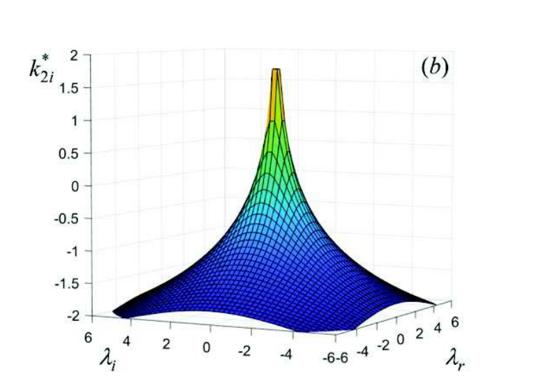
where symbol $\textrm{Arg}(\cdot)$ denotes the argument of a complex number. As expected, $k_{2r}L$ is a function whose values belong to the first, dimensionless, Brillouin zone $(-\pi,\pi]$. Figure 3 shows the behaviour of dimensionless wave numbers $k_{2r}^{*}=k_{2r}L$ and $k_{2i}^{*}=k_{2i}L$ in terms of the real and imaginary parts of Floquet multiplier $\lambda$. As depicted in figure 3-(a), $k_{2r}^{*}$ shows a branch cut discontinuity in the complex $\lambda$ plane running from $-\infty$ to $0$.

Moreover, since $\mathbf{T}_{(1,n)}$ is a symplectic matrix, if $\lambda_{k}$ is the $k^{th}$ eigenvalue for characteristic equation (73), also $1/\lambda_{k}$ is an eigenvalue. Such eigenvalues, in fact, are the roots of a palindromic characteristic polynomial, which is characterized by a reduced number of invariants (Hennig and Tsironis 1999; Romeo and Luongo 2002; Bronski and Rapti 2005; Xiao et al. 2013; Carta and Brun 2015; Carta et al. 2016). A procedure to compute the invariants of such characteristic polynomial is detailed in Appendix B. When component $k_{2}$ of $\mathbf{k}$ is fixed, in order to study wave propagation in the $\mathbf{e}_{1}$ direction, one could exploit the formal solution outlined in Appendix C, which allows expressing transfer matrix $\mathbf{T}_{m}$ of the single $m^{th}$ layer as a power series of wave number $k_{1}$. In this way, by combining transfer matrices of all the $n$ layers constituting the periodic cell, one obtains the transfer matrix of the entire cell $\mathbf{T}_{(1,n)}$ as a power series of $k_{1}$. Truncating this last at a proper order, it is possible to obtain an approximation of the eigenvalue problem (73) showing a polynomial dependence upon $k_{1}$, which can be used to investigate propagation of plane waves in the $\mathbf{e}_{1}$ direction. Temporal damping is studied by considering the angular frequency $\omega$ in (73) as complex ($\omega=\omega_{r}+i\,\omega_{i}$) and wave vector $\mathbf{k}$ as real (Carcione 2007). In this case, once a component of $\mathbf{k}$ is fixed ($k_{\alpha}$ with $\alpha=1$ or $2$), frequency spectrum is obtained by means of the intersection between two surfaces in $\mathbb{R}^{3}$, namely the plane $\{k_{\beta},\omega_{r},\omega_{i}\}$, with $\beta\neq\alpha$. Such surfaces represent the vanishing of the real and imaginary parts of implicit function $\mathcal{D}$, namely

$$\left\{\begin{array}[]{l}\textrm{Re}(\mathcal{D}(k_{\beta},\omega_{r},\omega_{i}))=0\\ \textrm{Im}(\mathcal{D}(k_{\beta},\omega_{r},\omega_{i}))=0\\ \end{array}\right..$$

(80)

Analogously to what done for spatial damping, Appendix D describes a formal procedure to express transfer matrix of a single layer as a power series of angular frequency $\omega$. Following the same path of reasoning as before, transfer matrix of the entire periodic cell can thus be truncated at a proper order of $\omega$ in order to obtain a useful approximation of the eigenvalue problem (73) with a polynomial dependence upon $\omega$ with the aim of investigating temporal damping for the material at hand.

Solution of the general characteristic equation (73) is performed in the followings for thermodiffusive multi-layered systems of interest for engineering and technology applications. In particular, the behaviour of a thermodiffusive bi-layered composite which can be used in the fabrication of solid oxide fuel cells (SOFCs) (Bacigalupo et al. 2014; Bacigalupo et al. 2016b; Fantoni and Bacigalupo 2020), is explored. Focusing the attention upon spatial damping inside the system, the linear eigenvalue problem (72) has been solved in terms of the Floquet multiplier $\lambda$. Referring to coordinate system represented in figure 2, for a fixed value of $k_{1}$, the behaviour of real and imaginary parts of $k_{2}$, related, respectively, to the propagating part and to the spatial attenuation of the wave, is investigated with respect to the real independent parameter $\omega$. By means of a parametric analysis, the effects of the coupling between thermal, diffusive and mechanical fields on the dispersion and damping curves as well as their physical implications are discussed in details.

References

- Adams et al. (2008) Adams, S.D., Craster, R.V., Guenneau, S., 2008. Bloch waves in periodic multi-layered acoustic waveguides. Proceedings of the Royal Society A: Mathematical, Physical and Engineering Sciences 464, 2669–2692.
- Anandakumar et al. (2010) Anandakumar, G., Li, N., Verma, A., Singh, P., Kim, J.H., 2010. Thermal stress and probability of failure analyses of functionally graded solid oxide fuel cells. J. Power Sources 195, 6659–6670.
- Arfken and Weber (2005) Arfken, G.B., Weber, H.J., 2005. Mathematical methods for physicists, 5th edition. Elsevier Academic Press, San Diego.
- Atkinson and Sun (2007) Atkinson, A., Sun, B., 2007. Residual stress and thermal cycling of planar solid oxide fuel cells. Mater. Sci. Tech. 23, 1135–1143.
- Bacca et al. (2013a) Bacca, M., Bigoni, D., Dal Corso, F., Veber, D., 2013a. Mindlin second-gradient elastic properties from dilute two-phase Cauchy-elastic composites. Part I: closed form expression for the effective higher-order constitutive tensor. Int. J. Solids Struct. 50, 4010–4019.
- Bacca et al. (2013b) Bacca, M., Bigoni, D., Dal Corso, F., Veber, D., 2013b. Mindlin second-gradient elastic properties from dilute two-phase Cauchy-elastic composites. Part II: higher-order constitutive properties and application cases. Int. J. Solids Struct. 50, 4020–4029.
- Bacigalupo and Gambarotta (2019) Bacigalupo, A., Gambarotta, L., 2019. Generalized micropolar continualization of 1d beam lattices. International Journal of Mechanical Sciences 155, 554–570.
- Bacigalupo and Lepidi (2016) Bacigalupo, A., Lepidi, M., 2016. High-frequency parametric approximation of the floquet-bloch spectrum for anti-tetrachiral materials. International Journal of Solids and Structures 97, 575–592.
- Bacigalupo et al. (2014) Bacigalupo, A., Morini, L., Piccolroaz, A., 2014. Effective elastic properties of planar SOFCs: a non-local dynamic homogenization approach. Int. J. Hydrogen Energy 39, 15017–15030.
- Bacigalupo et al. (2016a) Bacigalupo, A., Morini, L., Piccolroaz, A., 2016a. Multiscale asymptotic homogenization analysis of thermo-diffusive composite materials. Int. J. Solids Struct. 85-86, 15–33.
- Bacigalupo et al. (2016b) Bacigalupo, A., Morini, L., Piccolroaz, A., 2016b. Overall thermomechanical properties of layered materials for energy devices applications. Comp. Struct. 157, 366–385.
- Bakhvalov and Panasenko (1984) Bakhvalov, N.S., Panasenko, G.P., 1984. Homogenization: averaging processes in periodic media. Kluwer Academic Publishers, Dordrecht-Boston-London.
- Bigoni and Drugan (2007) Bigoni, D., Drugan, W.J., 2007. Analytical derivation of Cosserat moduli via homogenization of heterogeneous elastic materials. ASME J. Appl. Mech. 74, 741–753.
- Bloch (1929) Bloch, F., 1929. Über die quantenmechanik der elektronen in kristallgittern. Zeitschrift für physik 52, 555–600.
- Bove and Ubertini (2008) Bove, R., Ubertini, S., 2008. Modeling solid oxide fuel cells: methods, procedures and techniques. Springer, Netherlands.
- Brandon and Brett (2006) Brandon, N.P., Brett, D.J., 2006. Engineering porous materials for fuel cell applications. Phil. Trans. R. Soc. A 364, 147–159.
- Brillouin (1953) Brillouin, L., 1953. Wave propagation in periodic structures: electric filters and crystal lattices .
- Bronski and Rapti (2005) Bronski, J.C., Rapti, Z., 2005. Modulational instability for nonlinear schrödinger equations with a periodic potential. Dynamics of Partial Differential Equations 2, 335–355.
- Carcione (2007) Carcione, J., 2007. Wave fields in real media: Wave propagation in anisotropic, anelastic, porous and electromagnetic media. Elsevier.
- Carta and Brun (2015) Carta, G., Brun, M., 2015. Bloch–floquet waves in flexural systems with continuous and discrete elements. Mechanics of Materials 87, 11–26.
- Carta et al. (2016) Carta, G., Brun, M., Movchan, A.B., Boiko, T., 2016. Transmission and localisation in ordered and randomly-perturbed structured flexural systems. International Journal of Engineering Science 98, 126–152.
- Caviglia and Morro (1992) Caviglia, G., Morro, A., 1992. Inhomogeneous waves in solids and fluids. volume 7. World Scientific.
- Caviglia and Morro (2012) Caviglia, G., Morro, A., 2012. Wave propagation and reflection-transmission in a stratified viscoelastic solid. International Journal of Solids and Structures 49, 567–575.
- Colpan et al. (2008) Colpan, C.O., Dincer, I., Hamdullahpur, F., 2008. A review on macro-level modeling of planar solid oxide fuel cells. International Journal of Energy Research 32, 336–355.
- Craster et al. (2010) Craster, R.V., Kaplunov, J., Pichugin, A.V., 2010. High-frequency homogenization for periodic media. Proceedings of the Royal Society A: Mathematical, Physical and Engineering Sciences 466, 2341–2362.
- De Bellis and Addessi (2011) De Bellis, M.L., Addessi, D., 2011. A Cosserat based multi-scale model for masonry structures. Int. J. Multiscale Comput. Eng. 9, 543–563.
- Delette et al. (2013) Delette, G., Laurencin, J., Usseglio-Viretta, F., Villanova, J., Bleuet, P., Lay-Grindler, E.e.a., 2013. Thermo-elastic properties of SOFC/SOEC electrode materials determined from threedimensional microstructural reconstructions. Int. J. Hydrogen Energy 38, 12379–12391.
- Dev et al. (2014) Dev, B., Walter, M.E., Arkenberg, G.B., Swartz, S.L., 2014. Mechanical and thermal characterization of a ceramic/glass composite seal for solid oxide fuel cells. J. Power Sources 245, 958–966.
- Ellis et al. (2012) Ellis, B.L., Kaitlin, T., Nazar, L.F., 2012. New composite materials for lithium-ion batteries. Electrochimica Acta 84, 145–154.
- Fantoni and Bacigalupo (2020) Fantoni, F., Bacigalupo, A., 2020. Wave propagation modeling in periodic elasto-thermo-diffusive materials via multifield asymptotic homogenization. International Journal of Solids and Structures 196–197, 99–128.
- Fantoni et al. (2017) Fantoni, F., Bacigalupo, A., Paggi, M., 2017. Multi-field asymptotic homogenization of thermo-piezoelectric materials with periodic microstructure. International Journal of Solids and Structures 120, 31–56.
- Fantoni et al. (2018) Fantoni, F., Bacigalupo, A., Paggi, M., 2018. Design of thermo-piezoelectric microstructured bending actuators via multi-field asymptotic homogenization. International Journal of Mechanical Sciences 146, 319–336.
- Fantoni et al. (2019) Fantoni, F., Bacigalupo, A., Paggi, M., Reinoso, J., 2019. A phase field approach for damage propagation in periodic microstructured materials. International Journal of Fracture , 1–24.
- Faulkner and Hong (1985) Faulkner, M., Hong, D., 1985. Free vibrations of a mono-coupled periodic system. Journal of Sound and Vibration 99, 29–42.
- Floquet (1883) Floquet, G., 1883. Sur les équations différentielles linéaires à coefficients périodiques 12, 47–88.
- Forest (2002) Forest, S., 2002. Homogenization methods and the mechanics of generalised continua–part 2. Theor. Applied Mech. 28, 113–143.
- Forest and Trinh (2011) Forest, S., Trinh, D.K., 2011. Generalised continua and nonhomogeneous boundary conditions in homogenisation. Z. Angew. Math. Mech. 91, 90–109.
- Gupta (1970) Gupta, G.S., 1970. Natural flexural waves and the normal modes of periodically-supported beams and plates. Journal of Sound and Vibration 13, 89–101.
- Hajimolana et al. (2011) Hajimolana, S.A., Hussain, M.A., Wan Daud, W.M.A., Soroush, M., Shamiri, A., 2011. Mathematical modeling of solid oxide fuel cells: a review. Renew. Sustain Energy Rev. 15, 1893–1917.
- Hasanov et al. (2011) Hasanov, R., Smirnova, A., Gulgazli, A., Kazimov, M., Volkov, A., Quliyeva, V., Vasylyev, O., Sadykov, V., 2011. Modeling design and analysis of multi-layer solid oxide fuel cells. International journal of hydrogen energy 36, 1671–1682.
- Hawwa and Nayfeh (1995) Hawwa, M.H., Nayfeh, A.H., 1995. The general problem of thermoelastic waves in anisotropic periodically laminated composites. Comp. Eng. 5, 1499–1517.
- Hennig and Tsironis (1999) Hennig, D., Tsironis, G.P., 1999. Wave transmission in nonlinear lattices. Physics Reports 307, 333–432.
- Horst et al. (1935) Horst, P., et al., 1935. A method for determining the coefficients of a characteristic equation. The Annals of Mathematical Statistics 6, 83–84.
- Johnson and Qu (2008) Johnson, J., Qu, J., 2008. Effective modulus and thermal expansion of Ni-YSZ porous cermets. J. Power Sources 181, 85–92.
- Kakac et al. (2007) Kakac, S., Pramuanjaroenkij, A., Zhou, X.Y., 2007. A review of numerical modeling of solid oxide fuel cells. International journal of hydrogen energy 32, 761–786.
- Kamotski and Smyshlyaev (2019) Kamotski, I.V., Smyshlyaev, V.P., 2019. Bandgaps in two-dimensional high-contrast periodic elastic beam lattice materials. Journal of the Mechanics and Physics of Solids 123, 292–304.
- Kim et al. (2009) Kim, J.H., Liu, W.K., Lee, C., 2009. Multi-scale solid oxide fuel cell materials modeling. Computational Mechanics 44, 683–703.
- Kuebler et al. (2010) Kuebler, J., Vogt, U.F., Haberstock, D., Sfeir, J., Mai, A., Hocker, T., Roos, M., Harnisch, U., 2010. Simulation and validation of thermo-mechanical stresses in planar sofcs. Fuel Cells 10, 1066–1073.
- Langley (1993) Langley, R., 1993. A note on the force boundary conditions for two-dimensional periodic structures with corner freedoms. Journal of Sound and Vibration 167, 377–381.
- Lee and Lee (2017) Lee, J.W., Lee, J.Y., 2017. Free vibration analysis of functionally graded bernoulli-euler beams using an exact transfer matrix expression. International Journal of Mechanical Sciences 122, 1–17.
- Lew et al. (2004) Lew, T., Scarpa, F., Worden, K., 2004. Homogenisation metamodelling of perforated plates. Strain 40, 103–112.
- Lord and Shulman (1967) Lord, H.M., Shulman, Y., 1967. A generalized dynamical theory of thermoelasticity. J. Mech. Phys. Solids 15, 299–309.
- Mead (1973) Mead, D., 1973. A general theory of harmonic wave propagation in linear periodic systems with multiple coupling. Journal of Sound and Vibration 27, 235–260.
- Molla et al. (2016) Molla, T.T., Kwok, K., Frandsen, H.L., 2016. Efficient modeling of metallic interconnects for thermo-mechanical simulation of sofc stacks: homogenized behaviors and effect of contact. International Journal of Hydrogen Energy 41, 6433–6444.
- Muramatsu et al. (2015) Muramatsu, M., Terada, K., Kawada, T., Yashiro, K., Takahashi, K., Takase, S., 2015. Characterization of time-varying macroscopic electro-chemo-mechanical behavior of sofc subjected to ni-sintering in cermet microstructures. Computational Mechanics 56, 653–676.
- Nakajo et al. (2012) Nakajo, A., Kuebler, J., Faes, A., Vogt, U.F., Schindler, H.J., Chiang, L.K.e.a., 2012. Compilation of mechanical properties for the structural analysis of solid oxide fuel cell stacks. Constitutive materials of anode-supported cells. Ceram. Int. 38, 3907–3927.
- Nemat-Nasser and Srivastava (2011) Nemat-Nasser, S., Srivastava, A., 2011. Overall dynamic constitutive relations of layered elastic composites. Journal of the Mechanics and Physics of Solids 59, 1953–1965.
- Nowacki (1974a) Nowacki, W., 1974a. Dynamical problems of thermodiffusion in solids. I. Bull. Polish Acad. Sci. Tech. Sci. 22, 55–64.
- Nowacki (1974b) Nowacki, W., 1974b. Dynamical problems of thermodiffusion in solids. II. Bull. Polish Acad. Sci. Tech. Sci. 22, 205–211.
- Nowacki (1974c) Nowacki, W., 1974c. Dynamical problems of thermodiffusion in solids. III. Bull. Polish Acad. Sci. Tech. Sci. 22, 257–266.
- Paggi et al. (2013) Paggi, M., Corrado, M., Rodriguez, M.A., 2013. A multi-physics and multi-scale numerical approach to microcracking and power-loss in photovoltaic modules. Comp. Struct. 95, 630–638.
- Qian et al. (2004) Qian, Z., Jin, F., Wang, Z., Kishimoto, K., 2004. Dispersion relations for sh-wave propagation in periodic piezoelectric composite layered structures. International Journal of Engineering Science 42, 673–689.
- Richardson et al. (2012) Richardson, G., Denuault, G., Please, C.P., 2012. Multiscale modelling and analysis of lithium-ion battery charge and discharge. J. Eng. Mat. 72, 41–72.
- Romeo and Luongo (2002) Romeo, F., Luongo, A., 2002. Invariant representation of propagation properties for bi-coupled periodic structures. Journal of sound and vibration 257, 869–886.
- Salvadori et al. (2014) Salvadori, A., Bosco, E., Grazioli, D., 2014. A computational homogenization approach for Li-ion battery cells: Part1–formulation. J. Mech. Phys. Solids 65, 114–137.
- Scarpa et al. (2009) Scarpa, F., Adhikari, S., Phani, A.S., 2009. Effective elastic mechanical properties of single layer graphene sheets. Nanotechnology 20, 065709.
- Sherief et al. (2004) Sherief, H.H., Hamza, F.A., Saleh, H.A., 2004. The theory of generalized thermoelastic diffusion. Int. J. Eng. Sci. 42, 591–608.
- Shmuel and Band (2016) Shmuel, G., Band, R., 2016. Universality of the frequency spectrum of laminates. Journal of the Mechanics and Physics of Solids 92, 127–136.
- Smyshlyaev (2009) Smyshlyaev, V.P., 2009. Propagation and localization of elastic waves in highly anisotropic periodic composites via two-scale homogenization. Mechanics of Materials 41, 434–447.
- Smyshlyaev and Cherednichenko (2000) Smyshlyaev, V.P., Cherednichenko, K.D., 2000. On rigorous derivation of strain gradient effects in the overall behaviour of periodic heterogeneous media. J. Mech. Phys. Solids 48, 1325–1357.
- Sridhar et al. (2018) Sridhar, A., Kouznetsova, V.G., Geers, M.G., 2018. A general multiscale framework for the emergent effective elastodynamics of metamaterials. Journal of the Mechanics and Physics of Solids 111, 414–433.
- Wang et al. (2018) Wang, L., Hofmann, V., Bai, F., Jin, J., Liu, Y., Twiefel, J., 2018. Systematic electromechanical transfer matrix model of a novel sandwiched type flexural piezoelectric transducer. International Journal of Mechanical Sciences 138, 229–243.
- Wang et al. (2017) Wang, Z., Poh, L.H., Dirrenberger, J., Zhu, Y., Forest, S., 2017. Isogeometric shape optimization of smoothed petal auxetic structures via computational periodic homogenization. Computer Methods in Applied Mechanics and Engineering 323, 250–271.
- Willis (2009) Willis, J.R., 2009. Exact effective relations for dynamics of a laminated body. Mechanics of Materials 41, 385–393.
- Xiao et al. (2013) Xiao, Y., Wen, J., Yu, D., Wen, X., 2013. Flexural wave propagation in beams with periodically attached vibration absorbers: band-gap behavior and band formation mechanisms. Journal of Sound and Vibration 332, 867–893.
- Yvonnet et al. (2020) Yvonnet, J., Auffray, N., Monchiet, V., 2020. Computational second-order homogenization of materials with effective anisotropic strain-gradient behavior. International Journal of Solids and Structures 191, 434–448.
- Zhikov (2000) Zhikov, V.V., 2000. On an extension of the method of two-scale convergence and its applications. Sbornik: Mathematics 191, 973.
- Zhu and Deevi (2003) Zhu, W.Z., Deevi, S.C., 2003. A review on the status of anode materials for solid oxide fuel cells. Mat. Sci. Eng. A 362, 228–239.