跳到论文正文
W Papers独立论文阅读器 arXiv:2110.01968 论文正文 计算阅读时间 · 0%
引用这篇论文根据当前论文元数据生成,正式投稿前建议核对。


License: CC BY-NC-SA 4.0
arXiv:2110.01968v2 [math.ST] 27 May 2023

Missing gg-mass: Investigating the Missing Parts of Distributions

Prafulla Chandra and Andrew Thangaraj Thanks: P. Chandra and A. Thangaraj are with the Department of Electrical Engineering, Indian Institute of Technology Madras, Chennai, India 600036, Email: {ee16d402, andrew}@ee.iitm.ac.in. Parts of this paper appeared in the IEEE International Symposium on Information Theory 2019, Paris, France.
Abstract

Estimating the underlying distribution from iid samples is a classical and important problem in statistics. When the alphabet size is large compared to number of samples, a portion of the distribution is highly likely to be unobserved or sparsely observed. The missing mass, defined as the sum of probabilities Pr​(x)\text{Pr}(x) over the missing letters xx, and the Good-Turing estimator for missing mass have been important tools in large-alphabet distribution estimation. In this article, given a positive function gg from [0,1][0,1] to the reals, the missing gg-mass, defined as the sum of g​(Pr​(x))g(\text{Pr}(x)) over the missing letters xx, is introduced and studied. The missing gg-mass can be used to investigate the structure of the missing part of the distribution. Specific applications for special cases such as order-α\alpha missing mass (g⁡(p)=pαg(p)=p^{\alpha}) and the missing Shannon entropy (g⁡(p)=−p​log⁡pg(p)=-p\log p) include estimating distance from uniformity of the missing distribution and its partial estimation. Minimax estimation is studied for order-α\alpha missing mass for integer values of α\alpha and exact minimax convergence rates are obtained. Concentration is studied for a class of functions gg and specific results are derived for order-α\alpha missing mass and missing Shannon entropy. Sub-Gaussian tail bounds with near-optimal worst-case variance factors are derived. Two new notions of concentration, named strongly sub-Gamma and filtered sub-Gaussian concentration, are introduced and shown to result in right tail bounds that are better than those obtained from sub-Gaussian concentration.

Index terms- Missing mass, Good-Turing estimator, missing mass of a function, entropy, Mean squared error, minimax optimality, concentration, tail bounds, sub-Gaussian and sub-Gamma tails.

I Introduction

Let PP be an arbitrary discrete distribution on an alphabet 𝒳\mathcal{X}. For x∈𝒳x\in\mathcal{X}, let px≜P⁡(x)p_{x}\triangleq P(x). Let Xn=(X1,X2,…,Xn)X^{n}=(X_{1},X_{2},\ldots,X_{n}) be nn random samples with Xi∼PX_{i}\sim P iid. Let I⁡(⋅)I(\cdot) and E⁡[⋅]E[\cdot] denote indicator random variables and expectations, respectively. For x∈𝒳x\in\mathcal{X}, let Nx​(Xn)=∑i=1nI⁡(Xi=x)N_{x}(X^{n})=\sum_{i=1}^{n}I(X_{i}=x) denote the number of occurrences of xx in XnX^{n}. For a nonnegative integer ll, let ϕl​(Xn)≜∑x∈𝒳I⁡(Nx​(Xn)=l)\phi_{l}(X^{n})\triangleq\sum_{x\in\mathcal{X}}I(N_{x}(X^{n})=l) denote the number of letters that occur ll times in XnX^{n}.

The problem of estimating PP from XnX^{n}, i.e. distribution estimation, is a classical problem in statistics. A common maxim in distribution estimation is that symbols that appear the same number of times in the sample are assigned the same probability in the estimate. To be more precise, for l=0,1,…l=0,1,\ldots, let Sl​(Xn)≜{x∈𝒳:Nx​(Xn)=l}S_{l}(X^{n})\triangleq\{x\in\mathcal{X}:N_{x}(X^{n})=l\} denote the set of letters that have occurred ll times in XnX^{n}. In an estimate P^\hat{P} of PP, estimators studied in the literature typically enforce that P^​(u)=P^​(v)\hat{P}(u)=\hat{P}(v) if u,v∈Slu,v\in S_{l} (see, for example, [1] and references therein). In the case of l=0l=0, competitive distribution estimation against a "natural" genie that assigns equal probability to the missing letters S0​(Xn)S_{0}(X^{n}) has been studied in [2].

Given the popularity of the above maxim, an interesting question to ask is whether we can test or infer if the probabilities of letters that have occurred the same number of times in the sample are likely to be all equal. In other words, is Pl(Xn)≜[px:x∈Sl(Xn)]P_{l}(X^{n})\triangleq[p_{x}:x\in S_{l}(X^{n})] close to being constant-valued or is it likely to be multi-valued? For l=0l=0 and low ll, this question is particularly interesting because it could reveal the structure of the missing part or sparsely observed part of the distribution.

I-A Missing mass, Unseen species

The missing mass, denoted M0​(Xn,P)M_{0}(X^{n},P) and defined as M0​(Xn,P)=∑x∈𝒳px​I​(Nx=0)M_{0}(X^{n},P)=\sum_{x\in\mathcal{X}}p_{x}I(N_{x}=0) is the sum of elements of P0​(Xn)P_{0}(X^{n}) or total mass of unseen letters. The unseen species ϕ0​(Xn)\phi_{0}(X^{n}) is the number of unseen letters |S0​(Xn)||S_{0}(X^{n})|, and, in terms of estimation, is closely related to the support size |𝒳||\mathcal{X}|. Both these quantities, which involve the missing part of the distribution, have been studied extensively in prior work.

Estimation of missing mass is widely used in domains like language modelling [3, 4] and ecology [5]. A classical estimator for M0​(Xn,P)M_{0}(X^{n},P) is the Good-Turing estimator [6], denoted M0GT​(Xn)M^{\textrm{GT}}_{0}(X^{n}), defined as

M0GT​(Xn)≜ϕ1​(Xn)n,M^{\textrm{GT}}_{0}(X^{n})\triangleq\frac{\phi_{1}(X^{n})}{n}, (1)

where ϕ1​(Xn)\phi_{1}(X^{n}) is the number of letters that have occurred once in XnX^{n}. The problem of estimation and concentration of missing mass and the properties of the classical Good-Turing estimator have been studied in [7, 8, 9, 10, 11, 12, 13, 2]. Missing mass has been used to lower bound the total variation distance of the empirical distribution of i.i.d samples to their original distribution in [14].

While missing mass estimation under squared-error loss is consistent over all distributions with no further restrictions, consistent estimation of support size or unseen species requires a restriction to the class of distributions in which px∉(0,1/k)p_{x}\notin(0,1/k), where kk is a parameter. This problem has been studied by several authors, and optimal minimax results were provided in [15] (see references here for other works).

I-B Proximity of P0​(Xn)P_{0}(X^{n}) to uniformity and missing gg-mass

An interesting question at this juncture is whether anything more can be inferred about P0​(Xn)P_{0}(X^{n}) beyond its sum and size. Let us consider estimating the closeness to uniformity of P0​(Xn)P_{0}(X^{n}), which could be measured as a distance between P0(Xn)=[px:Nx(Xn)=0]P_{0}(X^{n})=[p_{x}:N_{x}(X^{n})=0] and [δδ⋯δ][\delta\ \delta\ \cdots\ \delta] (of the same length), for instance, in the following two possible ways:

  1. 1.

    Relative log distance:

    ∑x∈𝒳:Nx=0pxlog2(px/δ)=M0log2(1/δ)−∑x∈𝒳(−pxlog2px)I(Nx=0).\displaystyle\sum_{x\in\mathcal{X}:N_{x}=0}p_{x}\log_{2}(p_{x}/\delta)=M_{0}\log_{2}(1/\delta)-\sum_{x\in\mathcal{X}}(-p_{x}\log_{2}p_{x})\,I(N_{x}=0). (2)
  2. 2.

    Squared-error distance:

    ∑x∈𝒳:Nx=0(px−δ)2=δ(δϕ0−2M0)+∑x∈𝒳px2I(Nx=0).\displaystyle\sum_{x\in\mathcal{X}:N_{x}=0}(p_{x}-\delta)^{2}=\delta(\delta\phi_{0}-2M_{0})+\sum_{x\in\mathcal{X}}p_{x}^{2}\,I(N_{x}=0). (3)

where M0,ϕ0M_{0},\phi_{0} and NxN_{x} are compact notation for M0​(Xn,P),ϕ0​(Xn)M_{0}(X^{n},P),\phi_{0}(X^{n}) and Nx​(Xn)N_{x}(X^{n}), respectively. In both of the above distance expressions, there appears a summation term of the form

M0,g​(Xn,P)≜∑x∈𝒳g⁡(px)​I​(Nx​(Xn)=0),M_{0,g}(X^{n},P)\triangleq\sum_{x\in\mathcal{X}}g(p_{x})\,I(N_{x}(X^{n})=0), (4)

where the function g⁡(p)g(p) is −p​log2​p-p\log_{2}p in (2) and p2p^{2} in (3). We refer to the quantity M0,g​(Xn,P)M_{0,g}(X^{n},P) defined in (4) as the missing gg-mass. We see that missing gg-mass for some specific gg can possibly reveal more information about the structure of the missing part of the distribution P0​(Xn)P_{0}(X^{n}). We further illustrate this with simulations in Section II-B.

The two special cases in (2) and (3) are studied in more detail in this article, and are defined separately below.

M0,α​(Xn,P)≜∑x∈𝒳pxα​I​(Nx​(Xn)=0),α>0,M_{0,\alpha}(X^{n},P)\triangleq\sum_{x\in\mathcal{X}}p_{x}^{\alpha}\,I(N_{x}(X^{n})=0),\ \alpha>0, (5)

is called the missing mass of order-α\alpha, and

H0​(Xn,P)≜∑x∈𝒳px​log2⁡(1/px)​I​(Nx​(Xn)=0)H_{0}(X^{n},P)\triangleq\sum_{x\in\mathcal{X}}p_{x}\ \log_{2}(1/p_{x})\,I(N_{x}(X^{n})=0) (6)

is the missing Shannon entropy of XnX^{n}. We will drop the arguments XnX^{n} and PP whenever possible.

The problem of estimating additive functions ∑x∈𝒳g⁡(px)\sum_{x\in\mathcal{X}}g(p_{x}) of the distribution PP from nn random samples has been studied before [16]. Estimation of Shannon entropy, which is an additive function with g⁡(p)=−p​log2​pg(p)=-p\log_{2}p, and Rényi entropy of order-α\alpha, which contains the additive function with g⁡(p)=pαg(p)=p^{\alpha}, have been of particular interest [17]. While the applications of estimating Shannon entropy are numerous, estimation of Rényi entropy has applications, for instance, in the problem of guessing [18, 19].

To the best of our knowledge, this is the first work to consider the above generalization of missing mass to missing gg-mass.

I-C Minimax estimation setting

Our study of estimation will be in the worst case minimax sense. An estimator G^0​(Xn)\widehat{G}_{0}(X^{n}) for M0,g​(Xn,P)M_{0,g}(X^{n},P) is a mapping from 𝒳n\mathcal{X}^{n} to ℝ\mathbb{R}. For a distribution PP, the L22L_{2}^{2} or squared-error risk of the estimator G^0​(Xn)\widehat{G}_{0}(X^{n}) is

Rn,g​(G^0,P)≜EXn∼P​[(G^0​(Xn)−M0,g​(Xn,P))2].R_{n,g}(\widehat{G}_{0},P)\triangleq E_{X^{n}\sim P}[(\widehat{G}_{0}(X^{n})-M_{0,g}(X^{n},P))^{2}]. (7)

The worst case risk of G^0​(Xn)\widehat{G}_{0}(X^{n}) is

Rn,g​(G^0)≜maxP⁡Rn,g​(G^0,P).R_{n,g}(\widehat{G}_{0})\triangleq\max_{P}R_{n,g}(\widehat{G}_{0},P). (8)

The minimax risk of estimating M0,g​(Xn,P)M_{0,g}(X^{n},P) is

Rn,g∗≜minG^0⁡Rn,g​(G^0).R_{n,g}^{*}\triangleq\min_{\widehat{G}_{0}}R_{n,g}(\widehat{G}_{0}). (9)

As is standard, the goal of our study is to characterize the rate of decay of Rn,g∗R_{n,g}^{*} with nn for a given function g⁡(p)g(p). For the estimation part, in this article, we will primarily consider g⁡(p)=pαg(p)=p^{\alpha}, where α=1,2,…\alpha=1,2,\ldots. In Section II-A, we introduce the generalised Good-Turing estimators that consistently estimate M0,α,M_{0,\alpha}, for α∈ℕ≜{1,2,…}\alpha\in\mathbb{N}\triangleq\{1,2,\ldots\} and show by simulations in Section II-B that using these estimators lead to reliable inference about the uniformity of the missing probabilities. We also present simulations that use the estimates of M0,αM_{0,\alpha} for investigating the values of missing probabilities along with their multiplicities.

We make an important remark regarding the choice of squared-error loss function. In [12, 20], it has been shown that the missing mass M0M_{0} cannot be learned uniformly over all distributions when the loss function is the relative error (i.e. |M0^M0−1||\frac{\widehat{M_{0}}}{M_{0}}-1|). In regimes where M0→0M_{0}\to 0 as n→∞n\to\infty, the use of relative error is, therefore, important. However, in the large alphabet regime where |𝒳||\mathcal{X}| is expected to be larger than nn, M0M_{0} will take on a high value and be a significant fraction with nonzero probability. As a simple example, when c​ncn letters have probability in the interval [c′/n,c′′/n][c^{\prime}/n,c^{\prime\prime}/n], E⁡[M0]=∑xpx​(1−px)n>(c​n)​(c′/n)​(1−c′′/n)n>c​c′​(1−c′′)E[M_{0}]=\sum_{x}p_{x}(1-p_{x})^{n}>(cn)(c^{\prime}/n)(1-c^{\prime\prime}/n)^{n}>cc^{\prime}(1-c^{\prime\prime}). Given the concentration properties of M0M_{0} [21], we get that M0M_{0} is bounded away from 0 with high probability as well in such distributions. Several variations of such examples occur in the large alphabet regime, where |𝒳||\mathcal{X}| is larger than nn. Since estimation of missing mass is typically important only when it takes on a significant value, the squared-error loss has been popular in the study of missing mass, and we adopt the same loss function for missing gg-mass as well.

I-D Novel Concentration Results

The estimation of missing mass is considered to be complicated primarily because missing mass is a random variable dependant on the samples XnX^{n} and the distribution P,P, while typical quantities for estimation are functions of PP alone. However, missing mass is known to concentrate about its expected value [7, 21, 22], and the concentration phenomenon plays an important role in the success of estimation of missing mass.

Most concentration results involve bounding the moment generating function (MGF) of a random variable of interest, say ZZ, with a known closed form MGF of a random variable YY (say, Gaussian) having a suitable variance vv. A highly desirable concentration result is sub-Gaussianity with v=Var​(Z)v=\text{Var}(Z). However, there exist asymmetric random variables like the missing mass M0M_{0}, which is closer to 00 than 11, and has a left tail decaying faster than the right tail. For such a random variable ZZ, the best sub-Gaussian bound for the lighter tail might have a variance factor v>Var​(Z)v>\text{Var}(Z) leaving the problem of bounding the MGF of ZZ with that of a suitable (non-Gaussian) YY with v=Var​(Z)v=\text{Var}(Z) as an open question. To answer this question and thereby achieve improved right tail bounds for M0,M_{0}, we propose two new types of concentration called the Strongly sub-Gamma and the filtered sub-Gaussian concentrations.

Strongly sub-Gamma: We say a random variable ZZ is strongly sub-Gamma with variance factor vv and scale parameter cc if

ln⁡E⁡[exp⁡(λ⁡(Z−E⁡[Z]))]≤vc2​ln⁡e−λ​c1−c​λ,λ∈(0,1/c).\ln E[\exp{\lambda(Z - E[Z])}]\ \leq\ \frac{v}{c^{2}}\ \ln\ \frac{e^{-\lambda c}}{1-c\lambda},\ \lambda\in(0,1/c). (10)

Using (10) in the Chernoff method and simplifying, we get the following right tail bound:

Pr​(Z≥E⁡[Z]+ϵ)≤exp⁡{−ϵ22​v​(1−(2/3)​c​ϵv)}\text{Pr}(Z\geq E[Z]+\epsilon)\leq\exp\left\{-\frac{\epsilon^{2}}{2v}\left(1-({2}/{3})\frac{c\epsilon}{v}\right)\right\} (11)

Filtered sub-Gaussian: We say a random variable ZZ has filtered sub-Gaussian concentration with variance factor a2a_{2} and filter h⁡(λ)h(\lambda) if

ln⁡E⁡[exp⁡(λ⁡(Z−E⁡[Z]))]≤λ2​a22+h⁡(λ)\ln E[\exp{\lambda(Z - E[Z])}]\ \leq\ \frac{\lambda^{2}a_{2}}{2}+h(\lambda) (12)

If ZZ satisfies (12) with h⁡(λ)=vc2​ln⁡e−λ​c1−c​λh(\lambda)=\frac{v}{c^{2}}\ln\ \frac{e^{-\lambda c}}{1-c\lambda} for λ∈(0,1/c)\lambda\in(0,1/c) with v≥a2,v\geq a_{2}, we get

Pr​(Z≥E⁡[Z]+ϵ)≤exp⁡{−ϵ22​(v+a2)​(1−(2/3)​c​v​ϵ(a2+v)2)}\text{Pr}(Z\geq E[Z]+\epsilon)\leq\exp\left\{-\frac{\epsilon^{2}}{2(v+a_{2})}\left(1-({2}/{3})\frac{cv\epsilon}{(a_{2}+v)^{2}}\right)\right\} (13)

using the Chernoff method. Note that the tail bounds in (11) and (13) have only one additional term inside the exponent when compared to the right tail bounds obtained from sub-Gaussianity with variance factors vv and a2+va_{2}+v, respectively. If the best possible sub-Gaussian tail bound for ZZ has variance >Var​(Z),>\text{Var}(Z), then characterising ZZ to be Strongly sub-Gamma with variance factor v=Var​(Z)v=\text{Var}(Z) (or Filtered sub-Gaussian with OPENa2+v=Var​(Z))a_{2}+v=\text{Var}(Z)), results in a right tail bound smaller than the best possible sub-Gaussian bound (and much closer to the desired sub-Gaussian bound with OPENv=Var​(Z))v=\text{Var}(Z)) over a restricted range of ϵ\epsilon. In our results described in Section II, we show that M0M_{0} is uniformly Strongly sub-Gamma and filtered sub-Gaussian with variance factor v≈maxP⁡Var​(M0)v\approx\max_{P}\ \text{Var}(M_{0}), while the best possible uniform sub-Guassian bound has variance =0.5/n>maxP⁡Var​(M0)=0.5/n>\max_{P}\ \text{Var}(M_{0}). Thus, we improve the best possible uniform sub-Gaussian right tail bound for M0M_{0} over a restricted range of ϵ\epsilon.

We also extend these characterizations to the concentration of M0,g​(Xn,P)M_{0,g}(X^{n},P) for two classes of functions g⁡(p)g(p), and provide specialised results for the case g⁡(p)=pαg(p)=p^{\alpha} and g⁡(p)=−p​log2​pg(p)=-p\log_{2}p. Our approach for proving concentration is different from previous ones, and, arguably, provides one of the simplest proofs for concentration results of missing mass.

The rest of this article is organised as follows. We present a summary of our main results together with a brief description of the relevant prior results from the literature in Section II, and present our experiments on estimating the missing part of the distribution PP and testing its closeness to uniformity. In Section III, we provide the proofs for our results on the minimax estimation of M0,αM_{0,\alpha} for α≥1\alpha\geq 1 under L22L^{2}_{2} risk. In Section IV, we present the proofs for our concentration and tail bound results for M0,gM_{0,g}. Section V presents a proof for a lemma outlining the choice of parameters in the concentration results. Section VI has derivations of specific, simplified tail bounds for generalized missing mass and missing Shannon entropy. We conclude in Section VII with some remarks. Technical aspects of some proofs are collected in the appendix.

II Summary of results

In this section, we provide details of the problems addressed in this work, summarize the main results and discuss them.

II-A Minimax estimation results for M0,αM_{0,\alpha}

Let Rn,α∗≜Rn,pα∗R^{*}_{n,\alpha}\triangleq R^{*}_{n,p^{\alpha}} denote the minimax risk of estimating the order-α\alpha missing mass M0,αM_{0,\alpha} under L22L_{2}^{2} loss as defined in (9). Let ℕ={1,2,…}\mathbb{N}=\{1,2,\ldots\} denote the set of positive integers. For two non-negative sequences ana_{n}, bnb_{n}, the notation an=nbna_{n}=_{n}b_{n} denotes that an=bn±o⁡(bn).a_{n}=b_{n}\pm o(b_{n}). The notations an≤nbna_{n}\leq_{n}b_{n} and an≥nbna_{n}\geq_{n}b_{n} are similarly defined.

As defined above, Rn,p∗R^{*}_{n,p} denotes the minimax risk of estimating the missing mass M0=∑xpx​I​(Nx=0)M_{0}=\sum_{x}p_{x}\,I(N_{x}=0) under L22L_{2}^{2} loss. While Rn,p∗R^{*}_{n,p} was known to be O⁡(1/n)O(1/n) on the basis of concentration results [7], bounds with small constants were found in [23], which showed that

0.25n\displaystyle\frac{0.25}{n} ≤nRn,p∗≤n0.6179n.\displaystyle\leq_{n}R_{n,p}^{*}\leq_{n}\frac{0.6179}{n}. (14)

In [24], the bounds were further improved to

0.570n\displaystyle\frac{0.570}{n} ≤nRn,p∗≤n0.608n.\displaystyle\leq_{n}R_{n,p}^{*}\leq_{n}\frac{0.608}{n}. (15)

The upper bound in the above results comes from the worst case risk of the Good-Turing estimator. In our first result, presented in the following theorem, we provide matching upper and lower bounds (in their dependance on OPENn)n) on Rn,α∗,R^{*}_{n,\alpha}, for α∈ℕ.\alpha\in\mathbb{N.}

Theorem 1.

For a positive integer α∈ℕ\alpha\in\mathbb{N} and n>2​αn>2\alpha,

cln2​α−1≤nRn,α∗≤ncun2​α−1,\displaystyle\frac{c_{l}}{n^{2\alpha-1}}\leq_{n}R_{n,\alpha}^{*}\leq_{n}\frac{c_{u}}{n^{2\alpha-1}}, (16)

where clc_{l}, cuc_{u} are positive constants.

Paraphrasing the theorem, the minimax risk of the order-α\alpha missing mass for a positive integer α\alpha falls as 1/n2​α−11/n^{2\alpha-1}. In a proof presented in Section III, we show the lower bound in (16) using Dirichlet priors and the upper bound using a generalized Good-Turing estimator for M0,α​(Xn,P)M_{0,\alpha}(X^{n},P), denoted M0,αGT​(Xn)M^{\textrm{GT}}_{0,\alpha}(X^{n}), defined as

M0,αGT​(Xn)=ϕα(nα),α∈ℕ.M^{\textrm{GT}}_{0,\alpha}(X^{n})=\dfrac{\phi_{\alpha}}{\binom{n}{\alpha}},\ \alpha\in\mathbb{N}. (17)

To understand why the above estimator works well, let us consider its bias, which can be simplified as follows:

E⁡[M0,αGT​(Xn)−M0,α​(Xn,P)]\displaystyle E[M^{\textrm{GT}}_{0,\alpha}(X^{n})-M_{0,\alpha}(X^{n},P)] =∑x∈𝒳1(nα)​Pr​(Nx=α)−pxα​Pr​(Nx=0)\displaystyle=\sum_{x\in\mathcal{X}}\dfrac{1}{\binom{n}{\alpha}}\,\text{Pr}(N_{x}=\alpha)\,-\,p^{\alpha}_{x}\,\text{Pr}(N_{x}=0)
=∑x∈𝒳pxα​(1−px)n−α​[1−(1−px)α](≥0)\displaystyle=\sum_{x\in\mathcal{X}}p^{\alpha}_{x}(1-p_{x})^{n-\alpha}\left[1-(1-p_{x})^{\alpha}\right]\quad(\geq 0)
|E⁡[M0,αGT​(Xn)−M0,α​(Xn,P)]|\displaystyle|E[M^{\textrm{GT}}_{0,\alpha}(X^{n})-M_{0,\alpha}(X^{n},P)]| ≤(a)​α(nα)​∑x∈𝒳px​[(nα)​pxα​(1−px)n−α]\displaystyle\overset{(a)}{\leq}\dfrac{\alpha}{\binom{n}{\alpha}}\sum_{x\in\mathcal{X}}p_{x}\left[\binom{n}{\alpha}p^{\alpha}_{x}(1-p_{x})^{n-\alpha}\right] (18)
≤(b)​αα+1nα,\displaystyle\overset{(b)}{\leq}\dfrac{\alpha^{\alpha+1}}{n^{\alpha}}, (19)

where the change to absolute value in the LHS of (a)(a) follows because the previous expression is clearly non-negative, and the RHS of (a)(a) follows from the inequality 1−(1−px)α≤α​px1-(1-p_{x})^{\alpha}\leq\alpha p_{x} (α≥1\alpha\geq 1). Finally, (b)(b) follows because (nα)​pxα​(1−px)n−α≤1\binom{n}{\alpha}p^{\alpha}_{x}(1-p_{x})^{n-\alpha}\leq 1 and (nα)≥(n/α)α\binom{n}{\alpha}\geq(n/\alpha)^{\alpha}. Hence, the bias falls as 1/nα1/n^{\alpha}. The squared-error risk computation is more involved, and, as shown in the proof in Section III, it falls as 1/n2​α−11/n^{2\alpha-1} matching the lower bound.

At this juncture, we draw attention to (18), where the pxp_{x} term inside the summation results in an averaging of a bounded function from [0,1]→ℝ[0,1]\to\mathbb{R}. The average is upper bounded by the maximum of the function, and this bound holds for all distributions with no assumptions needed on the alphabet size. This trick is a recurring one in the analysis of estimation of missing mass and its variants. Notice that the division by (nα)\binom{n}{\alpha} in the definition of the estimator M0,αGTM^{\textrm{GT}}_{0,\alpha} in (17) is instrumental in the additional pxp_{x} term appearing inside the summation in the bias expression. In this work, we follow the traditional approach to studying missing mass using the above trick and do not consider the use of the support size as a parameter.

The estimand M0,αM_{0,\alpha} has an expected value E⁡[M0,α]=∑xpxα​(1−px)n≥(c)α​(1−c′)/nα−ϵE[M_{0,\alpha}]=\sum_{x}p_{x}^{\alpha}(1-p_{x})^{n}\geq(c)^{\alpha}(1-c^{\prime})/n^{\alpha-\epsilon} for distributions with at least nδn^{\delta} letters with probabilities in the range [cn1+(δ−ϵ)/α,c′n]\left[\dfrac{c}{n^{1+(\delta-\epsilon)/\alpha}},\dfrac{c^{\prime}}{n}\right], δ>ϵ\delta>\epsilon. The concentration results for M0,αM_{0,\alpha} (see Section II-C2) imply that M0,α≥c′′/nα−ϵ+o⁡(1)M_{0,\alpha}\geq c^{\prime\prime}/n^{\alpha-\epsilon+o(1)} with high probability. When compared to the bias of 1/nα1/n^{\alpha}, we see that the estimand is larger for the considered distributions, which are quite common in the large alphabet regime. However, amongst all distributions, there are likely to be some light-tailed distributions, where M0,αM_{0,\alpha} decays as 1/nα1/n^{\alpha} or faster. In such light-tailed cases, relative error should be considered and it is likely an impossibility result similar to that of [12][20] holds true. However, the estimation of the missing structure is not as interesting in such light-tailed regimes because the missing part of the distribution does not become substantial enough to cause any effect on distribution estimation. In this work, we consider squared error loss, and relative error could be a topic for future study.

Remarks on generalization: (1) The bias upper bound of O⁡(1/nα)O(1/n^{\alpha}) above can be generalized readily to the missing mass of g⁡(p)g(p) that satisfies

g⁡(p)​(1−p)αpα∈[a−O⁡(p​h​(p)),a+O⁡(p​h​(p))]\frac{g(p)(1-p)^{\alpha}}{p^{\alpha}}\in[a-O(p\,h(p)),a+O(p\,h(p))] (20)

α∈ℕ\alpha\in\mathbb{N}, aa is a constant and (nα)​pα​(1−p)n−α​h​(p)≤O⁡(1)\binom{n}{\alpha}p^{\alpha}(1-p)^{n-\alpha}h(p)\leq O(1) by using the Good-Turing estimator a​M0,αGTaM^{\textrm{GT}}_{0,\alpha}. Linear combinations of a constant (possibly, o⁡(n)o(n)) number of such g⁡(p)g(p)’s can also be estimated with diminishing bias by using corresponding linear combinations of the Good-Turing estimators. Examples include g⁡(p)=pc​(1−p)dg(p)=p^{c}(1-p)^{d} (c∈ℕc\in\mathbb{N}, d>1d>1), pc​e−d​pp^{c}e^{-dp} (c∈ℕc\in\mathbb{N}) and so on.

(2) Polynomial approximation [15] can be readily used to extend estimators of M0,αM_{0,\alpha}, α∈ℕ\alpha\in\mathbb{N}, to obtain estimators of M0,gM_{0,g} for functions g⁡(p)g(p) that are sufficiently smooth and bounded for p∈[0,1]p\in[0,1]. Since this is a straight-forward use of the method described in [15], we have not elaborated on it in further detail. However, for interesting functions such as g1​(p)=−p​log⁡pg_{1}(p)=-p\log p and g2​(p)=pαg_{2}(p)=p^{\alpha}, α∉ℕ\alpha\notin\mathbb{N}, because g1′​(p),g2(⌈α⌉)​(p)→∞g^{\prime}_{1}(p),g_{2}^{(\lceil\alpha\rceil)}(p)\to\infty as p→0p\to 0, a support size assumption on the distribution is required to ensure that approximation is needed only on an interval that is away from the origin. In this initial work, we have not considered support size as a parameter, and mainly focus on the case g⁡(p)=pαg(p)=p^{\alpha}, where α\alpha is a positive integer. Study of general classes of g⁡(p)g(p) and modifications required in polynomial approximation methods may be taken up in future work.

(3) Finally, generalizing from missing mass M0,gM_{0,g} to Ml,g,M_{l,g}, the total mass of letters that have appeared ll times is interesting to consider. We allude to this generalization in the experimental results, and remark that most of our results for M0,gM_{0,g} will generalise to Ml,gM_{l,g} with simple changes.

II-B Experiments

We illustrate the use of missing gg-mass by describing two techniques to infer about the structure of the vector P0={px:Nx=0}P_{0}=\{p_{x}:N_{x}=0\} using estimation of M0,αM_{0,\alpha} with α∈ℕ.\alpha\in\mathbb{N}.

II-B1 Tests for uniformity of PlP_{l}

One approach to test for uniformity of [px:x∈Sl(Xn)][p_{x}:x\in S_{l}(X^{n})] is to consider integer power sums of px,p_{x}, for x∈Sl,x\in S_{l}, defined as follows:

Ml,k​(Xn,P)≜∑x∈𝒳pxk​I​(Nx​(Xn)=l)=∑x∈Sl​(Xn)pxk.M_{l,k}(X^{n},P)\triangleq\sum_{x\in\mathcal{X}}p_{x}^{k}\,I(N_{x}(X^{n})=l)=\sum_{x\in S_{l}(X^{n})}p_{x}^{k}. (21)

For l=0,l=0, the above summation is the missing gg-mass M0,g​(Xn,P)M_{0,g}(X^{n},P) with g⁡(p)=pkg(p)=p^{k}.

To reduce clutter, we will drop the arguments XnX^{n} and PP appearing in the defined quantities. If for all x∈Slx\in S_{l}, px≈plp_{x}\approx p_{l}, we expect that Ml,k≈|Sl|​plkM_{l,k}\approx|S_{l}|p_{l}^{k}. So, if [px:x∈Sl(Xn)][p_{x}:x\in S_{l}(X^{n})] is close to constant-valued, we expect that the ratios Ml,k−1/Ml,k≈1/plM_{l,k-1}/M_{l,k}\approx 1/p_{l} and (Ml,1/Ml,k)1/(k−1)≈1/pl(M_{l,1}/M_{l,k})^{1/(k-1)}\approx 1/p_{l} for k=2,3,…k=2,3,\ldots. This is further justified by the following versions of Cauchy-Schwarz and Hölder’s inequalities for positive integers a1,…,ama_{1},\ldots,a_{m}:

a1k+⋯+amka1k+1+⋯+amk+1≤a1k−1+⋯+amk−1a1k+⋯+amk≤⋯\displaystyle\frac{a_{1}^{k}+\cdots+a_{m}^{k}}{a_{1}^{k+1}+\cdots+a_{m}^{k+1}}\leq\frac{a_{1}^{k-1}+\cdots+a_{m}^{k-1}}{a_{1}^{k}+\cdots+a_{m}^{k}}\leq\cdots ≤ma1+⋯+am,\displaystyle\leq\frac{m}{a_{1}+\cdots+a_{m}}, (22)
(a1+⋯+ama1k+⋯+amk)1k−1\displaystyle\left(\frac{a_{1}+\cdots+a_{m}}{a_{1}^{k}+\cdots+a_{m}^{k}}\right)^{\frac{1}{k-1}} ≤ma1+⋯+am.\displaystyle\leq\frac{m}{a_{1}+\cdots+a_{m}}. (23)

Equality holds in the above if and only if a1=⋯=ama_{1}=\cdots=a_{m}.

To illustrate the above, we use the generalized Good-Turing type estimator M0,kGT​(Xn)M^{\textrm{GT}}_{0,k}(X^{n}) for M0,k.M_{0,k}. Fixing n=1000n=1000, we compute and plot histograms of (M0,1GT/M0,kGT)1/(k−1)(M^{\textrm{GT}}_{0,1}/M^{\textrm{GT}}_{0,k})^{1/(k-1)} over 1000010000 trials for 4 different distributions - (i) Uniform over 1100 letters, (ii) Two-level: 550 letters with probability 3/2200 and 550 letters with probability 1/2200, (iii) Distribution on 1100 letters sampled randomly from Dirichlet(1/1100,…,1/1100)(1/1100,\ldots,1/1100), (iv) Distribution of 2889 words from the text of the novel "Alice in Wonderland". The plot is shown in Fig. 1.

Refer to caption
Fig. 1: Histograms of candidate test statistics (M0,1GT/M0,kGT)1/(k−1)(M^{\textrm{GT}}_{0,1}/M^{\textrm{GT}}_{0,k})^{1/(k-1)} for uniformity for k=2,3,4k=2,3,4. xx-axis is the value of the test statistic, and yy-axis is the frequency.

From the figure, one can see that the histograms are overlapping significantly for the uniform distribution and are overlapping partially for the two-valued distribution. The histograms separate out for the Dirichlet-sampled and “Alice in Wonderland” distributions, which show a significant level of nonuniformity. A reasonable conclusion from the plot is that the values of (M0,1GT/M0,kGT)1/(k−1)(M^{\textrm{GT}}_{0,1}/M^{\textrm{GT}}_{0,k})^{1/(k-1)} for k=2,3,4k=2,3,4 appear to act as useful test statistics for uniformity of the probability of missing letters.

II-B2 Estimating rare probabilities and multiplicities

Another interesting objective is to estimate the vector [px:x∈Sl(Xn)][p_{x}:x\in S_{l}(X^{n})] (up to ordering) using estimates of the integer power sums

Ml,k​(Xn,P)≜∑x∈𝒳pxk​I​(Nx​(Xn)=l)=∑x∈Sl​(Xn)pxk.M_{l,k}(X^{n},P)\triangleq\sum_{x\in\mathcal{X}}p_{x}^{k}\,I(N_{x}(X^{n})=l)=\sum_{x\in S_{l}(X^{n})}p_{x}^{k}. (24)

A Good-Turing type estimate for Ml,kM_{l,k} can be derived to be

Ml,kGT​(Xn)=(nl)​ϕk+l​(Xn)(nk+l).M^{\textrm{GT}}_{l,k}(X^{n})=\frac{\binom{n}{l}\phi_{k+l}(X^{n})}{\binom{n}{k+l}}. (25)

Estimators of this form for k=1k=1 have already been studied and used for distribution estimation in the literature [7, 2, 25, 26]. By following a method similar to the proof of (16), the MSE of Ml,kGT​(Xn)M^{\textrm{GT}}_{l,k}(X^{n}) can be shown to be of the order O⁡(1/n2​k−1).O(1/n^{2k-1}). As before, we fix n=1000n=1000 and consider the uniform distribution on 1100 letters and a distribution sampled from Dirichlet(1/1100,…,1/1100)(1/1100,\ldots,1/1100) for comparison. For l=0,1l=0,1, samples from the above two distributions yield reasonable estimates of Ml,kM_{l,k} for k=1,2,3,4,5k=1,2,3,4,5. Working with estimates of 5 power sums, we will estimate [px:x∈Sl(Xn)][p_{x}:x\in S_{l}(X^{n})] (in, say, descending order) as a vector of 5 different values p1,…,p5p_{1},\ldots,p_{5} each occurring with respective multiplicities m1,…,m5m_{1},\ldots,m_{5}. This estimation could be accomplished, for instance, by solving the following optimisation problem:

min⁡∑j=15pi,mi⁡(m1​p1j+⋯+m5​p5j−Ml,jGT)2.\min_{p_{i},m_{i}}\sum_{j=1}^{5}(m_{1}p_{1}^{j}+\cdots+m_{5}p_{5}^{j}-M^{\textrm{GT}}_{l,j})^{2}. (26)

By relaxing mim_{i} to be real, the above problem can be readily solved using several computational tools. For l=0l=0, Fig. 2 shows plots of [px:x∈Sl(Xn)][p_{x}:x\in S_{l}(X^{n})] and its estimate in descending order for the two chosen distributions for 50 trials.
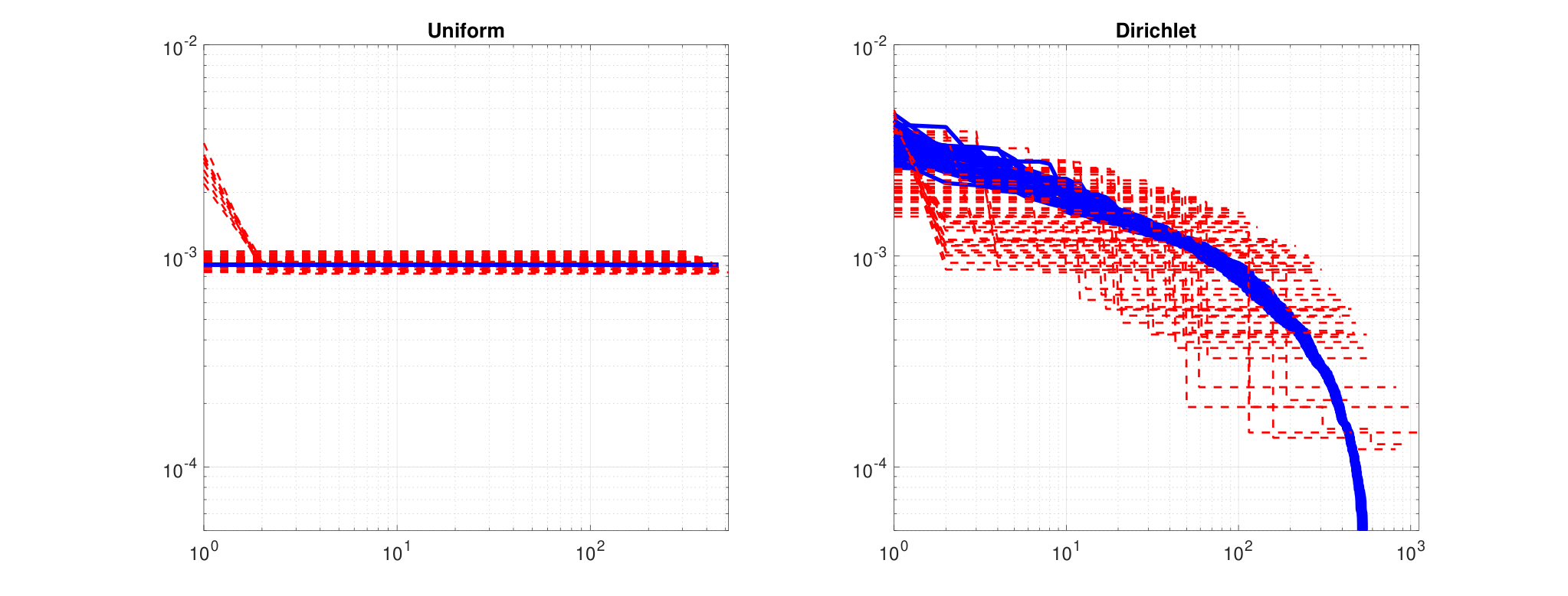
Refer to caption
Fig. 2: Actual and estimated distribution of missing letters (in descending order). Blue solid: actual, Red dashed: estimate.

We observe that the estimate is close to the actual distributions in all of the cases.

A similar plot for l=1l=1 is shown in Fig. 3.

Fig. 3: Actual and estimated distribution of letters that appear once (in descending order). Blue solid: actual, Red dashed: estimate.

As observed, the estimates vary more than the l=0l=0 case, and generally appear to be weaker than the results for l=0l=0. Therefore, it is important to theoretically study the limits of estimation of [px:x∈Sl(Xn)][p_{x}:x\in S_{l}(X^{n})] and associated quantities.

In summary, the generalization of missing mass that we have proposed offers the possibility of exploring the structure of the missing distribution and the sparsely observed distribution. We have demonstrated two explicit applications that test for uniformity of missing letters and attempt to estimate the distribution of missing letters and letters that occur once, up to ordering. These testing and estimation problems introduced above aim to infer more about the probabilities of the letters that were not seen in the samples, departing from the already well-studied measures like missing mass and the number of unseen letters (or species) that do a coarse characterization of the unseen part of P.P. Inferring the finer details about the missing probabilities, like the proximity of the missing part of the PP vector to uniformity or the individual probabilities of the missing letters, could lead to better estimation of PP from Xn.X^{n}.

II-C Concentration results and new tail bounds

II-C1 Prior Work

Various concentration results (uniform over all distributions PP) and tail bounds have been shown for missing mass M0​(Xn,P)M_{0}(X^{n},P) [7, 27, 21, 22, 28]. We quickly recall the general setting for such concentration results. For a random variable ZZ, let

LZ​(λ)≜log⁡(E⁡[eλ⁡(Z−E⁡[Z])])L_{Z}(\lambda)\triangleq\log(E[e^{\lambda(Z-E[Z])}]) (27)

denote the log Moment Generating Function (MGF). A random variable ZZ is said to be sub-Gaussian with variance factor vv, denoted Z∼sub-Gaussian​(v)Z\sim\text{sub-Gaussian}(v), on the right tail if LZ​(λ)≤λ2​v/2L_{Z}(\lambda)\leq\lambda^{2}v/2, λ>0\lambda>0. If ZZ is sub-Gaussian​(v)\text{sub-Gaussian}(v) on the right tail, by the standard Chernoff method, we have the right tail bound

Pr(Z≥E[Z]+ϵ)≤e−ϵ2/2v,ϵ≥0.\text{Pr}(Z\geq E[Z]+\epsilon)\leq e^{-\epsilon^{2}/2v},\ \epsilon\geq 0. (28)

For sub-Gaussian left tail bounds, we will need −Z∼sub-Gaussian​(v){-}Z\sim\text{sub-Gaussian}(v) on the right tail, or equivalently LZ​(λ)≤λ2​v/2L_{Z}(\lambda)\leq\lambda^{2}v/2, λ<0\lambda<0.

One of the first concentration results for missing mass was shown in [7], where a high probability bound on a letter not being seen in XnX^{n} is used in McDiarmid’s inequality [29] to show the right tail bound Pr(M0≥E[M0]+ϵ)≤e−nϵ2/3\text{Pr}(M_{0}\geq E[M_{0}]+\epsilon)\leq e^{-n\epsilon^{2}/3}, ϵ≥0\epsilon\geq 0. In [27], the above bound was improved to

Pr​(M0≥E⁡[M0]+ϵ)≤e−n​ϵ2,ϵ≥0,\text{Pr}(M_{0}\geq E[M_{0}]+\epsilon)\leq e^{-n\epsilon^{2}},\ \epsilon\geq 0, (29)

by showing that M0​(Xn,P)∼sub-Gaussian​(0.5/n),M_{0}(X^{n},P)\sim\text{sub-Gaussian}(0.5/n), for any PP, on the right tail using negative association and the Kearns-Saul inequality. Further, [27] showed the left tail bound Pr​(M0≤E⁡[M0]−ϵ)≤e−1.359​n​ϵ2\text{Pr}(M_{0}\leq E[M_{0}]-\epsilon)\leq e^{-1.359n\epsilon^{2}}, ϵ≥0\epsilon\geq 0, using negative association and connections between Chernoff entropy and Gibbs variance. In [21], the left tail bound was further improved to

Pr​(M0≤E⁡[M0]−ϵ)≤e−1.92​n​ϵ2,ϵ≥0,\text{Pr}(M_{0}\leq E[M_{0}]-\epsilon)\leq e^{-1.92n\epsilon^{2}},\ \epsilon\geq 0, (30)

by showing that −M0​(Xn,P)∼sub-Gaussian​(γ/n),-M_{0}(X^{n},P)\sim\text{sub-Gaussian}(\gamma/n), for any PP, on the right tail, where γ\gamma is defined as

γ=maxt>0⁡t​e−t​(1−e−t)=0.2603​…,(1/2​γ)=1.92​….\displaystyle\gamma=\max_{t>0}\,t\,e^{-t}(1-e^{-t})=0.2603\ldots,\ (1/2\gamma)=1.92\ldots. (31)

Remarks: As we show in Section VI-A, Var​(M0)≤γ/n\text{Var}(M_{0})\leq\gamma/n, and there exist uniform distributions that nearly achieve this variance upper bound [23]. Now, if Z∼sub-Gaussian​(v)Z\sim\text{sub-Gaussian}(v), it is known that v≥var​(Z)v\geq\text{var}(Z) [29]. So, the constant 1.92 in the left tail bound e−1.92​n​ϵ2e^{-1.92n\epsilon^{2}} is nearly optimal.

In our recent work [28], we provided evidence that the constant 1 is likely to be tight for the right tail bound e−n​ϵ2e^{-n\epsilon^{2}} in the sub-Gaussian regime. More precisely, we showed that, in the Poisson sampling model (N∼Poisson​(n)N\sim\text{Poisson}(n) samples), there exists PP such that M0​(XN,P)M_{0}(X^{N},P) is not sub-Gaussian​(c/n)\text{sub-Gaussian}(c/n) for c<0.5c<0.5.

Therefore, the best distribution free (i.e. uniform over all PP) asymptotic left and right tail bounds for M0M_{0} using sub-Gaussianity appear to be e−1.92​n​ϵ2e^{-1.92n\epsilon^{2}} and e−n​ϵ2e^{-n\epsilon^{2}}, respectively. However, it is interesting to consider tail bounds using other approaches such as sub-Poisson and sub-Gamma property [22], as these are known to improve upon sub-Gaussian tail bounds in some cases [29].

Extending concentration results from missing mass M0​(Xn,P)M_{0}(X^{n},P) to missing mass of functions M0,g​(Xn,P)M_{0,g}(X^{n},P) is challenging because the methods used for proving concentration results for M0M_{0} are specific to the missing mass M0M_{0} and to sub-Gaussian concentration results. For applications, obtaining the best possible concentration results by going beyond sub-Gaussianity, if necessary, is interesting and important.

II-C2 Our Results

To obtain concentration results and tail bounds for M0,g​(Xn,P)M_{0,g}(X^{n},P) that are distribution-free, a standard approach is to upper bound the log Moment Generating Function (log MGF) LM0,g​(λ)=log⁡E⁡[eλ⁡(M0,g−E⁡[M0,g])]L_{M_{0,g}}(\lambda)=\log E[e^{\lambda(M_{0,g}-E[M_{0,g}])}], by a function of λ\lambda, and use the Chernoff method. Now, M0,g=∑xg⁡(px)​I​(Nx=0)M_{0,g}=\sum_{x}g(p_{x})I(N_{x}=0), is a sum of random variables g⁡(px)​I​(Nx=0)g(p_{x})I(N_{x}=0), x∈𝒳x\in\mathcal{X}, which are (1) dependent because NxN_{x} are dependent, and (2) highly heterogeneous because of the range of values of pxp_{x}. To address dependency, we will follow [27] and use the idea of negative association. The log MGF of M0,gM_{0,g}

LM0,g​(λ)\displaystyle L_{M_{0,g}}(\lambda) =log⁡E⁡[∏x∈𝒳exp⁡{λ​g​(px)​[I⁡(Nx=0)−Pr​(Nx=0)]}]\displaystyle=\log E\left[\prod_{x\in\mathcal{X}}\exp\{\lambda g(p_{x})[I(N_{x}=0)-\text{Pr}(N_{x}=0)]\}\right]
≤(a)​∑x∈𝒳log⁡E⁡[exp⁡{λ​g​(px)​[I⁡(Nx=0)−Pr​(Nx=0)]}],\displaystyle\overset{(a)}{\leq}\sum_{x\in\mathcal{X}}\log E\left[\exp\{\lambda g(p_{x})[I(N_{x}=0)-\text{Pr}(N_{x}=0)]\}\right], (32)

where (a)(a) follows because of the following argument. The random variables NxN_{x}, x∈𝒳x\in\mathcal{X}, are negatively associated [7, 30] and

T⁡(Nx)≜exp⁡{λ​g​(px)​[I⁡(Nx=0)−Pr​(Nx=0)]}T(N_{x})\triangleq\exp\{\lambda g(p_{x})[I(N_{x}=0)-\text{Pr}(N_{x}=0)]\}

is a monotonically non-increasing function of NxN_{x}. So, T⁡(Nx)T(N_{x}), x∈𝒳x\in\mathcal{X}, are negatively associated [30] resulting in E⁡[T⁡(Nx)​T​(Nx′)]≤E⁡[T⁡(Nx)]​E​[T⁡(Nx′)]E[T(N_{x})T(N_{x^{\prime}})]\leq E[T(N_{x})]E[T(N_{x^{\prime}})].

Following the above simplification, to address the heterogeneity and decouple λ\lambda and pxp_{x}, [7, 21] use the Kearns-Saul inequality to upper bound E⁡[T⁡(Nx)]E[T(N_{x})]. An alternative method, introduced in [22], starts with Bennett’s inequality [29]. We will employ a stronger version of Bennett’s inequality for a zero-mean random variable ZZ with |Z|<1|Z|<1, which is proved as follows:

E⁡[exp⁡(t​Z)]\displaystyle E[\exp(tZ)] =(E⁡[Z]=0)​1+∑k=2∞tk​E​[Z2​Zk−2]k!\displaystyle\overset{(E[Z]=0)}{=}1+\sum_{k=2}^{\infty}\frac{t^{k}E[Z^{2}Z^{k-2}]}{k!}
≤(|Z|<1)​1+∑k=2∞tk​E​[Z2]k!\displaystyle\overset{(|Z|<1)}{\leq}1+\sum_{k=2}^{\infty}\frac{t^{k}E[Z^{2}]}{k!}
≤1+Var​(Z)​(et−t−1).\displaystyle\leq 1+\text{Var}(Z)(e^{t}-t-1). (33)

By using 1+x≤ex1+x\leq e^{x} on the RHS of (33) with x=Var​(Z)​(et−t−1)x=\text{Var}(Z)(e^{t}-t-1) and taking logarithms, we obtain the usual Bennett’s inequality, given below:

log⁡E⁡[exp⁡(t​Z)]≤Var​(Z)​(et−t−1), all ​t.\log E[\exp(t Z)]\leq\text{Var}(Z)(e^{t}-t-1),\text{ all }t. (34)

Setting t=λ​g​(px)t=\lambda g(p_{x}) and Z=I⁡(Nx=0)−Pr​(Nx=0)Z=I(N_{x}=0)-\text{Pr}(N_{x}=0) with Var​(Z)=(1−px)n​(1−(1−px)n)\text{Var}(Z)=(1-p_{x})^{n}(1-(1-p_{x})^{n}) in (33) and (34), and substituting the upper bounds in (32), we get the following two bounds on the log MGF:

LM0,g​(λ)\displaystyle L_{M_{0,g}}(\lambda) ≤∑x∈𝒳log⁡(1+(1−px)n​(1−(1−px)n)​(eλ​g​(px)−λ​g​(px)−1)),\displaystyle\leq\sum_{x\in\mathcal{X}}\log(1+(1-p_x)^n(1-(1-p_x)^n)(e^{\lambda g(p_x)}-\lambda g(p_x) - 1)), (35)
LM0,g​(λ)\displaystyle L_{M_{0,g}}(\lambda) ≤∑x∈𝒳(1−px)n​(1−(1−px)n)​(eλ​g​(px)−λ​g​(px)−1).\displaystyle\leq\sum_{x\in\mathcal{X}}(1-p_{x})^{n}(1-(1-p_{x})^{n})(e^{\lambda g(p_{x})}-\lambda g(p_{x})-1). (36)

To obtain distribution-free concentration results and tail bounds, the next step is to upper bound the RHS above by a function of λ\lambda (free of the distribution pxp_{x}) for λ>0\lambda>0 to obtain right tail bounds and λ<0\lambda<0 to obtain left tail bounds.

TABLE I: Types of concentration and tail bounds.
Type Upper bounding Function Range Tail bound Remarks
General f⁡(λ)f(\lambda) λ∈[s,t]\lambda\in[s,t] exp⁡{minλ∈[s,t]⁡f⁡(λ)−λ​ϵ}\exp\left\{\min\limits_{\lambda\in[s,t]}f(\lambda)-\lambda\epsilon\right\} Chernoff
Sub-Gaussian(σ2)(\sigma^{2}) σ2\sigma^{2}: variance parameter λ2​σ2/2\lambda^{2}\sigma^{2}/2 Right: λ>0\lambda>0 Left: λ<0\lambda<0 e−ϵ2/2σ2e^{-\epsilon^{2}/2\sigma^{2}} [29]
Sub-Gamma(v,c)(v,c) vv: variance parameter cc: scale parameter λ2​v/21−c​λ\dfrac{\lambda^{2}v/2}{1-c\lambda} Right: λ∈[0,1/c)\lambda\in[0,1/c) (38) [29]
Strongly-sub-Gamma(v,c)(v,c) vc2​log⁡e−λ​c1−c​λ\frac{v}{c^{2}}\log\dfrac{e^{-\lambda c}}{1-c\lambda} Right: λ∈[0,1/c)\lambda\in[0,1/c) (39) Proposed
Filtered sub-Gaussian(σ2,h⁡(λ))(\sigma^{2},h(\lambda)) h⁡(λ)h(\lambda): filter λ2​σ2/2+h⁡(λ)\lambda^{2}\sigma^{2}/2+h(\lambda) λ∈[s,t]\lambda\in[s,t] exp⁡{minλ∈[s,t]⁡λ2​σ2/2+h⁡(λ)−λ​ϵ}\exp\left\{\min\limits_{\lambda\in[s,t]}\lambda^{2}\sigma^{2}/2+h(\lambda)-\lambda\epsilon\right\} Proposed
Poly-sub-Gamma-filtered(R,𝐚,v,c)(R,\mathbf{a},v,c) RR: degree parameter 𝐚=[a2a3⋯aR]\mathbf{a}=[a_{2}\ a_{3}\ \cdots\ a_{R}] ∑r=2Rar​λrr+\sum\limits_{r=2}^{R}a_{r}\dfrac{\lambda^{r}}{r}+ vc2​log⁡e−λ​c1−c​λ\frac{v}{c^{2}}\log\dfrac{e^{-\lambda c}}{1-c\lambda} Right: λ∈[0,1/c)\lambda\in[0,1/c) R=2R=2: (40) R>2R>2: numerical Proposed

Table I shows the different forms of the upper-bounding function of λ\lambda along with the range of λ\lambda and associated tail bounds obtained by the Chernoff method. The first row describes the general Chernoff bounding method.

Sub-Gaussianity is a standard notion, and has been extensively studied for the case of missing mass where g⁡(p)=pg(p)=p. While sub-Gamma concentration is described in [29], we propose the notion of strongly sub-Gamma concentration, where the log-MGF is upper-bounded by (v/c2)​log⁡e−λ​c1−c​λ(v/c^{2})\log\frac{e^{-\lambda c}}{1-c\lambda}, which is the log-MGF of a Gamma random variable with variance parameter vv and scale parameter cc. Since the function λ2​v/21−c​λ\frac{\lambda^{2}v/2}{1-c\lambda}, introduced for sub-Gamma concentration in [29], does not correspond to the log-MGF of a Gamma random variable, the notion of strongly sub-Gamma concentration is, perhaps, a useful addition. It is easy to show the following implications:

Z∼sub-Gaussian​(v),λ>0→Z∼Strongly sub-Gamma​(v,c),c>0→Z∼sub-Gamma​(v,c).Z\sim\text{sub-Gaussian}(v),\,\lambda>0\to Z\sim\text{Strongly sub-Gamma}(v,c),\,c>0\to Z\sim\text{sub-Gamma}(v,c). (37)

Note that the variance factor vv with which a random variable ZZ can be sub-Gaussian or Strongly sub-Gamma or sub-Gamma is lower bounded by Var​(Z).\text{Var}(Z). So, while sub-Gaussianity is the strongest notion i.e. it gives the best tail bound for a given variance factor, the optimality of the variance factor is critical for obtaining the best possible tail bounds. If the variance factor of sub-Gaussian concentration does not coincide with the variance of ZZ, there is a possibility of the seemingly weaker notions of concentration, such as strongly sub-Gamma or sub-Gamma concentration with smaller variance factors than sub-Gaussian, resulting in better tail bounds on Pr​(Z>E​[Z]+ϵ)\text{Pr}(Z>E[Z]+\epsilon) for a restricted range of ϵ\epsilon, as illustrated for missing mass later on.

Next, we propose the notion of filtered sub-Gaussian concentration, where the log-MGF is upper-bounded by f⁡(λ)=λ2​σ2/2+h⁡(λ)f(\lambda)=\lambda^{2}\sigma^{2}/2+h(\lambda). In terms of distributions, this is equivalent to convolving a Gaussian distribution with another distribution with log-MGF h⁡(λ)h(\lambda) (assuming it is a valid log-MGF corresponding to some distribution). Hence, we use the terminology of “filtering” and call h⁡(λ)h(\lambda) as a filter. The convolution seemingly weakens concentration when compared to sub-Gaussian concentration. However, when the variance factor of sub-Gaussian concentration is not optimal, instead of bounding the tail with that of a Gaussian random variable of higher variance, one can possibly obtain better bounds by considering convolutions of a Gaussian random variable (with lower variance) and other random variables.

The last row of the table describes the specific type of filtering that is useful for missing mass, namely, filtering a Gamma log-MGF by a polynomial. When the degree parameter R=1R=1, this type of concentration reduces to strongly sub-Gamma concentration. When R=2R=2, the log-MGF upper bound λ2​a2/2+(v/c2)​log⁡e−λ​c1−c​λ\lambda^{2}a_{2}/2+(v/c^{2})\log\frac{e^{-\lambda c}}{1-c\lambda} corresponds to a random variable whose distribution is the convolution of a Gaussian random variable with variance a2a_{2} and a Gamma random variable with variance parameter vv and scale parameter cc. As we illustrate later, such convolutions improve the right tail bound for missing mass. For R>2R>2, the polynomial part may result in the filter not being a valid log-MGF, but the tail bounds are still valid, and can be computed numerically.

If Z∼sub-Gamma​(v,c)Z\sim\text{sub-Gamma}(v,c) on the right tail, we get the following tail bound using the standard Chernoff method:

Pr​(Z≥E⁡[Z]+ϵ)≤exp⁡{−(1+c​ϵv−1+2​c​ϵv)​vc2}.\text{Pr}(Z\geq E[Z]+\epsilon)\leq\exp\left\{-\left(1+\frac{c\epsilon}{v}-\sqrt{1+\frac{2c\epsilon}{v}}\right)\frac{v}{c^{2}}\right\}. (38)

Similarly, if Z∼Strongly sub-Gamma​(v,c)Z\sim\text{Strongly sub-Gamma}(v,c), we get

Pr​(Z≥E⁡[Z]+ϵ)≤exp⁡{−1c​(ϵ−vc​log⁡(1+c​ϵv))}.\text{Pr}(Z\geq E[Z]+\epsilon)\leq\exp\left\{-\frac{1}{c}\left(\epsilon-\frac{v}{c}\log\left(1+\frac{c\epsilon}{v}\right)\right)\right\}. (39)

Using the Taylor series bound ln⁡(1+x)≤x−0.5​x2+(1/3)​x3,x≥0,\ln(1+x)\leq x-0.5x^{2}+(1/3)x^{3},x\geq 0, on the RHS in (39), we get

Pr​(Z≥E⁡[Z]+ϵ)≤exp⁡{−ϵ22​v​(1−(2/3)​c​ϵv)}\text{Pr}(Z\geq E[Z]+\epsilon)\leq\exp\left\{-\frac{\epsilon^{2}}{2v}\left(1-({2}/{3})\frac{c\epsilon}{v}\right)\right\} (11)

Note that the exponent in the RHS of (11) is away by (1/3)​(c​ϵ3/v2)(1/3)(c\epsilon^{3}/v^{2}) from the exponent in the tail bound for sub-Gaussian​(v).\text{sub-Gaussian}(v). If Z∼Poly-sub-Gamma filtered​(R,𝐚,v,c)Z\sim\text{Poly-sub-Gamma filtered}(R,\mathbf{a},v,c), the minimization inside the exponent in Chernoff bound computation is easy to evaluate numerically for any RR because f′​(λ)f^{\prime}(\lambda) is rational in λ\lambda with a linear denominator. For R=2R=2, the tail bound can be expressed analytically as follows.

Pr​(Z−E⁡[Z]≥ϵ)≤exp⁡{−1c​((12−d2d1)​ϵ+vc​ln⁡(1−2​c​ϵd1))},\displaystyle\text{Pr}(Z-{E}[Z]\geq\epsilon)\leq\exp\left\{-\frac{1}{c}\left(\left(\frac{1}{2}-\frac{d_{2}}{d_{1}}\right)\epsilon+\frac{v}{c}\ln\left(1-\frac{2c\epsilon}{d_{1}}\right)\right)\right\}, (40)

where d1=(a2+v+c​ϵ)+(a2+v+c​ϵ)2−4​a2​c​ϵd_{1}=(a_{2}+v+c\epsilon)+\sqrt{(a_{2}+v+c\epsilon)^{2}-4a_{2}c\epsilon} and d2=a2−(v+c​ϵ)d_{2}=a_{2}-(v+c\epsilon). For a2≤v,a_{2}\leq v, we upper bound the exponent in the RHS of (40) with its corresponding third order Taylor series polynomial about ϵ=0,\epsilon=0, to get

Pr​(Z≥E⁡[Z]+ϵ)≤exp⁡{−ϵ22​(v+a2)​(1−(2/3)​c​v​ϵ(a2+v)2)}\text{Pr}(Z\geq E[Z]+\epsilon)\leq\exp\left\{-\frac{\epsilon^{2}}{2(v+a_{2})}\left(1-({2}/{3})\frac{cv\epsilon}{(a_{2}+v)^{2}}\right)\right\} (13)

Using the definitions and notation in Table I, we now describe our main concentration result for the missing mass of the function g⁡(p)g(p), M0,g​(Xn,P)M_{0,g}(X^{n},P), in Theorem 2. Let

ur∗​(n,g)\displaystyle u^{*}_{r}(n,g) ≜max0<p<1⁡g​(p)r​(1−p)n​1−(1−p)np.\displaystyle\triangleq\max_{0<p<1}g(p)^{r}(1-p)^{n}\,\dfrac{1-(1-p)^{n}}{p}. (41)

Where necessary, we will drop the arguments n,gn,g in ur∗​(n,g)u^{*}_{r}(n,g) to reduce clutter.

Theorem 2.
  1. 1.
    M0,g​(Xn,P)∼sub-Gaussian​(0.519​maxp​(g⁡(p)/p)2n),all ​λ∈ℝ.M_{0,g}(X^{n},P)\sim\text{sub-Gaussian}\left(\frac{0.519\max_{p}(g(p)/p)^{2}}{n}\right),\ \text{all }\lambda\in\mathbb{R}. (42)

    Additionally, on the left tail,

    M0,g​(Xn,P)∼sub-Gaussian​(u2∗​(n,g)),λ<0.M_{0,g}(X^{n},P)\sim\text{sub-Gaussian}(u^{*}_{2}(n,g)),\ \lambda<0. (43)
  2. 2.

    Let R≥1R\geq 1 be a positive integer. Let c>0c>0 be such that

    ur∗​(n,g)(r−1)!≤c​ur−1∗​(n,g)(r−2)!,r≥3.\frac{u^{*}_{r}(n,g)}{(r-1)!}\leq c\frac{u^{*}_{r-1}(n,g)}{(r-2)!},\ r\geq 3. (44)

    Let v=uR+1∗​(n,g)/(cR−1​R!)v=u^{*}_{R+1}(n,g)/(c^{R-1}R!), and

    ar=(ur∗​(n,g)(r−1)!−cr−2​v), 2≤r≤R.a_{r}=\left(\frac{u^{*}_{r}(n,g)}{(r-1)!}-c^{r-2}v\right),\ 2\leq r\leq R.

    Then, for 𝐚=[a2a3⋯aR]\mathbf{a}=[a_{2}\ a_{3}\ \cdots\ a_{R}], on the right tail,

    M0,g​(Xn,P)∼Poly-sub-Gamma-filtered​(R,𝐚,v,c).M_{0,g}(X^{n},P)\sim\text{Poly-sub-Gamma-filtered}(R,\mathbf{a},v,c). (45)

The first part of Theorem 2, proven in Section IV-A, provides a sub-Gaussian right-tail and left-tail bound as shown in Table I. For the case of missing mass, i.e. g⁡(p)=pg(p)=p, we have sub-Gaussianity with a variance of 0.519/n0.519/n, which is close to the best-known 0.5/n0.5/n. Additionally, since u2∗​(n,p)≤γ/nu^{*}_{2}(n,p)\leq\gamma/n (proved in Section VI-A; recall that γ=maxt>0⁡t​e−t​(1−e−t)=0.2603​…\gamma=\max_{t>0}\,t\,e^{-t}(1-e^{-t})=0.2603\ldots), this recovers the best-known distribution free or uniform sub-Gaussian left-tail bound e−1.92​n​ϵ2e^{-1.92n\epsilon^{2}}. Our proof of these tail bounds for M0M_{0} are arguably simpler compared to the Gibbs-variance method used in [27] or the Kearns-Saul inequality method used in [21]. For all other g⁡(p)g(p), such as g⁡(p)=pαg(p)=p^{\alpha} for power sum or g⁡(p)=p​log⁡(1/p)g(p)=p\log(1/p) for Shannon entropy, the sub-Gaussian concentration left tail results have been shown for the first time.

For the case of g⁡(p)=pαg(p)=p^{\alpha} and g⁡(p)=p​log2⁡(1/p)g(p)=p\log_{2}(1/p), we simplify the left tail bounds and present them in the following corollary.

Corollary 3.
  1. 1.

    The order-α\alpha missing mass M0,αM_{0,\alpha} for α≥1,\alpha\geq 1, satisfies

    Pr​(M0,α−E⁡[M0,α]≤−ϵ)≤exp⁡{−n2​α−1​ϵ22​γα},n≥(2​α−1)​ln⁡2/(2​α−1−ln⁡2),\displaystyle\text{Pr}(M_{0,\alpha}-{E}[M_{0,\alpha}]\leq-\epsilon)\leq\exp\left\{-\frac{n^{2\alpha-1}\epsilon^{2}}{2\gamma_{\alpha}}\right\},\quad n\geq(2\alpha-1)\ln 2/(2\alpha-1-\ln 2), (46)

    where γα=maxt>0⁡t2​α−1​e−t​(1−e−t)\gamma_{\alpha}=\max_{t>0}t^{2\alpha-1}e^{-t}(1-e^{-t}).

  2. 2.

    Let H0​(Xn,P)≜∑x∈𝒳px​log2⁡(1/px)​I​(Nx​(Xn)=0)H_{0}(X^{n},P)\triangleq\sum_{x\in\mathcal{X}}p_{x}\log_{2}(1/p_{x})I(N_{x}(X^{n})=0) be the missing Shannon entropy in XnX^{n} of a distribution P.P. H0​(Xn,P)H_{0}(X^{n},P) satisfies

    Pr​(H0−E⁡[H0]≤−ϵ)≤exp⁡{−n​ϵ22​γ​(log2​n)2},n≥3,\displaystyle\text{Pr}(H_{0}-{E}[H_{0}]\leq-\epsilon)\leq\exp\left\{-\frac{n\epsilon^{2}}{2\gamma(\log_{2}n)^{2}}\right\},\quad n\geq 3, (47)

    where γ=maxt>0⁡t​e−t​(1−e−t)=0.2603​…\gamma=\max_{t>0}te^{-t}(1-e^{-t})=0.2603\ldots.

The variance factors in the above uniform sub-Gaussian left tail bounds for M0,αM_{0,\alpha} and H0H_{0} are near optimal. A proof of Corollary 3 is given in Section VI.

The second part of Theorem 2, proven in Section IV-B, provides right tail bounds using the Poly-sub-Gamma-filtered approach with a Gamma MGF and a polynomial filter as described in Table I. The choice of the scale parameter cc needs elaboration. From (44), it is clear that cc quantifies the rate of decay of ur∗​(n,g)/(r−1)!u^{*}_{r}(n,g)/(r-1)!, and it will depend on the function g⁡(p)g(p). An important requirement is that cc should decay with nn so that the confidence intervals from the tail bounds shrink with increasing nn. The following rate of decay lemma describes the choice of cc as a decreasing function of nn for two types of functions g⁡(p)g(p).

Lemma 4.

Let g⁡(p)g(p) be differentiable for p∈(0,1)p\in(0,1), and let g′​(p)g^{\prime}(p) denote its derivative. Let ur∗​(n,g)u^{*}_{r}(n,g) be as defined in (41). There exist bib_{i}, 0≤i≤50\leq i\leq 5, independent of rr, such that

c=max⁡(b0​g​(b1/(n+b2)),b3​g​(b4/(n+b5)))​ satisfies ​ur∗​(n,g)(r−1)!≤c​ur−1∗​(n,g)(r−2)!,r≥3,c=\max(b_{0}\ g(b_{1}/(n+b_{2})),b_{3}\ g(b_{4}/(n+b_{5})))\text{ satisfies }\frac{u^{*}_{r}(n,g)}{(r-1)!}\leq c\frac{u^{*}_{r-1}(n,g)}{(r-2)!},\ r\geq 3, (48)

if g⁡(p)g(p) belongs to one of the following two types:

  1. 1.

    Type A: For some μ>0\mu>0,

    0<g′​(p)≤μ​g​(p)/p,p∈(0,1).0<g^{\prime}(p)\ \leq\ \mu\ g(p)/p,\ p\in(0,1).
  2. 2.

    Type B: For some p∗∈(0,1)p^{*}\in(0,1),

    0<g′​(p)\displaystyle 0<g^{\prime}(p) ≤(1/p−1/p∗)​g⁡(p)1−p,p∈(0,p∗),\displaystyle\leq(1/p-1/p^{*})\dfrac{g(p)}{1-p},\ p\in(0,p^{*}),
    g′​(p)\displaystyle g^{\prime}(p) <0,p∈(p∗,1).\displaystyle<0,\ \phantom{(1p-1/p^{*})\dfrac{g(p)}{1-p}}p\in(p^{*},1).

A proof of Lemma 4 is given in Section V. In the proof, the values of bib_{i} are explicitly specified for a g⁡(p)g(p) of Type A or B. Interesting examples such as g⁡(p)=pαg(p)=p^{\alpha}, α>0\alpha>0, belong to Type A with μ=α\mu=\alpha and g⁡(p)=p​log2⁡(1/p)g(p)=p\log_{2}(1/p) belongs to Type B with p∗=1/ep^{*}=1/e. For these cases, we further simplify the right tail bound for R=1R=1 (strongly sub-gamma concentration) in the following corollary.

Corollary 5.
  1. 1.

    The missing mass M0M_{0} satisfies

    Pr​(M0−E⁡[M0]≥ϵ)\displaystyle\text{Pr}(M_{0}-{E}[M_{0}]\geq\epsilon) ≤(a1)​exp⁡{−2​(n+2)3​(ϵ−2​γn3​log⁡(1+3​ϵ2​γn))},n≥3,\displaystyle\overset{(a_{1})}{\leq}\exp\left\{-\frac{2(n+2)}{3}\left(\epsilon-\frac{2\gamma_{n}}{3}\log\left(1+\frac{3\epsilon}{2\gamma_{n}}\right)\right)\right\},n\geq 3, (49)
    ≤(a2)​exp⁡{−1.92​n​ϵ2​(1−(ϵ/γn))},n≥3,\displaystyle{\color[rgb]{0,0,1}\overset{(a_{2})}{\leq}\exp\left\{-1.92n\epsilon^{2}(1-(\epsilon/\gamma_{n}))\right\},n\geq 3,} (50)
    Pr​(M0−E⁡[M0]≥ϵ)\displaystyle\text{Pr}(M_{0}-{E}[M_{0}]\geq\epsilon) ≤(a3)​exp⁡{−1.92​n​ϵ2​(1−(ψ/3​γ2)​ϵ)},n≥3,\displaystyle{\color[rgb]{0,0,1}\overset{(a_{3})}{\leq}\exp\left\{-1.92n\epsilon^{2}(1-(\psi/3\gamma^{2})\epsilon)\right\},n\geq 3,} (51)

    where γn=γ⁡(1+2/n)\gamma_{n}=\gamma(1+2/n), γ=maxt>0⁡t​e−t​(1−e−t)=0.2603​…,\gamma=\max_{t>0}te^{-t}(1-e^{-t})=0.2603\ldots, and ψ=maxt>0⁡t2​e−t​(1−e−t)=0.477​…\psi=\max_{t>0}t^{2}e^{-t}(1-e^{-t})=0.477\ldots.

  2. 2.

    Consider the order-α\alpha missing mass M0,αM_{0,\alpha}, α>1\alpha>1. For n>1+4​α2/(1−α)2n>1+4\alpha^{2}/(1-\alpha)^{2},

    Pr​(M0,α−E⁡[M0,α]≥ϵ)≤exp⁡{−n−ba​ϵ+γαa2​(n−b)3−2​α​log⁡(1+a​n2​α−1γα​(n−b)​ϵ)},\displaystyle\text{Pr}(M_{0,\alpha}-{E}[M_{0,\alpha}]\geq\epsilon)\leq\exp\left\{-\frac{n-b}{a}\epsilon+\frac{\gamma_{\alpha}}{a^{2}}(n-b)^{3-2\alpha}\log\left(1+\frac{an^{2\alpha-1}}{\gamma_{\alpha}(n-b)}\epsilon\right)\right\}, (52)

    where b=1+2​αα−1b=1+\frac{2\alpha}{\alpha-1}, a=(b−1)​(2​(α−1)α+1)αa=(b-1)\left(\frac{2(\alpha-1)}{\alpha+1}\right)^{\alpha} and γα=maxt>0⁡t2​α−1​e−t​(1−e−t)\gamma_{\alpha}=\max_{t>0}t^{2\alpha-1}e^{-t}(1-e^{-t}).

  3. 3.

    For the missing Shannon entropy in XnX^{n}, H0​(Xn,P)H_{0}(X^{n},P), of a distribution P,P,

    Pr​(H0−E⁡[H0]≥ϵ)\displaystyle\text{Pr}(H_{0}-{E}[H_{0}]\geq\epsilon) ≤(b1)​exp⁡{−2​n0log2​n0​(ϵ−γn′log2⁡(n0)​log⁡(1+ϵ​log2⁡(n0)γn′))},n≥3,\displaystyle\overset{(b_{1})}{\leq}\ \exp\{-\frac{2n_{0}}{\log_{2}n_{0}}\bigg(\epsilon-\frac{\gamma^{\prime}_{n}}{\log_{2}(n_{0})}\log\left(1+\epsilon\frac{\log_{2}(n_{0})}{\gamma^{\prime}_{n}}\right)\bigg)\bigg\},n\geq 3, (53)
    ≤(b2)​exp⁡{−n0​ϵ2γn′​(1−(2/3)​ϵ​log2​(n0)γn′)},n≥3,\displaystyle{\color[rgb]{0,0,1}\overset{(b_{2})}{\leq}\ \exp\{-\frac{n_{0}\epsilon^{2}}{\gamma^{\prime}_{n}}\bigg(1-(2/3)\frac{\epsilon\log_{2}(n_{0})}{\gamma^{\prime}_{n}}\bigg)\bigg\},n\geq 3,} (54)

    where n0=(1/3)​(n−1)+en_{0}=(1/3)(n-1)+e and γn′=2​γ​(1/3+(e−1/3)/n)​(log2​n)2\gamma^{\prime}_{n}=2\gamma(1/3+(e-1/3)/n)(\log_{2}n)^{2}.

Note that we get (49) by showing that M0M_{0} is strongly sub-gamma on the right tail with variance factor γ/n\gamma/n and scale parameter 3/2​(n+2)3/2(n+2) i.e. we have shown that M0M_{0} is uniformly strongly sub-gamma on the right tail with a near-optimal variance factor. We get the bound in (50) by using the right tail bound in (11) for a strongly sub-gamma(γ/n,3/2​(n+2))(\gamma/n,3/2(n+2)) random variable. We get the bound in (51) by showing that M0M_{0} is Poly-sub-Gamma-filtered with R=2,v=(1+2/n)​ψ/3​n,c=3/2​(n+2),R=2,v=(1+2/n)\ \psi/3n,c=3/2(n+2), and a=[a2]=[γ/n−v].a=[a_{2}]=[\gamma/n-v]. The bounds in (50), (51) are close to e−1.92​n​ϵ2e^{-1.92n\epsilon^{2}} (the best sub-gaussian left tail bound for M0M_{0}) for small ϵ.\epsilon. The variance factors in the uniform strongly sub-gamma results for the order-α\alpha missing mass and the missing Shannon entropy in (52), (53) respectively are also nearly-optimal. The bounds obtained for R=2,3​…,R=2,3\ldots, also have near-optimal variance factors that are non-increasing. A proof of Corollary 5 is given in Section VI.

For M0M_{0} (i.e. g⁡(p)=pg(p)=p), Fig. 4 shows a plot comparing the different right tail bounds for n=20,100,1000n=20,100,1000.

000.10.10.20.20.30.30.40.40.50.50.60.610−310^{-3}10−210^{-2}10−110^{-1}10010^{0}n=1000n{=}1000n=100n{=}100n=20n{=}20ϵ\epsilonPr​(M0−E⁡[M0]>ϵ)\text{Pr}(M_{0}-E[M_{0}]>\epsilon)Sub-GaussianR=2R=2R=5R=5
Fig. 4: Comparison of right tail bounds for M0M_{0}.

The new bounds, for R=2R=2 and R=5R=5, provide a noticeable improvement over the sub-Gaussian bound e−n​ϵ2e^{-n\epsilon^{2}} for all three values of nn over a significant range of ϵ\epsilon.

The proofs of the results in this section can be found in Section III and in the ensuing ones.

III Proof of Theorem 1

We start by proving the upper bound of Part 1 of the theorem.

III-A Upper bound on Rn,α∗R^{*}_{n,\alpha} for α∈ℕ\alpha\in\mathbb{N}

Consider the generalized Good-Turing estimator M0,αGT​(Xn)=ϕα​(Xn)(nα)M^{\textrm{GT}}_{0,\alpha}(X^{n})=\frac{\phi_{\alpha}(X^{n})}{\binom{n}{\alpha}}, α∈ℕ\alpha\in\mathbb{N}. By the definition of minimax risk, we have

Rn,α∗\displaystyle R_{n,\alpha}^{*} =minM^0,α⁡maxP⁡E⁡[(M^0,α​(Xn)−M0,α​(Xn,P))2]\displaystyle=\min_{\widehat{M}_{0,\alpha}}\max_{P}E[({\widehat{M}_{0,\alpha}}(X^{n})-M_{0,\alpha}(X^{n},P))^{2}]
≤maxP⁡E⁡[(M0,αGT​(Xn)−M0,α​(Xn,P))2]≜Rn,α​(M0,αGT).\displaystyle\leq\max_{P}E[(M^{\textrm{GT}}_{0,\alpha}(X^{n})-M_{0,\alpha}(X^{n},P))^{2}]\triangleq R_{n,\alpha}(M^{\textrm{GT}}_{0,\alpha}). (55)

The rest of the proof is to upper bound the worst-case squared-error risk of the generalized Good-Turing estimator Rn,α​(M0,αGT)R_{n,\alpha}(M^{\textrm{GT}}_{0,\alpha}), and this is provided in the next lemma.

Lemma 6.
Rn,α​(M0,αGT)≤O⁡(1/n2​α−1).\displaystyle R_{n,\alpha}(M^{\textrm{GT}}_{0,\alpha})\leq\ O\left(1/n^{2\alpha-1}\right). (56)
Proof.
(M0,αGT−M0,α)2\displaystyle(M^{\textrm{GT}}_{0,\alpha}-M_{0,\alpha})^{2} =(∑x∈𝒳1(nα)​I​(Nx=α)−pxα​I​(Nx=0))​(∑y∈𝒳1(nα)​I​(Ny=α)−pyα​I​(Ny=0))\displaystyle=\left(\sum_{x\in\mathcal{X}}\frac{1}{\binom{n}{\alpha}}I(N_{x}=\alpha)-p_{x}^{\alpha}I(N_{x}=0)\right)\left(\sum_{y\in\mathcal{X}}\frac{1}{\binom{n}{\alpha}}I(N_{y}=\alpha)-p_{y}^{\alpha}I(N_{y}=0)\right)
=[∑x∈𝒳(1(nα)2​I​(Nx=α)+px2​α​I​(Nx=0))]\displaystyle=\Bigg[\sum_{x\in\mathcal{X}}\bigg(\frac{1}{{\binom{n}{\alpha}}^{2}}I(N_{x}=\alpha)+p_{x}^{2\alpha}I(N_{x}=0)\bigg)\Bigg]
+[∑x∈𝒳∑y∈𝒳,y≠x1(nα)2​I​(Nx=Ny=α)−∑x∈𝒳∑y∈𝒳,y≠xpxα(nα)​I​(Nx=0,Ny=α)]\displaystyle\quad+\Bigg[\sum_{x\in\mathcal{X}}\sum_{y\in\mathcal{X},y\neq x}\frac{1}{{\binom{n}{\alpha}}^{2}}I(N_{x}=N_{y}=\alpha)-\sum_{x\in\mathcal{X}}\sum_{y\in\mathcal{X},y\neq x}\frac{p_{x}^{\alpha}}{\binom{n}{\alpha}}I(N_{x}=0,N_{y}=\alpha)\Bigg]
−[∑x∈𝒳∑y∈𝒳,y≠xpyα(nα)​I​(Ny=0,Nx=α)−∑x∈𝒳∑y∈𝒳,y≠x(px​py)α​I​(Nx=Ny=0)]\displaystyle\quad-\Bigg[\sum_{x\in\mathcal{X}}\sum_{y\in\mathcal{X},y\neq x}\frac{p_{y}^{\alpha}}{\binom{n}{\alpha}}I(N_{y}=0,N_{x}=\alpha)-\sum_{x\in\mathcal{X}}\sum_{y\in\mathcal{X},y\neq x}(p_{x}p_{y})^{\alpha}I(N_{x}=N_{y}=0)\Bigg] (57)

Taking expectations, we consider each of the terms inside square brackets above and bound them by O⁡(1/n2​α−1)O(1/n^{2\alpha-1}).

The following bounds are used repeatedly in the simplifications. Let f1:[0,1]→ℝ+f_{1}:[0,1]\to\mathbb{R}^{+} and f2:[0,1]2→ℝ+f_{2}:[0,1]^{2}\to\mathbb{R}^{+} be non-negative functions, and let aa, bb, cc be positive numbers.

∑xpx​f1​(px)\displaystyle\sum_{x}p_{x}f_{1}(p_{x}) ≤maxp∈[0,1]⁡f1​(p)\displaystyle\leq\max_{p\in[0,1]}f_{1}(p) (58)
∑x∑ypx​py​f2​(px,py)\displaystyle\sum_{x}\sum_{y}p_{x}p_{y}f_{2}(p_{x},p_{y}) ≤maxp,q∈[0,1]⁡f2​(p,q)\displaystyle\leq\max_{p,q\in[0,1]}f_{2}(p,q) (59)
maxp∈[0,1]⁡pa​(1−p)b\displaystyle\max_{p\in[0,1]}p^{a}(1-p)^{b} =aa​bb(a+b)a+b\displaystyle=\dfrac{a^{a}b^{b}}{(a+b)^{a+b}} (60)
maxp,q∈[0,1]p+q≤1⁡pa​qb​(1−p−q)c\displaystyle\max_{\begin{subarray}{c}p,q\in[0,1]\\ p+q\leq 1\end{subarray}}p^{a}q^{b}(1-p-q)^{c} =aa​bb​cc(a+b+c)a+b+c\displaystyle=\dfrac{a^{a}b^{b}c^{c}}{(a+b+c)^{a+b+c}} (61)

Let us first consider the first term in square brackets in (57).

∑x∈𝒳E⁡(1(nα)2​I​(Nx=α)+px2​α​I​(Nx=0))\displaystyle\sum_{x\in\mathcal{X}}E\left(\frac{1}{{\binom{n}{\alpha}}^{2}}I(N_{x}=\alpha)+p_{x}^{2\alpha}I(N_{x}=0)\right) =∑x∈𝒳1(nα)​pxα​(1−px)n−α+∑x∈𝒳px2​α​(1−px)n\displaystyle=\sum_{x\in\mathcal{X}}\frac{1}{{\binom{n}{\alpha}}}p_{x}^{\alpha}(1-p_{x})^{n-\alpha}+\sum_{x\in\mathcal{X}}p_{x}^{2\alpha}(1-p_{x})^{n}
≤(a)​1(nα)​(α−1)α−1​(n−α)n−α(n−1)n−1+(2​α−1)2​α−1​(n)n(n+2​α−1)n+2​α−1\displaystyle\overset{(a)}{\leq}\frac{1}{{\binom{n}{\alpha}}}\frac{(\alpha-1)^{\alpha-1}(n-\alpha)^{n-\alpha}}{(n-1)^{n-1}}+\frac{(2\alpha-1)^{2\alpha-1}(n)^{n}}{(n+2\alpha-1)^{n+2\alpha-1}}
≤O⁡(1n2​α−1),\displaystyle\leq O\left(\frac{1}{n^{2\alpha-1}}\right), (62)

where (a)(a) uses (58), (60). Next, we consider the second term in square brackets in (57). We will need the notation (na,b)=n!a!​b!​(n−a−b)!\binom{n}{a,b}=\frac{n!}{a!b!(n-a-b)!}. Further, we will assume n>2​αn>2\alpha.

∑x∈𝒳∑y∈𝒳,y≠xE⁡(1(nα)2​I​(Nx=Ny=α)−pxα(nα)​I​(Nx=0,Ny=α))\displaystyle\sum_{x\in\mathcal{X}}\sum_{y\in\mathcal{X},y\neq x}E\bigg(\frac{1}{{\binom{n}{\alpha}}^{2}}I(N_{x}=N_{y}=\alpha)-\frac{p_{x}^{\alpha}}{\binom{n}{\alpha}}I(N_{x}=0,N_{y}=\alpha)\bigg)
=∑x∈𝒳∑y∈𝒳,y≠x(px​py)α​((nα,α)(nα)2​(1−px−py)n−2​α−(1−px−py)n−α)\displaystyle\qquad\qquad\qquad\qquad=\sum_{x\in\mathcal{X}}\sum_{y\in\mathcal{X},y\neq x}(p_{x}p_{y})^{\alpha}\bigg(\frac{\binom{n}{\alpha,\alpha}}{{\binom{n}{\alpha}}^{2}}(1-p_{x}-p_{y})^{n-2\alpha}-(1-p_{x}-p_{y})^{n-\alpha}\bigg)
≤(a)​∑x∈𝒳∑y∈𝒳,y≠x(px​py)α​(1−px−py)n−2​α​(1−(1−px−py)α)\displaystyle\qquad\qquad\qquad\qquad\overset{(a)}{\leq}\sum_{x\in\mathcal{X}}\sum_{y\in\mathcal{X},y\neq x}(p_{x}p_{y})^{\alpha}(1-p_{x}-p_{y})^{n-2\alpha}(1-(1-p_{x}-p_{y})^{\alpha})
=(b)​∑x∈𝒳∑y∈𝒳,y≠x(px​py)α​(px+py)​(∑i=0α−1(1−px−py)n−2​α+i)\displaystyle\qquad\qquad\qquad\qquad\overset{(b)}{=}\sum_{x\in\mathcal{X}}\sum_{y\in\mathcal{X},y\neq x}(p_{x}p_{y})^{\alpha}(p_{x}+p_{y})\left(\sum_{i=0}^{\alpha-1}(1-p_{x}-p_{y})^{n-2\alpha+i}\right)
=(c)​2​∑i=0α−1∑x∈𝒳∑y∈𝒳,y≠xpx​py​(pxα​pyα−1​(1−px−py)n−2​α+i)\displaystyle\qquad\qquad\qquad\qquad\overset{(c)}{=}2\sum_{i=0}^{\alpha-1}\sum_{x\in\mathcal{X}}\sum_{y\in\mathcal{X},y\neq x}p_{x}p_{y}\Big(p_{x}^{\alpha}p_{y}^{\alpha-1}(1-p_{x}-p_{y})^{n-2\alpha+i}\Big)
≤(d)​2​∑i=0α−1αα​(α−1)α−1​(n−2​α+i)n−2​α+i(n+i−1)n+i−1\displaystyle\qquad\qquad\qquad\qquad\overset{(d)}{\leq}2\sum_{i=0}^{\alpha-1}\frac{\alpha^{\alpha}(\alpha-1)^{\alpha-1}(n-2\alpha+i)^{n-2\alpha+i}}{(n+i-1)^{n+i-1}}
≤O⁡(1n2​α−1),\displaystyle\qquad\qquad\qquad\qquad\leq O\left(\frac{1}{n^{2\alpha-1}}\right), (63)

where (a)(a) follows because (nα,α)≤(nα)2\binom{n}{\alpha,\alpha}\leq\binom{n}{\alpha}^{2}, (b)(b) follows using the identity 1−(1−a)m=a​∑i=0m−1(1−a)i1-(1-a)^{m}=a\sum_{i=0}^{m-1}(1-a)^{i}, (c)(c) follows because of the symmetry between xx and yy in the summation, and (d)(d) uses (59), (61).

Finally, we consider the third term in square brackets in (57).

∑x∈𝒳∑y∈𝒳,y≠xE⁡(pyα(nα)​I​(Nx=α,Ny=0)−(px​py)α​I​(Nx=Ny=0))\displaystyle\sum_{x\in\mathcal{X}}\sum_{y\in\mathcal{X},y\neq x}E\bigg(\frac{p_{y}^{\alpha}}{\binom{n}{\alpha}}I(N_{x}=\alpha,N_{y}=0)-(p_{x}p_{y})^{\alpha}I(N_{x}=N_{y}=0)\bigg)
=∑x∈𝒳∑y∈𝒳,y≠x(px​py)α​(1−px−py)n−α​(1−(1−px−py)α)\displaystyle\qquad\qquad\qquad\qquad=\sum_{x\in\mathcal{X}}\sum_{y\in\mathcal{X},y\neq x}(p_{x}p_{y})^{\alpha}(1-p_{x}-p_{y})^{n-\alpha}(1-(1-p_{x}-p_{y})^{\alpha})
≤O⁡(1n2​α−1),\displaystyle\qquad\qquad\qquad\qquad\leq O\left(\frac{1}{n^{2\alpha-1}}\right), (64)

where the final inequality follows using steps similar to those used to obtain (63). Using (62), (63) and (64), the proof is complete. ∎

III-B Lower bound on minimax risk Rn,α∗R^{*}_{n,\alpha}

The lower bound of O⁡(1/n2​α−1)O\left({1}/{n^{2\alpha-1}}\right) for all α∈ℕ\alpha\in\mathbb{N} is obtained by following the Dirichlet prior approach. This approach was used in [23] for the case of missing mass M0M_{0} with α=1\alpha=1. The same approach is generalized here for α∈ℕ\alpha\in\mathbb{N}.

Let Δk\Delta_{k} be the set of all probability distributions on the alphabet 𝒳={1,2,…,k}\mathcal{X}=\{1,2,\ldots,k\}. Let PP be a random variable on Δk\Delta_{k}, generated according to a Dirichlet distribution [31] with parameters 𝜷=(β1,β2,…,βk)\bm{\beta}=(\beta_{1},\beta_{2},\ldots,\beta_{k}). From the family of distributions Δk\Delta_{k}, PP is chosen according to Dirichlet(𝜷)(\bm{\beta}) and then Xn∼PX^{n}\sim P is sampled iid. By the standard prior method, the minimax rate Rn,α∗R^{*}_{n,\alpha} is lower bounded as

Rn,α∗\displaystyle R^{*}_{n,\alpha} ≥EXn​[Var​[M0,α​(Xn,P)|Xn]],\displaystyle\geq E_{X^{n}}\left[\text{Var}[M_{0,\alpha}(X^{n},P)|X^{n}]\right], (65)

where Var​[M0,α​(Xn,P)|Xn]\text{Var}\left[M_{0,\alpha}(X^{n},P)|X^{n}\right] is the conditional variance of M0,α​(Xn,P)M_{0,\alpha}(X^{n},P) conditioned on XnX^{n}.

Lemma 7.

Let P∼Dirichlet​(β1,β2,…,βk)P\sim\text{Dirichlet}(\beta_{1},\beta_{2},\ldots,\beta_{k}) with k=c​n2k=cn^{2}, c>0c>0, and βi=1/n\beta_{i}=1/n. Let Xn∼PX^{n}\sim P, iid. Then,

EXn[Var[M0,α(Xn,P)|Xn]]≥nO(1/n2​α−1),E_{X^{n}}\left[\text{Var}\left[M_{0,\alpha}(X^{n},\ P)|X^{n}\right]\ \right]\ \geq_{n}\ O\left(1/n^{2\alpha-1}\right), (66)

where the notation ≥n\geq_{n} is as defined in Section .

Proof.

A proof is given in Appendix -A. ∎

Combining Lemma 7 and (65), the proof of the lower bound is complete.

IV Proof of Theorem 2

IV-A Proof of Part 1 of Theorem 2

Starting with (35), we simplify as follows:

LM0,g​(λ)\displaystyle L_{M_{0,g}}(\lambda) ≤(a)​∑xlog⁡(1+e−n​px​(eλ​g​(px)−λ​g​(px)−1))\displaystyle\overset{(a)}{\leq}\sum_{x}\log(1+e^{-np_x}(e^{\lambda g(p_x)}-\lambda g(p_x) - 1))
=λ2n​∑xpx​[nλ2​px​log⁡(1+e−n​px​(eλ​g​(px)−λ​g​(px)−1))]\displaystyle=\frac{\lambda^{2}}{n}\sum_{x}p_{x}\left[\frac{n}{\lambda^{2}p_{x}}\log(1+e^{-np_x}(e^{\lambda g(p_x)}-\lambda g(p_x) - 1))\right]
≤(b)​λ2n​maxp​[nλ2​p​log⁡(1+e−n​p​(eλ​g​(p)−λ​g​(p)−1))]\displaystyle\overset{(b)}{\leq}\frac{\lambda^{2}}{n}\max_{p}\left[\frac{n}{\lambda^{2}p}\log(1+e^{-np}(e^{\lambda g(p)}-\lambda g(p) - 1))\right]
=λ2n​maxp​[(g⁡(p)p)2​n​p(λ​g​(p))2​log⁡(1+e−n​p​(eλ​g​(p)−λ​g​(p)−1))]\displaystyle=\frac{\lambda^{2}}{n}\max_{p}\left[\left(\frac{g(p)}{p}\right)^{2}\frac{np}{(\lambda g(p))^{2}}\log(1+e^{-np}(e^{\lambda g(p)}-\lambda g(p) - 1))\right]
≤λ2n​maxp​(g⁡(p)p)2​maxu,v​uv2​log⁡(1+e−u​(ev−v−1))\displaystyle\leq\frac{\lambda^{2}}{n}\max_{p}\left(\frac{g(p)}{p}\right)^{2}\ \max_{u,v}\frac{u}{v^{2}}\log(1+e^{-u}(e^v-v-1))
≤(c)​0.2595​λ2​maxp​(g⁡(p)/p)2n,\displaystyle\overset{(c)}{\leq}\frac{0.2595\lambda^{2}\max_{p}(g(p)/p)^{2}}{n}, (67)

where (a)(a) follows by using (1−px)n​(1−(1−px)n)≤(1−px)n≤e−n​px(1-p_{x})^{n}(1-(1-p_{x})^{n})\leq(1-p_{x})^{n}\leq e^{-np_{x}}, (b)(b) follows because average is lesser than maximum, and (c)(c) follows because maxu,v⁡uv2​log⁡(1+e−u​(ev−v−1))=0.2595​…\max_{u,v}\frac{u}{v^{2}}\log(1+e^{-u}(e^v-v-1))=0.2595... using some calculus and computations. From (67), we get the sub-Gaussianity result in (42).

Recall, from (36), the upper bound

LM0,g​(λ)≤∑x∈𝒳(1−px)n​(1−(1−px)n)​(eλ​g​(px)−λ​g​(px)−1).L_{M_{0,g}}(\lambda)\leq\sum_{x\in\mathcal{X}}(1-p_{x})^{n}(1-(1-p_{x})^{n})(e^{\lambda g(p_{x})}-\lambda g(p_{x})-1).

Since we are concerned with the left tail bound, we consider λ<0\lambda<0. Using et−t−1≤t2/2e^{t}-t-1\leq t^{2}/2, t≤0t\leq 0, and setting t=λ​g​(px)t=\lambda g(p_{x}), we get

LM0,g​(λ)\displaystyle L_{M_{0,g}}(\lambda) ≤∑x∈𝒳(1−px)n​(1−(1−px)n)​(λ​g​(px))22\displaystyle\leq\sum_{x\in\mathcal{X}}(1-p_{x})^{n}(1-(1-p_{x})^{n})\frac{(\lambda g(p_{x}))^{2}}{2}
≤λ2​u2∗​(n,g)2,λ≤0,\displaystyle\leq\frac{\lambda^{2}u^{*}_{2}(n,g)}{2},\quad\lambda\leq 0, (68)

where u2∗​(n,g)u^{*}_{2}(n,g) is as defined in (41). This completes the proof of Part 1 of Theorem 2.

IV-B Proof of Part 2 of Theorem 2

For right tail bounds, we consider λ>0\lambda>0. The following lemma provides a power series upper bound on LM0,g​(λ)L_{M_{0,g}}(\lambda) and is critical in the proof of Part 2 of Theorem 2.

Lemma 8 (Power series upper bound).
LM0,g​(λ)≤∑r=2∞λrr!​ur∗​(n,g),λ>0,L_{M_{0,g}}(\lambda)\leq\sum_{r=2}^{\infty}\frac{\lambda^{r}}{r!}u_{r}^{*}(n,g),\quad\lambda>0, (69)

where ur∗​(n,g)u^{*}_{r}(n,g) is as defined in (41).

Proof.

Using et−t−1=∑r=2∞trr!,t≥0,e^{t}-t-1=\sum_{r=2}^{\infty}\frac{t^{r}}{r!},t\geq 0, with t=λ​g​(px)t=\lambda g(p_{x}) in (36), we get

LM0,g​(λ)\displaystyle L_{M_{0,g}}(\lambda) ≤∑x∈𝒳(1−px)n​(1−(1−px)n)​(∑r=2∞(λ​g​(px))rr!)\displaystyle\leq\sum_{x\in\mathcal{X}}(1-p_{x})^{n}(1-(1-p_{x})^{n})\left(\sum_{r=2}^{\infty}\frac{(\lambda g(p_{x}))^{r}}{r!}\right)
=∑r=2∞λrr!​(∑x∈𝒳g​(px)r​(1−px)n​(1−(1−px)n))\displaystyle=\sum_{r=2}^{\infty}\frac{\lambda^{r}}{r!}\left(\sum_{x\in\mathcal{X}}g(p_{x})^{r}(1-p_{x})^{n}(1-(1-p_{x})^{n})\right)
=∑r=2∞λrr!​(∑x∈𝒳px​g​(px)r​(1−px)n​(1−(1−px)n)px)\displaystyle=\sum_{r=2}^{\infty}\frac{\lambda^{r}}{r!}\left(\sum_{x\in\mathcal{X}}p_{x}\ g(p_{x})^{r}(1-p_{x})^{n}\frac{(1-(1-p_{x})^{n})}{p_{x}}\right)
≤(a)​∑r=2∞λrr!​ur∗​(n,g),λ≥0,\displaystyle\overset{(a)}{\leq}\sum_{r=2}^{\infty}\frac{\lambda^{r}}{r!}u_{r}^{*}(n,g),\quad\lambda\geq 0,

where (a) follows by using (58) for λ≥0\lambda\geq 0. ∎

Let R≥1.R\geq 1. For r≥R+2r\geq R+2, repeatedly applying ur∗​(n,g)(r−1)!≤c​ur−1∗​(n,g)(r−2)!,r≥3\frac{u^{*}_{r}(n,g)}{(r-1)!}\leq c\,\frac{u^{*}_{r-1}(n,g)}{(r-2)!},\,r\geq 3, we have

ur∗​(n,g)(r−1)!≤cr−(R+1)​uR+1∗​(n,g)R!,r≥R+1.\frac{u^{*}_{r}(n,g)}{(r-1)!}\leq c^{r-(R+1)}\,\frac{u^{*}_{R+1}(n,g)}{R!},\,r\geq R+1. (70)

Omitting the arguments n,gn,g from ur∗​(n,g)u^{*}_{r}(n,g) for brevity and using the above inequality in (69), we get

LM0,g​(λ)\displaystyle L_{M_{0,g}}(\lambda) ≤∑r=2Rλrr!​ur∗+∑r=R+1∞λrr​cr−(R+1)​uR+1∗(R)!,\displaystyle\leq\sum_{r=2}^{R}\frac{\lambda^{r}}{r!}\,u^{*}_{r}+\sum_{r=R+1}^{\infty}\frac{\lambda^{r}}{r}\,c^{r-(R+1)}\,\frac{u^{*}_{R+1}}{(R)!},
=∑r=2Rλrr!​ur∗+uR+1∗cR+1​R!​∑r=R+1∞(c​λ)rr,\displaystyle=\sum_{r=2}^{R}\frac{\lambda^{r}}{r!}\,u^{*}_{r}+\frac{u^{*}_{R+1}}{c^{R+1}R!}\sum_{r=R+1}^{\infty}\frac{(c\lambda)^{r}}{r},
=(a)​(∑r=2Rλrr!​(ur∗−cr−2​v​(r−1)!))−vc2​(c​λ)+vc2​(∑r=1∞(c​λ)rr),\displaystyle\overset{(a)}{=}\left(\sum_{r=2}^{R}\frac{\lambda^{r}}{r!}\,(u^{*}_{r}-c^{r-2}v(r-1)!)\right)-\frac{v}{c^{2}}(c\lambda)+\frac{v}{c^{2}}\left(\sum_{r=1}^{\infty}\frac{(c\lambda)^{r}}{r}\right), (71)

where (a)(a) follows by setting v≜uR+1∗cR−1​R!v\triangleq\frac{u^{*}_{R+1}}{c^{R-1}R!} and adding/subtracting terms between the two summations. Using the Taylor expansion −log⁡(1−x)=∑r=1∞xrr-\log(1-x)=\sum_{r=1}^{\infty}\frac{x^{r}}{r}, x<1x<1, completes the proof.

V Proof of Lemma 4

In this section, we present a proof for Lemma 4. Let

ur​(p,n,g)≜g​(p)r​(1−p)n​(1−(1−p)n)/pu_{r}(p,n,g)\triangleq g(p)^{r}(1-p)^{n}(1-(1-p)^{n})/p

be the function that is maximized over p∈(0,1)p\in(0,1) in (41), and let pr∗=arg​maxp∈(0,1)⁡ur​(p,n,g)p^{*}_{r}=\argmax_{p\in(0,1)}u_{r}(p,n,g). So, we have ur∗​(n,g)=ur​(pr∗,n,g)u_{r}^{*}(n,g)=u_{r}(p^{*}_{r},n,g). In the next lemma, we upper bound the rate of fall of ur∗​(n,g)/(r−1)!u_{r}^{*}(n,g)/(r-1)! using pr∗p^{*}_{r}.

Lemma 9.
ur∗​(n,g)(r−1)!≤g⁡(pr∗)r−1​ur−1∗​(n,g)(r−2)!,r≥3.\frac{u_{r}^{*}(n,g)}{(r-1)!}\ \leq\ \frac{g(p^{*}_{r})}{r-1}\ \frac{u_{r-1}^{*}(n,g)}{(r-2)!},r\geq 3. (72)
Proof.

By the definition of ur​(p,n,g),ur∗​(n,g)u_{r}(p,n,g),u_{r}^{*}(n,g) and pr∗p^{*}_{r} we get

ur∗​(n,g)(r−1)!\displaystyle\frac{u^{*}_{r}(n,g)}{(r-1)!}\ =ur​(pr∗,n,g)(r−1)!​=(a)​g⁡(pr∗)r−1​ur−1​(pr∗,n,g)(r−2)!​≤(b)​g⁡(pr∗)r−1​ur−1∗​(n,g)(r−2)!,\displaystyle=\ \frac{u_{r}(p^{*}_{r},n,g)}{(r-1)!}\ \overset{(a)}{=}\ \frac{g(p^{*}_{r})}{r-1}\ \frac{u_{r-1}(p^{*}_{r},n,g)}{(r-2)!}\ \overset{(b)}{\leq}\ \frac{g(p^{*}_{r})}{r-1}\ \frac{u^{*}_{r-1}(n,g)}{(r-2)!},

where (a)(a) follows from ur​(p,n,g)=g⁡(p)​ur−1​(p,n,g)u_{r}(p,n,g)=g(p)u_{r-1}(p,n,g) and (b)(b) follows from ur−1​(pr∗,n,g)≤ur−1∗​(n,g)u_{r-1}(p^{*}_{r},n,g)\leq u^{*}_{r-1}(n,g). ∎

In the rest of the proof, we find an upper bound on c⁡(r)≜g⁡(pr∗)r−1c(r)\triangleq\frac{g(p^{*}_{r})}{r-1} that is independent of rr and decreasing with nn for functions g⁡(p)g(p) that are differentiable for p∈(0,1)p\in(0,1) and fall under either Type A or Type B as described in Lemma 4. Recall that g′​(p)g^{\prime}(p) denotes the derivative of g⁡(p)g(p).

Type A: For this type, we have that for some μ>0\mu>0,

0<g′​(p)≤μ​g​(p)/p,p∈(0,1).0<g^{\prime}(p)\leq\mu\ g(p)/p,\ p\in(0,1).

Taking partial derivative of ur​(p,n,g)u_{r}(p,n,g) with respect to pp, letting q≜1−pq\triangleq 1-p and simplifying, we get

∂ur​(p,n,g)∂p\displaystyle\partialderivative{ u_{r}(p,n,g)}{p} =qn−1p2​g​(p)r−1​(n​p​qn​g​(p)+(1−qn)​[((r−1)​q−n​p)​g​(p)+r​p​q​(g′​(p)−g⁡(p)p)]).\displaystyle=\frac{q^{n-1}}{p^{2}}\,g(p)^{r-1}\bigg(npq^{n}g(p)+(1-q^{n})\bigg[((r-1)q-np)g(p)+rpq\left(g^{\prime}(p)-\frac{g(p)}{p}\right)\bigg]\bigg). (73)

Using g′​(p)≤μ​g⁡(p)pg^{\prime}(p)\leq\mu\frac{g(p)}{p} in the above equation, we get

∂ur​(p,n,g)∂p\displaystyle\partialderivative{u_{r}(p,n,g)}{p} ≤qn−1p2​g​(p)r​(n​p​qn+(1−qn)​[r​μ−1−(n+r​μ−1)​p])\displaystyle\leq\frac{q^{n-1}}{p^{2}}\,g(p)^{r}\big(npq^{n}+(1-q^{n})\big[r\mu-1-(n+r\mu-1)p\big]\big)
<(a)​0, if ​r​μ−1−(n+r​μ−1)​p<−1,\displaystyle\overset{(a)}{<}0,\text{ if }r\mu-1-(n+r\mu-1)p<-1, (74)

where (a)(a) follows because n​p​qn−(1−qn)<0npq^{n}-(1-q^{n})<0. So, ur​(p,n,g)u_{r}(p,n,g) decreases for p>r​μ/(n+r​μ−1)p>r\mu/(n+r\mu-1) implying that

pr∗≤r​μn+r​μ−1.p^{*}_{r}\leq\frac{r\mu}{n+r\mu-1}.

Since g⁡(p)g(p) is an increasing function (g′​(p)>0g^{\prime}(p)>0),

c⁡(r)=g⁡(pr∗)r−1≤1r−1​g​(r​μn+r​μ−1),r≥3.c(r)=\frac{g(p^{*}_{r})}{r-1}\leq\frac{1}{r-1}\ g\left(\frac{r\mu}{n+r\mu-1}\right),r\geq 3. (75)

In the next lemma, we present upper bounds on 1r−1​g​(r​μn+r​μ−1)\frac{1}{r-1}\ g\left(\frac{r\mu}{n+r\mu-1}\right) that are independent of rr and are in the form of (48) for different ranges of μ\mu and nn.

Lemma 10.
  1. 1.

    If either 0<μ≤10<\mu\leq 1, or μ>1\mu>1 and n<1+4​μ2(μ−1)2n<1+\frac{4\mu^{2}}{(\mu-1)^{2}},

    c⁡(r)≤0.5​g​(3​μn+3​μ−1).c(r)\leq 0.5\ g\left(\frac{3\mu}{n+3\mu-1}\right).

    To get the form of (48), set b0=b3=0.5b_{0}=b_{3}=0.5, b1=b4=3​μb_{1}=b_{4}=3\mu and b2=b5=3​μ−1b_{2}=b_{5}=3\mu-1.

  2. 2.

    For μ>1\mu>1 and n≥1+4​μ2(μ−1)2n\geq 1+\frac{4\mu^{2}}{(\mu-1)^{2}},

    c⁡(r)≤max⁡(0.5​g​(3​μn+3​μ−1),1r2−1​g​(r2​μn+r2​μ−1)),c(r)\leq\max\left(0.5\,g\left(\frac{3\mu}{n+3\mu-1}\right),\frac{1}{r_{2}-1}\,g\left(\frac{r_{2}\mu}{n+r_{2}\mu-1}\right)\right),

    where r2=0.5​(n−1)​(1−1μ)​(1+1−4​μ2(n−1)​(μ−1)2)r_{2}=0.5(n-1)(1-\frac{1}{\mu})\left(1+\sqrt{1-\frac{4\mu^{2}}{(n-1)(\mu-1)^{2}}}\right). The above bound is directly in the form of (48).

Proof.

A proof is given in Appendix -B. ∎

Type B: For this type, we have that, for some p∗∈(0,1)p^{*}\in(0,1),

0<g′​(p)\displaystyle 0<g^{\prime}(p) ≤(1/p−1/p∗)​g⁡(p)1−p,p∈(0,p∗),\displaystyle\leq(1/p-1/p^{*})\dfrac{g(p)}{1-p},\ p\in(0,p^{*}),
g′​(p)\displaystyle g^{\prime}(p) <0,p∈(p∗,1).\displaystyle<0,\ \phantom{(1p-1/p^{*})\dfrac{g(p)}{1-p}}p\in(p^{*},1).

We rewrite the partial derivative of ur​(p,n,g)u_{r}(p,n,g) in (73) as

∂ur​(p,n,g)∂p\displaystyle\partialderivative{u_{r}(p,n,g)}{p} =qn−1p2​g​(p)r−1​(n​p​g​(p)​(2​qn−1)+(1−qn)​q​[(r−1)​g​(p)+r​p​(g′​(p)−g⁡(p)p)]).\displaystyle=\frac{q^{n-1}}{p^{2}}\,g(p)^{r-1}\bigg(np\,g(p)(2q^{n}-1)+(1-q^{n})q\bigg[(r-1)g(p)+rp\left(g^{\prime}(p)-\frac{g(p)}{p}\right)\bigg]\bigg). (76)

We will consider the two ranges p∈(0,p∗]p\in(0,p^{*}] and p∈(p∗,1)p\in(p^{*},1) separately. For p∈(p∗,1)p\in(p^{*},1), using g′​(p)<0g^{\prime}(p)<0 in (76) and simplifying, we get

∂ur​(p,n,g)∂p\displaystyle\partialderivative{u_{r}(p,n,g)}{p} ≤qn−1p2​g​(p)r​(n​p​(2​qn−1)−(1−qn)​q)<0,\displaystyle\leq\frac{q^{n-1}}{p^{2}}\,g(p)^{r}\big(np(2q^{n}-1)-(1-q^{n})q\big)<0, (77)

where the last inequality can be readily verified. So, ur​(p,n,g)u_{r}(p,n,g) decreases for p>p∗p>p^{*} implying that pr∗≤p∗p^{*}_{r}\leq p^{*}.

For p∈(0,p∗]p\in(0,p^{*}], using g′​(p)≤g⁡(p)1−p​(1p−1p∗)g^{\prime}(p)\leq\frac{g(p)}{1-p}\left(\frac{1}{p}-\frac{1}{p^{*}}\right) in (76) and simplifying, we get

∂ur​(p,n,g)∂p\displaystyle\partialderivative{u_{r}(p,n,g)}{p} ≤qn−1p2​g​(p)r​([r−1−p⁡(n+(r/p∗)−1)]​(1−qn)+n​p​qn)\displaystyle\leq\frac{q^{n-1}}{p^{2}}\,g(p)^{r}\big(\big[r-1-p(n+(r/p^{*})-1)\big](1-q^{n})+npq^{n}\big)
<(a)​0, if ​r−1−p⁡(n+(r/p∗)−1)<−1,\displaystyle\overset{(a)}{<}0,\text{ if }r-1-p(n+(r/p^{*})-1)<-1, (78)

where (a)(a) follows from the fact that n​p​qn−(1−qn)<0npq^{n}-(1-q^{n})<0 for p∈(0,1)p\in(0,1). So, ur​(p,n,g)u_{r}(p,n,g) decreases for r/(n+(r/p∗)−1)<p<p∗r/(n+(r/p^{*})-1)<p<p^{*} implying that

pr∗≤rn+(r/p∗)−1.p^{*}_{r}\leq\frac{r}{n+(r/p^{*})-1}.

Since g⁡(p)g(p) is an increasing function for p∈(0,p∗)p\in(0,p^{*}), we get

c⁡(r)=g⁡(pr∗)r−1≤1r−1​g​(rn+(r/p∗)−1),r≥3.c(r)=\frac{g(p^{*}_{r})}{r-1}\leq\frac{1}{r-1}g\left(\frac{r}{n+(r/p^{*})-1}\right),r\geq 3. (79)

In the next lemma, we present upper bounds on 1r−1​g​(rn+r/p∗−1)\frac{1}{r-1}\ g\left(\frac{r}{n+r/p^{*}-1}\right) that are independent of rr and are in the form of (48).

Lemma 11.
  1. 1.

    If either g⁡(p)/pg(p)/p is non-increasing, or n<1+4(1−p∗)2n<1+\frac{4}{(1-p^{*})^{2}},

    c⁡(r)≤0.5​g​(3n+(3/p∗)−1).c(r)\leq 0.5\ g\left(\frac{3}{n+({3}/{p^{*}})-1}\right).

    To get the form of (48), set b0=b3=0.5,b1=b4=3b_{0}=b_{3}=0.5,b_{1}=b_{4}=3 and b2=b5=(3/p∗)−1b_{2}=b_{5}=({3}/{p^{*}})-1.

  2. 2.

    If n≥1+4(1−p∗)2n\geq 1+\frac{4}{(1-p^{*})^{2}},

    c⁡(r)≤max⁡(0.5​g​(3n+(3/p∗)−1),1r4−1​g​(r4n+(r4/p∗)−1)),c(r)\leq\max\left(0.5\ g\left(\frac{3}{n+(3/p^{*})-1}\right),\frac{1}{r_{4}-1}\ g\left(\frac{r_{4}}{n+(r_{4}/p^{*})-1}\right)\right),

    where r4=0.5​(n−1)​(1−p∗)​(1+1−4(n−1)​(1−p∗)2)r_{4}=0.5\ (n-1)\ (1-p^{*})\ \left(1+\sqrt{1-\frac{4}{(n-1)(1-p^{*})^{2}}}\right). The above bound is directly in the form of (48).

Proof.

A proof is given in Appendix -C. ∎

VI Proof of Corollaries

We begin with deriving upper bounds for u2∗​(n,g⁡(p))u^{*}_{2}(n,g(p)) for g⁡(p)=pαg(p)=p^{\alpha} and g⁡(p)=p​log⁡(1/p)g(p)=p\log(1/p). These are used in the simplifications of the tail bound expression.

VI-A Upper bounds on u2∗​(n,g⁡(p))u^{*}_{2}(n,g(p))

Recall that for g⁡(p)=pg(p)=p, u2​(n,p)=p​(1−p)n​(1−(1−p)n)u_{2}(n,p)=p(1-p)^{n}(1-(1-p)^{n}), u2∗​(n,p)=maxp∈(0,1)⁡u2​(n,p)u^{*}_{2}(n,p)=\max_{p\in(0,1)}\,u_{2}(n,p) and

γ=maxn​p⁡n​p​e−n​p​(1−e−n​p),p∈(0,1).\displaystyle\gamma=\max_{np}\,np\,e^{-np}(1-e^{-np}),\,p\in(0,1).

Since arg​maxp(1−p)n=1/(n+1)\argmax p(1-p)^{n}=1/(n+1) and 1−(1−p)n1-(1-p)^{n} is increasing in pp, we have that arg​max0<p<1⁡u2​(n,p)>1n+1\argmax_{0<p<1}u_{2}(n,p)>\frac{1}{n+1}.

If p≥ln⁡2/np\geq\ln 2/n or e−n​p≤1/2e^{-np}\leq 1/2, since 0≤1−p≤e−p0\leq 1-p\leq e^{-p}, we have

e−n​p+(1−p)n≤1​ if ​p≥ln⁡2/n.e^{-np}+(1-p)^{n}\leq 1\text{ if }p\geq\ln 2/n.

Multiplying by the positive quantity n​p​(e−n​p−(1−p)n)np(e^{-np}-(1-p)^{n}) and rearranging, we get

n​p​(1−p)n​(1−(1−p)n)≤n​p​e−n​p​(1−e−n​p)​ if ​p≥ln⁡2n.np(1-p)^{n}(1-(1-p)^{n})\leq npe^{-np}(1-e^{-np})\text{ if }p\geq\frac{\ln 2}{n}. (80)

Since arg​max0<p<1⁡u2​(n,p)>1n+1>ln⁡2n\argmax_{0<p<1}u_{2}(n,p)>\frac{1}{n+1}>\frac{\ln 2}{n} for n≥3n\geq 3, we have u2∗​(n,p)≤γ/nu^{*}_{2}(n,p)\leq\gamma/n, for n≥3n\geq 3.

The generalization for α≥1\alpha\geq 1 is very similar to the proof above. So, we omit the details and present only the final result. For α≥1\alpha\geq 1,

u2∗​(n,pα)=maxp∈(0,1)⁡p2​α−1​(1−p)n​(1−(1−p)n).u^{*}_{2}(n,p^{\alpha})=\max_{p\in(0,1)}\,p^{2\alpha-1}(1-p)^{n}(1-(1-p)^{n}).

For n≥(2​α−1)​ln⁡2/(2​α−1−ln⁡2)n\geq(2\alpha-1)\ln 2/(2\alpha-1-\ln 2), the following bound holds:

u2∗​(n,pα)≤γα/n2​α−1,u_{2}^{*}(n,p^{\alpha})\leq\gamma_{\alpha}/n^{2\alpha-1},

where γα=maxt>0⁡t2​α−1​e−t​(1−e−t)\gamma_{\alpha}=\max_{t>0}t^{2\alpha-1}e^{-t}(1-e^{-t}).

For the case of missing Shannon entropy H0​(p),H_{0}(p), we have

u2∗​(n,p​log2⁡(1/p))\displaystyle u^{*}_{2}(n,p\log_{2}(1/p))\ =maxp∈(0,1)⁡u2​(n,p​log2⁡(1/p))\displaystyle=\ \max_{p\in(0,1)}\,u_{2}(n,p\log_{2}(1/p))
=maxp∈(0,1)⁡p​(log2⁡(1/p))2​(1−p)n​(1−(1−p)n)\displaystyle=\ \max_{p\in(0,1)}\,p\ (\log_{2}(1/p))^{2}\ (1-p)^{n}(1-(1-p)^{n})
=(a)​maxp∈(0,1)​p​(log2⁡(n​p)−log2​n)2​(1−p)n​(1−(1−p)n)\displaystyle\overset{(a)}{=}\ \max_{p\in(0,1)}\,p\ (\log_{2}(np)-\log_{2}n)^{2}\ (1-p)^{n}(1-(1-p)^{n})
≤(b)​(log2​n)2​u2∗​(n,p)≤(log2​n)2​γ/n,n≥3\displaystyle\overset{(b)}{\leq}\ (\log_{2}n)^{2}\ u^{*}_{2}(n,p)\ \leq\ (\log_{2}n)^{2}\ \gamma/n,\ n\geq 3 (81)

where we get (a)(a) by using log2​p=log2⁡(n​p/n)=log2⁡(n​p)−log2​n\log_{2}p=\log_{2}(np/n)=\log_{2}(np)-\log_{2}n and (b)(b) by using log2​n≥log2⁡(n​p).\log_{2}n\geq\log_{2}(np). Therefore, u2∗​(n,p​log2⁡(1/p))≤(log2​n)2​γ/n,u^{*}_{2}(n,p\log_{2}(1/p))\leq(\log_{2}n)^{2}\ \gamma/n, n≥3.n\geq 3.

The upper bound on u2∗​(n,p)u^{*}_{2}(n,p) can be extended to an upper bound on u2∗​(n,g⁡(p))u^{*}_{2}(n,g(p)) in cases where g⁡(p)/pg(p)/p is bounded by using the following:

u2∗​(n,g⁡(p))\displaystyle u^{*}_{2}(n,g(p)) =max0≤p≤1⁡(g​(p)2/p)​(1−p)n​(1−(1−p)n)\displaystyle=\max_{0\leq p\leq 1}(g(p)^{2}/p)(1-p)^{n}(1-(1-p)^{n})
≤max0≤p≤1⁡(g⁡(p)/p)2​max0≤p≤1​p​(1−p)n​(1−(1−p)n)\displaystyle\leq\max_{0\leq p\leq 1}(g(p)/p)^{2}\max_{0\leq p\leq 1}p(1-p)^{n}(1-(1-p)^{n})
≤(γ/n)​max0≤p≤1​(g⁡(p)/p)2.(n>3)\displaystyle\leq(\gamma/n)\max_{0\leq p\leq 1}(g(p)/p)^{2}.\quad(n>3) (82)

VI-B Proof of Corollary 3

Using Part 1 of Theorem 2 with u2∗​(n,pα)≤γα/n2​α−1u_{2}^{*}(n,p^{\alpha})\leq\gamma_{\alpha}/n^{2\alpha-1} and u2∗​(n,p​log2⁡(1/p))≤(log2​n)2​γ/nu_{2}^{*}(n,p\log_{2}(1/p))\leq(\log_{2}n)^{2}\gamma/n (as shown above) in the Chernoff method results in the left tail bounds presented in Corollary 3 for M0,α,α≥1M_{0,\alpha},\alpha\geq 1 and H0H_{0}, respectively.

VI-C Proof of Corollary 5

The proof for each part of Corollary 5 is given below. For every g⁡(p)g(p), we identify the scale parameter cc either from Lemma 10 if g⁡(p)g(p) is of Type A, or from Lemma 11 if g⁡(p)g(p) is of Type B. We bound the scale parameter, if necessary. Then, the variance parameter is found by bounding u2∗​(n,g)u^{*}_{2}(n,g) using one of the methods described in Section VI-A. Finally, cc and vv are used in the strongly sub-Gamma right tail bound (39).

  1. 1.

    For g⁡(p)=pg(p)=p, we get c=3/(2​(n+2))c=3/(2(n+2)) from Lemma 10 Part 1. Using c=3/(2​(n+2))c=3/(2(n+2)) and v=u2∗​(n,p)≤γ/nv=u^{*}_{2}(n,p)\leq\gamma/n (as shown above) in (39), (11) gives (49), (50) respectively. Using v=(1+2/n)​ψ/3​n,c=3/2​(n+2),v=(1+2/n)\ \psi/3n,c=3/2(n+2), and a=[a2]=[γ/n−v]a=[a_{2}]=[\gamma/n-v] gives (51).

  2. 2.

    For g⁡(p)=pαg(p)=p^{\alpha}, α>1\alpha>1 and nn sufficiently large, using Lemma 10, Part 2 with μ=α\mu=\alpha, it can be shown that

    c\displaystyle c =1r2−1​(α​r2/(n−1+α​r2))α≤2​α​(2​(α−1)/(α+1))α(n−1)​(α−1)−2​α,\displaystyle=\frac{1}{{r_{2}}-1}({\alpha{r_{2}}}/{(n-1+\alpha{r_{2}})})^{\alpha}\leq\frac{2\alpha(2(\alpha-1)/(\alpha+1))^{\alpha}}{(n-1)(\alpha-1)-2\alpha}, (83)

    where r2r_{2} is as defined in Lemma 10, and the inequality is obtained by using 0≤1−4​α2/((n−1)​(α−1)2)≤10\leq\sqrt{1-4\alpha^{2}/((n-1)(\alpha-1)^{2})}\leq 1 appropriately. Using the cc above in (39) along with v=u2∗​(n,pα)≤γα/n2​α−1v=u_{2}^{*}(n,p^{\alpha})\leq\gamma_{\alpha}/n^{2\alpha-1} (as shown above) gives (52).

  3. 3.

    For g⁡(p)=p​log2⁡(1/p)g(p)=p\log_{2}(1/p), from Lemma 11 Part 1, we get c=0.5​(log2​n0)/n0c=0.5\ {(\log_{2}n_{0})}/{n_{0}}, where n0=(1/3)​(n−1)+en_{0}=(1/3)(n-1)+e. Using this value of cc in (39) along with v=u2∗​(n,p​log2⁡(1/p))≤(log2​n)2​γ/nv=u_{2}^{*}(n,p\log_{2}(1/p))\leq(\log_{2}n)^{2}\gamma/n (as shown above) gives (53). Using the taylor series bound ln⁡(1+x)≤x−0.5​x2+(1/3)​x3,x≥0,\ln(1+x)\leq x-0.5x^{2}+(1/3)x^{3},x\geq 0, with x=ϵ​log2⁡(n0)/(γn)x=\epsilon\log_{2}(n_{0})/(\gamma_{n}) gives (54).

VII Conclusion and Future Directions

We have generalized the notion of missing mass to missing g−g- mass of a function g:[0,1]:→ℝg:[0,1]:\to\mathbb{R} motivated by the use of special cases like missing mass of order−α-\alpha and missing Shannon entropy in estimating the closeness of the missing probabilities to uniformity. Estimation and concentration of missing mass of functions was studied and several new results were shown. The estimates of the missing mass of functions were applied to estimate the missing probabilities together with their multiplicities and test the closeness of the missing probabilities to uniformity. In particular, by generalizing Good-Turing estimators, we showed that estimation better than that of a plugin estimator is possible for several interesting classes of functions. However, there are important classes of functions where linear estimators perform only as good as the plugin estimator. Non-linear estimators are an interesting possibility to explore in future work.

As far as concentration results are concerned, we introduced two new notions of concentration, named strongly sub-Gamma and filtered sub-Gaussian, that result in tail bounds better than that of sub-Gaussian concentration for missing mass. In other situations where sub-Gaussian concentration has a sub-optimal variance factor, these new notions, particularly the idea of filtering a Gaussian distribution, is worth exploring.

References

  • [1] S. Kamath, A. Orlitsky, D. Pichapati, and A. T. Suresh, “On learning distributions from their samples,” in Proceedings of The 28th Conference on Learning Theory, ser. Proceedings of Machine Learning Research, vol. 40. Paris, France: PMLR, 03–06 Jul 2015, pp. 1066–1100.
  • [2] A. Orlitsky and A. T. Suresh, “Competitive distribution estimation: Why is Good-Turing good,” in Advances in Neural Information Processing Systems 28, 2015, pp. 2143–2151.
  • [3] W. A. Gale and G. Sampson, “Good-Turing frequency estimation without tears,” Journal of Quantitative Linguistics, vol. 2, no. 3, pp. 217–237, 1995.
  • [4] S. F. Chen and J. Goodman, “An empirical study of smoothing techniques for language modeling,” in Proceedings of the 34th Annual Meeting on Association for Computational Linguistics, ser. ACL ’96, 1996, pp. 310–318.
  • [5] A. Chao and S.-M. Lee, “Estimating the number of classes via sample coverage,” Journal of the American Statistical Association, vol. 87, no. 417, pp. 210–217, 1992.
  • [6] I. J. Good, “The population frequencies of species and the estimation of population parameters,” Biometrika, vol. 40, no. 3/4, pp. 237–264, 1953.
  • [7] D. A. McAllester and R. E. Schapire, “On the convergence rate of Good-Turing estimators,” in Proceedings of the Thirteenth Annual Conference on Computational Learning Theory, 2000, pp. 1–6.
  • [8] A. Orlitsky, N. Santhanam, and J. Zhang, “Always Good-Turing: Asymptotically optimal probability estimation,” in Annual Symposium on Foundations of Computer Science - Proceedings, 2003, pp. 179–188.
  • [9] Y. Mansour, M. Mohri, and A. Rostamizadeh, “Multiple source adaptation and the Rényi divergence,” in Proceedings of the Twenty-Fifth Conference on Uncertainty in Artificial Intelligence. AUAI Press, 2009, pp. 367–374.
  • [10] A. B. Wagner, P. Viswanath, and S. R. Kulkarni, “Strong consistency of the Good-Turing estimator,” in 2006 IEEE International Symposium on Information Theory, July 2006, pp. 2526–2530.
  • [11] ——, “A better Good-Turing estimator for sequence probabilities,” in 2007 IEEE International Symposium on Information Theory. IEEE, 2007, pp. 2356–2360.
  • [12] M. I. Ohannessian and M. A. Dahleh, “Rare probability estimation under regularly varying heavy tails,” in Conference on Learning Theory, 2012, pp. 21–1.
  • [13] J. Acharya, A. Jafarpour, A. Orlitsky, and A. T. Suresh, “Optimal probability estimation with applications to prediction and classification,” in Proceedings of the 26th Annual Conference on Learning Theory, vol. 30, 2013, pp. 764–796.
  • [14] D. Cohen, A. Kontorovich, and G. Wolfer, “Learning discrete distributions with infinite support,” Advances in Neural Information Processing Systems, vol. 33, pp. 3942–3951, 2020.
  • [15] Y. Wu and P. Yang, “Chebyshev polynomials, moment matching, and optimal estimation of the unseen,” The Annals of Statistics, vol. 47, no. 2, pp. 857 – 883, 2019.
  • [16] J. Jiao, K. Venkat, Y. Han, and T. Weissman, “Minimax estimation of functionals of discrete distributions,” IEEE Transactions on Information Theory, vol. 61, no. 5, pp. 2835–2885, 2015.
  • [17] J. Acharya, A. Orlitsky, A. T. Suresh, and H. Tyagi, “Estimating Renyi entropy of discrete distributions,” IEEE Transactions on Information Theory, vol. 63, no. 1, pp. 38–56, 2017.
  • [18] E. Arikan, “An inequality on guessing and its application to sequential decoding,” IEEE Transactions on Information Theory, vol. 42, no. 1, pp. 99–105, 1996.
  • [19] M. K. Hanawal and R. Sundaresan, “Guessing revisited: A large deviations approach,” IEEE Transactions on Information Theory, vol. 57, no. 1, pp. 70–78, 2011.
  • [20] E. Mossel and M. I. Ohannessian, “On the impossibility of learning the missing mass,” Entropy, vol. 21, no. 1, 2019.
  • [21] D. Berend and A. Kontorovich, “On the concentration of the missing mass,” Electron. Commun. Probab., vol. 18, p. 7 pp., 2013.
  • [22] A. Ben-Hamou, S. Boucheron, and M. I. Ohannessian, “Concentration inequalities in the infinite urn scheme for occupancy counts and the missing mass, with applications,” Bernoulli, vol. 23, no. 1, pp. 249–287, 02 2017.
  • [23] N. Rajaraman, A. Thangaraj, and A. T. Suresh, “Minimax risk for missing mass estimation,” in 2017 IEEE International Symposium on Information Theory (ISIT), June 2017, pp. 3025–3029.
  • [24] J. Acharya, Y. Bao, Y. Kang, and Z. Sun, “Improved bounds for minimax risk of estimating missing mass,” in 2018 IEEE International Symposium on Information Theory (ISIT), June 2018, pp. 326–330.
  • [25] Y. Hao and A. Orlitsky, “Doubly-competitive distribution estimation,” in Proceedings of the 36th International Conference on Machine Learning, ser. Proceedings of Machine Learning Research, vol. 97. PMLR, 2019, pp. 2614–2623.
  • [26] A. Painsky, “Refined convergence rates of the Good-Turing estimator,” in 2021 IEEE Information Theory Workshop (ITW), 2021, pp. 1–5.
  • [27] D. McAllester and L. Ortiz, “Concentration inequalities for the missing mass and for histogram rule error,” J. Mach. Learn. Res., vol. 4, pp. 895–911, Dec. 2003.
  • [28] P. Chandra, A. Pradeep, and A. Thangaraj, “Improved tail bounds for missing mass and confidence intervals for Good-Turing estimator,” in 2019 National Conference on Communications (NCC), Feb 2019, pp. 1–6.
  • [29] S. Boucheron, G. Lugosi, and P. Massart, Concentration Inequalities: A Nonasymptotic Theory of Independence. Oxford, UK: Oxford University Press, 2013.
  • [30] D. Dubhashi and D. Ranjan, “Balls and bins: A study in negative dependence,” Random Structures & Algorithms, vol. 13, no. 2, pp. 99–124, Dec. 1998.
  • [31] K. W. Ng, G.-L. Tian, and M.-L. Tang, Dirichlet and related distributions: Theory, methods and applications. John Wiley & Sons, 2011, vol. 888.

-A Proof of Lemma 7

Recall that P=(p1,p2,…,pk)P=(p_{1},p_{2},\ldots,p_{k}) on Δk\Delta_{k} has a Dirichlet distribution with parameters 𝜷=(β1,β2,…,βk)\bm{\beta}=(\beta_{1},\beta_{2},\ldots,\beta_{k}). Let β0≜∑i=1kβi\beta_{0}\triangleq\sum_{i=1}^{k}\beta_{i}. Let Γ⁡(u)≜∫0∞xu−1​e−x​𝑑x\Gamma(u)\triangleq\int_{0}^{\infty}x^{u-1}e^{-x}dx denote the Gamma function, and let τ⁡(u,v)≜Γ⁡(u+v)/Γ⁡(u)\tau(u,v)\triangleq{\Gamma(u+v)}/{\Gamma(u)}. Recall the notation Nx​(Xn)=∑i=1nI⁡(Xi=x)N_{x}(X^{n})=\sum_{i=1}^{n}I(X_{i}=x) denoting the number of occurrences of xx in XnX^{n}. The following properties of the Dirichlet distribution are useful:

E⁡[pia]\displaystyle E[p_{i}^{a}] =τ⁡(βi,a)/τ⁡(β0,a),a>0\displaystyle=\tau(\beta_{i},a)/\tau(\beta_{0},a),\ a>0 (84)
E⁡[pia​pjb]\displaystyle E[p_{i}^{a}p_{j}^{b}] =τ⁡(βi,a)​τ​(βj,b)/τ⁡(β0,a+b),a,b>0\displaystyle=\tau(\beta_{i},a)\tau(\beta_{j},b)/\tau(\beta_{0},a+b),\ a,b>0 (85)
P|Xn\displaystyle P|X^{n} ∼Dirichlet​(β1+F1​(Xn),β2+F2​(Xn),…,βk+Fk​(Xn)).\displaystyle\sim\text{Dirichlet}(\beta_{1}+F_{1}(X^{n}),\beta_{2}+F_{2}(X^{n}),\ldots,\beta_{k}+F_{k}(X^{n})). (86)

Since M0,α=∑x∈𝒳pxα​I​(Nx​(Xn)=0)M_{0,\alpha}=\sum_{x\in\mathcal{X}}p_{x}^{\alpha}I(N_{x}(X^{n})=0) and NxN_{x} is a function of only XnX^{n}, we get

E⁡[M0,α​(Xn,P)|Xn]=∑x∈𝒳E⁡[pxα|Xn]​I​(Nx=0).E\left[M_{0,\alpha}(X^{n},P)|X^{n}\right]=\sum_{x\in\mathcal{X}}E[p_{x}^{\alpha}|X^{n}]\ I(N_{x}=0).

The conditional variance of M0,α​(Xn,P)M_{0,\alpha}(X^{n},\ P) simplifies as follows:

Var[M0,α(Xn,P)|Xn]=E[(∑x∈𝒳I(Nx=0)(pxα−E[pxα|Xn]))2|Xn]\displaystyle\text{Var}\left[M_{0,\alpha}(X^{n},\ P)|X^{n}\right]=E\left[\left(\sum_{x\in\mathcal{X}}I(N_{x}=0)(p_{x}^{\alpha}-E[p_{x}^{\alpha}|X^{n}])\right)^{2}\bigg\rvert X^{n}\right]
=∑x,y∈𝒳:x≠yI(Nx=Ny=0)(E[pxαpyα|Xn]−E[pxα|Xn]E[pyα|Xn])\displaystyle=\sum_{x,y\in\mathcal{X}:x\neq y}I(N_{x}=N_{y}=0)\big(E[p_{x}^{\alpha}p_{y}^{\alpha}|X^{n}]-E[p_{x}^{\alpha}|X^{n}]E[p_{y}^{\alpha}|X^{n}]\big)
+∑x∈𝒳I(Nx=0)(E[px2​α|Xn]−E[pxα|Xn]2)\displaystyle\qquad\qquad+\sum_{x\in\mathcal{X}}I(N_{x}=0)\big(E[p_{x}^{2\alpha}|X^{n}]-E[p_{x}^{\alpha}|X^{n}]^{2}\big)
=(a)∑x,y∈𝒳:x≠yI(Nx=Ny=0)τ(βx+Nx,α)τ(βy+Ny,α)(1τ⁡(β0+n,2​α)−1τ2​(β0+n,α))\displaystyle\overset{(a)}{=}\sum_{x,y\in\mathcal{X}:x\neq y}I(N_{x}=N_{y}=0)\ {\tau(\beta_{x}+N_{x},\alpha)}\tau(\beta_{y}+N_{y},\alpha)\left(\frac{1}{\tau(\beta_{0}+n,2\alpha)}-\frac{1}{\tau^{2}(\beta_{0}+n,\alpha)}\right)
+∑x∈𝒳I(Nx=0)(τ⁡(βx+Nx,2​α)τ⁡(β0+n,2​α)−τ2​(βx+Nx,α)τ2​(β0+n,α))\displaystyle\qquad+\sum_{x\in\mathcal{X}}I(N_{x}=0)\left(\frac{\tau(\beta_{x}+N_{x},2\alpha)}{\tau(\beta_{0}+n,2\alpha)}-\frac{\tau^{2}(\beta_{x}+N_{x},\alpha)}{\tau^{2}(\beta_{0}+n,\alpha)}\right)
=(b)∑x,y∈𝒳:x≠yI(Nx=Ny=0)τ(βx,α)τ(βy,α)(1τ⁡(β0+n,2​α)−1τ2​(β0+n,α))\displaystyle\overset{(b)}{=}\sum_{x,y\in\mathcal{X}:x\neq y}I(N_{x}=N_{y}=0)\ {\tau(\beta_{x},\alpha)}\tau(\beta_{y},\alpha)\left(\frac{1}{\tau(\beta_{0}+n,2\alpha)}-\frac{1}{\tau^{2}(\beta_{0}+n,\alpha)}\right)
+∑x∈𝒳I(Nx=0)(τ⁡(βx,2​α)τ⁡(β0+n,2​α)−τ2​(βx,α)τ2​(β0+n,α)),\displaystyle\qquad+\sum_{x\in\mathcal{X}}I(N_{x}=0)\left(\frac{\tau(\beta_{x},2\alpha)}{\tau(\beta_{0}+n,2\alpha)}-\frac{\tau^{2}(\beta_{x},\alpha)}{\tau^{2}(\beta_{0}+n,\alpha)}\right), (87)

where (a)(a) follows by using (86) and (84), (85), and (b)(b) follows because of the presence of the indicators I⁡(Nx=Ny=0)I(N_{x}=N_{y}=0) and I⁡(Nx=0)I(N_{x}=0). Taking expectation over XnX^{n} on both sides of (87),

EXn​[Var​[M0,α​(Xn,P)|Xn]]\displaystyle E_{X^{n}}\left[\text{Var}\left[M_{0,\alpha}(X^{n},P)|X^{n}\right]\right]
=∑x,y∈𝒳:x≠yPr(Nx=Ny=0)τ(βx,α)τ(βy,α)(1τ⁡(β0+n,2​α)−1τ2​(β0+n,α))\displaystyle=\sum_{x,y\in\mathcal{X}:x\neq y}\text{Pr}(N_{x}=N_{y}=0)\ {\tau(\beta_{x},\alpha)}\tau(\beta_{y},\alpha)\left(\frac{1}{\tau(\beta_{0}+n,2\alpha)}-\frac{1}{\tau^{2}(\beta_{0}+n,\alpha)}\right)
+∑x∈𝒳Pr(Nx=0)(τ⁡(βx,2​α)τ⁡(β0+n,2​α)−τ2​(βx,α)τ2​(β0+n,α))\displaystyle\qquad+\sum_{x\in\mathcal{X}}\text{Pr}(N_{x}=0)\left(\frac{\tau(\beta_{x},2\alpha)}{\tau(\beta_{0}+n,2\alpha)}-\frac{\tau^{2}(\beta_{x},\alpha)}{\tau^{2}(\beta_{0}+n,\alpha)}\right)
=(a)​∑x∈𝒳τ⁡(β0−βx,n)τ⁡(β0,n)​(τ⁡(βx,2​α)τ⁡(β0+n,2​α)−τ2​(βx,α)τ2​(β0+n,α))\displaystyle\overset{(a)}{=}\sum_{x\in\mathcal{X}}\frac{\tau(\beta_{0}-\beta_{x},n)}{\tau(\beta_{0},n)}\left(\frac{\tau(\beta_{x},2\alpha)}{\tau(\beta_{0}+n,2\alpha)}-\frac{\tau^{2}(\beta_{x},\alpha)}{\tau^{2}(\beta_{0}+n,\alpha)}\right)
+∑x,y∈𝒳:x≠yτ⁡(β0−βx−βy,n)τ⁡(β0,n)τ(βx,α)τ(βy,α)(1τ⁡(β0+n,2​α)−1τ2​(β0+n,α)),\displaystyle\qquad+\sum_{x,y\in\mathcal{X}:x\neq y}\frac{\tau(\beta_{0}-\beta_{x}-\beta_{y},n)}{\tau(\beta_{0},n)}\,\tau(\beta_{x},\alpha)\tau(\beta_{y},\alpha)\left(\frac{1}{\tau(\beta_{0}+n,2\alpha)}-\frac{1}{\tau^{2}(\beta_{0}+n,\alpha)}\right), (88)

where (a)(a) follows because

Pr​(Nx​(Xn)=0)\displaystyle\text{Pr}(N_{x}(X^{n})=0) =E⁡[(1−px)n]=τ⁡(β0−βx,n)/τ⁡(β0,n),\displaystyle=E[(1-p_{x})^{n}]=\tau(\beta_{0}-\beta_{x},n)/\tau(\beta_{0},n),
Pr​(Nx​(Xn)=Ny​(Xn)=0)\displaystyle\text{Pr}(N_{x}(X^{n})=N_{y}(X^{n})=0) =E⁡[(1−px−py)n]=τ⁡(β0−βx−βy,n)/τ⁡(β0,n).\displaystyle=E[(1-p_{x}-p_{y})^{n}]=\tau(\beta_{0}-\beta_{x}-\beta_{y},n)/\tau(\beta_{0},n).

Let Dn,cD_{n,c} denote the Dirichlet distribution with βi=1/n\beta_{i}=1/n, i=1,2,…,ki=1,2,\ldots,k and k=c​n2k=cn^{2} with c>0c>0. Let

T⁡(Dn,c)≜EXn​[Var​[M0,α​(Xn,Dn,c)|Xn]].T(D_{n,c})\triangleq E_{X^{n}}\left[\text{Var}\left[M_{0,\alpha}(X^{n},D_{n,c})|X^{n}\right]\right].

Setting P=Dn,cP=D_{n,c} in (88), we get

T⁡(Dn,c)\displaystyle T(D_{n,c}) =c​n2​τ⁡(c​n−1/n,n)τ⁡(c​n,n)​(τ⁡(1/n,2​α)τ⁡((c+1)​n,2​α)−τ2​(1/n,α)τ2​((c+1)​n,α))\displaystyle=cn^{2}\,\frac{\tau(cn-1/n,n)}{\tau(cn,n)}\bigg(\frac{\tau(1/n,2\alpha)}{\tau((c+1)n,2\alpha)}-\frac{\tau^{2}(1/n,\alpha)}{\tau^{2}((c+1)n,\alpha)}\bigg)
+c​n2​(c​n2−1)​τ⁡(c​n−2/n,n)τ⁡(c​n,n)​τ2​(1/n,α)​(1τ⁡((c+1)​n,2​α)−1τ2​((c+1)​n,α)),\displaystyle\ +cn^{2}(cn^{2}-1)\,\frac{\tau(cn-2/n,n)}{\tau(cn,n)}\,\tau^{2}(1/n,\alpha)\left(\frac{1}{\tau((c+1)n,2\alpha)}-\frac{1}{\tau^{2}((c+1)n,\alpha)}\right),
≜c​n2​A1​(A2−A3)+c​n2​(c​n2−1)​A4​A5​(A6−A7),\displaystyle\triangleq cn^{2}A_{1}(A_{2}-A_{3})+cn^{2}(cn^{2}-1)A_{4}A_{5}(A_{6}-A_{7}), (89)

where AiA_{i}, 1≤i≤71\leq i\leq 7, denote the corresponding terms in the previous equation. We consider two different cases.

We use

τ⁡(u,v)=Γ⁡(u+v)/Γ⁡(u)=∏l=0v−1(u+l),v∈ℕ,\tau(u,v)=\Gamma(u+v)/\Gamma(u)=\prod_{l=0}^{v-1}(u+l),\ v\in\mathbb{N},

to simplify AiA_{i} and find their dominant terms as follows.

A1=∏l=0n−1(1−1n⁡(c​n+l))=n1,A2=∏l=02​α−11/n+l(c+1)​n+l=n(2​α−1)!(c+1)2​α​n2​α+1,\displaystyle A_{1}=\prod_{l=0}^{n-1}\left(1-\frac{1}{n(cn+l)}\right)=_{n}1,\ A_{2}=\prod_{l=0}^{2\alpha-1}\frac{1/n+l}{(c+1)n+l}=_{n}\frac{(2\alpha-1)!}{(c+1)^{2\alpha}n^{2\alpha+1}},
A3=∏l=0α−1(1/n+l)2((c+1)​n+l)2=nO(1/n2​α+2),A4=∏l=0n−1(1−2n⁡(c​n+l))=n1,\displaystyle A_{3}=\prod_{l=0}^{\alpha-1}\frac{(1/n+l)^{2}}{((c+1)n+l)^{2}}=_{n}O(1/n^{2\alpha+2}),\ A_{4}=\prod_{l=0}^{n-1}\left(1-\frac{2}{n(cn+l)}\right)=_{n}1,
A5=∏l=0α−1(1/n+l)2=n((α−1)!)2n2,\displaystyle A_{5}=\prod_{l=0}^{\alpha-1}{(1/n+l)^{2}}=_{n}\frac{((\alpha-1)!)^{2}}{n^{2}},
A6=∏l=02​α−11((c+1)​n+l)=n1((c+1)​n)2​α+(α−1)​(2​α−1)​((c+1)​n)2​α−1,\displaystyle A_{6}=\prod_{l=0}^{2\alpha-1}\frac{1}{((c+1)n+l)}=_{n}\frac{1}{((c+1)n)^{2\alpha}+(\alpha-1)(2\alpha-1)((c+1)n)^{2\alpha-1}},
A7=∏l=0α−11((c+1)​n+l)2=n1((c+1)​n)2​α+(α−1)​(α−2)​((c+1)​n)2​α−1.\displaystyle A_{7}=\prod_{l=0}^{\alpha-1}\frac{1}{((c+1)n+l)^{2}}=_{n}\frac{1}{((c+1)n)^{2\alpha}+(\alpha-1)(\alpha-2)((c+1)n)^{2\alpha-1}}.

For A6A_{6} and A7A_{7}, the first two terms are retained because they are being subtracted and the leading terms are identical. Using the above in (89) we get

T(Dn,c)=ncn2((2​α−1)!(c+1)2​α​n2​α+1−O(1/n2​α+2))+cn2(cn2−1)((α−1)!)2n2\displaystyle T(D_{n,c})=_{n}cn^{2}\left(\frac{(2\alpha-1)!}{(c+1)^{2\alpha}n^{2\alpha+1}}-O(1/n^{2\alpha+2})\right)+\ cn^{2}(cn^{2}-1)\frac{((\alpha-1)!)^{2}}{n^{2}}
(1((c+1)​n)2​α+(α−1)​(2​α−1)​((c+1)​n)2​α−1CLOSE\displaystyle\qquad\qquad\qquad\quad\bigg(\frac{1}{((c+1)n)^{2\alpha}+(\alpha-1)(2\alpha-1)((c+1)n)^{2\alpha-1}}
OPEN−1((c+1)​n)2​α+(α−1)​(α−2)​((c+1)​n)2​α−1)\displaystyle\qquad\qquad\qquad\qquad\qquad-\frac{1}{((c+1)n)^{2\alpha}+(\alpha-1)(\alpha-2)((c+1)n)^{2\alpha-1}}\bigg)
≥nc⁡(2​α−1)!(c+1)2​α​n2​α−1−cn2(cn2−1)((α−1)!)2n2α2((c+1)​n)2​α+1\displaystyle\qquad\qquad\geq_{n}\frac{c(2\alpha-1)!}{(c+1)^{2\alpha}n^{2\alpha-1}}-\ cn^{2}(cn^{2}-1)\frac{((\alpha-1)!)^{2}}{n^{2}}\frac{\alpha^{2}}{((c+1)n)^{2\alpha+1}}
=nc/(c+1)((c+1)​n)2​α−1((2α−1)!−c​(α!)2c+1).\displaystyle\qquad\qquad=_{n}\frac{c/(c+1)}{((c+1)n)^{2\alpha-1}}\left((2\alpha-1)!-\frac{c(\alpha!)^{2}}{c+1}\right). (90)

This completes the proof of Lemma 7.

-B Proof of Lemma 10

Let p⁡(r)≜r​μ/(n+r​μ−1)p(r)\triangleq r\mu/(n+r\mu-1) and h⁡(p)≜g⁡(p)/ph(p)\triangleq g(p)/p. The general idea of the proof is to start with (75), which states

c⁡(r)≤cmax​(r)≜g⁡(p⁡(r))/(r−1),c(r)\leq c_{\max}(r)\triangleq g(p(r))/(r-1),

and try to maximize cmax​(r)c_{\max}(r) over r≥3r\geq 3.

-B1 Case 1(a) (0<μ<10<\mu<1)

Since g′​(p)=p​h′​(p)+h⁡(p)≤μ​h​(p)g^{\prime}(p)=ph^{\prime}(p)+h(p)\leq\mu h(p) or h′​(p)≤(μ−1)​h​(p)/p<0h^{\prime}(p)\leq(\mu-1)h(p)/p<0, we see that h⁡(p)h(p) decreases with pp. Rewriting cmax​(r)c_{\max}(r) in terms of h⁡(p⁡(r))h(p(r)), we have

c⁡(r)≤p⁡(r)r−1​h​(p⁡(r))​≤(a)​p⁡(3)2​h​(p⁡(r))​≤(b)​p⁡(3)2​h​(p⁡(3))=0.5​g​(p⁡(3)),c(r)\leq\frac{p(r)}{r-1}h(p(r))\overset{(a)}{\leq}\frac{p(3)}{2}\,h(p(r))\overset{(b)}{\leq}\frac{p(3)}{2}\,h(p(3))=0.5g(p(3)),

where (a)(a) follows because p⁡(r)/(r−1)p(r)/(r-1) decreases with rr and r≥3r\geq 3, and (b)(b) follows because h⁡(p⁡(r))h(p(r)) decreases with rr (p⁡(r)p(r) increases with rr, h⁡(p)h(p) decreases with pp) and r≥3r\geq 3.

This completes the proof for Case 1(a).

-B2 Case 1(b) (μ>1\mu>1 and n<1+4​(μ/(μ−1))2n<1+4(\mu/(\mu-1))^{2})

The derivative of cmax​(r)c_{\max}(r) can be simplified as follows.

cmax′​(r)\displaystyle c^{\prime}_{\max}(r) =1r−1​((n−1)​μ(n+r​μ−1)2​g′​(p⁡(r))−1(r−1)​g​(p⁡(r)))\displaystyle=\frac{1}{r-1}\bigg(\frac{(n-1)\mu}{(n+r\mu-1)^{2}}\,g^{\prime}(p(r))-\frac{1}{(r-1)}\,g(p(r))\bigg)
≤(a)​g​(p⁡(r))​1r−1​((n−1)​μr⁡(n+r​μ−1)−1r−1)\displaystyle\overset{(a)}{\leq}g(p(r))\,\frac{1}{r-1}\bigg(\frac{(n-1)\mu}{r(n+r\mu-1)}-\frac{1}{r-1}\bigg)
=−μ​g​(p⁡(r))​r2−(n−1)​(1−1/μ)​r+(n−1)r​(r−1)2​(n+r​μ−1)\displaystyle=-\mu\,g(p(r))\,\frac{r^{2}-(n-1)(1-1/\mu)r+(n-1)}{r(r-1)^{2}(n+r\mu-1)}
=−μ​g​(p⁡(r))​[r−(n−1)​(1−1/μ)/2]2+(n−1)​[1−(n−1)​(1−1/μ)2/4]r​(r−1)2​(n+r​μ−1),\displaystyle=-\mu\,g(p(r))\,\frac{\big[r-(n-1)(1-1/\mu)/2\big]^{2}+(n-1)\big[1-(n-1)(1-1/\mu)^{2}/4\big]}{r(r-1)^{2}(n+r\mu-1)}, (91)

where (a)(a) uses g′​(p⁡(r))≤μ​g​(p⁡(r))/p⁡(r)g^{\prime}(p(r))\leq\mu\,g(p(r))/p(r).

If 1−(n−1)​(1−1/μ)2/4>01-(n-1)(1-1/\mu)^{2}/4>0 or n<1+4​μ2/(μ−1)2n<1+4\mu^{2}/(\mu-1)^{2}, we see that cmax′<0c^{\prime}_{\max}<0 and cmax​(r)c_{\max}(r) decreases with rr. So, for r≥3r\geq 3,

c⁡(r)≤cmax​(r)≤cmax​(3)=0.5​g​(p⁡(3)).c(r)\leq c_{\max}(r)\leq c_{\max}(3)=0.5g(p(3)).

This completes the proof for Case 1(b).

-B3 Case 2 (μ>1\mu>1 and n≥1+4​(μ/(μ−1))2n\geq 1+4(\mu/(\mu-1))^{2})

From (91), cmax′​(r)c^{\prime}_{\max}(r) is negative for r>r2r>r_{2}, where

r2≜0.5​(n−1)​(1−1/μ)​(1+1−4​μ2/((n−1)​(μ−1)2))r_{2}\triangleq 0.5(n-1)(1-1/\mu)(1+\sqrt{1-4\mu^{2}/((n-1)(\mu-1)^{2})})

is the largest of the roots of the quadratic polynomial in the numerator of (91). So, we have

c⁡(r)≤cmax​(r)≤max⁡(cmax​(3),cmax​(r2))=max⁡(g⁡(p⁡(3))/2,g⁡(p⁡(r2))/(r2−1)).c(r)\leq c_{\max}(r)\leq\max\bigg(c_{\max}(3),c_{\max}(r_{2})\bigg)=\max\bigg(g(p(3))/2,g(p(r_{2}))/(r_{2}-1)\bigg).

This completes the proof for Case 2.

-C Proof of Lemma 11

The proof mirrors the above proof of Lemma 10 with some minor changes to the functional forms, and we skip the details.