The early evolution of the random graph process in planar graphs and related classesThanks: Supported by Austrian Science Fund (FWF): I3747 and W1230
Abstract.
We study the random planar graph process introduced by Gerke, Schlatter, Steger, and Taraz [The random planar graph process, Random Structures Algorithms 32 (2008), no. 2, 236–261; MR2387559]: Begin with an empty graph on vertices, consider the edges of the complete graph one by one in a random ordering, and at each step add an edge to a current graph only if the graph remains planar. They studied the number of edges added up to step for ‘large’ . In this paper we extend their results by determining the asymptotic number of edges added up to step in the early evolution of the process when . We also show that this result holds for a much more general class of graphs, including outerplanar graphs, planar graphs, and graphs on surfaces.
Key words and phrases:
Random graph process, random planar graph process, random graphs, random planar graphs1. Introduction and results
1.1. Motivation
Erdős and Rényi [8, 9] introduced the classical random graph process , where one starts with an empty graph on vertex set and adds the many edges of the complete graph one after another in a random order. Since then, many exciting results on have been obtained (see e.g., [5, 16, 12] for an overview), and is also known as the Erdős-Rényi random graph, because it has the same distribution as the uniform random graph on with exactly edges.
A variant of the Erdős-Rényi random graph process is the -constrained random graph process, where an edge is added only when a certain graph property is preserved. More formally, given and a graph property , i.e., a class of graphs with specific properties, we choose a random ordering of the edges of the complete graph . Then we let be the empty graph on vertex set . For , we set and say that is accepted if ; otherwise, we set and say that is rejected. Furthermore, we say that the edge is queried at step . We denote by the number of edges accepted until step and by the number of rejected edges.
Prominent examples of a graph property for which the -constrained random graph process has been extensively studied include triangle-freeness [10, 2, 11], and more generally -freeness for a fixed graph [25, 3, 6], or having bounded maximum degree [28, 29]; these are all ‘local’ properties. More ‘global’ properties have also been considered, such as planarity [13], -colourability [21], -matching-freeness [19], and the Kőnig property [17]. Most of the obtained results are on properties of the final graph and much less is known about the ‘evolution’ of these processes.
Gerke, Schlatter, Steger, and Taraz [13] considered the -constrained random graph process for the property of being planar. Among other interesting results, they showed the following.
Theorem 1.1 ([13, Theorem 1.1]).
Let be the class of planar graphs and the -constrained random graph process. For every there exists such that
1.1 immediately implies the following result on the asymptotic number of edges accepted until a superlinear step. Throughout the paper, we will use standard Landau notation for asymptotics and all the asymptotics are taken as . We say that an event holds with high probability (whp for short) if it holds with probability tending to one as .
Corollary 1.2.
Let be the class of planar graphs. Let be the -constrained random graph process and be such that . Then whp .
We note that the upper bound in 1.2, i.e., , follows directly from 1.1. Furthermore, it is well known that whp the largest component of has vertices if (see e.g., [9]). Together with the simple fact that the number of vertices in the largest components of and coincide (see Remark 2.5) this implies the lower bound on in 1.2.
Gerke, Schlatter, Steger, and Taraz asked the asymptotic behaviour of in the earlier stage when . In this paper we answer this question in a more general setting: We determine in the case for a wide range of graph classes, including outerplanar graphs, planar graphs, and graphs on surfaces (see 1.7).
Gerke, Schlatter, Steger, and Taraz also studied a random graph , which is a graph obtained from the -constrained random graph process when many edges have actually been accepted: In other words,
| (1) |
Equivalently, can be obtained by the so-called random greedy process. There we start with an empty graph on vertices and in each step we add an edge chosen uniformly at random from those which are not yet in the graph and do not violate the property . They showed that in the ‘dense’ regime when for , whp is connected.
Theorem 1.3 ([13, Theorem 1.2]).
Let be the class of planar graphs and be as defined in (1). If is such that for , then whp is connected.
In other words, 1.3 says that if for , then whp the largest component of contains all vertices. In this paper we determine the asymptotic order of also in the ‘sparse’ regime when (see 1.10).
Another well-known random graph model is the uniform random planar graph. More generally, let denote a graph that is chosen uniformly at random from all graphs in having vertex set and edges. A classical question is whether or not a random graph ‘behaves’ like the uniform random graph . For example, Giménez and Noy [14] showed that the probability that the uniform random planar graph is connected is bounded away from one if for , i.e., a statement as in 1.3 is not true for . A consequence of our results will be that the largest components of the two random graphs and behave ‘differently’ also in the sparse regime when for (see (3)).
Another natural property which was considered in [13] is the number of edges one has to query until of them have been accepted. We denote this number by , i.e.,
| (2) |
Gerke, Schlatter, Steger, and Taraz [13] asked the order of when is the class of planar graphs. In 1.9 we will determine as a special case of our general result.
1.2. Main results
In the following definition we extract the properties of planar graphs which are essential for our proof, but are satisfied by other well-known classes of graphs that can be characterised by ‘forbidden minors’ (see 1.5).
Definition 1.4.
Throughout the paper, let be a class of graphs fulfilling the following properties:
- (a)
it is not equal to the class of all graphs;
- (b)
it contains all edgeless graphs;
- (c)
it is closed under taking isomorphism;
- (d)
it is closed under taking minors;
- (e)
it is weakly addable, i.e., it is closed under adding an edge between two components;
- (f)
it is closed under adding an edge in a tree component.
Throughout the paper, we consider only vertex-labelled simple undirected graphs. It is straightforward to check the properties in Definition 1.4 for the following general class of graphs.
Proposition 1.5.
For any let be 2-edge-connected graphs that contain at least two cycles. Then the class of all graphs that contain none of as a minor fulfils the properties (a)–(f) in Definition 1.4.
Prominent examples for the class in 1.5 are the following:
- •
the class of all cactus graphs (, that is, minus one edge);
- •
the class of all outerplanar graphs (, );
- •
the class of all series-parallel graphs ();
- •
the class of all planar graphs (, );
- •
the class of all graphs embeddable on an orientable surface of genus (only the existence of graphs is known, see [27]).
To state our main results, we need also the following definition.
Definition 1.6.
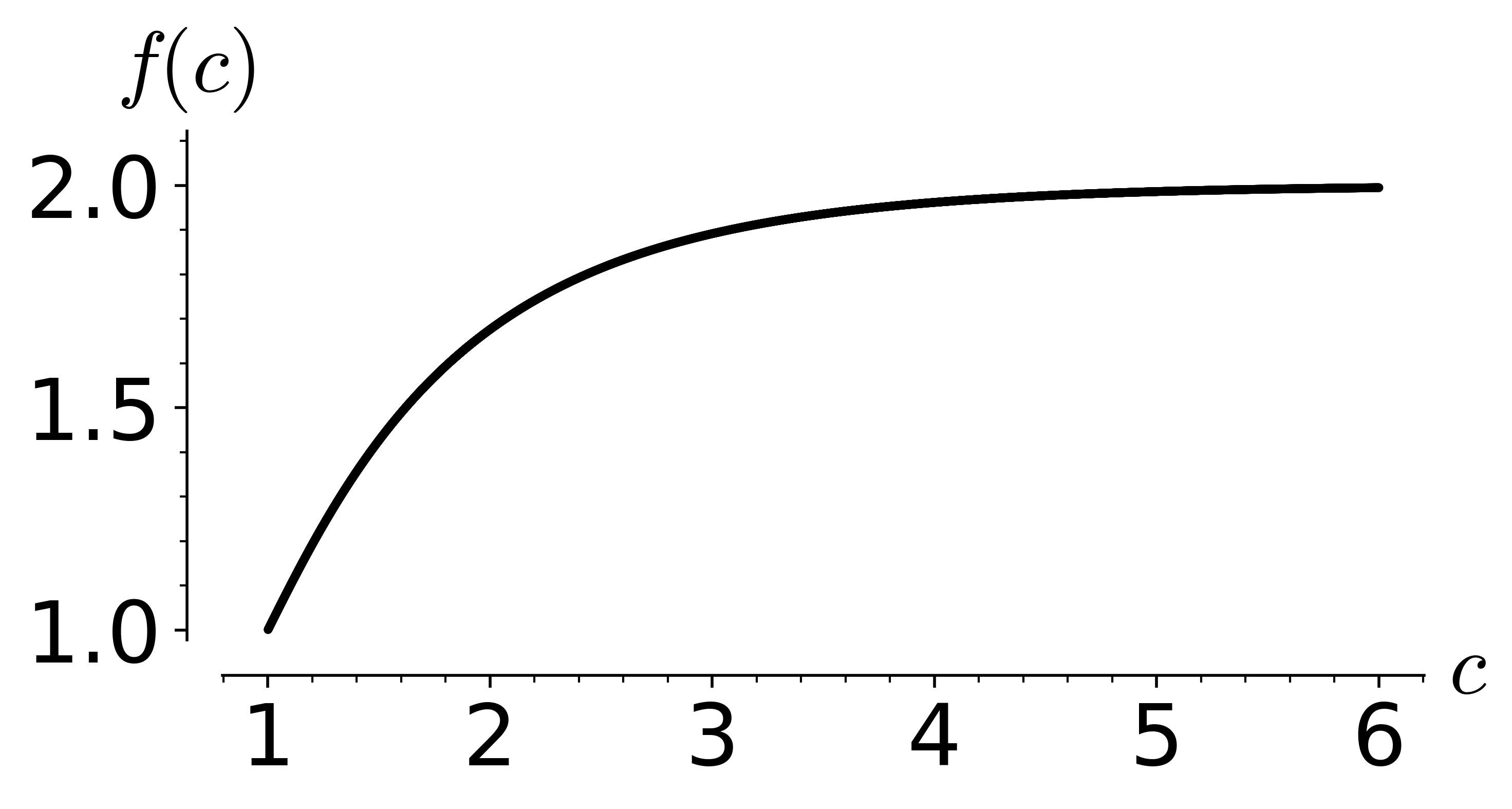
Given let be the unique positive solution of the equation and define
Denote by the inverse function of .
Note that is equal to the survival probability of a Galton-Watson process with offspring distribution Poisson with mean . Basic properties of the function , including the existence of the inverse function , can be found in A.1.
In the following theorem we provide the asymptotic order of the number of accepted edges when for any class of graphs satisfying the properties in Definition 1.4. As is ‘quite close’ to in this early stage of the evolution, it is more convenient to state the asymptotic order of the number of rejected edges instead of .
Theorem 1.7.
Let be a class of graphs satisfying the properties (a)–(f) in Definition 1.4 and be the -constrained random graph process. Let be a function which tends to arbitrarily slowly as . Let and . Then whp

When for , the statement that whp can be equivalently formulated as follows: For each there exists a such that for all sufficiently large , i.e., the statement is ‘slightly weaker’ than having whp .
In the case for the statement that whp can be simplified to whp . Using 1.7 we obtain the following nice, alternative description of a -constrained random graph process: In the very early stage of the process when , ‘almost’ all edges are accepted. More formally, whp the ‘next’ edge will be accepted as long as . However, this changes when for : The acceptance mainly depends whether or not both of the endpoints of lie in the largest component of .
Corollary 1.8.
Let be a class of graphs satisfying the properties (a)–(f) in Definition 1.4 and be the -constrained random graph process. Let be such that for a constant , and let denote the largest component of . Then whp the following hold.
- (a)
If , then is rejected.
- (b)
If , then is accepted.
Using 1.7 we can determine the asymptotic number of queried edges until of them have been accepted in the case for . In particular, this answers the open problem on for the property of being planar from [13].
Corollary 1.9.
Let be a class of graphs satisfying the properties (a)–(f) in Definition 1.4 and be as defined in (2). If for a constant , then whp
In particular, whp , where .
We note that 1.9 follows directly from 1.7 and the observation that is strictly increasing (see A.1(b)).
Our next main result provides the asymptotic order of the largest component of .
Theorem 1.10.
Let be a class of graphs satisfying the properties (a)–(f) in Definition 1.4 and be the -constrained random graph process. Let and . Let be defined as in (1) and let denote the number of vertices in the largest component of . Then whp
For the property of being planar 1.10 reveals a different behaviour of in the ‘sparse’ regime than that of the uniform random planar graph . More formally, if for , then whp
| (3) |
where the last equality follows from [18]. We refer to Figure 2 for an illustration of and .


1.3. Outline of the paper
2. Preliminaries
2.1. Notations for graphs
We begin with some notations for graphs that will be used in the rest of the paper.
Definition 2.1.
Given a graph we denote by
- •
the vertex set of and
-
the order of , i.e., the number of vertices in ;
- •
the edge set of and
-
the size of , i.e., the number of edges in ;
- •
the maximum degree of ;
- •
the largest component of ;
- •
the 2-core of , which is the maximal subgraph of with minimum degree at least two;
- •
the excess of , where is the number of tree components in .
Definition 2.2.
Given a class of graphs, we write for the subclass of containing the graphs on vertex set and for the subclass of containing the graphs on vertex set with edges, respectively.
2.2. Properties of the Erdős-Rényi random graph
In this section we state the properties of the Erdős-Rényi random graph which we will use in our proofs. First we consider the case for and then the case for .
Theorem 2.3 ([4, 22, 23, 26]).
Let and be such that for and be the largest component of the Erdős-Rényi random graph . Furthermore, let be the 2-core of and be the forest obtained from by deleting the edges of . Then whp
- (a)
;
- (b)
;
- (c)
each tree component of is of order ;
- (d)
;
- (e)
if in addition .
We note that (a) and (b) are shown in [22], (d) in [4], and (e) in [23], respectively. Furthermore, (c) follows by the fact from [26] that conditioned on fixed values of and , whp all tree components of are of order as long as . Furthermore, whp satisfies this condition, because whp by [23] and by (a).
Next we collect some properties of the Erdős-Rényi random graph when for .
Theorem 2.4 ([9]).
Let be such that for . Let be the Erdős-Rényi random graph, and the largest component of . Furthermore, let and be as in Definition 1.6. Then whp
- (a)
;
- (b)
all components of apart from are of order ;
- (c)
.
2.3. Properties of and
We will often use the following simple observation.
Remark 2.5.
Due to properties (b) and (e) of Definition 1.4 there is a path between two vertices in if and only if there is one in .
Next, we show that the number of rejected edges up to step is bounded above by the excess of . This will be a main ingredient to obtain the upper bounds in 1.7.
Lemma 2.6.
For all we have
Proof.
We consider an edge which is rejected in the -constrained random graph process. By Definition 1.4(e) and (f) the two endpoints of lie in the same component of , which is not a tree component. Together with the fact it implies that adding to increases the excess by one, i.e., . As is non-decreasing in , this implies the statement. ∎
A graph class for which there exists a constant such that for all is often called small (see e.g., [24]). The following statement shows that the class in Definition 1.4 is small.
Theorem 2.7 ([24]).
Let be a class of graphs satisfying the properties (a), (c), and (d) in Definition 1.4. Then there exists a constant such that for all .
2.4. Decomposition of graphs
In the proof of 1.7 we will split the largest component of into connected parts of roughly equal size. To that end, we will use the following lemma, which is an extension of [20, Proposition 4.5] to vertex-weighted graphs.
Lemma 2.8.
Let be a connected graph with maximum degree at most . We assign each vertex a vertex-weight . Assume that for some . Then, given there exist disjoint vertex sets such that
- •
is connected for each ;
- •
for each ;
- •
,
where denotes the total vertex-weight of and the total vertex-weight of , respectively.
Proof.
We proceed by induction on . For let denote the single vertex in . We set if and let otherwise.
Now assume . If , we set . Assume otherwise that . We perform a breadth-first search (BFS) starting at some arbitrary vertex . For each vertex let be the set of vertices consisting of and all descendants of in the BFS-tree and let be the total vertex-weight of . Let be a vertex such that is minimal among all vertices with . We note that such a vertex exists, as . Let be the neighbours of that are contained in . By minimality of and the fact we have for all . Thus, we get . Therefore, we choose . By construction is connected and we have . Furthermore, the graph obtained from by deleting is connected and has less vertices than . Hence, we can apply the induction hypothesis to this graph to obtain the remaining sets of our desired decomposition. ∎
We will show that if we have a ‘suitable’ decomposition of , we cannot add too ‘many’ further edges without creating a minor of the complete graph for an appropriate . To that end, we will use the following lemma, which is a ‘weighted’ version of the well-known Turán’s theorem.
Lemma 2.9.
For fixed we assign a vertex-weight to each vertex of . Furthermore, we define the edge-weight for each edge . Let be the total vertex-weight of and be the maximum vertex-weight of . For each subgraph denote by the total edge-weight of . Then for each we have
Proof.
To ease notation, let . In [1] Bennett, English, and Talanda-Fisher showed that
where the maximum is taken over all partitions of into parts and denotes the total vertex-weight of . Now let be some partition for which the maximum is attained. Note that . Furthermore, we have
Using the ‘AM-QM inequality’, in other words, , we obtain
| (4) |
Finally, the total edge-weight of satisfies
This together with (4) implies the statement. ∎
3. Rejected edges: proof of 1.7
The upper bounds follow immediately from 2.6.
3.1. Proof of upper bounds
Before proving the lower bounds we first sketch the main ideas.
3.2. Proof idea for lower bounds
First we consider the case for . We use a consequence of the properties (a) and (d) in Definition 1.4 that there exists an such that no graph in contains the complete graph as a minor. We then apply a ‘sprinkling’ type argument: Let and let for . We first reveal the edges . Given the realisation of , we split the vertex set of the largest component of into disjoint sets of ‘almost’ equal sizes such that is connected for each , where . Next we reveal the remaining edges up to step and show that for each pair there are ‘many’ edges between and which are queried up to step . As is not a minor of , there are some pairs for which all of these edge are rejected. This provides a lower bound on the number of rejected edges. The precise way of decomposing the largest component of differs in the cases and . We note that it is sufficient to deal with these two cases, because the general case follows by considering appropriate subsequences.
The starting point for the case for is 2.7. Roughly speaking, it says that only a very small number of all graphs on vertices lie in . Using that we show that for each , whp there is no graph such that all edges of are already queried before step . In particular, this shows that whp . It is well known that whp and therefore also are connected. Thus, we obtain that whp . Furthermore, we have that
3.3. Proof of lower bounds
(i) We start with the case for .
Take and let , , , and . Furthermore, let and be the largest components of and , respectively.
Due to the properties (a) and (d) in Definition 1.4, there exists an such that there is no graph in having the complete graph as a minor. Now we distinguish two cases.
Case 1: . First reveal the edges .
Let be the 2-core of and the forest obtained from by deleting the edges of . Moreover, for a vertex let be the tree component of containing . By Definition 1.4(b) and (e) we have and ; furthermore, each edge of is also contained in . Thus, there is a connected and spanning subgraph such that can be obtained by replacing each vertex in by the tree .
We apply 2.8 to , where we define the vertex-weight of a vertex by . Then due to 2.3(a), (c), and (e), whp the total vertex-weight of satisfies
the maximum vertex-weight of satisfies
and the maximum degree of is bounded by . Assuming this whp event holds, we apply 2.8 to with and and obtain disjoint vertex sets such that
- •
is connected for each ;
- •
for each ;
- •
,
where .
For let be the set of vertices that lie in some for a . Then are pairwise disjoint and satisfy the following properties:
- •
is connected for each ;
- •
for each ;
- •
.
Note that . Next we reveal the edges . We claim that whp for each pair there are at least many edges between points in and which have been queried up to step . Assume that for some this is not the case and let be such that . Then in the step of revealing there were at least many edges going between and which had not been queried yet. Hence, we have
Letting be the number of edges going between and that have been queried up to step it implies
| (5) |
As this shows the claim. By the choice of we know that is not a minor of . Hence, there is a pair such that there is no edge in going between and . Together with the claim this yields that whp at least many edges have been rejected up to step . This concludes the case .
Case 2: . First we reveal again only the edges .
Using 2.3(a) and (d) we have that whp and . Assuming this whp event holds, we apply 2.8 to where we assign a vertex-weight to each , , , and . This leads to disjoint sets such that is connected for each ,
| (6) | ||||
| (7) |
Next reveal the remaining edges . We claim that whp for each pair there are at least edges that have been queried up to step . To prove the claim, let be fixed and denote by the number of edges between and that have been queried up to step . Analogous to (5) we obtain, with ,
where we used Chebyshev’s inequality, (6), and . As , the claim follows by the union bound. Next, let be the graph with (super)vertex set and two vertices and are connected if and only if there is an edge in going between and . We assign each vertex in the vertex-weight . Due to (6) and (7) we have that the maximum vertex-weight and the total vertex-weight of satisfy
Let be the set of unordered pairs such that there is no edge in going between and . We note that , as is not a minor of . Then by 2.9 we obtain
By definition of there is no edge in going between and for each unordered pair . Furthermore, whp for each of these pairs at least many edges between and have been queried up to step . Thus, the number of rejected edges satisfies that whp
This concludes the case and therefore also the case for .
(ii) We consider the case where for . Let , , and . We claim that whp
| (8) |
To show the claim, we use an idea from [13]: Let , , , , and as in Section 1.1 . We have
By 2.7 there exists a such that for all . Thus, we obtain by taking the union bound
which gives (8). Next we use the well-known fact that whp is connected (see e.g., [8]). By Remark 2.5 this is also true for . Together with (8) this implies that whp . As , we obtain whp . Due to we have . Hence, we have that whp
where we used 2.4(c) for the last equality. This shows the lower bound in the case for and concludes the proof of 1.7. ∎
4. Addable and forbidden edges and proof of 1.8
How likely is it that the ‘next’ edge gets accepted? Equivalently, what is the number of potential edges that can be added to without violating property ?
Definition 4.1.
Let be a class of graphs and let . Then we call an edge addable to if and forbidden in otherwise, i.e., if . Furthermore, we set
In the next theorem we determine the number of forbidden edges in . Combining it with 1.7 one can also compute , because
Theorem 4.2.
Let be a class of graphs satisfying the properties (a)–(f) in Definition 1.4 and be the -constrained random graph process. Let be a function which tends to arbitrarily slowly as . Let and . Then whp
We note that for planar graphs (and many other graph classes mentioned in 1.5) we actually have that whp
However, this is not true in general for a class that satisfies the properties (a)–(f) in Definition 1.4. In order to prove 4.2, we will use the following lemma. We recall that for fixed we denote by the number of rejected edges up to step .
Lemma 4.3.
Let and be as in 4.2. Let and be such that and .
- (a)
If whp , then whp .
- (b)
If whp , then whp .
Proof.
Due to property (d) of Definition 1.4, a forbidden edge in stays forbidden in for all . Thus, is non-decreasing in . Let be fixed and we denote by the event that . Then we have that for each and large enough,
where we used in the last inequality. Hence, we obtain
Together with the fact that whp it implies that . As was arbitrary, statement (a) follows. Statement (b) can be obtained similarly. ∎
Proof of 4.2
(i) We start with the case for .
To prove the upper bound, we set . By 1.7 we have that whp . Hence, there exists such that and whp . Hence, 4.3(a) yields that whp
Similarly, we obtain the lower bound: Taking we have by 1.7 that whp and for , and thus . Together with 4.3(b) it implies that whp .
(ii) The assertions in the cases for and for can be shown similarly.
(iii) Finally, we consider the regime for . Let and . By 1.7 we have that whp
Hence, 4.3(a) implies that whp
With we obtain that whp
where we used A.1(a) in the last equality. Using 4.3(b) we obtain in a similar way that whp . This completes the proof. ∎
We conclude this section by showing 1.8.
Proof of 1.8
Let be the components of such that . By 2.4(a) and (b) and Remark 2.5 we have whp and . Furthermore, let be the subset of edges with both endpoints in and the remaining edges of . We have that whp
| (9) | ||||
| (10) |
Due to property (e) of Definition 1.4 the two endpoints of a forbidden edge lie in the same component. Hence, the number of forbidden edges in is whp at most
Together with (10) it shows assertion (b). Furthermore, it implies that the number of forbidden edges in is whp
5. The random graph : proof of 1.10
Throughout this section, let be a class of graphs satisfying the properties (a)–(f) in Definition 1.4 and be the -constrained random graph process. Recall that denotes the graph in which exactly edges have actually been added. We assume that is such that always exists, i.e., for any ordering of the potential edges, at least of them have been accepted at the end of the process.
Proof of 1.10
By Remark 2.5 we have and therefore we have that for
| (11) |
(i) First consider the case for . Let be small, , and . By 1.7 we have that whp . Thus, (11) implies that whp
where we used 2.4(a). As is continuous, we obtain with that whp .
(ii) The four cases where can be shown similarly.
(iii) Next, we observe that is non-decreasing in , , and . Thus, in case of the statement follows by taking in the previously shown fact that whp
if for .
Acknowledgement
The authors thank the anonymous referees for many helpful remarks to improve the presentation of this paper.
References
- [1] P. Bennett, S. English, and M. Talanda-Fisher. Weighted Turán problems with applications. Discrete Math., 342(8):2165–2172, 2019.
- [2] T. Bohman. The triangle-free process. Adv. Math., 221(5):1653–1677, 2009.
- [3] T. Bohman and P. Keevash. The early evolution of the -free process. Invent. Math., 181(2):291–336, 2010.
- [4] B. Bollobás. Vertices of given degree in a random graph. J. Graph Theory, 6(2):147–155, 1982.
- [5] B. Bollobás. Random graphs, volume 73 of Cambridge Studies in Advanced Mathematics. Cambridge University Press, Cambridge, second edition, 2001.
- [6] B. Bollobás and O. Riordan. Constrained graph processes. Electron. J. Combin., 7:Research Paper 18, 20, 2000.
- [7] V. E. Britikov. The structure of a random graph near a critical point. Diskret. Mat., 1(3):121–128, 1989.
- [8] P. Erdős and A. Rényi. On random graphs. I. Publ. Math. Debrecen, 6:290–297, 1959.
- [9] P. Erdős and A. Rényi. On the evolution of random graphs. Magyar Tud. Akad. Mat. Kutató Int. Közl., 5:17–61, 1960.
- [10] P. Erdős, S. Suen, and P. Winkler. On the size of a random maximal graph. In Proceedings of the Sixth International Seminar on Random Graphs and Probabilistic Methods in Combinatorics and Computer Science, “Random Graphs ’93” (Poznań, 1993), volume 6, pages 309–318, 1995.
- [11] G. Fiz Pontiveros, S. Griffiths, and R. Morris. The triangle-free process and the Ramsey number . Mem. Amer. Math. Soc., 263(1274):v+125, 2020.
- [12] A. Frieze and M. Karoński. Introduction to random graphs. Cambridge University Press, Cambridge, 2016.
- [13] S. Gerke, D. Schlatter, A. Steger, and A. Taraz. The random planar graph process. Random Structures Algorithms, 32(2):236–261, 2008.
- [14] O. Giménez and M. Noy. Asymptotic enumeration and limit laws of planar graphs. J. Amer. Math. Soc., 22(2):309–329, 2009.
- [15] S. Janson, D. E. Knuth, T. Łuczak, and B. Pittel. The birth of the giant component. Random Structures Algorithms, 4(3):231–358, 1993. With an introduction by the editors.
- [16] S. Janson, T. Łuczak, and A. Rucinski. Random graphs. Wiley-Interscience Series in Discrete Mathematics and Optimization. Wiley-Interscience, New York, 2000.
- [17] N. Kamčev, M. Krivelevich, N. Morrison, and B. Sudakov. The Kőnig graph process. Random Structures Algorithms, 57(4):1272–1302, 2020.
- [18] M. Kang and T. Łuczak. Two critical periods in the evolution of random planar graphs. Trans. Amer. Math. Soc., 364(8):4239–4265, 2012.
- [19] M. Krivelevich, M. Kwan, P.-S. Loh, and B. Sudakov. The random -matching-free process. Random Structures Algorithms, 53(4):692–716, 2018.
- [20] M. Krivelevich and A. Nachmias. Coloring complete bipartite graphs from random lists. Random Structures Algorithms, 29(4):436–449, 2006.
- [21] M. Krivelevich, B. Sudakov, and D. Vilenchik. On the random satisfiable process. Combin. Probab. Comput., 18(5):775–801, 2009.
- [22] T. Łuczak. Component behavior near the critical point of the random graph process. Random Structures Algorithms, 1(3):287–310, 1990.
- [23] T. Łuczak. Cycles in a random graph near the critical point. Random Structures Algorithms, 2(4):421–439, 1991.
- [24] S. Norine, P. Seymour, R. Thomas, and P. Wollan. Proper minor-closed families are small. J. Combin. Theory Ser. B, 96(5):754–757, 2006.
- [25] D. Osthus and A. Taraz. Random maximal -free graphs. Random Structures Algorithms, 18(1):61–82, 2001.
- [26] J. L. Pavlov. The asymptotic distribution of the maximum size of trees in a random forest. Teor. Verojatnost. i Primenen., 22(3):523–533, 1977.
- [27] N. Robertson and P. D. Seymour. Graph minors. VIII. A Kuratowski theorem for general surfaces. J. Combin. Theory Ser. B, 48(2):255–288, 1990.
- [28] A. Ruciński and N. C. Wormald. Random graph processes with degree restrictions. Combin. Probab. Comput., 1(2):169–180, 1992.
- [29] A. Ruciński and N. C. Wormald. Random graph processes with maximum degree . Ann. Appl. Probab., 7(1):183–199, 1997.
Appendix A Properties of
Lemma A.1.
For let be the unique positive solution of the equation and let (as in Definition 1.6). Then the following hold:
- (a)
;
- (b)
is strictly increasing;
- (c)
is continuous;
- (d)
;
- (e)
;
- (f)
is bijective and therefore, has an inverse .
Proof.