The Rescaled Pólya Urn and the Wright-Fisher process with mutation

Giacomo Aletti and Irene Crimaldi Note: ADAMSS Center, Università degli Studi di Milano, Milan, Italy, giacomo.aletti@unimi.it Note: IMT School for Advanced Studies, Lucca, Italy, irene.crimaldi@imtlucca.it

Abstract

In [2, 3] the authors introduce, study and apply a new variant of the Eggenberger-Pólya urn, called the “Rescaled” Pólya urn, which, for a suitable choice of the model parameters, is characterized by the following features: (i) a “local” reinforcement, i.e. a reinforcement mechanism mainly based on the last observations, (ii) a random persistent fluctuation of the predictive mean, and (iii) a long-term almost sure convergence of the empirical mean to a deterministic limit, together with a chi-squared goodness of fit result for the limit probabilities. In this work, motivated by some empirical evidences in [3], we show that the multidimensional Wright-Fisher diffusion with mutation can be obtained as a suitable limit of the predictive means associated to a family of rescaled Pólya urns.

Keywords: Pólya urn; predictive mean; urn model; Wright-Fisher diffusion.

1 Introduction

The standard Eggenberger-Pólya urn [11, 22] has been widely studied and generalized. In its simplest form, this model with $k$ -colors works as follows. An urn contains $N_{0\,i}$ balls of color $i$ , for $i=1,\dots,k$ , and, at each time-step, a ball is extracted from the urn and then it is returned inside the urn together with $\alpha>0$ additional balls of the same color. Therefore, if we denote by $N_{n\,i}$ the number of balls of color $i$ in the urn at time-step $n$ , we have

N_{n\,i}=N_{n-1\,i}+\alpha\xi_{n\,i}\qquad\mbox{for }n\geq 1,

where $\xi_{n\,i}=1$ if the extracted ball at time-step $n$ is of color $i$ , and $\xi_{n\,i}=0$ otherwise. The parameter $\alpha$ regulates the reinforcement mechanism: the greater $\alpha$ , the greater the dependence of $N_{n\,i}$ on $\sum_{h=1}^{n}\xi_{h\,i}$ .
In [1, 2, 3] the Rescaled Pólya (RP) urn has been introduced, studied, generalized and applied. This model is characterized by the introduction of a parameter $\beta$ in the original model so that

	$\displaystyle N_{n\,i}$	$\displaystyle=b_{i}+B_{n\,i}$		$\displaystyle\text{with }$
	$\displaystyle B_{n+1\,i}$	$\displaystyle=\beta B_{n\,i}+\alpha\xi_{n+1\,i}$		$\displaystyle n\geq 0.$

Therefore, the urn initially contains $b_{i}+B_{0\,i}>0$ balls of color $i$ and the parameter $\beta\geq 0$ , together with $\alpha>0$ , regulates the reinforcement mechanism. More precisely, the term $\beta B_{n\,i}$ links $N_{n+1\,i}$ to the “configuration” at time-step $n$ through the “scaling” parameter $\beta$ , and the term $\alpha\xi_{n+1\,i}$ links $N_{n+1\,i}$ to the outcome of the extraction at time-step $n+1$ through the parameter $\alpha$ . The case $\beta=1$ obviously corresponds to the standard Eggenberger-Pólya urn with an initial number $N_{0\,i}=b_{i}+B_{0\,i}$ of balls of color $i$ . When $\beta<1$ , the RP urn model exhibits the following three features:

(i)

a “local” reinforcement, i.e. a reinforcement mechanism mainly based on the last observations;
(ii)

a random persistent fluctuation of the predictive mean $\psi_{n\,i}=E[\xi_{n+1\,i}=1|\,\xi_{h\,j},\,0\leq h\leq n,\,1\leq j\leq k]$ ;
(iii)

a long-term almost sure convergence of the empirical mean $\sum_{n=1}^{N}\xi_{n\,i}/N$ to the deterministic limit $p_{i}=b_{i}/\sum_{i=1}^{n}b_{i}$ , and a chi-squared goodness of fit result for the long-term probability distribution $\{p_{1},\dots,p_{k}\}$ .

Regarding point (iii), we specifically have that the chi-squared statistics

\chi^{2}=N\sum_{i=1}^{k}\frac{(O_{i}/N-p_{i})^{2}}{p_{i}},

where $N$ is the size of the sample and $O_{i}=\sum_{n=1}^{N}\xi_{n\,i}$ the number of observations equal to $i$ in the sample, is asymptotically distributed as $\chi^{2}(k-1)\lambda$ , with $\lambda>1$ . This means that the presence of correlation among observations mitigates the effect of the sample size $N$ , that multiplies the chi-squared distance between the observed frequencies and the expected probabilities. This aspect is important for the statistical applications in the context of a “big sample”, when a small value of the chi-squared distance might be significant, and hence a correction related to the correlation between observations is desirable. In [1, 2] it is described a possible application in the context of clustered data, with independence between clusters and correlation, due to a reinforcement mechanism, inside each cluster.
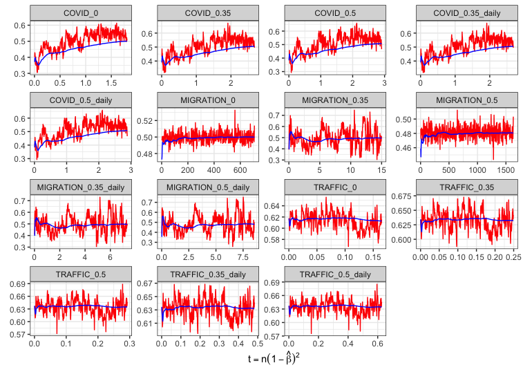
In [3] the RP urn has been applied as a good model for the evolution of the sentiment associated to Twitter posts. For these processes the estimated values of $\beta$ are strictly smaller than $1$ , but very near to $1$ . Note that the RP urn dynamics with such a value for $\beta$ cannot be approximated by the standard Pólya urn ( $\beta=1$ ), because one would loose the fluctuations of the predictive means and the possibility of touching the barriers $\{0,1\}$ . In Figure 1, we show the plots of the processes $(\psi_{n\,1})_{n}$ and $(\bar{\xi}_{n\,1})_{n}$ , reconstructed from the data and rescaled in time as $t=n(1-\beta)^{2}$ . (Details about the analyzed data sets, the reconstruction process and the parameters estimation can be found in [3].) In this work, we show that the law of such processes can be approximated by the one of the Wright-Fisher diffusion with mutation. More precisely, we prove that the multidimensional Wright-Fisher diffusion with mutation can be obtained as a suitable limit of the predictive means associated to a family of RP urns with $\beta\in$ [0,1) $,\beta\to 1$ .

Refer to caption — Figure 1: Twitter data: In [3] the RP urn has been proven to be a good model for the evolution of the sentiment associated to Twitter posts. For these processes we have estimated values of $\beta$ smaller than $1$ , but very near to $1$ . We here plot the processes $(\psi_{n\,1})_{n}$ (red color) and $(\bar{\xi}_{n\,1})_{n}$ (blue color), reconstructed from the data and rescaled in time as $t=n(1-\beta)^{2}$ . Details about the analyzed data sets, the reconstruction process and the estimated parameters can be found in [3].

The Wright–Fisher (WF) class of diffusion processes models the evolution of the relative frequency of a genetic variant, or allele, in a large randomly mating population with a finite number $k$ of genetic variants. When $k=2$ , the WF diffusion obeys the one-dimensional stochastic differential equation

dX_{t}=F(X_{t})dt+\sqrt{X_{t}(1-X_{t})}dW_{t},\qquad X_{0}=x_{0},t\in[0,T].

(1)

The drift coefficient, $F:[0,1]\to R$ , can include a variety of evolutionary forces such as mutation and selection. For example, $F(x)=p_{1}-(p_{1}+p_{2})x=p_{1}(1-x)-p_{2}x$ describes a process with recurrent mutation between the two alleles, governed by the mutation rates $p_{1}>0$ and $p_{2}>0$ . The drift vanishes when $x=p_{1}/(p_{1}+p_{2})$ which is an attracting point for the dynamics. Equation (1) can be generalized to the case $k>2$ . The WF diffusion processes are widely employed in Bayesian Statistics, as models for time-evolving priors [12, 14, 24, 28] and as a dicrete-time finite-population construction method of the two-parameter Poisson-Dirichlet diffusion [6]. They have been applied in genetics [4, 16, 23, 26, 29, 31], in biophysics [7, 8], in filtering theory [5, 25] and in finance [9, 13].
The benefit coming from the proven limit result is twofold. First, the known properties of the WF process can give a description of the RP urn when the parameter $\beta$ is strictly smaller than one, but very near to one. Second, the given result might furnish the theoretical base for a new simulation method of the WF process. Indeed, simulation from Equation (1) is highly nontrivial because there is no known closed form expression for the transition function of the diffusion, even in the simple case with null drift [18].
The sequel of the paper is so structured. In Section 2 we set up our notation and we formally define the RP urn model. Section 3 provides the main result of this work, that is the convergence result of a suitable family of predictive means associated to RP urns with $\beta\to 1$ . In Section 4 we list some properties of the considered stochastic processes. In particular, we recall some properties of the WF diffusion with mutation, connecting them to the parameters of the RP urn model. Section 5 focuses on the case $k=2$ . Finally, in Section 6 we introduce the notion of dominant component (color in the RP urn), related to the possibility of reaching the barrier $1$ . The paper closes with two technical appendices.

2 The Rescaled Pólya urn

In all the sequel (unless otherwise specified) we suppose given two parameters $\alpha>0$ and $\beta\geq 0$ . Given a vector ${\boldsymbol{x}}=(x_{1},\ldots,x_{k})^{\top}\in\mathbb{R}^{k}$ , we set $|{\boldsymbol{x}}|=\sum_{i=1}^{k}|x_{i}|$ and $\|{\boldsymbol{x}}\|^{2}={\boldsymbol{x}}^{\top}{\boldsymbol{x}}=\sum_{i=1}^{k}|x_{i}|^{2}$ . Moreover we denote by ${\boldsymbol{1}}$ and ${\boldsymbol{0}}$ the vectors with all the components equal to $1$ and equal to $0$ , respectively.

To formally work with the RP urn model presented in the introduction, we add here some notations. In the whole sequel the expression “number of balls” is not to be understood literally, but all the quantities are real numbers, not necessarily integers. The urn initially contains $b_{i}+B_{0\,i}>0$ distinct balls of color $i$ , with $i=1,\dots,k$ . We set ${\boldsymbol{b}}=(b_{1},\dots,b_{k})^{\top}$ and ${\boldsymbol{B_{0}}}=(B_{0\,1},\dots,B_{0\,k})^{\top}$ . In all the sequel (unless otherwise specified) we assume $|{\boldsymbol{b}}|>0$ and we set ${\boldsymbol{p}}=\frac{{\boldsymbol{b}}}{|{\boldsymbol{b}}|}$ . At each time-step $(n+1)\geq 1$ , a ball is drawn at random from the urn, obtaining the random vector ${\boldsymbol{\xi_{n+1}}}=(\xi_{n+1\,1},\ldots,\xi_{n+1\,k})^{\top}$ defined as

\xi_{n+1\,i}=\begin{cases}1&\text{when the extracted ball at time $n+1$ is of color $i$}\\ 0&\text{otherwise},\end{cases}

and the number of balls in the urn is so updated:

{\boldsymbol{N_{n+1}}}={\boldsymbol{b}}+{\boldsymbol{B_{n+1}}}\qquad\text{with}\qquad{\boldsymbol{B_{n+1}}}=\beta{\boldsymbol{B_{n}}}+\alpha{\boldsymbol{\xi_{n+1}}}\,,

(2)

which gives

{\boldsymbol{B_{n}}}=\beta^{n}{\boldsymbol{B_{0}}}+\alpha\beta^{n}\sum_{h=1}^{n}\beta^{-h}{\boldsymbol{\xi_{h}}}\,.

(3)

Similarly, from the equality

|{\boldsymbol{B_{n+1}}}|=\beta|{\boldsymbol{B_{n}}}|+\alpha\,,

we get, using $\sum_{h=0}^{n-1}x^{h}=(1-x^{n})/(1-x)$ ,

|{\boldsymbol{B_{n}}}|=\beta^{n}|{\boldsymbol{B_{0}}}|+\alpha\sum_{h=1}^{n}\beta^{n-h}=\beta^{n}\left(|{\boldsymbol{B_{0}}}|-\frac{\alpha}{1-\beta}\right)+\frac{\alpha}{1-\beta}\,.

(4)

Setting $r^{*}_{n}=|{\boldsymbol{N_{n}}}|=|{\boldsymbol{b}}|+|{\boldsymbol{B_{n}}}|$ , that is the total number of balls in the urn at time-step $n$ , we get the relations

r_{n+1}^{*}=r_{n}^{*}+(\beta-1)|{\boldsymbol{B_{n}}}|+\alpha

(5)

and

r_{n}^{*}=|{\boldsymbol{b_{0}}}|+\frac{\alpha}{1-\beta}+\beta^{n}\left(|{\boldsymbol{B_{0}}}|-\frac{\alpha}{1-\beta}\right).

(6)

Moreover, setting $\mathcal{F}_{0}$ equal to the trivial $\sigma$ -field and $\mathcal{F}_{n}=\sigma({\boldsymbol{\xi_{1}}},\dots,{\boldsymbol{\xi_{n}}})$ for $n\geq 1$ , the conditional probabilities ${\boldsymbol{\psi_{n}}}=(\psi_{n\,1},\ldots,\psi_{n\,k})^{\top}$ of the extraction process, also called predictive means, are

{\boldsymbol{\psi_{n}}}=E[{\boldsymbol{\xi_{n+1}}}|\mathcal{F}_{n}]=\frac{{\boldsymbol{N_{n}}}}{|{\boldsymbol{N_{n}}}|}=\frac{{\boldsymbol{b}}+{\boldsymbol{B_{n}}}}{r_{n}^{*}}\qquad n\geq 0

(7)

and, from (3) and (4), we have

{\boldsymbol{\psi_{n}}}=\frac{{\boldsymbol{b}}+\beta^{n}{\boldsymbol{B_{0}}}+\alpha\sum_{h=1}^{n}\beta^{n-h}{\boldsymbol{\xi_{h}}}}{|{\boldsymbol{b}}|+\frac{\alpha}{1-\beta}+\beta^{n}\left(|{\boldsymbol{B_{0}}}|-\frac{\alpha}{1-\beta}\right)}\,.

(8)

The dependence of ${\boldsymbol{\psi_{n}}}$ on ${\boldsymbol{\xi_{h}}}$ depends on the factor $f(h,n)=\alpha\beta^{n-h}$ , with $1\leq h\leq n,\,n\geq 0$ . In the case of the standard Eggenberger-Pólya urn, that corresponds to $\beta=1$ for all $n$ , each observation ${\boldsymbol{\xi_{h}}}$ has the same “weight” $f(h,n)=\alpha$ . Instead, when $\beta<1$ the factor $f(h,n)$ increases with $h$ , then the main contribution is given by the most recent extractions. We refer to this phenomenon as “local” reinforcement. The case $\beta=0$ is an extreme case, for which ${\boldsymbol{\psi_{n}}}$ depends only on the last extraction ${\boldsymbol{\xi_{n}}}$ .
By means of (7), together with (2) and (5), we get

{\boldsymbol{\psi_{n+1}}}-{\boldsymbol{\psi_{n}}}=-\frac{(1-\beta)}{r_{n+1}^{*}}|{\boldsymbol{b}}|\big({\boldsymbol{\psi_{n}}}-{\boldsymbol{p}}\big)+\frac{\alpha}{r_{n+1}^{*}}\big({\boldsymbol{\xi_{n+1}}}-{\boldsymbol{\psi_{n}}}\big).

(9)

Setting $\Delta{\boldsymbol{M_{n+1}}}={\boldsymbol{\xi_{n+1}}}-{\boldsymbol{\psi_{n}}}$ and letting $\epsilon_{n}=|{\boldsymbol{b}}|(1-\beta)/r_{n+1}^{*}$ and $\delta_{n}=\alpha/r_{n+1}^{*}$ , from (9) we obtain

{\boldsymbol{\psi_{n+1}}}-{\boldsymbol{\psi_{n}}}=-\epsilon_{n}({\boldsymbol{\psi_{n}}}-{\boldsymbol{p}})+\delta_{n}\Delta{\boldsymbol{M_{n+1}}}\,.

(10)

3 Main result

Consider the RP urn with parameters $\alpha>0$ , $\beta\in[0,1)$ and ${\boldsymbol{B_{0}}}$ such that $|{\boldsymbol{B_{0}}}|=r(\beta)=\alpha/(1-\beta)$ and set $b=|{\boldsymbol{b}}|>0$ . Consequently, the total number of balls in the urn along the time-steps is constantly equal to $r^{*}(\beta)=b+r(\beta)$ and, if we denote by ${\boldsymbol{\psi^{(\beta)}}}=({\boldsymbol{\psi_{n}^{(\beta)}}})_{n}$ the predictive means corresponding to the fixed value $\beta$ , we have the dynamics

{\boldsymbol{\psi^{(\beta)}_{n}}}-{\boldsymbol{\psi^{(\beta)}_{n-1}}}=-\epsilon(\beta)\big({\boldsymbol{\psi^{(\beta)}_{n-1}}}-{\boldsymbol{p}}\big)+\delta(\beta)\Delta{\boldsymbol{M_{n}^{(\beta)}}}\,,

(11)

where

\epsilon(\beta)=\frac{b(1-\beta)^{2}}{\alpha+b(1-\beta)},\qquad\delta(\beta)=\frac{\alpha(1-\beta)}{\alpha+b(1-\beta)}

(12)

and ${\boldsymbol{\Delta M_{n}^{(\beta)}}}={\boldsymbol{\xi^{(\beta)}_{n}}}-{\boldsymbol{\psi^{(\beta)}_{n-1}}}$ . (Note that we have $\epsilon(\beta)\sim c\delta(\beta)^{2}$ for $\beta\to 1$ , with $c=b/\alpha>0$ .) Finally, define ${{\boldsymbol{X}}^{(\beta)}}=({\boldsymbol{X_{t}^{(\beta)}}})_{t\geq 0}$ where

{\boldsymbol{X^{(\beta)}_{t}}}={\boldsymbol{\psi^{(\beta)}_{\lfloor t/(1-\beta)^{2}\rfloor}}}\quad\iff\quad{\boldsymbol{X^{(\beta)}_{t}}}={\boldsymbol{\psi^{(\beta)}_{n-1}}},\ t\in[\,(n-1)(1-\beta)^{2},n(1-\beta)^{2}\,).

(13)

The following result holds true:

Theorem 1.

Suppose that ${\boldsymbol{X^{(\beta)}_{0}}}$ weakly converges towards some process ${\boldsymbol{X_{0}}}$ when $\beta\to 1$ . Then, for $\beta\to 1$ , the family of stochastic processes $\{{\boldsymbol{X^{(\beta)}}},\,\beta\in[0,1)\}$ weakly converges towards the $k$ -alleles Wright-Fisher diffusion ${\boldsymbol{X}}=({\boldsymbol{X_{t}}})_{t\geq 0}$ , with type-independent mutation kernel given by ${\boldsymbol{p}}$ and dynamics

d{\boldsymbol{X_{t}}}=-b\frac{{\boldsymbol{X_{t}}}-{\boldsymbol{p}}}{\alpha}dt+\Sigma({\boldsymbol{X_{t}}})d{\boldsymbol{W_{t}}},

(14)

with $\Sigma({\boldsymbol{X_{t}}})\Sigma({\boldsymbol{X_{t}}})^{\top}=\Big(\mathrm{diag}({\boldsymbol{X_{t}}})-{\boldsymbol{X_{t}}}{\boldsymbol{X_{t}}}^{\top}\Big)$ and ${\boldsymbol{1}}^{\top}\Sigma({\boldsymbol{X_{t}}})={\boldsymbol{0}}^{\top}$ , that is

\displaystyle\Sigma({\boldsymbol{X_{t}}})_{ij}=\begin{cases}0&\text{if $X_{t,i}X_{t,j}=0$ or $i<j$}\\ \sqrt{X_{t,i}\frac{\sum_{l=i+1}^{k}X_{t,l}}{\sum_{l=i}^{k}X_{t,l}}}&\text{if $i=j$ and $X_{t,i}X_{t,j}\neq 0$}\\ -X_{t,i}\sqrt{\frac{X_{t,j}}{\sum_{l=j}^{k}X_{t,l}\sum_{l=j+1}^{k}X_{t,l}}}&\text{if $i>j$ and $X_{t,i}X_{t,j}\neq 0$.}\end{cases}

(15)

Proof.

Fix a sequence $(\beta_{n})$ , with $\beta_{n}\in[0,1)$ and $\beta_{n}\to 1$ . The sequence of processes $\{{\boldsymbol{X^{(\beta_{n})}}},\,n\in\mathbb{N}\}$ is bounded, and hence we have to prove the tighthness of the sequence in the space $D^{k}[0,\infty)$ of right-continuous functions with the ususal Skorohod topology, and the characterization of the law of the unique limit process.

For any $f\in C^{2}_{b}$ , define

$\displaystyle\gamma_{n}^{(\beta,f)}({\boldsymbol{x}})$	$\displaystyle=\widehat{A}^{(\beta)}f((n-1)(1-\beta)^{2})({\boldsymbol{x}})$	(16)
	$\displaystyle=E\Big[\frac{f({\boldsymbol{X^{(\beta)}_{n(1-\beta)^{2}}}})-f({\boldsymbol{X^{(\beta)}_{(n-1)(1-\beta)^{2}}}})}{(1-\beta)^{2}}\Big\|{\boldsymbol{X^{(\beta)}_{(n-1)(1-\beta)^{2}}}}={\boldsymbol{x}}\Big]$
	$\displaystyle=E\Big[\frac{f({\boldsymbol{\psi^{(\beta)}_{n}}})-f({\boldsymbol{\psi^{(\beta)}_{n-1}}})}{(1-\beta)^{2}}\Big\|{\boldsymbol{\psi^{(\beta)}_{n-1}}}={\boldsymbol{x}}\Big]$
	$\displaystyle\mathop{=}^{\text{by \eqref{dinamica-psinEps}}}\frac{1}{(1-\beta)^{2}}\bigg(E\Big[f({\boldsymbol{x}})+\sum_{i}\frac{\partial f}{\partial x_{i}}({\boldsymbol{x}})(-\epsilon(\beta)(x_{i}-{p_{i}})+\delta(\beta)\Delta{M_{n,i}}^{(\beta)})$
	$\displaystyle+\tfrac{1}{2}\delta(\beta)^{2}\sum_{ij}\frac{\partial^{2}f}{\partial x_{i}\partial x_{j}}({\boldsymbol{x}})\Delta M_{n,i}^{(\beta)}\Delta M_{n,j}^{(\beta)}+O((1-\beta)^{3})\Big\|\mathcal{F}_{n-1}\Big]-f({\boldsymbol{x}})\bigg)$
	$\displaystyle=-\tfrac{b}{\alpha+b(1-\beta)}\sum_{i}\frac{\partial f}{\partial x_{i}}({\boldsymbol{x}})(x_{i}-{p_{i}})+\frac{1}{2}\tfrac{\alpha^{2}}{(\alpha+b(1-\beta))^{2}}\sum_{ij}\frac{\partial^{2}f}{\partial x_{i}\partial x_{j}}({\boldsymbol{x}})(x_{i}{\mathbbm{1}}_{i=j}-x_{i}x_{j})$
	$\displaystyle+O(1-\beta)\,.$

We note that, for any $f\in C^{2}_{b}$ , the partial derivatives in (16) are uniformly dounded, as ${\boldsymbol{x}}$ belongs to the compact simplex $S=\{x_{i}\geq 0,\sum_{i}x_{i}=1\}$ . The family $\{\gamma_{n}^{(\beta,f)}({\boldsymbol{x}}),n\in\mathbb{N},\beta<1,{\boldsymbol{x}}\in S\}$ is then uniformly integrable. Thus, as a consequence of [20, Theorem 4] (or [21, ch. 7.4.3, Theorem 4.3, p. 236]), we have that the sequence of processes $\{{\boldsymbol{X^{(\beta_{n})}}},n\in\mathbb{N}\}$ is tight in the space of right-continuous functions with the ususal Skorohod topology. Since, for any $n$ and $t$ , ${\boldsymbol{X^{(\beta_{n})}_{t}}}\in S$ , then ${\boldsymbol{1}}^{\top}\Sigma({\boldsymbol{X_{t}}})={\boldsymbol{0}}^{\top}$ . Moreover, the generator of the limit process is determined by the limit

	$\displaystyle Af(t)({\boldsymbol{x}})$	$\displaystyle=\lim_{n\to\infty}\gamma_{\lfloor t/(1-\beta)^{2}\rfloor}^{(\beta_{n},f)}({\boldsymbol{x}})$
		$\displaystyle=-\tfrac{b}{\alpha}\sum_{i}\frac{\partial f}{\partial x_{i}}({\boldsymbol{x}})(x_{i}-{p_{i}})+\frac{1}{2}\sum_{ij}\frac{\partial^{2}f}{\partial x_{i}\partial x_{j}}({\boldsymbol{x}})(x_{i}{\mathbbm{1}}_{i=j}-x_{i}x_{j}).$

Hence, the weak limit of the sequence of the bounded processes ${\boldsymbol{X^{(\beta_{n})}}}$ is the diffusion process

d{\boldsymbol{X_{t}}}=-b\frac{{\boldsymbol{X_{t}}}-{\boldsymbol{p}}}{\alpha}dt+\Sigma({\boldsymbol{X_{t}}})d{\boldsymbol{W_{t}}},\qquad\Sigma({\boldsymbol{X_{t}}})\Sigma({\boldsymbol{X_{t}}})^{\top}=\Big(\mathrm{diag}({\boldsymbol{X_{t}}})-{\boldsymbol{X_{t}}}{\boldsymbol{X_{t}}}^{\top}\Big).

The expression (15) follows from [27, Corollary 3]. ∎

4 Some properties

We list here some properties.

4.1 Projections

Let ${\boldsymbol{J}}=\{J_{1},\ldots,J_{k_{J}}\}$ , be a partition of $\{1,\ldots,k\}$ , in that $J_{l}\neq\varnothing$ , $J_{i_{1}}\cap J_{i_{2}}=\varnothing$ , and $\cup_{l=1}^{k_{J}}=\{1,\ldots,k\}$ . Here $k_{j}$ denotes the cardinality of ${\boldsymbol{J}}$ . Define the $k_{J}$ -dimesional objects $({\boldsymbol{\psi^{(\beta,J)}_{n}}})_{n}$ , $({\boldsymbol{\xi^{(\beta,J)}_{n}}})_{n}$ and ${\boldsymbol{p^{(J)}}}$ as

\left.\begin{aligned} {\psi^{(\beta,{\boldsymbol{J}})}_{n,i}}&=\sum_{l\in J_{i}}{\psi^{(\beta)}_{n,l}}\\ {\xi^{(\beta,{\boldsymbol{J}})}_{n,i}}&=\sum_{l\in J_{l}}{\xi^{(\varepsilon)}_{n,l}}\\ {p_{i}^{({\boldsymbol{J}})}}&=\sum_{l\in J_{i}}{p_{l}}\end{aligned}\right\}\qquad\text{for }i=1,\ldots,k_{J},

and ${\boldsymbol{X^{(\beta,{\boldsymbol{J}})}_{t}}}={\boldsymbol{\psi^{(\beta,{\boldsymbol{J}})}_{\lfloor t/(1-\beta)^{2}\rfloor}}}$ . With these definitions, from (11), we immediately get that $({\boldsymbol{\psi^{(\beta,{\boldsymbol{J}})}_{n}}})_{n}$ is a $k_{J}$ -dimensional RP urn following the dynamics

{\boldsymbol{\psi^{(\beta,{\boldsymbol{J}})}_{n}}}-{\boldsymbol{\psi^{(\beta,{\boldsymbol{J}})}_{n-1}}}=-\epsilon(\beta)\big({\boldsymbol{\psi^{(\beta,{\boldsymbol{J}})}_{n-1}}}-{\boldsymbol{p^{(J)}}}\big)+\delta(\beta)\big({\boldsymbol{\xi^{(\beta,{\boldsymbol{J}})}_{n}}}-{\boldsymbol{\psi^{(\beta,{\boldsymbol{J}})}_{n-1}}}\big)

(17)

and that Theorem 1 holds for ${\boldsymbol{X^{(\beta,{\boldsymbol{J}})}_{t}}}$ . Consequently, the convergence to the Wright-Fisher diffusion still holds if we group together some components of the process. This property is summarized in the following theorem:

Theorem 2.

Under the hypothesis of Theorem 1, the process ${\boldsymbol{X^{(\beta,{\boldsymbol{J}})}_{t}}}$ weakly converges to ${\boldsymbol{X^{({\boldsymbol{J}})}_{t}}}$ which satisfy the SDE

d{\boldsymbol{X^{({\boldsymbol{J}})}_{t}}}=-b\frac{{\boldsymbol{X^{({\boldsymbol{J}})}_{t}}}-{\boldsymbol{p^{(J)}}}}{\alpha}dt+\Sigma({\boldsymbol{X^{({\boldsymbol{J}})}_{t}}})d{\boldsymbol{W^{*}_{t}}},

(18)

where ${\boldsymbol{W^{*}_{t}}}$ is a $k_{J}$ -dimensional standard Brownian motion, and $X^{({\boldsymbol{J}})}_{t,i}=\sum_{l\in J_{i}}X_{t,l}$ .

4.2 Limiting ergodic distribution

Since the simplex has dimension $k-1$ with respect to the Lebesgue measure, it is convenient to change the notations. Let $T^{k-1}$ be the $k-1$ -dimensional simplex defined by

T^{k-1}:=\{{\boldsymbol{y}}\in\mathbb{R}^{k-1}:y_{1}\geq 0,\ldots,y_{k-1}\geq 0,1-y_{1}-y_{2}-\cdots-y_{k-1}\geq 0\},

where, with the old definition, we have $x_{i}=y_{i},i<k$ and $x_{k}:=1-y_{1}-y_{2}-\cdots-y_{k-1}$ . Obviously, there is a one-to-one natural correspondence between $T^{k-1}$ and the simplex $\{{\boldsymbol{x}}\in\mathbb{R}^{k}:x_{1}\geq 0,\ldots,x_{k}\geq 0,\sum_{i}x_{i}=1\}$ defined by

{\boldsymbol{y}}=(y_{1},\ldots,y_{k-1})\quad\longleftrightarrow\quad(y_{1},\ldots,y_{k-1},1-y_{1}-y_{2}-\cdots-y_{k-1})=(x_{1},\ldots,x_{k-1},x_{k})={\boldsymbol{x}}.

The Markov diffusion process ${\boldsymbol{X_{t}}}$ in (14) may be ridefined as ${\boldsymbol{Y_{t}}}=(X_{t,1},\ldots,X_{t,k-1})$ on ${\boldsymbol{y}}\in T^{k-1}$ with the corresponding generator

Lf({\boldsymbol{y}})=-\tfrac{b}{\alpha}\sum_{i=1}^{k-1}\frac{\partial f}{\partial y_{i}}({\boldsymbol{y}})(y_{i}-{p_{i}})+\frac{1}{2}\sum_{i,j=1}^{k-1}\frac{\partial^{2}f}{\partial y_{i}\partial y_{j}}({\boldsymbol{y}})(y_{i}{\mathbbm{1}}_{i=j}-y_{i}y_{j}).

(19)

The Kolmogorov forward equation for the density $p({\boldsymbol{y}},t)$ of the limiting process ${\boldsymbol{Y}}_{t}$ is

\frac{\partial}{\partial t}p({\boldsymbol{y}},t)=\frac{1}{2}\bigg(\tfrac{b}{\alpha}\sum_{i=1}^{k-1}\frac{\partial}{\partial y_{i}}\Big(p({\boldsymbol{y}},t)(y_{i}-{p_{i}})\Big)\\ +\sum_{i=1}^{k-1}\frac{\partial^{2}}{\partial y_{i}^{2}}\Big(y_{i}(1-y_{i})p({\boldsymbol{y}},t)\Big)-2\sum_{1\leq i<j\leq k-1}\frac{\partial^{2}}{\partial y_{i}\partial y_{j}}\Big(y_{i}y_{j}p({\boldsymbol{y}},t)\Big)\bigg).

(20)

Therefore, it is not hard to show that the limit invariant ergodic distribution is

p({\boldsymbol{y}})=\frac{1}{B(2\tfrac{b}{\alpha}{\boldsymbol{p}})}(1-y_{1}-\cdots-y_{k-1})^{\frac{2b{(1-p_{1}-\cdots-p_{k-1})}}{\alpha}-1}\prod_{i=1}^{k-1}y_{i}^{\frac{2b{p_{i}}}{\alpha}-1},

(21)

because it satisfy (20) (see also [30]). The above distribution is the Dirichel distribution $\hbox{Dir}\big(2\frac{b}{\alpha}{\boldsymbol{p}}\big)$ as a function of ${\boldsymbol{x}}=({\boldsymbol{y}},1-y_{1}-\cdots-y_{k-1})$ .

4.3 Transition density of the limit process

The transition density $p({\boldsymbol{y_{0}}},{\boldsymbol{y}};t)$ is defined by

P({\boldsymbol{Y_{t}}}\in S|{\boldsymbol{Y_{0}}}={\boldsymbol{y_{0}}})=\int_{S\cap T^{k-1}}p({\boldsymbol{y_{0}}},{\boldsymbol{y}};t)d{\boldsymbol{y}}

and it can be represented in terms of series of orthogonal polynomials given in Appendix A. We first note that the limiting invariant ergoding distribution $p({\boldsymbol{y}})$ in (21) and the generator of the process ${\boldsymbol{Y_{t}}}$ in (19) may be rewritten on $T^{k-1}$ in terms of $\gamma_{i}=2\tfrac{b}{\alpha}p_{i}-1$ , obtaining

	$\displaystyle\pi_{\boldsymbol{\gamma}}({\boldsymbol{{y}}})$	$\displaystyle=\frac{1}{B(\boldsymbol{\gamma}+1)}\Big(\prod_{i=1}^{k-1}y_{i}^{\gamma_{i}}\Big)(1-y_{1}-y_{2}-\cdots-y_{k-1})^{\gamma_{k}}$
	$\displaystyle Lf({\boldsymbol{y}})$	$\displaystyle=-\tfrac{b}{\alpha}\sum_{i=1}^{k-1}\frac{\partial f}{\partial y_{i}}({\boldsymbol{y}})(y_{i}-{p_{i}})+\frac{1}{2}\sum_{i,j=1}^{k-1}\frac{\partial^{2}f}{\partial y_{i}\partial y_{j}}({\boldsymbol{y}})(y_{i}{\mathbbm{1}}_{i=j}-y_{i}y_{j})$
		$\displaystyle=\frac{1}{2}\bigg(\sum_{i=1}^{k-1}\Big(2\tfrac{b}{\alpha}p_{i}-\Big[\big(\sum_{i=1}^{k}2\tfrac{b}{\alpha}{p_{i}}-1\big)+k\Big]y_{i}\Big)\frac{\partial f}{\partial y_{i}}({\boldsymbol{y}})$
		$\displaystyle+\sum_{i=1}^{k-1}y_{i}(1-y_{i})\frac{\partial^{2}f}{\partial y_{i}^{2}}({\boldsymbol{y}})-2\sum_{1\leq i<j\leq k-1}y_{i}y_{j}\frac{\partial^{2}f}{\partial y_{i}\partial y_{j}}({\boldsymbol{y}})\bigg)$
		$\displaystyle=\frac{1}{2}\bigg(\sum_{i=1}^{k-1}\Big(\gamma_{i}+1-\Big[\big(\sum_{i=1}^{k}\gamma_{i}\big)+k\Big]y_{i}\Big)\frac{\partial f}{\partial y_{i}}({\boldsymbol{y}})$
		$\displaystyle+\sum_{i=1}^{k-1}y_{i}(1-y_{i})\frac{\partial^{2}f}{\partial y_{i}^{2}}({\boldsymbol{y}})-2\sum_{1\leq i<j\leq k-1}y_{i}y_{j}\frac{\partial^{2}f}{\partial y_{i}\partial y_{j}}({\boldsymbol{y}})\bigg).$

These two expressions coincide with those given in Appendix A. Let $\mathcal{V}_{n,\boldsymbol{\gamma}}$ be the space of orthogonal polynomials of degree $n$ as defined there and let $f^{\boldsymbol{\gamma}}_{{\mathbf{n}}}$ one of the three orthogonal bases given there. Then (22) implies

Lf^{\boldsymbol{\gamma}}_{{\mathbf{n}}}=\frac{1}{2}L_{\boldsymbol{\gamma}}f^{\boldsymbol{\gamma}}_{{\mathbf{n}}}=\frac{1}{2}(-\lambda_{n})f^{\boldsymbol{\gamma}}_{{\mathbf{n}}}=-\nu_{n}f^{\boldsymbol{\gamma}}_{{\mathbf{n}}},

where $\nu_{n}=\frac{n(n+k+\sum_{i=1}^{k}\gamma_{i})}{2}=\frac{n(n+2\tfrac{b}{\alpha}-1)}{2}$ . Note that each $\psi^{\boldsymbol{\gamma}}_{{\mathbf{n}}}(t,{\boldsymbol{y}})=e^{-\nu_{n}t}f^{\boldsymbol{\gamma}}_{{\mathbf{n}}}({\boldsymbol{y}})$ satisfies the Kolmogorov backward equation associated to the process ${\boldsymbol{Y_{t}}}$ , since

\frac{\partial}{\partial t}\psi^{\boldsymbol{\gamma}}_{{\mathbf{n}}}(t,{\boldsymbol{y}})=-\nu_{n}\psi^{\boldsymbol{\gamma}}_{{\mathbf{n}}}(t,{\boldsymbol{y}})=e^{-\nu_{n}t}Lf^{\boldsymbol{\gamma}}_{{\mathbf{n}}}({\boldsymbol{y}})=L\psi^{\boldsymbol{\gamma}}_{{\mathbf{n}}}(t,{\boldsymbol{y}}).

Now, for any ${\boldsymbol{y}}\in T^{k-1}$ , let $S_{{\boldsymbol{y}}}=\{{\boldsymbol{\bar{y}}}\colon 0\leq\bar{y}_{i}\leq y_{i},i=1,\ldots,k-1\}$ . The function

U_{{\boldsymbol{y}}}({\boldsymbol{y_{0}}},t)=P({\boldsymbol{Y_{t}}}\in{S_{{\boldsymbol{y}}}}|{\boldsymbol{Y_{0}}}={\boldsymbol{y_{0}}})=\int_{T^{k-1}}{\mathbbm{1}}_{S_{{\boldsymbol{y}}}}({\boldsymbol{\bar{y}}})p({\boldsymbol{y_{0}}},{\boldsymbol{\bar{y}}};t)d{\boldsymbol{\bar{y}}}

satisfies the Kolmogorov backward equation. As in [19, Section 15.13], we formally write $U_{{\boldsymbol{y}}}({\boldsymbol{y_{0}}},t)$ in terms of $\psi^{\boldsymbol{\gamma}}_{{\mathbf{n}}}(t,{\boldsymbol{y_{0}}})$ , since the Kolmogorov backward equation is additive, obtaining

U_{{\boldsymbol{y}}}({\boldsymbol{y_{0}}},t)=\sum_{n}\sum_{{\mathbf{n}}\colon n_{1}+\cdots+n_{k-1}=n}c_{\mathbf{n}}({\boldsymbol{y}})\psi^{\boldsymbol{\gamma}}_{{\mathbf{n}}}(t,{\boldsymbol{y_{0}}}).

Note that the boundary conditions imply that

	$\displaystyle{\mathbbm{1}}_{S_{{\boldsymbol{y}}}}({\boldsymbol{{y_{0}}}})$	$\displaystyle=\lim_{t\to 0^{+}}U_{{\boldsymbol{y}}}({\boldsymbol{y_{0}}},t)=\lim_{t\to 0^{+}}\sum_{n}\sum_{{\mathbf{n}}\colon n_{1}+\cdots+n_{k-1}=n}c_{\mathbf{n}}({\boldsymbol{y}})e^{-\nu_{n}t}f^{\boldsymbol{\gamma}}_{{\mathbf{n}}}({\boldsymbol{y_{0}}})$
		$\displaystyle=\sum_{n}\sum_{{\mathbf{n}}\colon n_{1}+\cdots+n_{k-1}=n}c_{\mathbf{n}}({\boldsymbol{y}})f^{\boldsymbol{\gamma}}_{{\mathbf{n}}}({\boldsymbol{y_{0}}}).$

The orthogonality and the completeness of the polynomial system implies that

c_{\mathbf{n}}({\boldsymbol{y}})=\frac{\langle{\mathbbm{1}}_{S_{{\boldsymbol{y}}}},f^{\boldsymbol{\gamma}}_{{\mathbf{n}}}\rangle_{\boldsymbol{\gamma}}}{\langle f^{\boldsymbol{\gamma}}_{{\mathbf{n}}},f^{\boldsymbol{\gamma}}_{{\mathbf{n}}}\rangle_{\boldsymbol{\gamma}}}=\frac{\int_{S_{{\boldsymbol{y}}}}f^{\boldsymbol{\gamma}}_{{\mathbf{n}}}({\boldsymbol{\bar{y}}})\pi_{\boldsymbol{\gamma}}({\boldsymbol{\bar{y}}})d{\boldsymbol{\bar{y}}}}{\langle f^{\boldsymbol{\gamma}}_{{\mathbf{n}}},f^{\boldsymbol{\gamma}}_{{\mathbf{n}}}\rangle_{\boldsymbol{\gamma}}}.

The transition density $p({\boldsymbol{y_{0}}},{\boldsymbol{y}};t)$ may be then computed differentiating $U_{{\boldsymbol{y}}}({\boldsymbol{y_{0}}},t)$ , obtaining (cfr. [19, Eq. (15.13.11)])

	$\displaystyle p({\boldsymbol{y_{0}}},{\boldsymbol{y}};t)$	$\displaystyle=\frac{\partial}{\partial{\boldsymbol{y}}}\sum_{n}\sum_{{\mathbf{n}}\colon n_{1}+\cdots+n_{k-1}=n}c_{\mathbf{n}}({\boldsymbol{y}})\psi^{\boldsymbol{\gamma}}_{{\mathbf{n}}}(t,{\boldsymbol{y_{0}}})$
		$\displaystyle=\pi_{\boldsymbol{\gamma}}({\boldsymbol{y}})\sum_{n}e^{-\nu_{n}t}\sum_{{\mathbf{n}}\colon n_{1}+\cdots+n_{k-1}=n}\frac{f^{\boldsymbol{\gamma}}_{{\mathbf{n}}}({\boldsymbol{y}})f^{\boldsymbol{\gamma}}_{{\mathbf{n}}}({\boldsymbol{y_{0}}})}{\langle f^{\boldsymbol{\gamma}}_{{\mathbf{n}}},f^{\boldsymbol{\gamma}}_{{\mathbf{n}}}\rangle_{\boldsymbol{\gamma}}}.$

5 Two-dimensional urn

In the next proposition we point out the behavior obtained when we look at the aggregated evolution of two groups $J_{1},\,J_{2}$ of urn colors.

Proposition 1.

Let ${\boldsymbol{J}}=\{J_{1},J_{2}\}$ with $J_{1}\neq\varnothing$ , $J_{2}\neq\varnothing$ and $J_{1}\cup J_{2}=\{1,\ldots,k\}$ . Under the hypothesis of Theorem 1, each component of the sequence of processes ${\boldsymbol{X^{(\beta,J)}_{t}}}$ converges, for $\beta\to 1$ , to the one dimensional diffusion process with values in $[0,1]$ that satisfies the SDE

d{X}^{(J_{1},J_{2})}_{t,i}=-b\frac{{X}^{(J_{1},J_{2})}_{t,i}-{p_{i}}}{\alpha}dt+(-1)^{i+1}\sqrt{\max(0,{X}^{(J_{1},J_{2})}_{t,i}(1-{X}^{(J_{1},J_{2})}_{t,i}))}d{W}_{t}.

In addition, ${X}^{(J_{1},J_{2})}_{t,1}=\sum_{l\in J_{1}}X_{t,l}$ and ${X}^{(J_{1},J_{2})}_{t,2}=\sum_{l\in J_{2}}X_{t,l}$ .

Proof.

It is sufficient to apply Theorem 2 and note that the process ${\boldsymbol{X^{({\boldsymbol{J}})}_{t}}}$ satisfies the SDE (18), that now reads

d\Big(\begin{smallmatrix}X^{({\boldsymbol{J}})}_{t,1}\\ X^{({\boldsymbol{J}})}_{t,2}\end{smallmatrix}\Big)=-\frac{b}{\alpha}\Big(\begin{smallmatrix}X^{({\boldsymbol{J}})}_{t,1}-{p_{1}^{({\boldsymbol{J}})}}\\ X^{({\boldsymbol{J}})}_{t,2}-{p_{2}^{({\boldsymbol{J}})}}\end{smallmatrix}\Big)dt+\Big(\begin{smallmatrix}\sqrt{X^{({\boldsymbol{J}})}_{t,1}X^{({\boldsymbol{J}})}_{t,2}}&0\\ -\sqrt{X^{({\boldsymbol{J}})}_{t,1}X^{({\boldsymbol{J}})}_{t,2}}&0\end{smallmatrix}\Big)d\Big(\begin{smallmatrix}W_{t,1}\\ W_{t,2}\end{smallmatrix}\Big).\qed

Now, if we further specialize the grouping choice to ${\boldsymbol{J}}=(\{i\},\{1,\ldots,i-1,i+1,\ldots,k\})$ , we get

$\displaystyle{\psi^{(\beta,{\boldsymbol{J}})}_{n,1}}$	$\displaystyle={\psi^{(\beta)}_{n,i}},$	$\displaystyle{\psi^{(\beta,{\boldsymbol{J}})}_{n,2}}$	$\displaystyle=\sum_{l\neq i}{\psi^{(\beta)}_{n,l}}$
$\displaystyle{\xi^{(\beta,{\boldsymbol{J}})}_{n,1}}$	$\displaystyle={\xi^{(\beta)}_{n,i}},$	$\displaystyle{\xi^{(\beta,{\boldsymbol{J}})}_{n,2}}$	$\displaystyle=\sum_{l\neq i}{\xi^{(\beta)}_{n,l}}=1-{\xi^{(\beta)}_{n,i}}$
$\displaystyle{p_{1}^{({\boldsymbol{J}})}}$	$\displaystyle={p_{i}},$	$\displaystyle{p_{2}^{({\boldsymbol{J}})}}$	$\displaystyle=\sum_{l\neq i}p_{l}=1-{p_{i}}.$

We note that in this case ${Y}_{t,i}=X^{({\boldsymbol{J}})}_{t,1}$ is the first component of ${\boldsymbol{X^{({\boldsymbol{J}})}_{t}}}$ and we get the following corollary:

Corollary 1.

Under the conditions of Theorem 1 the $i$ -th component of the sequence of processes ${\boldsymbol{X^{(\beta)}}}$ converges, for $\beta\to 1$ , to the one dimensional diffusion $(X_{t,i})_{t\geq 0}$ with values in $[0,1]$ satisfying the SDE

d{X}_{t,i}=-b\frac{{X}_{t,i}-{p_{i}}}{\alpha}dt+\sqrt{\max(0,{X}_{t,i}(1-{X}_{t,i}))}d{W}_{t}.

5.1 Excursions from $z_{0}$

Let ${\boldsymbol{J}}=\{J_{1},J_{2}\}$ as in Proposition 1, that implies that $Z_{t}=\sum_{l\in J}X_{t,l}$ satisfies the following equation

\displaystyle d{Z}_{t}

\displaystyle=-b\frac{{Z}_{t}-\sum_{l\in J}{p_{l}}}{\alpha}dt+\sqrt{\max(0,{Z}_{t}(1-{Z}_{t}))}d{W}_{t},.

that is (23) with $a_{0}=\frac{b}{\alpha}\sum_{l\in J}{p_{l}}$ and $a_{1}=\frac{b}{\alpha}-a_{0}$ . We focus here on some properties of $Z$ . As in [19, Section 15.3], let $a$ and $b$ be fixed, subject to $0<a<b<1$ , and let $\tau_{A}$ be the hitting time of the set $A$ (for $z\in(0,1)$ , we set $\tau_{z}=\tau_{\{z\}}$ for semplicity) and $\tau^{*}=\tau_{\{a,b\}}=\min(\tau_{a},\tau_{b})$ be the first time the process reaches either $a$ or $b$ . We highlight some classical problems that are linked to $\tau_{b},\tau_{a}$ and $\tau^{*}$ .

Problem 1.

Find $u(z_{0})=P(\tau_{b}<\tau_{a}|Z_{0}=z_{0})$ , the probability that the process $Z_{t}$ reaches $b$ before $a$ starting from $z_{0}$ . As a consequence of [19, Eq. (15.3.10)] and of the scale function $S:(0,1)\to\mathbb{R}$ of $Z_{t}$ given in (24), we get

u(z_{0})=\frac{S(z_{0})-S(a)}{S(b)-S(a)}=\frac{\int_{a}^{z_{0}}t^{-2\frac{b}{\alpha}\sum_{l\in J}{p_{l}}}(1-t)^{-2\frac{b}{\alpha}(1-\sum_{l\in J}{p_{l}})}dt}{\int_{a}^{b}t^{-2\frac{b}{\alpha}\sum_{l\in J}{p_{l}}}(1-t)^{-2\frac{b}{\alpha}(1-\sum_{l\in J}{p_{l}})}dt}.

Problem 2.

Find $w(z_{0})=E(\int_{0}^{\tau^{*}}g(Z_{t})dt|Z_{0}=z_{0})$ , with $g$ bounded and continuous function. This quantity is the expected cost up to the time when either $a$ or $b$ was first reached, under the cost rate $g$ , starting from $z_{0}\in(a,b)$ . When $g\equiv 1$ , then this problem gives the mean time to reach either $a$ or $b$ , starting from $z_{0}\in(a,b)$ . The solution $w:(a,b)\to\mathbb{R}$ may be computed in terms of $u:(a,b)\to[0,1]$ above, of the scale function $S:(0,1)\to\mathbb{R}$ of $Z_{t}$ given in (24), and of the speed density $m:(0,1)\to\mathbb{R}$ of $Z_{t}$ given in (25). By [19, Eq. (15.3.11)] we get

w(z_{0})=2\bigg(u(z_{0})\int_{z_{0}}^{b}(S(b)-S(t))m(t)g(t)dt+u(1-z_{0})\int_{a}^{z_{0}}(S(t)-S(a))m(t)g(t)dt\bigg),

or, in terms of the Green function $G:[a,b]\times[a,b]$ of the process $Z_{t}$ on the interval $[a,b]$ ,

w(z_{0})=\int_{a}^{b}G(x_{0},t)g(t)dt,

where

G(x,s)=\begin{cases}2\frac{\int_{a}^{x}t^{-2a_{0}}(1-t)^{-2a_{1}}dt\int_{s}^{b}t^{-2a_{0}}(1-t)^{-2a_{1}}dt}{\int_{a}^{b}t^{-2a_{0}}(1-t)^{-2a_{1}}dt}s^{2a_{0}-1}(1-s)^{2a_{1}-1}&\text{if }a\leq x\leq s\leq b;\\ 2\frac{\int_{x}^{b}t^{-2a_{0}}(1-t)^{-2a_{1}}dt\int_{a}^{s}t^{-2a_{0}}(1-t)^{-2a_{1}}dt}{\int_{a}^{b}t^{-2a_{0}}(1-t)^{-2a_{1}}dt}s^{2a_{0}-1}(1-s)^{2a_{1}-1}&\text{if }a\leq s\leq x\leq b.\end{cases}

A complete characterization of $G$ in terms of a second order differential equation may be found in [19, p. 199]. An explicit formula for $G$ is possible only when $a_{0}=0$ (extinction of $J_{1}$ , not admitted in our model), that may be found in [19, p. 208].

Problem 3.

In [15], it is stated that for one-dimensional diffusion with limiting invariant distribution with density $\pi(x)$ , one has

\pi(x)=\lim_{\varepsilon\to 0}\frac{E({\mathbbm{1}}_{\tau(x-\varepsilon,x+\varepsilon)})}{E(Z_{(x,\varepsilon)})},

where

	$\displaystyle\tau(x-\varepsilon,x+\varepsilon)$	$\displaystyle=\inf\{t>0\colon Z_{t}\not\in(x-\varepsilon,x+\varepsilon)\},$
	$\displaystyle Z_{(x,\varepsilon)}$	$\displaystyle=\inf\{t>\tau(x-\varepsilon,x+\varepsilon)\colon Z_{t}=x\},$

denote the first exit time from $(x-\varepsilon,x+\varepsilon)$ and the time of first return to $x$ after leaving $(x-\varepsilon,x+\varepsilon)$ , respectively. The proof in [15] can be easily modified to our context, so that for $Z_{t}$ above relation reads

\lim_{\varepsilon\to 0}\frac{E({\mathbbm{1}}_{\tau(z_{0}-\varepsilon,z_{0}+\varepsilon)})}{E(Z_{(z_{0},\varepsilon)})}\\ =\frac{\Gamma(2\frac{b}{\alpha})}{\Gamma\Big(2\frac{b}{\alpha}\sum_{l\in J}{p_{l}}\Big)\Gamma\Big(2\frac{b}{\alpha}(1-\sum_{l\in J}{p_{l}})\Big)}z_{0}^{2\frac{b}{\alpha}\sum_{l\in J}{p_{l}}-1}(1-z_{0})^{2\frac{b}{\alpha}(1-\sum_{l\in J}{p_{l}})-1}.

6 Accessible and inaccessible boundaries: recessive sets and dominant components

Looking at (21), we give the following definition:

Definition 1.

A subset $J\subsetneq\{1,\ldots,k\}$ , $J\neq\varnothing$ , is said recessive if $\sum_{l\in J}p_{l}<\tfrac{\alpha}{2b}$ .

Obviously, every subset of a recessive set is recessive. Moreover, when $\tfrac{\alpha}{b}>2(1-\min_{i}p_{i})$ , every set $J\subsetneq\{1,\ldots,k\}$ is recessive. Finally, the following result holds true:

Proposition 2.

We have:

1.

$J$ is recessive if and only if $P(\exists t\colon\cap_{i\in J}\{X_{t,i}=0\})=1$ ;
2.

$J$ is not recessive if and only if $P(\exists t\colon\cap_{i\in J}\{X_{t,i}=0\})=0$ ;
3.

the set $\{1,\ldots,i-1,i+1,\ldots,k\}$ is recessive if and only if $P(\exists t\colon\{X_{t,i}=1\})=1$ ;
4.

the set $\{1,\ldots,i-1,i+1,\ldots,k\}$ is not recessive if and only if $P(\exists t\colon\{X_{t,i}=1\})=0$ .

In case 3, the component $i$ is called dominant.

Proof.

For $J\subsetneq\{1,\ldots,k\}$ , $J\neq\varnothing$ , let ${\boldsymbol{J}}=\{J,J^{c}\}$ . Proposition 1 implies that $Z_{t}=\sum_{l\in J}X_{t,l}$ satisfies the following equation

	$\displaystyle d{Z}_{t}$	$\displaystyle=-b\frac{{Z}_{t}-\sum_{l\in J}{p_{l}}}{\alpha}dt+\sqrt{\max(0,{Z}_{t}(1-{Z}_{t}))}d{W}_{t}$
		$\displaystyle=\bigg(-\frac{b}{\alpha}\Big(1-\sum_{l\in J}{p_{l}}\Big)Z_{t}+\frac{b}{\alpha}\sum_{l\in J}{p_{l}}(1-Z_{t})\bigg)dt+\sqrt{\max(0,{Z}_{t}(1-{Z}_{t}))}d{W}_{t},$

that is (23) with $a_{0}=\frac{b}{\alpha}\sum_{l\in J}{p_{l}}$ and $a_{1}=\frac{b}{\alpha}-a_{0}$ . Since $\cap_{i\in J}\{X_{t,i}=0\}=\{Z_{t}=0\}$ , the results 1 and 2 in Proposition 2 are a consequence of the classification of the boundary point $z=0$ given in Appendix B.

With the same spirit, Corollary 1 states that $Z_{t}=1-X_{t,i}$ satisfies the SDE

	$\displaystyle d{Z}_{t}$	$\displaystyle=-b\frac{{Z}_{t}-\sum_{l\neq i}{p_{l}}}{\alpha}dt+\sqrt{\max(0,(1-{Z}_{t}){Z}_{t})}d{W}_{t}$
		$\displaystyle=\Big(-\frac{b}{\alpha}p_{i}Z_{t}+\frac{b}{\alpha}(1-p_{i})(1-Z_{t})\Big)dt+\sqrt{\max(0,{Z}_{t}(1-{Z}_{t}))}d{W}_{t},$

that is (23) with $a_{0}=\frac{b}{\alpha}(1-p_{i})$ and $a_{1}=\frac{b}{\alpha}-a_{0}$ . The results 3 and 4 in Proposition 2 are then a consequence of the classification of the boundary point $z=0$ given in Appendix B. ∎

Appendix A Multidimensional orthogonal polynomials on the simplex

In this section, we recall some results on orthogonal polynomials on the simplex, as given in [10, Section 5.3]. Our notation differs from that of [10] since we use $\gamma_{i}$ instead of $\kappa_{i}-1/2$ and $k-1$ instead of $d$ . Accordingly, let $T^{k-1}$ be the $k-1$ -dimensional simplex defined by

T^{k-1}:=\{{\boldsymbol{y}}\in\mathbb{R}^{k-1}:y_{1}\geq 0,\ldots,y_{k-1}\geq 0,1-y_{1}-y_{2}-\cdots-y_{k-1}\geq 0\}.

Fixed ${\boldsymbol{\gamma}}=(\gamma_{1},\ldots,\gamma_{k})$ with $\gamma_{i}>-1$ for any $i\in\{1,\ldots,k\}$ , the classical polynomials on $T^{k-1}$ are orthogonal with respect to the weight $\mathcal{L}^{1}(T^{k-1})$ function

f_{{\boldsymbol{\gamma}}}({\boldsymbol{y}})=(1-y_{1}-\cdots-y_{k-1})^{\gamma_{k}}\prod_{i=1}^{k-1}y_{i}^{\gamma_{i}},

where the normalization constant $w_{{\boldsymbol{\gamma}}}$ of $f_{{\boldsymbol{\gamma}}}$ is given by the Dirichlet integral

\frac{1}{w_{{\boldsymbol{\gamma}}}}=\frac{\Gamma(\gamma_{1}+1)\cdots\Gamma(\gamma_{k}+1)}{\Gamma\Big(\sum_{1}^{k}\gamma_{l}+k\Big)}.

Then, we may define $\pi_{\boldsymbol{\gamma}}({\boldsymbol{{y}}})=w_{{\boldsymbol{\gamma}}}f_{{\boldsymbol{\gamma}}}({\boldsymbol{y}})$ , which is a density on $T^{k-1}$ . The Hilbert space that we consider here is hence defined on $T^{k-1}$ by the inner product

\langle f,g\rangle_{\boldsymbol{\gamma}}=\int_{T^{k-1}}f({\boldsymbol{y}})g({\boldsymbol{y}})\pi_{\boldsymbol{\gamma}}({\boldsymbol{{y}}})d{\boldsymbol{y}},

that gives the orthogonality stated above. As proven in [10, Section 5.3], the space $\mathcal{V}_{n,\boldsymbol{\gamma}}$ of orthogonal polynomials of degree $n$ is a eigenspace of eigenfunctions $f$ of the second-order differential operator

	$\displaystyle L_{{\boldsymbol{\gamma}}}f$	$\displaystyle=\sum_{i=1}^{k-1}\Big(\gamma_{i}+1-\Big[\big(\sum_{i=1}^{k}\gamma_{i}\big)+k\Big]y_{i}\Big)\frac{\partial f}{\partial y_{i}}({\boldsymbol{y}})$
		$\displaystyle+\sum_{i=1}^{k-1}y_{i}(1-y_{i})\frac{\partial^{2}f}{\partial y_{i}^{2}}({\boldsymbol{y}})-2\sum_{1\leq i<j\leq k-1}y_{i}y_{j}\frac{\partial^{2}f}{\partial y_{i}\partial y_{j}}({\boldsymbol{y}})$

with eigenvalue $\lambda_{n}=n(n+k+\sum_{i=1}^{k}\gamma_{i})$ (see [10, Eq. (5.3.4)]), that is,

L_{\boldsymbol{\gamma}}f({\boldsymbol{y}})=-\lambda_{n}f({\boldsymbol{y}}),\qquad\text{for any }f\in\mathcal{V}_{n,\boldsymbol{\gamma}}.

(22)

In [10, Section 5.3]), three orthogonal bases of $\mathcal{V}_{n,\boldsymbol{\gamma}}$ are presented. Each one of these three bases is made by functions identified by the $\binom{n+k-2}{n}$ possible choice of $\mathbf{n}=(n_{1},\ldots,n_{k-1})$ with $n_{i}\geq 0$ and $|\mathbf{n}|=\sum_{i}n_{i}=n$ as follows.

Jacobi:

the standard extension of Jacobi polynomials given in [10, Proposition 5.3.1] as

P^{\boldsymbol{\gamma}}_{{\mathbf{n}}}({{\boldsymbol{y}}})=h^{\boldsymbol{\gamma}}_{P,{\mathbf{n}}}\prod_{i=1}^{k-1}\Big(\sum_{l=i}^{k-1}x_{l}\Big)^{n_{i}}\mathrm{p}_{n_{i}}^{(\sum_{l=i+1}^{k-1}n_{l}+\sum_{l=i+1}^{k}(\gamma_{l}+1)-1,\gamma_{i})}\Big(\tfrac{2x_{i}}{\sum_{l=i}^{k-1}x_{l}}-1\Big),

where $\mathrm{p}_{n}^{(a_{1},a_{2})}(t)$ is the standard Jacobi polynomial defined on $-1<t<1$ and $h^{\boldsymbol{\gamma}}_{P,{\mathbf{n}}}$ is the normalizing factor given in [10, Proposition 5.3.1] in terms of products of Pochhammer symbols, so that $\langle P^{\boldsymbol{\gamma}}_{{\mathbf{n_{1}}}},P^{\boldsymbol{\gamma}}_{{\mathbf{n_{2}}}}\rangle_{\boldsymbol{\gamma}}={\mathbbm{1}}_{{\mathbf{n_{1}}}\equiv{\mathbf{n_{2}}}}$ ;

Monic orthogonal basis:

in [10, Proposition 5.3.2] it is proven that the following family is a orthogonal base of $\mathcal{V}_{n,\boldsymbol{\gamma}}$ :

V^{\boldsymbol{\gamma}}_{{\mathbf{n}}}({{\boldsymbol{y}}})=\sum_{\mathbf{m}\preceq\mathbf{n}}\prod_{i=1}^{k-1}(-1)^{n_{i}-m_{i}}y_{i}^{m_{i}}\bigg(\binom{n_{i}}{m_{i}}\frac{(\gamma_{i}+1)_{n_{i}}}{(\gamma_{i}+1)_{m_{i}}}\frac{(\sum_{1}^{k}\gamma_{l}+k-1)_{n_{i}}}{(\sum_{1}^{k}\gamma_{l}+k-1)_{m_{i}}}\bigg),

where $\mathbf{m}\preceq\mathbf{n}$ means $m_{i}\leq n_{i}$ for any $i=1,\ldots,k-1$ . Note that in this case the normalizing factor $h^{\boldsymbol{\gamma}}_{V,{\mathbf{n}}}$ is not given explicitly, and then $\langle V^{\boldsymbol{\gamma}}_{{\mathbf{n_{1}}}},V^{\boldsymbol{\gamma}}_{{\mathbf{n_{2}}}}\rangle_{\boldsymbol{\gamma}}={\mathbbm{1}}_{{\mathbf{n_{1}}}\equiv{\mathbf{n_{2}}}}(h^{\boldsymbol{\gamma}}_{V,{\mathbf{n_{1}}}})^{2}$ .

Rodrigue formula:

in [10, Proposition 5.3.3] it is proven that the following family is a orthogonal base of $\mathcal{V}_{n,\boldsymbol{\gamma}}$ , given in terms of the Rodrigue formula:

U^{\boldsymbol{\gamma}}_{{\mathbf{n}}}({{\boldsymbol{y}}})=\frac{\frac{\partial^{n}}{\partial y_{1}^{n_{1}}\cdots\partial y_{k-1}^{n_{k-1}}}\left[(1-y_{1}-y_{2}-\cdots-y_{k-1})^{\gamma_{k}+n}\prod_{i=1}^{k-1}y_{i}^{\gamma_{i}+n_{i}}\right]}{(1-y_{1}-y_{2}-\cdots-y_{k-1})^{\gamma_{k}}\prod_{i=1}^{k-1}y_{i}^{\gamma_{i}}}.

Again, the normalizing factor $h^{\boldsymbol{\gamma}}_{U,{\mathbf{n}}}$ is not given explicitly, and then $\langle U^{\boldsymbol{\gamma}}_{{\mathbf{n_{1}}}},U^{\boldsymbol{\gamma}}_{{\mathbf{n_{2}}}}\rangle_{\boldsymbol{\gamma}}={\mathbbm{1}}_{{\mathbf{n_{1}}}\equiv{\mathbf{n_{2}}}}(h^{\boldsymbol{\gamma}}_{U,{\mathbf{n_{1}}}})^{2}$ . Moreover, the two families $(U^{\boldsymbol{\gamma}}_{{\mathbf{n}}})_{{\mathbf{n}}}$ and $(V^{\boldsymbol{\gamma}}_{{\mathbf{n}}})_{{\mathbf{n}}}$ are biorthogonal, in the sense that $\langle U^{\boldsymbol{\gamma}}_{{\mathbf{n_{1}}}},V^{\boldsymbol{\gamma}}_{{\mathbf{n_{2}}}}\rangle_{\boldsymbol{\gamma}}=0$ whenever ${\mathbf{n_{1}}}\neq{\mathbf{n_{2}}}$ .

Appendix B Wright-Fisher boundary types

In this section we recall a classification of the boundaries of the one-dimensional Wright-Fisher process with mutation given in [19, p. 239, Example 8] (see also [17]).

Fixed $a_{0},a_{1}\geq 0$ , let ${Z}_{t}$ be the process with values in $[0,1]$ that satisfies the SDE

d{Z}_{t}=(-a_{1}Z_{t}+a_{0}(1-Z_{t}))dt+\sqrt{\max(0,{Z}_{t}(1-{Z}_{t}))}d{W}_{t}.

(23)

Then by [19, Eq. (15.6.18) and Eq. (15.6.19)], we have that

\text{the boundary point }z\in\{0,1\}\begin{cases}\text{is an exit boundary}&\text{if }a_{z}=0;\\ \text{is a regular boundary}&\text{if }0<a_{z}<\tfrac{1}{2};\\ \text{is an entrance boundary}&\text{if }a_{z}\geq\tfrac{1}{2}.\end{cases}

When $a_{0},a_{1}>0$ , the SDE may be written as

d{Z}_{t}=-(a_{0}+a_{1})\Big(Z_{t}-\frac{a_{0}}{a_{0}+a_{1}}\Big)dt+\sqrt{\max(0,{Z}_{t}(1-{Z}_{t}))}d{W}_{t}

and the process that starts at $Z_{0}\in(0,1)$ will never leave the strip $[0,1]$ . In particular, the classification above states whether the process $Z_{t}$ will reach the boundary infinitely many times (and the boundary point is a reflection barrier) or will never reach it. In particular $z$ is a regular boundary if and only if $Z_{t}$ reaches the reflecting barrier $z$ infinitely many times; while $z$ is an entrance boundary if and only if the process $Z_{t}$ will never touch $z$ .

Moreover, we may compute the scale function $S:(0,1)\to\mathbb{R}$ , defined as the integral of its derivative

S^{\prime}(z)=S^{\prime}(z_{0})\exp\Big(-\int_{z_{0}}^{z}\frac{2(-a_{1}t+a_{0}(1-t))}{t(1-t)}dt\Big)

and the speed density $m:(0,1)\to\mathbb{R}$ , defined as $m(z)=1/(S^{\prime}(z)z(1-z))$ . A direct computation as in [17] yields:

	$\displaystyle S(z)$	$\displaystyle=S(z_{1})+S^{\prime}(z_{1})\int_{z_{0}}^{z}t^{-2a_{0}}(1-t)^{-2a_{1}}dt\qquad\mbox{and}$		(24)
	$\displaystyle m(z)$	$\displaystyle=\tfrac{1}{S^{\prime}(z_{1})}z^{2a_{0}-1}(1-z)^{2a_{1}-1}.$		(25)

References

[1] G. Aletti and I. Crimaldi. Generalized rescaled Pólya urn and its statistical applications. arXiv2010.06373, 2021.
[2] G. Aletti and I. Crimaldi. The rescaled Pólya urn: local reinforcement and chi-squared goodness of fit test. Advances in Applied Probability, 54:forthcoming, 2022.
[3] G. Aletti, I. Crimaldi, and F. Saracco. A model for the twitter sentiment curve. PLOS ONE, 16(4):1–28, 04 2021.
[4] J. P. Bollback, T. L. York, and R. Nielsen. Estimation of $2N_{e}s$ from temporal allele frequency data. Genetics, 179:497–502, 2008.
[5] M. Chaleyat-Maurel and V. Genon-Catalot. Filtering the Wright–Fisher diffusion. ESAIM: Probability and Statistics, 13:197–217, 6 2009.
[6] C. Costantini, P. De Blasi, S. Ethier, M. Ruggiero, and D. Spanò. Wright-Fisher construction of the two-parameter Poisson-Dirichlet diffusion. The Annals of Applied Probability, 27:1923–1950, 2017.
[7] C. Dangerfield, D. Kay, and K. Burrage. Stochastic models and simulation of ion channel dynamics. Procedia Computer Science, 1(1):1587–1596, 2010.
[8] C. E. Dangerfield, D. Kay, S. MacNamara, and K. Burrage. A boundary preserving numerical algorithm for the Wright–Fisher model with mutation. BIT Numerical Mathematics, 5:283–304, 2012.
[9] F. Delbaen and H. Shirakawa. An interest rate model with upper and lower bounds. Asia-Pac. Financ. Mark., 9:191–209, 2002.
[10] C. F. Dunkl and Y. Xu. Orthogonal polynomials of several variables, volume 155 of Encyclopedia of Mathematics and its Applications. Cambridge University Press, Cambridge, second edition, 2014.
[11] F. Eggenberger and G. Pólya. Über die statistik verketteter vorgänge. ZAMM - Journal of Applied Mathematics and Mechanics / Zeitschrift für Angewandte Mathematik und Mechanik, 3(4):279–289, 1923.
[12] S. Favaro, M. Ruggiero, and S. G. Walker. On a Gibbs sampler based random process in Bayesian nonparametrics. Electronic Journal of Statistics, 3:1556–1566, 2009.
[13] C. Gourieroux and J. Jasiak. Multivariate jacobi process with application to smooth transitions. Journal of Econometrics, 131:475–505, 2006.
[14] R. C. Griffiths and D. Spanò. Diffusion processes and coalescent trees. In Probability and Mathematical Genetics, Papers in Honour of Sir John Kingman, (N. H. Bingham and C. M. Goldie, eds.). LMS Lecture Note Series. Cambridge University Press, 378(15):358–375, 2010.
[15] R. Grübel. On mean recurrence times of stationary one-dimensional diffusion processes. Stochastic Process. Appl., 18(1):165–169, 1984.
[16] R. N. Gutenkunst, R. D. Hernandez, S. H. Williamson, and C. D. Bustamante. Inferring the joint demographic history of multiple populations from multidimensional snp frequency data. PLOS Genetics, 5(10):1–11, 10 2009.
[17] T. Huillet. On Wright–Fisher diffusion and its relatives. Journal of Statistical Mechanics: Theory and Experiment, 2007(11):P11006–P11006, nov 2007.
[18] P. A. Jenkins and D. Spanò. Exact simulation of the Wright-Fisher diffusion. The Annals of Applied Probability, 27(3):1478 – 1509, 2017.
[19] S. Karlin and H. M. Taylor. A second course in stochastic processes. Academic Press, Inc. [Harcourt Brace Jovanovich, Publishers], New York-London, 1981.
[20] H. J. Kushner. Approximation and weak convergence methods for random processes, with applications to stochastic systems theory, volume 6 of MIT Press Series in Signal Processing, Optimization, and Control. MIT Press, Cambridge, MA, 1984.
[21] H. J. Kushner and G. G. Yin. Stochastic approximation and recursive algorithms and applications, volume 35 of Applications of Mathematics (New York). Springer-Verlag, New York, second edition, 2003. Stochastic Modelling and Applied Probability.
[22] H. M. Mahmoud. Pólya urn models. Texts in Statistical Science Series. CRC Press, Boca Raton, FL, 2009.
[23] A. S. Malaspinas, O. Malaspinas, S. N. Evans, and M. Slatkin. Estimating allele age and selection coefficient from time-serial data. Genetics, 192:599–607, 2012.
[24] R. Mena and M. Ruggiero. Dynamic density estimation with diffusive dirichlet mixtures. Bernoulli, 22:901–926, 2016.
[25] O. Papaspiliopoulos and M. Ruggiero. Optimal filtering and the dual process. Bernoulli, 20(4):1999 – 2019, 2014.
[26] J. Schraiber, R. C. Griffiths, and S. N. Evans. Analysis and rejection sampling of Wright-Fisher diffusion bridges. Theoretical Population Biology, 89:64–74, 2013.
[27] K. Tanabe and M. Sagae. An exact cholesky decomposition and the generalized inverse of the variance-covariance matrix of the multinomial distribution, with applications. Journal of the Royal Statistical Society. Series B (Methodological), 54(1):211–219, 1992.
[28] S. G. Walker, S. J. Hatjispyros, and T. Nicoleris. A Fleming-Viot process and Bayesian nonparametrics. Annals of Applied Probability, 17:67–80, 2007.
[29] S. H. Williamson, R. Hernandez, A. Fledel-Alon, L. Zhu, and C. D. Bustamante. Simultaneous inference of selection and population growth from patterns of variation in the human genome. Proceedings of the National Academy of Sciences of the United States of America, 102:7882–7887, 2005.
[30] S. Wright. Evolution and the Genetics of Populations, Volume 2: Theory of Gene Frequencies. Evolution and the Genetics of Populations. University of Chicago Press, 1984.
[31] L. Zhao, M. Lascoux, A. D. J. Overall, and D. Waxman. The characteristic trajectory of a fixing allele: a consequence of fictitious selection that arises from conditioning. Genetics, 195:993–1006, 2013.

Acknowledgements

Both authors sincerely thank Fabio Saracco for having collected and shared with them the two Twitter data sets. Giacomo Aletti is a member of the Italian Group “Gruppo Nazionale per il Calcolo Scientifico” of the Italian Institute “Istituto Nazionale di Alta Matematica” and Irene Crimaldi is a member of the Italian Group “Gruppo Nazionale per l’Analisi Matematica, la Probabilità e le loro Applicazioni” of the Italian Institute “Istituto Nazionale di Alta Matematica”.
Funding Sources
Irene Crimaldi is partially supported by the Italian “Programma di Attività Integrata” (PAI), project “TOol for Fighting FakEs” (TOFFE) funded by IMT School for Advanced Studies Lucca.

Author contributions statement
Both authors equally contributed to this work.

The Rescaled Pólya Urn and the Wright-Fisher process with mutation

Abstract

1 Introduction

2 The Rescaled Pólya urn

3 Main result

Theorem 1.

Proof.

4 Some properties

4.1 Projections

Theorem 2.

4.2 Limiting ergodic distribution

4.3 Transition density of the limit process

5 Two-dimensional urn

Proposition 1.

Proof.

Corollary 1.

5.1 Excursions from z0z_{0}

Problem 1.

Problem 2.

Problem 3.

6 Accessible and inaccessible boundaries: recessive sets and dominant components

Definition 1.

Proposition 2.

Proof.

Appendix A Multidimensional orthogonal polynomials on the simplex

Appendix B Wright-Fisher boundary types

References

Acknowledgements

5.1 Excursions from $z_{0}$