DM-electron scattering in materials: sum rules and heterostructures
Abstract
In recent years, a growing experimental program has begun to search for sub-GeV dark matter through its scattering with electrons. An associated theoretical challenge is to compute the dark matter scattering rate in experimental targets, and to find materials with large scattering rates. In this paper we point out that, if dark matter scatters through a mediator that couples to EM charge, then electromagnetic sum rules place limits on the achievable scattering rates. These limits serve as a useful sanity check for calculations, as well as setting a theoretical target for proposed detection methods. Motivated by this analysis, we explore how conductor-dielectric heterostructures can result in enhanced scattering rates compared to bulk conductors, for dark matter masses . These effects could be especially important in computing the scattering rates from thin-film targets, e.g. superconducting detectors such as SNSPDs, TESs or MKIDs, for which the scattering rate could be enhanced by orders of magnitude at low enough dark matter masses, as well as introducing or enhancing directional dependence.
I Introduction
There is very strong evidence that some form of non-relativistic, non-Standard-Model matter makes up most of the universe’s matter density. While it is possible that this ‘dark matter’ (DM) only interacts gravitationally, in many theories it possesses other interactions with Standard Model (SM) particles, which may allow its detection in laboratory experiments.
For fermionic dark matter candidates, or those for which some symmetry prevents absorption, the leading interaction with an SM target is usually via scattering. An extensive experimental program searching for the scattering of heavy ( nucleon mass) DM particles has been in progress for decades, with the latest detectors operating at the multi-ton scale Schumann 2019. So far, no convincing DM signals have been seen, which — along with other observations — has ruled out some of the most natural models for electroweak-scale DM.
Recently, there have been efforts to extend searches for DM scattering to smaller masses (). While such DM particles would be produced in too large an abundance via weak-scale thermal freeze-out Lee and Weinberg 1977, other early-universe production mechanisms are possible, including freeze-out via lighter mediators Bœhm and Fayet 2004, or thermal freeze-in Chang et al. 2021; Dvorkin et al. 2019; Hall et al. 2010. The small energy depositions arising from such scatterings mean that they would not be detectable in standard WIMP direct detection experiments. Consequently, new experiments with lower energy thresholds are required, and there has been an extensive theoretical effort to identify suitable target materials and detection strategies Essig et al. 2012a; Essig et al. 2012b; Essig et al. 2016; Hochberg et al. 2016a; Hochberg et al. 2016b; Hochberg et al. 2017; Hochberg et al. 2018; Derenzo et al. 2017; Kurinsky et al. 2019; Griffin et al. 2020; Blanco et al. 2020; Trickle et al. 2020; Geilhufe et al. 2020; Hochberg et al. 2019; Coskuner et al. 2021a; Griffin et al. 2021.
An important set of models are those in which the DM scatters through a mediator that couples to EM charge. This includes models with a ‘dark photon’ mediator, which are some of the best-motivated and least-constrained possibilities for light DM Knapen et al. 2017. In addition, for models in which the mediator is not nucleophilic, it is often the case that electrons dominate the target response, so the scattering is very similar to that for a mediator which couples to charge. Recently, it has been emphasised Hochberg et al. 2021a; Knapen et al. 2021a that, for these models, the scattering rate of non-relativistic DM particles in a material is controlled by the material’s ‘energy loss function’, , where is the longitudinal dielectric permittivity Nozières and Pines 1959. Electromagnetism constrains the properties of this energy loss function; for example, it must satisfy ‘sum rules’ imposed by causality Mahan 2000; Dressel and Grüner 2002, including
| (1) |
for any wavenumber . We point out that this sum rule imposes non-trivial constraints on the maximum DM scattering rate; parametrically, it shows that , where is the DM-mediator coupling, is the electron-mediator coupling, and is the typical DM velocity. We derive precise bounds in Section II.2.
In addition to serving as a sanity check, the sum rule constraint sets an obvious target — can we find materials which come close to saturating the achievable scattering rates? While this can be achieved with theoretically simple dielectric functions — e.g. a plasmon pole at a frequency close to the DM kinetic energy scale — finding practical materials with the appropriate properties can be difficult.
We discuss how conductor-dielectric heterostructures could enable more optimized response functions, compared to bulk materials, for DM masses . As well as analysing toy examples of periodic bulk heterostructures, we analyse the very simple system of a single conductive layer. This is the physical form taken by low-energy-threshold detectors such as transition edges sensors (TESs) Dreyling-Eschweiler 2014; Dreyling-Eschweiler et al. 2015; Cabrera et al. 1998; Karasik et al. 2012; Lita et al. 2008; Bastidon et al. 2015, microwave kinetic inductance detectors (MKIDs) Mazin 2009; Day et al. 2003; Gao et al. 2012, and superconducting nanowires (SNSPDs) Rosfjord et al. 2006a; Reddy et al. 2020; Verma et al. 2020a; Wollman et al. 2017, and we illustrate how the scattering rates of low-mass DM in such devices may be orders of magnitude larger than a naive prediction based on the bulk material properties may suggest. While existing detectors usually have energy thresholds that are too high for such effects to be significant (e.g. the results reported in Hochberg et al. 2021b), they will become important for future devices.
In addition to modifying the overall scattering rate, conductor-dielectric heterostructures also introduce preferred directions, even for isotropic constituent materials, resulting in directional dependence of the DM scattering rate. Since the DM velocity distribution at Earth is expected to be anisotropic, this leads to modulation of the DM scattering rate as the Earth rotates over the course of the day. By introducing (or, for anisotropic materials, potentially enhancing) this modulation, heterostructures could help to distinguish DM signals from other backgrounds.
We also comment on how, when the dynamics of nuclei are important, the DM scattering rate for mediators which do not couple to EM charge can exceed the sum rule bounds. This is true even for mediators which only couple to electrons. We illustrate how scattering into acoustic phonons may have significantly higher rates than into optical phonons, for mediators with couplings not precisely those of a dark photon.
II Dark matter scattering
Suppose that a DM state with mass couples to a (scalar or vector) mediator of mass , with coupling strength . If the mediator couples to EM charges, with coupling strength (i.e. for its couplings to electrons and protons), then as discussed in Hochberg et al. 2021a; Knapen et al. 2021a the scattering rate of sufficiently light, non-relativistic DM in a material will be given by
| (2) |
where is the material’s longitudinal permittivity in response to charge density perturbations with frequency and wavevector , and is the energy loss corresponding to momentum transfer from a DM particle with velocity . The integral is over momentum transfers such that (we are neglecting the temperature of the medium, so up-scattering does not occur). We re-derive this result using in-medium effective propagators in Appendix A, reviewing the approximations made. Even if the mediator does not couple to SM charge, as long as the electrons dominate the material response, Eq. (2) will be a good approximation (we discuss this further in Section VII). The rate in Eq. (2) corresponds to the scattering rate for a single DM particle passing through the medium — in a volume , the total scattering rate will be given by , where is the DM number density.
II.1 EM sum rules
To make Eq. (2) more precise, we need to define more carefully. We will suppose that we have some periodic structure, and will consider its response to a small longitudinal free charge density perturbation (, with associated current perturbation , where ).11 1 as usual, complex quantities of this kind are used as shorthand for their real parts. The ‘displacement’ field is defined as , and the effective (inverse) permittivity is defined as the (position-dependent) linear response function for the electric field, . Then, we define the effective longitudinal dielectric function as , where the overline denotes spatial averaging.
At high enough frequencies, faster than the response times of system’s matter, . Consequently, via the Kramers-Kronig relations, we have
| (3) |
( is real at , since its imaginary part is an odd function of ). There are also other sum rules Mahan 2000; Mahan 2000, as reviewed in Appendix C, but this one will be most useful for our purposes. For a physical system in its ground state, we should have for all frequencies, corresponding to the system always absorbing (rather than emitting) energy in response to a perturbation.22 2 this condition will not necessarily apply to a system in a metastable state, such as the ‘magnetic bubble chamber’ proposal of Bunting et al. 2017. So, integrating over any range of positive frequencies, we should have
| (4) |
This lets us bound the integral over any range of in terms of the (inverse) static dielectric function at the appropriate . Since must be non-negative for a stable system Dolgov et al. 1981, it follows by continuity that should be small for much less than relevant momentum scales in the system. While it is possible for to be positive for non-zero — indeed, this is probably the case for some metals, such as aluminium Dolgov et al. 1981 — it only becomes large and positive for systems close to a point of instability, corresponding to diverging response to a charge density perturbation Dolgov et al. 1981. As a result, for most materials, the RHS of Eq. 4 will be .
II.2 Scattering rates
We can use the sum-rule bound from Eq. (4) to bound the DM scattering rate in our target system. Starting from the scattering rate in Eq. (2), we want to average over DM velocities, to obtain the average scattering rate
| (5) |
where is the probability distribution for DM velocities.
Properly, we should consider mounting our target in a particular lab-frame orientation, and then changing this orientation relative to the Galactic frame according to the Earth’s rotation. Instead, to simplify our initial calculations, we will average over all detector orientations relative to the Galactic frame, which can equivalently be viewed as specifying an appropriate isotropic in Eq. (5) (we discuss anisotropic velocity distributions in Section VI). For isotropic materials, this gives the correct rate directly; for other materials, it still provides the expected rate for a randomly-chosen orientation. In general, if we are allowed to tune the medium properties and the initial DM velocity, we can obtain arbitrarily large scattering rates, via matching the on-shell momentum transfers possible for the DM particle to the dispersion of weakly-damped excitations in the medium (so that we obtain resonant scattering at all momentum transfers). However, if we are interested in the scattering rate averaged over different directions, such tuning is no longer possible, and as we will see, it is possible to set general limits on the scattering rate.
For a given , the frequency only depends on and , so it only depends on the component of the velocity in the direction. Thus, if we write as the probability distribution for the projection of the DM velocity onto a particular axis (this is independent of the axis, since we are assuming that is isotropic), then
| (6) |
Since , this is equal to
| (7) |
Now, we can use the sum-rule bound from Eq. (4), which implies that
| (8) |
Consequently, if we write , then
| (9) |
(where the in the second line is angle-averaged). We can use an explicit form for to evaluate this expression. For an isotropic velocity distribution at a single speed , i.e. , we have , and so for . Consequently, if we have an upper bound for , then for a massless mediator (),
| (10) |
(if we have an explicit form for , we can use this instead). In the opposite limit, for a heavy mediator, ,
| (11) |
These results for a single-speed distribution can be directly applied to scattering inside a deep gravitational well, e.g. inside stars DeRocco et al. 2022, where the DM velocity is close to the escape velocity. Bounds for more complicated velocity distributions can most simply be obtained by averaging over the single-speed bounds. However, this is not necessarily optimal; by using Eq. (9) with a specific directly, we can generally obtain tighter bounds. For example, using the truncated Maxwell-Boltzmann velocity distribution from Appendix B gives
| (12) |
for a massless mediator, where is the characteristic halo velocity scale (the escape velocity affects the 0.68 coefficient, though only weakly), and
| (13) |
for a heavy mediator.
We can gain some more insight into the expression in Eq. (7) by separating it into integrals over momentum and solid angle,
| (14) |
Figure 1 plots the integrand term for a massless mediator (), and corresponding to the truncated Maxwell-Boltzmann distribution from Appendix B (this will be our default going forwards). For each , the integral is maximized by taking to be a delta function at the which maximizes ; as expected, this is for .
One important feature is that, even for a massless mediator, obtaining of order the limit in Eq. (12) requires that most of the contribution to Eq. (14) comes from , (assuming that is order-1 throughout). Conversely, if we scatter entirely into excitations with energy below some threshold , where , then from Eq. (9), .33 3 This might naively seem surprising, since e.g. the Coulomb scattering rate in a plasma in usually dominated by soft scatterings. However, if we are in this regime, then we can increase the scattering rate by increasing the electron density — this starts having diminishing returns once the screening scale becomes small enough, which corresponds to when soft scatterings stop dominating the rate. This illustrates that, while schemes with very low energy detection thresholds (such as Carney et al. 2021; Budker et al. 2021) are important for detecting low-velocity particles, they do not offer a volumetric enhancement for detecting virialized DM.
Another feature to note is that, while attaining these bounds requires that is concentrated at an optimum for each , as illustrated in Figure 1, taking it to be concentrated at a -independent value can be optimal. Numerically, we maximize the rate (for constant ) by taking , which gives , compared to the bound in Eq. (12) which allowed the value to change with .
III Material projections
A wide range of papers have investigated the DM-electron scattering rates in different materials. By comparing these to the bounds derived in the previous section, we can sanity-check such calculations, as well as identifying where significant improvements might be possible.
Figure 2 compares a number of projections for different materials, in the case of a light mediator coupling to EM charge,44 4 this can be either a light dark photon mediator, or simply the SM photon itself (in the case of millicharged DM). to the bound on the per-volume scattering rate from Eq. (12). As discussed in Section II.2, for sensitivity to DM masses , a material with response function concentrated around frequencies is almost as good as one with an optimal response function. At frequencies , polar materials can support optical phonon excitations, which can have up to over the relevant frequency range Sun et al. 2016 (at small ). Approximate energy-loss-function-based calculations of the DM scattering rate in such materials Knapen et al. 2021b, as well as density functional theory calculations Griffin et al. 2020; Coskuner et al. 2021b, indicate that they are promising candidates for DM detection Knapen et al. 2018a; Griffin et al. 2018a; Griffin et al. 2020; Coskuner et al. 2021b. The SiO2 curves in Figure 2 illustrate that, at DM masses in the range, the scattering rate into optical phonons can be within an order of magnitude of the sum rule bound.55 5 The SiO2 projection in the current version (arXiv v2) of Griffin et al. 2020 corresponds to rates higher than the sum rule bound for , due to a bug in the density functional theory calculation kzh, illustrating the usefulness of the sum rule bounds as a sanity check. The projections in Coskuner et al. 2021b and Figure 2 kzh have been updated to correct this.
Other materials proposed for DM scattering experiments, such as aluminium or semiconductors, have response functions with most of their support at energies Hochberg et al. 2021a; Knapen et al. 2021a; Knapen et al. 2021b, for low . This means that their scattering rates are some way from the theoretical optimum, at all DM masses. For DM masses , the response function is concentrated at overly high frequencies, while for higher DM masses, the associated momentum transfers are , which is large enough that is significantly reduced. This is illustrated in Figure 2, which shows that the scattering rates in aluminium and silicon are always at least two orders of magnitude smaller than the volumetric optimum.66 6 Some earlier projections for superconducting materials, such as those in Hochberg et al. 2019, did not take into account ‘screening’ effects — effectively, the term in — resulting in rates exceeding the sum rule bounds. What was not widely appreciated until recently Gelmini et al. 2020 is that this ‘screening’ suppression also applies for a scalar mediator, as well as vector mediators. An advantage of the energy loss function formalism Hochberg et al. 2021a; Knapen et al. 2021a; Nozières and Pines 1959 is that it makes this physics transparent.
The sum-rule rate in Figure 2 was obtained by setting in Eq. (12). This may not be precisely correct, since as discussed below Eq. (4), may be for large enough . However, while we do not have full calculations or measurements for these materials, it does not seem likely that becomes large and negative — for example, the values for aluminium presented in Dolgov et al. 1981 reach a minimum value of at around half of the reciprocal lattice vector. Also, as mentioned above, should be non-negative for small enough , so for smaller than inverse lattice scales, should be a good approximation. Overall, given that we are using Eq. (12) as a parametric bound, we do not expect taking to be a problem.77 7 An interesting question is whether there are practical materials for which is large and negative at relevant , so that , and the DM scattering rate is enhanced. Dolgov et al. 1981 gives the example of molten salt, which is predicted to have for , where is the inter-atomic distance Fasolino et al. 1978 (though such high-temperature systems are unlikely to be useful for DM detection).
From Figure 1, we can see that, to have sensitivity to a wide range of DM masses, a material’s response function should be concentrated around . While this brings to mind the linear dispersion relations that can realised in e.g. Dirac materials (which have been proposed as targets for DM scattering Hochberg et al. 2018; Geilhufe et al. 2018; Coskuner et al. 2021a; Geilhufe et al. 2020), explicit models for the permittivity in these materials, such as those given in Hochberg et al. 2018; Hochberg et al. 2021a, do not have concentrated in this way.88 8 The rate projections for the zero-gap model in Hochberg et al. 2018 seem to be unphysically high.
Materials with good response function support in the range may be useful for probing mass DM. Possible examples include transparent conducting oxides Knickerbocker and Kulkarni 1996, or non-elemental superconductors Bozovic 1990. We are not aware of proper measurements of the frequency- and momentum-dependent loss function for such materials, so cannot make reliable projections. However, low-momentum measurements suggest that they may have good scattering rates. Whether excitations deposited in such materials can be reliably detected is, of course, a separate but important question.
Bulk materials with good response function support at very low frequencies, , are hard to achieve. However, heterostructures — structured combinations of different materials — can have different behaviour. Taking an extreme case, conducting cavities at metre scales allow the low- response function to be concentrated at frequencies. For DM scattering, we are interested in the response function for (as illustrated in Figure 1), so we need spatial structure at or below the scale . As we demonstrate below, straightforward combinations of conductors and insulators could allow for tailored response functions, concentrated at frequencies well below those for the bulk materials themselves.
IV Conducting layers
One of the simplest examples of a metal-dielectric heterostructure is a alternating array of planar layers, as illustrated in Figure 3. In response to a charge density perturbation with long wavelength (compared to the layer separation), and wavevector parallel to the planes, the effective carrier density should roughly be given by the metal’s carrier density, multiplied by the volumetric filling fraction of the metal layers. Consequently, the effective plasma frequency should be decreased from its bulk value, according to the (square root of the) filling factor. Thus, even if the metal’s bulk plasma frequency is significantly larger than the DM kinetic energy scale, it may be possible to increase the scattering rate by choosing the layer thicknesses and spacings appropriately.
To analyse the response quantitatively, we will assume that we are interested in non-relativistic scatterings with , so that magnetic fields are unimportant, and the dynamics are effectively electrostatic. For simplicity, we will take the dielectric function in each uniform medium to be isotropic and -independent, so we want to solve , where as in Section II.1, and is the dielectric function for the medium. At the medium boundaries, we need , where is the normal to the boundary, and are the solutions on each side.
Figure 3 illustrates the geometry of our setup. Taking the layers to be normal to the direction, we can, without loss of generality, write . Writing , we want to solve for . Once we have this, we can use it to compute the electric field, from which we can derive the effective longitudinal response function,
| (15) |
The general expression for is rather complicated. However, in the limit, where is the width of the layers and the width of the layers, it has the simple form
| (16) |
(where and are in general functions of and ). For , this is simply the volume-weighted sum of and , as we would expect. However, for , the behaviour can be significantly different (if , we have ). In particular, the response poles will be at different frequencies.
If we take the limit , then the denominator of Eq. (16) vanishes when , or . For example, if we take a simple Drude model, , then the latter equality occurs for . This corresponds to the expected result that the effective plasma frequency (squared) is suppressed by the filling fraction of the metal.
Consequently, compared to a bulk conductor, a heterostructure of conductor-dielectric layers will have its energy loss function concentrated at lower frequencies, so can have better sensitivity to low-mass dark matter. In Figure 4, we illustrate this with a toy example, taking the bulk conductor to have a Drude-model permittivity, , where we take , , and (this is in rough analogy to the optical response function for NbN Kuz’michev and Motulevich 1983). Taking the DM to couple through a massless (or sufficiently low-mass) dark photon mediator, the dark red curve shows the background-free sensitivity reach for a bulk volume of this material with a one-year exposure. The lighter red curve shows the sensitivity reach for the same volume of a conductor-dielectric heterostructure, where we take the conductive layer thicknesses to be , and the dielectric () layer thicknesses to be . As expected, the layered material has better sensitivity at small DM masses, compared to an equivalent volume of the bulk conductor, and worse sensitivity at larger DM masses.
Especially at high DM masses, our toy model calculation will not be realistic. For , the characteristic momentum scale is , which is close enough to atomic lattice scales that the dielectric function will have non-negligible momentum dependence Knapen et al. 2021a; Knapen et al. 2021b. However, for , our calculations illustrate the kind of behaviour expected.
Layered structures represent only one possible kind of heterostructure. Other examples include conductor-dielectric mixtures with random structures Cai and Shalaev 2010, or granular inclusions (such as granular aluminium Maleeva et al. 2018, which is superconducting for small enough grain separations). We leave investigation of such possibilities to future work.
V Thin conducting films
Volume-filling heterostructures, such as the layered materials considered in the previous subsection, may be an interesting option for DM scattering experiments. However, whether such materials can be constructed, and whether excitations deposited in them can be detected, are topics for future research. Nevertheless, similar calculations apply to a more concrete prospect — detection of DM scattering in superconducting thin-film detectors themselves.
Detectors for low-energy-threshold excitations, such as TESs, MKIDs, and SNSPDs, often taken the form of thin, superconducting layers. In Hochberg et al. 2019, DM scattering in SNSPDs was considered, but their scattering rate was based on bulk scattering rate in the conductive material. Here, we point out that, for momentum transfers smaller than the inverse thickness scale of the film, the geometrical structure of the substrate-film-air system needs to be taken into account. Since typical film thickness are a few nm, these effects are important for .99 9 For absorption of light bosonic DM, as opposed to DM scattering, the typical momentum transfer is , which is much less than the energy transfer . Consequently, for comparable energy depositions, geometrical effects will be more important for DM absorption; for example, the bulk-material-based calculations in Hochberg et al. 2019 will be modified, as mentioned in Hochberg et al. 2021b.
For simplicity, we first analyse the case of a single, infinite layer with thickness and permittivity , surrounded by a medium of unit permittivity. Since the thickness is finite, instead of the per-volume scattering rate being set by , the per-area scattering rate is set by , where is the appropriate response function with dimensions of length. The time-averaged power absorbed from a longitudinal free charge perturbation is , where is the electric field response, and angle brackets denote time averaging. Assuming that the response is effectively electrostatic, and writing as above (taking the layer to be normal to the direction), we have
| (17) | ||||
| (18) |
where is the area we are considering. For comparison, in a bulk material, we have .
The general expression for is somewhat complicated, but if we consider an excitation with , then
| (19) |
The denominator vanishes when . For a simple Drude model, , so for , this corresponds to a resonant frequency of . Intuitively, the relevant filling fraction is the ratio of the layer thickness to the scattering wavelength. There is also a divergence at , corresponding to the bulk material resonance, but the contribution of this is suppressed for , since . When , we have , so , as expected.
As well as moving the response to lower frequencies, the regime can also increase the frequency-integrated response. For example, suppose that we work in an approximation where as .1010 10 This will not be true in a strict physical sense, but can be a good approximation if e.g. there are some effectively-decoupled, higher-frequency dynamics which contribute a background permittivity . For example, the optical energy loss function for SiO2 has features below , corresponding to phonon dynamics, but then most of the integral comes from electronic excitations at Sun et al. 2016. Then, for a bulk material, we have , so the frequency-averaged absorption is suppressed by . However, for the thin layer, we have
| (20) |
for . As well as being enhanced over the equivalent volume of an ideal bulk material by , this is not suppressed by (intuitively, this occurs because the response is spread across a full wavelength around the layer, most of which is in vacuum).
These features are illustrated in the left panel of Figure 5, which plots for a simple Drude-model dielectric function, at different values. At large , the response is almost the same as for a bulk material, while for small , it is moved to lower frequencies and enhanced.
The above formulae applied to the case. If we take the opposite limit, , then we just have the usual bulk material response, . For intermediate directions, we interpolate between these two extremes, as illustrated in the right-hand panel of Figure 5.
The geometric effects discussed above can have important consequences for the scattering rate of low-mass DM. As illustrated in Figure 5, the shift of the distribution to lower frequencies means that a thin layer can have a larger total scattering rate for low-mass dark matter than a thicker layer, even if the latter has larger volume. In Figure 4, the blue curve corresponds the sensitivity reach for scattering from a thick film with area , assuming a background-free exposure of 1 year. We take the Drude-model permittivity from the previous subsection, and for extra realism, assume that the layer is mounted on a dielectric substrate with permittivity (corresponding to that of silica). The dotted blue curve corresponds to the sensitivity for the equivalent bulk volume of conductor. For large DM masses, , the geometric effects are only . However, for smaller masses, they can increase the scattering rate by orders of magnitude.
It should be emphasised that the calculations presented here apply to toy models. To calculate limits or sensitivity projections for actual devices, more realistic models of the materials’ dielectric functions would be required --- ideally, derived from actual measurements of such devices.1111 11 This is especially important since, for such thin layers, one might expect the response function to differ quite significantly from that of a bulk material, due to surface effects Yakubovsky et al. 2017. Similarly, the detectability of excitations absorbed in this way would need to be quantified. Hochberg et al. 2021b, which appeared on arXiv simultaneously with this paper, uses techniques from this paper, and data from the tungsten silicide SNSPD used in the LAMPOST dark photon DM detection experiment Chiles et al. 2021 to estimate limits on dark matter scattering with electrons, as well as making projections for future SNSPD experiments. They find that the energy threshold for this SNSPD is too high for geometrical effects to be important in DM scattering, but that these should be significant for future generations of SNSPDs (for dark photon absorption within the SNSPD, which Hochberg et al. 2021b also estimates, geometric effects will be more important, as per Footnote 9).
V.1 Lossy dielectrics
If a thin film is not surrounded by vacuum (e.g. it is mounted on a substrate), then the surrounding dielectric will have some imaginary part to its permittivity. If we naively integrate over the entire spatial volume, this may result in the absorbed power being dominated by the bulk absorption in the dielectric.
Because of how thin-film detectors such as SNSPDs operate, we are interested in the rate of scatterings which deposit enough energy into the conductor, quickly enough, to register as an excitation Polakovic et al. 2020. Depending on the transport properties of energy deposited in the dielectric material, this rate may actually be dominated by bulk absorption in the dielectric. For example, this is the design principle behind detectors based on exciting optical phonons in polar crystals Knapen et al. 2018b; Griffin et al. 2018b — the idea is that such excitations decay into non-thermal quasi-particles, which then propagate until they are absorbed by a superconducting detector.
To be conservative, we can restrict ourselves to excitations where the energy is directly deposited in the conductor itself. To do so, we can calculate the electric potential response , as per above, and calculate how much energy is dissipated inside the conductor given this response. If the dielectric within of the conductor is not very lossy, then this will be dominated by the conductor, giving a result analogous the lossless-dielectric case considered above. These considerations will also apply to the absorption of light bosonic DM, mentioned in footnote 6.
V.2 Non-uniform geometries
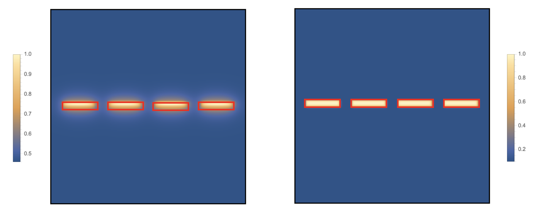
The calculations above assumed an infinite, uniform conductive plane. This can be a good approximation when the inverse momentum transfer is much smaller than geometric features other than the thickness of the film. However, some types of thin film detectors have transverse structure on small scales. For examples, SNSPDs Rosfjord et al. 2006b; Reddy et al. 2020; Verma et al. 2020b use a wire meander with small width (10s to 100s of nm), as illustrated in Figure 6, so for momentum transfers , we might expect this structure to have some effects on scattering rates.
To estimate these effects, we can solve for the 2D electrostatic response across the wire’s cross-section (the meander length is generally long enough that end effects are unimportant). Similarly to the 1D case, we want to solve the Poisson equation, , with . Since doing this analytically is somewhat difficult for general geometries, we can instead discretise it on a 2D grid, and solve the resulting system of equations numerically to obtain .
The simplest way to do this is to impose periodic boundary conditions, which means that we are effectively solving for the response of a series of equally-spaced, infinitely-long wires. The corresponding two-dimensional cross-section is shown in the lower panel of Figure 6, and some example numerical solutions for are shown in Figure 7. The latter illustrate that, for , the response is dominantly contained within the conductor, while for , the response extends over a range , and approximates that from a uniform layer. The dashed curves in Figure 5 compare the numerical scattering rates derived from these solutions to the analytic rates for an equivalent uniform film, illustrating that these match well at , while being volumetrically suppressed at larger .


VI Anisotropic velocity distributions
In our calculations so far, we have adopted the approximation of an isotropic DM velocity distribution. However, it is expected that, due to the velocity of the Earth with respect to the Galactic frame, the DM velocity distribution in the laboratory will be significantly anisotropic (c.f. Appendix B).
Since the direction of this anisotropy in the lab frame will vary over each day as the Earth rotates, a detector for which the scattering rate depends on the direction of the incoming DM will see a daily modulation in scattering rate. The conductor-dielectric heterostructures we have been considering do have anisotropic structures, so even in the approximation where the individual materials have isotropic response functions, the overall scattering rate will still depend on the DM direction.
For the truncated Maxwell-Boltzmann distribution described in Appendix B, and considering a thin-film detector with the parameters given in Section V, Figure 8 shows the ratio of the DM scattering rates for the extreme cases of the velocity offset being parallel and perpendicular to the film (other directions give intermediate rates). For a light mediator, the effect on the overall scattering rate is . Roughly speaking, this is because the phase space volume of mostly-parallel momentum transfers (which maximize collective effects) is larger for parallel DM velocities, but sits at smaller for perpendicular DM velocities. Since small- scatterings are enhanced for a light mediator, these effects partially cancel out, reducing the difference between perpendicular and parallel DM velocities. For heavy mediators, the ratio can be .
More complicated geometries, which modify the -dependence of the structure’s response, can also enhance the ratio between scattering rates for different DM directions. For example, in the ‘SNSPD’ geometry considered in Section V.2, the wire width provides an additional scale. Numerical calculations, of the kind illustrated in Figure 7, indicate that this could significantly increase the directional dependence (integrating over the full velocity distribution to obtain the analogue of Figure 8 would be possible, but computationally expensive — we leave detailed investigations to future work).
It should be emphasised that the specific calculations described above assume that the conductor and dielectric materials both have isotropic and -independent . For large enough frequencies and momentum transfers, this will be a poor approximation. In addition, for thin enough layers, edge effects may become important, even for materials with fairly isotropic bulk permittivities, complicating matters still further. As a result, Figure 8 should not be taken as a realistic prediction of daily modulation amplitudes. However, it does illustrate that the geometrical properties of heterostructures can lead to significant directional dependence, even in situations where the bulk material properties would not do so. This could help to distinguish a dark matter signal from laboratory backgrounds.
As well as daily modulation due to the rotation of the Earth, there is also an annual effect caused by the Earth’s changing velocity around the Sun. This leads to the Earth’s velocity relative to the Galactic frame changing by over the course of the year, with the RMS DM speed varying by . For a light mediator, this generally leads to small (percent-level) differences in the scattering rate, with larger () differences for a heavy mediator.
VII Other mediators
As mentioned above, the prescription, and the associated sum rules, apply in the case of a mediator that couples to EM charge. For mediators with different SM couplings, we need to consider the in-medium self-energy of that mediator, rather than the SM photon, as outlined in Appendix A.
In many circumstances, for light DM with a mediator that is not nucleophilic, the material’s response is dominated by the more mobile electrons, and the formulae give approximately the right results. This is true for most excitations at frequencies . However, for excitations in which nuclei play a significant part, such as phonons, this will no longer be the case. In particular, scattering into such excitations can violate the sum rule bounds, and allow larger rates than those for a dark photon mediator.
As an example, we can consider DM scattering via a scalar mediator which couples to electrons, but not to nucleons. For momentum transfers small enough compared to the material’s inverse lattice scale, the mediator’s effect will correspond to a coherent forcing, and we can excite acoustic phonons, rather than just optical phonons. If the material’s sound speed is large enough, then the enhancement due to the coherent coupling to acoustic phonons can be greater than the suppression due to the velocity mismatch between acoustic phonons and typical DM velocities. Consequently, acoustic phonons can dominate the scattering rate.
This case was analysed in Griffin et al. 2018b; Trickle et al. 2020; in particular, Trickle et al. 2020 performed a density functional theory calculation for the scattering rate in GaAs, plotted in Figure 9. While this calculation did not take into account screening, the scattering rate was dominated by acoustic phonons at small DM masses, for which screening should not be an important effect. As Figure 9 shows, the scattering rate is orders of magnitude below the sum rule limit for a mediator coupling to charge, illustrating how these limits do not apply for other types of coupling. To obtain other examples, we can translate the scattering rates for a nucleophilic scalar mediator calculated in Griffin et al. 2020; at small enough momentum transfers, the coupling of a leptophilic mediator to acoustic phonons can be related to that of a nucleophilic mediator by comparing the nucleon density to the electron density. Figure 9 shows this translation for the diamond calculation from Griffin et al. 2020, illustrating how diamond’s faster sound speed results in larger scattering rates for small DM masses.
Even for a scalar mediator with equal and opposite couplings to electrons and protons, the different velocities of electrons and protons in materials will mean that it has some non-zero coupling to neutral bulk matter. Consequently, it can couple coherently to acoustic phonons. Given that un-suppressed couplings to acoustic phonons can result in very large scattering rates (c.f. Figure 9), we might wonder whether corrections suppressed by the SM fermion velocities could dominate the scattering rate at low DM masses, even for a scalar mediator coupling to charge. To estimate this, we can note that for a non-relativistic fermion. Typical inner-shell electron velocites are , while proton velocities in nuclei are . As a result, we expect typical deviations from bulk neutrality at the level, with the consequence that scattering into acoustic phonons may well be important for low-mass DM. Of course, it is difficult for DM models with a non-nucleophilic scalar mediator to account for all of dark matter without running into other constraints Knapen et al. 2017, and for a small enough dark matter sub-component, even the scattering rates possible with a leptophilic mediator are somewhat hard to probe experimentally Trickle et al. 2020, given existing bounds. Consequently, models where the scattering rate is further suppressed, such as a scalar mediator coupling to charge, would be even harder to see.
VIII Discussion
In this paper, we have discussed two main topics; how electromagnetic sum rules place bounds on the DM-electron scattering rate in materials, and how conductor-dielectric heterostructures can increase the scattering rate of low-mass DM, relative to bulk conductors.
To detect DM, there must be a high enough DM-target scattering rate, and we must be able to detect scatterings that occur. In most of this paper, we have focussed on the first requirement, but the second is also crucial. The very simplest way to ensure detection is for scatterings to deposit energy in the detector material itself. We have pointed out that, for thin-film superconducting detectors, which are one of the most promising routes towards low energy thresholds, geometric effects analogous to those for periodic metal-dielectric heterostructures can have a significant impact on the scattering rate for low-mass DM.
To achieve sensitivity to smaller DM couplings, volume-filling targets will be required, and further work would be needed to establish whether heterostructures could be practically useful. In particular, whether suitable materials could be manufactured, and whether excitations deposited in such materials could be reliably detected, are not obvious.
As mentioned in footnote 7, an interesting question is whether materials with large and negative (inverse) static dielectric function , which have larger frequency-integrated energy loss functions, could be useful for DM detection. The most obvious examples of such systems, such as materials near the threshold of crystallisation, are high-temperature systems that are not suitable for detecting small energy depositions. We leave the investigation of possible alternatives to future work.
Beyond applications to DM detection experiments in the laboratory, our sum rule analyses may also point to other areas in which DM-SM scattering rate calculations need revision. For example, many papers have attempted to calculate the scattering rate for DM passing through the dense interiors of neutron stars or white dwarfs (see Bell et al. 2020; Bell et al. 2021a; Bell et al. 2021b and references therein). However, while such calculations included Pauli blocking, they did not include in-medium effects such as screening. For appropriate mediators, and sufficiently light DM, these may significantly affect the scattering rate. As an example, if we consider a heavy dark photon mediator, then the appropriate sum rule limit for the DM scattering rate is significantly lower than both the electron and nucleon scattering rates given in Bell et al. 2021b for a white dwarf core, for dark matter masses . These topics are explored in DeRocco et al. 2022.
Acknowledgements.
We thank Karl Berggren, Yonit Hochberg, Simon Knapen, Tongyan Lin, Tanner Trickle, and Zhengkang Zhang for helpful conversations, and Yonit Hochberg, Simon Knapen, Tongyan Lin and Zhengkang Zhang for comments on drafts. RL’s research is supported in part by the National Science Foundation under Grant No. PHYS-2014215, and the Gordon and Betty Moore Foundation Grant GBMF7946. RL thanks the Caltech physics department for hospitality during the completion of this work. AP’s research is supported by National Science Foundation under Grant No. PHYS-1720397 and the Gordon and Betty Moore Foundation Grant GBMF7946. AP acknowledges the support of the Fletcher Jones Foundation and the National Science Foundation (NSF) Graduate Research Fellowship Program.Appendix A DM scattering rate formulae
In this appendix, we will give a condensed derivation of the DM scattering rate formula in Eq. (2), explaining the approximations being made.
A.1 Vector mediator
For concreteness, we will start by considering the case of a DM fermion , interacting with a vector mediator , with coupling .
To evaluate the interaction rate of a DM fermion travelling through a medium, we can compute the fermion’s in-medium self-energy. At leading order in , this is given by the imaginary part of the following diagram
where the dashed circle represents the SM medium effects. In the notation of Bellac 2011, the cut self-energy is
| (21) |
where is the cut propagator for (in vacuum, since we assume that is weakly coupled and its density is low), and is the in-medium cut propagator for the mediator. Using the expression for a Dirac fermion, this is.
| (22) |
Writing , the fermion’s interaction rate is given by Bellac 2011
| (23) |
Evaluating the Dirac trace, we have
| (24) |
Assuming that the mediator couples weakly to the SM medium, the dominant contribution to comes from having only SM states in the shaded circle. In this case, we have (to leading order in the SM-mediator coupling) Bellac 2011
| (25) | ||||
where , is the free cut propagator, is the bosonic thermal occupation number for the temperature of the medium, and is the mediator’s in-medium self-energy. The real part of does not contribute, since the integral for only receives contributions from , where the mediator is always off-shell. Going forwards, we will assume that the temperature of our medium is negligible, so we can neglect the term.
Using the fact that (which holds if the current we couple to is conserved), we can write
| (26) |
where is such that is on-shell. Here, since we are assuming negligible medium temperature, we integrate over such that (as upscattering cannot occur).
So far, our calculation has been fully relativistic. If the incoming DM is non-relativistic in the rest frame of the medium, so , then the only part of the term in Eq. (26) that is not suppressed for is the 00 component, which is . This picks out the longitudinal part of , since (note that our convention differs from that of Bellac 2011, which takes ). As we will show below (in Section A.1.1), considering only the term gives the leading contribution for , with
| (27) |
since .
Specialising to a dark photon mediator with kinetic mixing , we have
| (28) |
where is the in-medium propagator for the SM photon, in Lorenz gauge (for more details, see Appendix D of DeRocco et al. 2022). The longitudinal dielectric function is related to the longitudinal part (defined via , where is the longitudinal projector) as Altherr and Kraemmer 1992, so we can write the DM scattering rate as
| (29) |
where puts the DM particle on-shell, in agreement with Eq. (2).
A.1.1 Sub-leading contributions
In the expression, terms other than the 00 component are suppressed by powers of . However, if could be much larger for these other components, then they could still be important. For example, we might worry that, since the exchange of a transverse photon is unscreened for small , whereas longitudinal exchange is screened Bellac 2011, transverse contributions might become important. However, for the case of a dark photon mediator, obeys additional sum rules which mean that the velocity-averaged scattering rate is dominated by the longitudinal-exchange expression in Eq. (27) above, as we show here.
If is a charge density perturbation with wavevector , then the medium’s EM field response is given by , where is the retarded in-medium propagator for the photon. Consequently, writing , the time-averaged power extracted from the charge perturbation is set by . If the medium is in its ground state, then this power should be positive for any perturbing current — that is, the medium should absorb energy from the perturbation, rather than emitting energy. Current conservation implies that , so for any vector perpendicular to , we should have that .
At high enough frequencies, corresponding to timescales much faster than the response times of the system’s matter, the response function should be almost equal to that in vacuum. If we fix the spatial vector , then for the spatial directions transverse to , the response function at large will be . Consequently, the Kramers-Kronig relations give
| (30) |
This equation is not immediately useful as a sum rule, since the integrand may not always be non-negative. However, if we take (without loss of generality), then and correspond to for a spatial vector which is perpendicular to for all , so are always positive. Consequently, we have
| (31) |
where the integrand is always positive, and similarly for , giving us sum rules for the transverse components of the propagator.
If we are interested in the -averaged scattering rate, for an isotropic distribution, then the appropriate integrand arising from Eq. (26) is
| (32) |
where the angle brackets denote averaging over . The contributions from the terms can be bounded using the sum rule from Eq. (31). The terms can be related to , so can be bounded using the sum rule from Eq. (4). Doing so, we find that all of the other terms have -suppressed contributions compared to , which gives rise to Eq. (29).
If we are interested in the -averaged scattering rate, for an isotropic distribution, then the appropriate integrand arising from Eq. (26) is
| (33) |
where the angle brackets denote averaging over (the use of the retarded propagator does not make a difference here). The contributions from the terms can be bounded using the sum rule from Eq. (31). The terms can be related to , so can be bounded using the sum rule from Eq. (4). Doing so, we find that all of the other terms have -suppressed contributions compared to , which gives rise to Eq. (29).
A.2 Scalar mediator
For a scalar mediator , we have
| (34) | ||||
| (35) |
and
| (36) | ||||
where is the mediator’s in-medium self-energy. Evaluating the Dirac trace for the scattering rate,
| (37) |
For a non-relativistic , this is the same, to leading order, as the leading component of the vector mediator’s trace, so we have
| (38) |
If couples with opposite strength to electrons and protons, then to leading order in the velocities of the electrons and protons, is the same as the expression for a vector mediator.
We would obtain similar expressions if we considered scalar DM. Compared to the non-relativistic calculations in Hochberg et al. 2021a; Knapen et al. 2021a, which were spin-agnostic by construction, our calculations illustrate how to incorporate relativistic corrections, as well as mediators with different couplings.
Appendix B DM velocity distribution
The DM scattering rate in an experiment will depend on the DM velocity distribution at Earth. While we do not have precise measurements of this distribution, a common model assumed in the direct detection literature is the truncated Maxwell-Boltzmann distribution McCabe 2010; Lisanti 2016. Writing as the velocity relative to Earth, the DM velocity distribution is taken to be
| (39) |
where
| (40) |
Standard values taken for these parameters are , , Griffin et al. 2020.
In the limit (corresponding to a simple Maxwell-Boltzmann distribution in the Galactic frame, which can be useful for seeing the basic form of expressions), we have . From Section II.2, a useful quantity for computing DM scattering rates is
| (41) |
For a Maxwell-Boltzmann distribution, this is
| (42) |
For the truncated Maxwell-Boltzmann distribution, we have
| (43) |
Figure 10 plots for the standard parameter values, illustrating that the difference between the truncated and non-truncated Maxwell-Boltzmann distributions is only important at high velocities, and correspondingly small values.
Appendix C Other EM sum rules
As well as the sum rule, there are also other constraints that the longitudinal dielectric function should satisfy Mahan 2000; Dressel and Grüner 2002. For example, suppose that for large enough . Then, from the Kramers-Kronig relations,
| (44) |
The sum rule (Eq. (1)) can be viewed as corresponding to energy absorption from a delta-function pulse in time. In contrast, the sum rule from Eq. (44) corresponds to energy absorption from a second-derivative-of-delta-function pulse (a rapid down-up-down sequence). This emphasises absorption at higher frequencies. Physically, since we are interested in low-mass DM absorption, and correspondingly, in smaller energy transfers, the sum rule will be more useful for our purposes.
References
- Schumann (2019) M. Schumann, J. Phys. G 46, 103003 (2019), arXiv:1903.03026 [astro-ph.CO] .
- Lee and Weinberg (1977) B. W. Lee and S. Weinberg, Physical Review Letters 39, 165 (1977).
- Bœhm and Fayet (2004) C. Bœhm and P. Fayet, Nuclear Physics B 683, 219 (2004).
- Chang et al. (2021) J. H. Chang, R. Essig, and A. Reinert, Journal of High Energy Physics 2021 (2021), 10.1007/jhep03(2021)141.
- Dvorkin et al. (2019) C. Dvorkin, T. Lin, and K. Schutz, Physical Review D 99 (2019), 10.1103/physrevd.99.115009.
- Hall et al. (2010) L. J. Hall, K. Jedamzik, J. March-Russell, and S. M. West, Journal of High Energy Physics 2010 (2010), 10.1007/jhep03(2010)080.
- Essig et al. (2012a) R. Essig, J. Mardon, and T. Volansky, Phys. Rev. D 85, 076007 (2012a), arXiv:1108.5383 [hep-ph] .
- Essig et al. (2012b) R. Essig, A. Manalaysay, J. Mardon, P. Sorensen, and T. Volansky, Phys. Rev. Lett. 109, 021301 (2012b), arXiv:1206.2644 [astro-ph.CO] .
- Essig et al. (2016) R. Essig, M. Fernandez-Serra, J. Mardon, A. Soto, T. Volansky, and T.-T. Yu, JHEP 05, 046 (2016), arXiv:1509.01598 [hep-ph] .
- Hochberg et al. (2016a) Y. Hochberg, Y. Zhao, and K. M. Zurek, Phys. Rev. Lett. 116, 011301 (2016a), arXiv:1504.07237 [hep-ph] .
- Hochberg et al. (2016b) Y. Hochberg, M. Pyle, Y. Zhao, and K. M. Zurek, JHEP 08, 057 (2016b), arXiv:1512.04533 [hep-ph] .
- Hochberg et al. (2017) Y. Hochberg, Y. Kahn, M. Lisanti, C. G. Tully, and K. M. Zurek, Phys. Lett. B 772, 239 (2017), arXiv:1606.08849 [hep-ph] .
- Hochberg et al. (2018) Y. Hochberg, Y. Kahn, M. Lisanti, K. M. Zurek, A. G. Grushin, R. Ilan, S. M. Griffin, Z.-F. Liu, S. F. Weber, and J. B. Neaton, Phys. Rev. D 97, 015004 (2018), arXiv:1708.08929 [hep-ph] .
- Derenzo et al. (2017) S. Derenzo, R. Essig, A. Massari, A. Soto, and T.-T. Yu, Phys. Rev. D 96, 016026 (2017), arXiv:1607.01009 [hep-ph] .
- Kurinsky et al. (2019) N. A. Kurinsky, T. C. Yu, Y. Hochberg, and B. Cabrera, Phys. Rev. D 99, 123005 (2019), arXiv:1901.07569 [hep-ex] .
- Griffin et al. (2020) S. M. Griffin, K. Inzani, T. Trickle, Z. Zhang, and K. M. Zurek, Phys. Rev. D 101, 055004 (2020).
- Blanco et al. (2020) C. Blanco, J. I. Collar, Y. Kahn, and B. Lillard, Phys. Rev. D 101, 056001 (2020), arXiv:1912.02822 [hep-ph] .
- Trickle et al. (2020) T. Trickle, Z. Zhang, K. M. Zurek, K. Inzani, and S. Griffin, JHEP 03, 036 (2020), arXiv:1910.08092 [hep-ph] .
- Geilhufe et al. (2020) R. M. Geilhufe, F. Kahlhoefer, and M. W. Winkler, Physical Review D 101 (2020), 10.1103/physrevd.101.055005.
- Hochberg et al. (2019) Y. Hochberg, I. Charaev, S.-W. Nam, V. Verma, M. Colangelo, and K. K. Berggren, Phys. Rev. Lett. 123, 151802 (2019), arXiv:1903.05101 [hep-ph] .
- Coskuner et al. (2021a) A. Coskuner, A. Mitridate, A. Olivares, and K. M. Zurek, Physical Review D 103 (2021a), 10.1103/physrevd.103.016006.
- Griffin et al. (2021) S. M. Griffin, Y. Hochberg, K. Inzani, N. Kurinsky, T. Lin, and T. C. Yu, Phys. Rev. D 103, 075002 (2021), arXiv:2008.08560 [hep-ph] .
- Knapen et al. (2017) S. Knapen, T. Lin, and K. M. Zurek, Phys. Rev. D 96, 115021 (2017), arXiv:1709.07882 [hep-ph] .
- Hochberg et al. (2021a) Y. Hochberg, Y. Kahn, N. Kurinsky, B. V. Lehmann, T. C. Yu, and K. K. Berggren, Phys. Rev. Lett. 127, 151802 (2021a), arXiv:2101.08263 [hep-ph] .
- Knapen et al. (2021a) S. Knapen, J. Kozaczuk, and T. Lin, Physical Review D 104 (2021a), 10.1103/physrevd.104.015031.
- Nozières and Pines (1959) P. Nozières and D. Pines, Phys. Rev. 113, 1254 (1959).
- Mahan (2000) G. D. Mahan, Many-Particle Physics (Springer, Boston, MA, 2000).
- Dressel and Grüner (2002) M. Dressel and G. Grüner, Electrodynamics of Solids (Cambridge University Press, 2002).
- Dreyling-Eschweiler (2014) J. Dreyling-Eschweiler (ALPS-II), in Proceedings, 10th Patras Workshop on Axions, WIMPs and WISPs (AXION-WIMP 2014): Geneva, Switzerland, June 29-July 4, 2014 (2014) pp. 63–66, arXiv:1409.6992 [physics.ins-det] .
- Dreyling-Eschweiler et al. (2015) J. Dreyling-Eschweiler, N. Bastidon, B. Döbrich, D. Horns, F. Januschek, and A. Lindner, J. Mod. Opt. 62, 1132 (2015), arXiv:1502.07878 [physics.ins-det] .
- Cabrera et al. (1998) B. Cabrera, R. M. Clarke, P. Colling, A. J. Miller, S. Nam, and R. W. Romani, Applied Physics Letters 73, 735 (1998), https://doi.org/10.1063/1.121984 .
- Karasik et al. (2012) B. S. Karasik, S. V. Pereverzev, A. Soibel, D. F. Santavicca, D. E. Prober, D. Olaya, and M. E. Gershenson, Appl. Phys. Lett. 101, 052601 (2012), arXiv:1207.2164 [physics.ins-det] .
- Lita et al. (2008) A. E. Lita, A. J. Miller, and S. W. Nam, Opt. Express 16, 3032 (2008).
- Bastidon et al. (2015) N. Bastidon, D. Horns, and A. Lindner (2015) arXiv:1509.02064 [physics.ins-det] .
- Mazin (2009) B. A. Mazin, in American Institute of Physics Conference Series, American Institute of Physics Conference Series, Vol. 1185, edited by B. Young, B. Cabrera, and A. Miller (2009) pp. 135–142.
- Day et al. (2003) P. Day, H. Leduc, B. A Mazin, A. Vayonakis, and J. Zmuidzinas, Nature, 425, 817 (2003).
- Gao et al. (2012) J. Gao, M. R. Vissers, M. O. Sandberg, F. C. S. da Silva, S. W. Nam, D. P. Pappas, D. S. Wisbey, E. C. Langman, S. R. Meeker, B. A. Mazin, H. G. Leduc, J. Zmuidzinas, and K. D. Irwin, Applied Physics Letters 101, 142602 (2012), https://doi.org/10.1063/1.4756916 .
- Rosfjord et al. (2006a) K. M. Rosfjord, J. K. W. Yang, E. A. Dauler, A. J. Kerman, V. Anant, B. M. Voronov, G. N. Gol’tsman, and K. K. Berggren, Opt. Express 14, 527 (2006a).
- Reddy et al. (2020) D. V. Reddy, R. R. Nerem, S. W. Nam, R. P. Mirin, and V. B. Verma, Optica 7, 1649 (2020).
- Verma et al. (2020a) V. B. Verma et al., “Single-photon detection in the mid-infrared up to 10 micron wavelength using tungsten silicide superconducting nanowire detectors,” (2020a), arXiv:2012.09979 [physics.ins-det] .
- Wollman et al. (2017) E. E. Wollman et al., Opt. Express 25, 26792 (2017).
- Hochberg et al. (2021b) Y. Hochberg, B. Lehmann, I. Charaev, J. Chiles, S.-W. Nam, and K. K. Berggren, (2021b), arXiv:2110.01586 [hep-ph] .
- Bunting et al. (2017) P. C. Bunting, G. Gratta, T. Melia, and S. Rajendran, Phys. Rev. D 95, 095001 (2017), arXiv:1701.06566 [hep-ph] .
- Dolgov et al. (1981) O. V. Dolgov, D. A. Kirzhnits, and E. G. Maksimov, Reviews of Modern Physics 53, 81 (1981).
- DeRocco et al. (2022) W. DeRocco, M. Galanis, and R. Lasenby, (2022), arXiv:2201.05167 [hep-ph] .
- Carney et al. (2021) D. Carney, H. Häffner, D. C. Moore, and J. M. Taylor, (2021), arXiv:2104.05737 [quant-ph] .
- Budker et al. (2021) D. Budker, P. W. Graham, H. Ramani, F. Schmidt-Kaler, C. Smorra, and S. Ulmer, (2021), arXiv:2108.05283 [hep-ph] .
- Sun et al. (2016) Y. Sun, H. Xu, B. Da, S.-f. Mao, and Z.-j. Ding, Chinese Journal of Chemical Physics 29, 663 (2016), https://doi.org/10.1063/1674-0068/29/cjcp1605110 .
- Knapen et al. (2021b) S. Knapen, J. Kozaczuk, and T. Lin, (2021b), arXiv:2104.12786 [hep-ph] .
- Coskuner et al. (2021b) A. Coskuner, T. Trickle, Z. Zhang, and K. M. Zurek, (2021b), arXiv:2102.09567 [hep-ph] .
- Knapen et al. (2018a) S. Knapen, T. Lin, M. Pyle, and K. M. Zurek, Phys. Lett. B 785, 386 (2018a), arXiv:1712.06598 [hep-ph] .
- Griffin et al. (2018a) S. Griffin, S. Knapen, T. Lin, and K. M. Zurek, Phys. Rev. D 98, 115034 (2018a), arXiv:1807.10291 [hep-ph] .
- (53) T. Trickle and Z. Zhang, personal communication.
- Gelmini et al. (2020) G. B. Gelmini, V. Takhistov, and E. Vitagliano, Phys. Lett. B 809, 135779 (2020), arXiv:2006.13909 [hep-ph] .
- Fasolino et al. (1978) A. Fasolino, M. Parrinello, and M. Tosi, Physics Letters A 66, 119 (1978).
- Geilhufe et al. (2018) R. M. Geilhufe, B. Olsthoorn, A. D. Ferella, T. Koski, F. Kahlhoefer, J. Conrad, and A. V. Balatsky, physica status solidi (RRL) - Rapid Research Letters 12, 1800293 (2018).
- Knickerbocker and Kulkarni (1996) S. A. Knickerbocker and A. K. Kulkarni, Journal of Vacuum Science & Technology A: Vacuum, Surfaces, and Films 14, 757 (1996).
- Bozovic (1990) I. Bozovic, Physical Review B 42, 1969 (1990).
- Kuz’michev and Motulevich (1983) N. D. Kuz’michev and G. P. Motulevich, “Determination of the electron characteristics of niobium nitride by an optical method,” (1983).
- Cai and Shalaev (2010) W. Cai and V. Shalaev, Optical Metamaterials (Springer New York, 2010).
- Maleeva et al. (2018) N. Maleeva, L. Grünhaupt, T. Klein, F. Levy-Bertrand, O. Dupre, M. Calvo, F. Valenti, P. Winkel, F. Friedrich, W. Wernsdorfer, A. V. Ustinov, H. Rotzinger, A. Monfardini, M. V. Fistul, and I. M. Pop, Nature Communications 9 (2018), 10.1038/s41467-018-06386-9.
- Vogel and Redondo (2014) H. Vogel and J. Redondo, Journal of Cosmology and Astroparticle Physics 2014, 029 (2014).
- Chang et al. (2018) J. H. Chang, R. Essig, and S. D. McDermott, Journal of High Energy Physics 2018 (2018), 10.1007/jhep09(2018)051.
- Essig et al. (2012c) R. Essig, A. Manalaysay, J. Mardon, P. Sorensen, and T. Volansky, Physical Review Letters 109 (2012c), 10.1103/physrevlett.109.021301.
- Essig et al. (2017) R. Essig, T. Volansky, and T.-T. Yu, Physical Review D 96 (2017), 10.1103/physrevd.96.043017.
- Yakubovsky et al. (2017) D. I. Yakubovsky, A. V. Arsenin, Y. V. Stebunov, D. Y. Fedyanin, and V. S. Volkov, Optics Express 25, 25574 (2017).
- Chiles et al. (2021) J. Chiles, I. Charaev, R. Lasenby, M. Baryakhtar, J. Huang, A. Roshko, G. Burton, M. Colangelo, K. Van Tilburg, A. Arvanitaki, S.-W. Nam, and K. K. Berggren, (2021), arXiv:2110.01582 [hep-ex] .
- Polakovic et al. (2020) T. Polakovic, W. Armstrong, G. Karapetrov, Z.-E. Meziani, and V. Novosad, Nanomaterials 10, 1198 (2020).
- Knapen et al. (2018b) S. Knapen, T. Lin, M. Pyle, and K. M. Zurek, Physics Letters B 785, 386–390 (2018b).
- Griffin et al. (2018b) S. Griffin, S. Knapen, T. Lin, and K. M. Zurek, Phys. Rev. D 98, 115034 (2018b).
- Rosfjord et al. (2006b) K. M. Rosfjord, J. K. W. Yang, E. A. Dauler, A. J. Kerman, V. Anant, B. M. Voronov, G. N. Gol’tsman, and K. K. Berggren, Opt. Express 14, 527 (2006b).
- Verma et al. (2020b) V. B. Verma, B. Korzh, A. B. Walter, A. E. Lita, R. M. Briggs, M. Colangelo, Y. Zhai, E. E. Wollman, A. D. Beyer, J. P. Allmaras, B. Bumble, H. Vora, D. Zhu, E. Schmidt, K. K. Berggren, R. P. Mirin, S. W. Nam, and M. D. Shaw, “Single-photon detection in the mid-infrared up to 10 micron wavelength using tungsten silicide superconducting nanowire detectors,” (2020b), arXiv:2012.09979 [physics.ins-det] .
- Bell et al. (2020) N. F. Bell, G. Busoni, S. Robles, and M. Virgato, JCAP 09, 028 (2020), arXiv:2004.14888 [hep-ph] .
- Bell et al. (2021a) N. F. Bell, G. Busoni, S. Robles, and M. Virgato, JCAP 03, 086 (2021a), arXiv:2010.13257 [hep-ph] .
- Bell et al. (2021b) N. F. Bell, G. Busoni, M. E. Ramirez-Quezada, S. Robles, and M. Virgato, (2021b), arXiv:2104.14367 [hep-ph] .
- Bellac (2011) M. L. Bellac, Thermal Field Theory (Cambridge University Press, 2011).
- Altherr and Kraemmer (1992) T. Altherr and U. Kraemmer, Astroparticle Physics 1, 133 (1992).
- McCabe (2010) C. McCabe, Physical Review D 82 (2010), 10.1103/physrevd.82.023530.
- Lisanti (2016) M. Lisanti, in New Frontiers in Fields and Strings (WORLD SCIENTIFIC, 2016).