COFFEE: COVID-19 Forecasts using Fast Evaluations and EstimationApproved for unlimited release and assigned number LA-UR-20-28630

Lauren Castro Affiliation: Information Systems and Modeling Group, Los Alamos National Laboratory Affiliation: Center for Nonlinear Studies, Los Alamos National Laboratory Geoffrey Fairchild Affiliation: Information Systems and Modeling Group, Los Alamos National Laboratory Isaac Michaud Affiliation: Statistical Sciences Group, Los Alamos National Laboratory Dave Osthus Affiliation: Statistical Sciences Group, Los Alamos National Laboratory

Abstract

This document details the methodology of the Los Alamos National Laboratory COVID-19 forecasting model, COFFEE (COVID-19 Forecasts using Fast Evaluations and Estimation).

COFFEE Methodology

COFFEE is a probabilistic model that forecasts daily reported cases and deaths of COVID-19. COFFEE is fit to geographic regions independently, facilitating parallelization for fast computations.

Notation

•

$t$ indexes time, where $t$ is the number of days from a reference starting date (index)
•

$T$ is the day of the last observation (index)
•

$K$ is the forecast window size, in days (index)
•

$y_{c,t}$ is the number of reported cases of COVID-19 on day $t$ as reported on the COVID-19 Dashboard by the Centers for Systems Science Engineering (CSSE) at Johns Hopkins University (JHU) (observable)
•

$\ddot{y}_{c,t}=\sum_{j=1}^{t}y_{c,j}$ is the cumulative number of reported cases of COVID-19 through day $t$ as reported by CSSE at JHU (observable)
•

$y_{d,t}$ is the number of reported deaths of COVID-19 on day $t$ as reported by CSSE at JHU (observable)
•

$\ddot{y}_{d,t}=\sum_{j=1}^{t}y_{d,j}$ is the cumulative number of reported deaths of COVID-19 through day $t$ as reported by CSSE at JHU (observable)
•

$\delta_{c,t}$ is the underlying number of reported cases on day $t$ (unobservable)
•

$\ddot{\delta}_{c,t}=\sum_{j=1}^{t}\delta_{c,j}$ is the underlying number of cumulative reported cases through day $t$ (unobservable)
•

$\delta_{d,t}$ is the underlying number of reported deaths on day $t$ (unobservable)
•

$\ddot{\delta}_{d,t}=\sum_{j=1}^{t}\delta_{d,j}$ is the underlying number of cumulative reported deaths through day $t$ (unobservable)
•

$\delta_{s,0}$ is the underlying number of susceptible individuals at the start of the pandemic (unobservable)
•

$\delta_{s,t}=\delta_{s,0}-\ddot{\delta}_{c,t}$ is the underlying number of susceptible individuals on day $t$ (unobservable)

We use the convention that bolded quantities are vectors and unbolded quantities are scalars. For concreteness, $y_{c,t}$ is a scalar while $\bm{y}_{c,1:t}=(y_{c,1},y_{c,2},\ldots,y_{c,t})^{\prime}$ is a $t\times 1$ vector.

Cases Model

Let

\displaystyle y_{c,t}|\delta_{c,t},\alpha

\displaystyle\sim\text{NB}\Bigg(\delta_{c,t},\frac{\delta_{c,t}}{\alpha}\Bigg)

(1)

where NB(a,b) is a Negative-Binomial model with mean parameter a $>0$ and size parameter b $>0$ where

	$\displaystyle\text{E}(y_{c,t}\|\delta_{c,t},\alpha)$	$\displaystyle=\delta_{c,t}$		(2)
	$\displaystyle\text{Var}(y_{c,t}\|\delta_{c,t},\alpha)$	$\displaystyle=\delta_{c,t}(1+\alpha).$		(3)

Figure 1 shows the daily reported cases for New Mexico, the United States (US), and France. All three regions have gone through rising and declining periods of cases with various levels of noise in the reported cases.

Refer to caption — Figure 1: The daily reported cases of COVID-19 for New Mexico, the US, and France.

In what follows, we outline the steps COFFEE takes to produce forecasts of reported cases.

Step 1: Identify and Adjust Outliers

COFFEE automatically identifies and adjusts outliers [2]. It runs five different outlier detection algorithms on the reported data, taking into account possible day-of-week (DOW) effects. A datum is declared an outlier if three or more of the five detection algorithms identify that datum as an outlier. The outliers are not removed, but rather adjusted to ensure all values are non-negative. Figure 2 shows the result of this process on daily cases for New Mexico, the US, and France. All subsequent modeling steps are conducted with outlier adjusted data.

Step 2: Compute the Empirical Growth Rate, $\hat{\kappa}_{t}$

The model for the underlying number of reported daily cases, $\delta_{c,t}$ , is a dynamic susceptible-infectious (SI) model [1], where

	$\displaystyle\delta_{s,t}$	$\displaystyle=\delta_{s,t-1}-\delta_{c,t}$		(4)
	$\displaystyle\ddot{\delta}_{c,t}$	$\displaystyle=\ddot{\delta}_{c,t-1}+\delta_{c,t},$		(5)

and

\displaystyle\delta_{c,t}=\kappa_{t}\frac{\delta_{s,t-1}}{\delta_{s,0}}\ddot{\delta}_{c,t-1}.

(6)

The quantity $\ddot{\delta}_{c,t-1}$ is the cumulative number of underlying cases on day $t-1$ , $\frac{\delta_{s,t-1}}{\delta_{s,0}}$ is the proportion of the population still susceptible at time $t-1$ , and $\kappa_{t}$ is the growth rate on day $t$ .

When $\frac{\delta_{s,t-1}}{\delta_{s,0}}\approx 1$ (when most of the susceptible population is still susceptible), we can rearrange Equations 4, 5, and 6 to identify a crude estimator of $\kappa_{t}$ :

\displaystyle\hat{\kappa}_{t}

\displaystyle\approx\Bigg(\frac{\ddot{y}_{c,t}}{\ddot{y}_{c,t-1}}-1\Bigg).

(7)

Estimates for $\kappa_{t}$ are shown in Figure 3. It is clear that $\hat{\kappa}_{t}$ is dynamic and changes over time. This is what makes forecasting COVID-19 so challenging; parameters of epidemiologically-motivated models are dynamic and forecasting with them requires anticipating how these dynamic parameters will change in the future, not just tracking where they have been in the past. In what follows, we describe how we forecast $\hat{\kappa}_{t}$ .

Step 3: Compute $\hat{\kappa}^{*}_{t}$ = logit $(\hat{\kappa}_{t})$

After the initial portion of the outbreak, $\hat{\kappa}_{t}$ is almost always between 0 and 1. COFFEE logit transforms $\hat{\kappa}_{t}$ , where logit( $p$ ) = log( $p/(1-p)$ ) for $p\in(0,1)$ . For all days with no reported cases, $\hat{\kappa}_{t}=0$ , an incompatible value with the logit transform. Thus, we compute $\hat{\kappa}^{*}_{t}=$ logit( $\hat{\kappa}_{t}$ ) as follows:

\displaystyle\hat{\kappa}^{*}_{t}

\displaystyle=\begin{cases}\text{logit}(\hat{\kappa}_{t})&\text{ if }\hat{\kappa}_{t}>\tau_{c}\text{ and }\hat{\kappa}_{t}<1-\tau_{c}\\ \text{logit}(\tau_{c})&\text{ if }\hat{\kappa}_{t}\leq\tau_{c}\\ \text{logit}(1-\tau_{c})&\text{ if }\hat{\kappa}_{t}\geq 1-\tau_{c},\\ \end{cases}

(8)

where $\tau_{c}=0.95*\text{min}(\{\hat{\kappa}_{t}|\hat{\kappa}_{t}>0\})$ , ensuring that if $\hat{\kappa}_{t}\geq\hat{\kappa}_{t^{\prime}}$ , then $\hat{\kappa}^{*}_{t}\geq\hat{\kappa}^{*}_{t^{\prime}}$ . The logit transformed $\hat{\kappa}_{t}$ are shown in Figure 4.

Step 4: Split Data into Training and Testing Sets

Let $T$ be the last observed day. We only consider the last 42 days of data when fitting a model for $\hat{\kappa}^{*}_{t}$ and split those days into training and testing data [3]. Days $T-41$ through $T-14$ constitute the training data, while $T-13$ through $T$ constitutes the testing data. We will denote the last day of the training data by $T^{\text{train}}=T-14$ . The splits are shown for New Mexico, the US, and France in Figure 5.

Step 5: Compute $\hat{\kappa}_{t}^{\text{trend}}$

We fit a weighted regression to the training data, where we downweight influential points that could have an outsized influence on the regression using the inverse of Cook’s distance. The regression has a linear trend over time and a DOW effect:

\displaystyle\hat{\kappa}^{*}_{t}

\displaystyle=\beta_{0}+\beta_{1}t+\beta_{2}\text{I}(t=\text{Monday})+\beta_{3}\text{I}(t=\text{Tuesday})+\ldots+\beta_{7}\text{I}(t=\text{Saturday}).

(9)

Variable selection is performed, potentially resulting in a subset of the model parameters in Equation 9. We refer to the fits and predictions from this linear model as $\hat{\kappa}_{t}^{\text{trend}}$ where

\displaystyle\hat{\kappa}_{t}^{\text{trend}}=\hat{\beta}_{0}+\hat{\beta}_{1}t+\hat{\beta}_{2}\text{I}(t=\text{Monday})+\hat{\beta}_{3}\text{I}(t=\text{Tuesday})+\ldots+\hat{\beta}_{7}\text{I}(t=\text{Saturday})

(10)

where, if a variable was removed during the variable selection phase, then the corresponding $\hat{\beta}$ is set equal to 0. Figure 6 shows $\hat{\kappa}^{\text{trend}}_{t}$ for the training and testing windows.

Step 6: Compute $\hat{\kappa}_{t}^{\text{constant}}$

There is a $\hat{\kappa}_{t}$ trajectory corresponding to a constant new number of cases day over day. Let

\displaystyle\bar{y}_{c,T^{\text{train}}}

\displaystyle=\frac{1}{7}\sum_{t=T^{\text{train}}-6}^{T^{\text{train}}}y_{c,t}

(11)

be the average number of daily reported cases over the last week of the training window.

Then

\displaystyle\hat{\kappa}_{t}^{\text{constant}}

\displaystyle=\text{logit}\Bigg(\bar{y}_{c,T^{\text{train}}}\Bigg[\Bigg(\frac{\delta_{s,0}-\ddot{y}_{c,t-1}}{\delta_{s,0}}\Bigg)\ddot{y}_{c,t-1}\Bigg]^{-1}\Bigg)

(12)

where we set $\delta_{s,0}=0.55N$ , where $N$ is the population of the forecasted region and 0.55 is a nominal attack rate for COVID-19. Figure 7 shows $\hat{\kappa}_{t}^{\text{constant}}$ for $t=T^{\text{train}}+k$ and $k\in 1,2,\ldots,14$ .

Step 7: Compute a Joint Probability Distribution over Tuning Parameters

The form of the forecasting model for $\hat{\kappa}_{t}^{\text{forecast}}$ is

\displaystyle\hat{\kappa}_{t}^{\text{forecast}}(\eta,\omega,\phi)

\displaystyle=\lambda_{t}(\phi)[w_{t}\text{min}(\eta^{*},\hat{\kappa}_{t}^{\text{trend}})+(1-w_{t})\hat{\kappa}_{t}^{\text{constant+DOW}}]

(13)

for $t=T^{\text{train}}+k$ and $k\in 1,2,\ldots,14$ . The objective is to produce forecasts for $\hat{\kappa}_{t}$ . The way COFFEE does this is be creating a blended combination of $\hat{\kappa}_{t}^{\text{trend}}$ and $\hat{\kappa}_{t}^{\text{constant+DOW}}$ where

	$\displaystyle\hat{\kappa}_{t}^{\text{constant+DOW}}=$	$\displaystyle\hat{\kappa}_{t}^{\text{constant}}+$
		$\displaystyle\hat{\beta}_{2}\text{I}(t=\text{Monday})+\hat{\beta}_{3}\text{I}(t=\text{Tuesday})+\ldots+\hat{\beta}_{7}\text{I}(t=\text{Saturday}),$		(14)

which is $\hat{\kappa}_{t}^{\text{constant}}$ with the DOW effects estimated in Equation 10 added.

There are three tuning parameters in Equation 13, each playing a role in controlling the form of $\hat{\kappa}_{t}^{\text{forecast}}$ .

The first tuning parameter $\eta$ puts a cap on how large $\hat{\kappa}_{t}^{\text{trend}}$ can get. A forecast can blow up if $\hat{\kappa}_{t}^{\text{trend}}$ is growing in an unmitigated fashion. The parameter $\eta$ is a safeguard against this unmitigated growth. We set

\displaystyle\eta^{*}

\displaystyle=\text{median}(\{\hat{\kappa}^{*}_{T^{\text{train}}-6},\hat{\kappa}^{*}_{T^{\text{train}}-5},\ldots,\hat{\kappa}^{*}_{T^{\text{train}}}\})\eta

(15)

for $\eta\in[0,1]$ .

The second tuning parameter is $\omega$ . The basic form of the forecasting model is to transition from a forecast that relies on the current trend $\hat{\kappa}^{\text{trend}}_{t}$ to a forecast that relies on $\hat{\kappa}^{\text{constant+DOW}}_{t}$ . If $\hat{\kappa}_{t}^{\text{trend}}$ is trending up, this transition keeps the forecasts from blowing up. If $\hat{\kappa}_{t}^{\text{trend}}$ is trending down, this transition keeps the forecasts from flat-lining at 0 new cases. The assumption behind this modeling choice is that, as cases are going up, people will take action to curb the growth of the pandemic, either through independent choices of personal responsibility or governmental policies. As cases are going down, however, we assume policies will be relaxed or people will become more comfortable engaging in activities that will increase transmission pathways. The tuning parameter $\omega\geq 1$ determines how quickly the forecast transitions from $\hat{\kappa}_{t}^{\text{trend}}$ to $\hat{\kappa}_{t}^{\text{constant+DOW}}$ . The closer $\omega$ is to 0, the quicker the transition occurs.

\displaystyle w_{T^{\text{train}}+k}

\displaystyle=\begin{cases}1-\Bigg(\frac{k-1}{\omega}\Bigg)^{2}&\text{ if }k\leq\omega+1\\ 0&\text{ otherwise }\end{cases}

(16)

where $k$ is a positive integer. Figure 8 shows weight trajectories $w_{t}$ for various choices of $\omega$ . When $w_{T^{\text{train}}+k}=1$ , all weight is on $\hat{\kappa}_{t}^{\text{trend}}$ ; when $w_{T^{\text{train}}+k}=0$ , all weight is on $\hat{\kappa}_{t}^{\text{constant+DOW}}$ .

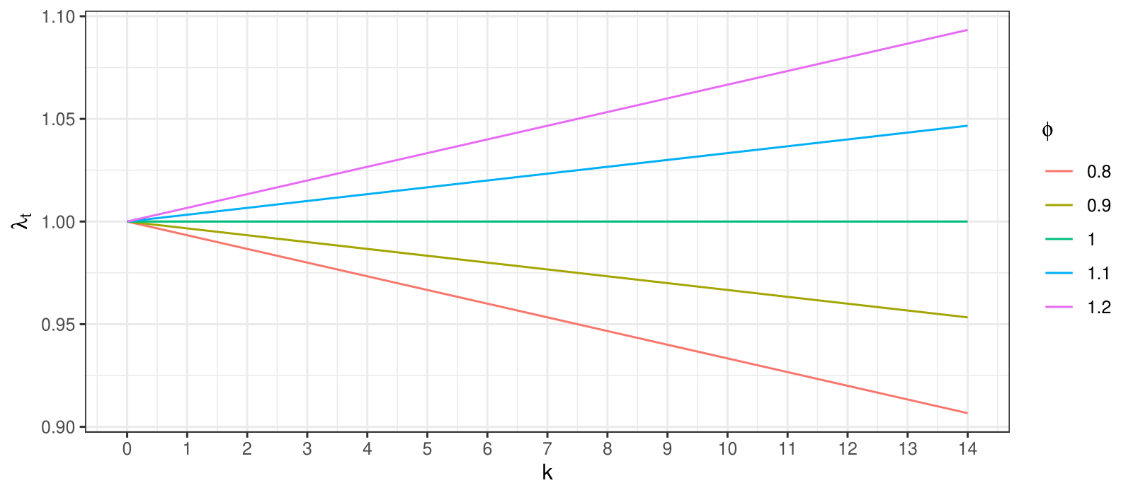
The third tuning parameter is $\phi$ . The trajectory $\lambda_{t}$ is defined as

\displaystyle\lambda_{T^{\text{train}}+k}

\displaystyle=1+k\frac{\phi-1}{30},

(17)

a linear trend starting at 1 when $k=0$ . The tuning parameter $\phi>0$ determines whether $\lambda_{T^{\text{train}}+k}$ trends up ( $\phi>1$ ) or down ( $\phi<1$ ). Examples of $\lambda_{T^{\text{train}}+k}$ are shown in Figure 9.

For a combination of $\eta$ , $\omega$ , and $\phi$ , we compute $\hat{\kappa}_{t}^{\text{forecast}}(\eta,\omega,\phi)$ and compute the inverse-distance between the inverse-logit of $\hat{\kappa}_{t}^{\text{forecast}}(\eta,\omega,\phi)$ and $\hat{\kappa}_{t}$ over the test period:

\displaystyle d^{-1}(\eta,\omega,\phi)

\displaystyle=\Bigg(\sum_{t=T^{\text{train}}+1}^{T^{\text{train}}+14}\Bigg[\text{logit}^{-1}\Bigg(\hat{\kappa}_{t}^{\text{forecast}}(\eta,\omega,\phi)\Bigg)-\hat{\kappa}_{t}\Bigg]^{2}\Bigg)^{-1}.

(18)

Finally we compute a joint probability distribution over $\eta$ , $\omega$ , and $\phi$ as the normalized inverse-distance. The probability distributions for New Mexico, the US, and France are shown in Figure 10.

Step 8: Produce the Reported Cases Forecast

The final step is to simulate reported cases. The purpose of the previous steps was to get a joint probability distribution over the tuning parameters that can be used to sample from.

If more than 14 of the last 28 days had zero reported cases, we take independent and identically distributed (iid) samples of future reported cases from the empirical distribution of outlier adjusted reported cases over the last 28 days. If no cases were reported over the last 28 days, we sample future reported cases as iid Bernoulli draws with success probability equal to 1/29. If 14 or more of the last 28 days observed at least 1 reported case, we simulate $\hat{\kappa}^{\text{forecast}}_{T+k}$ for $k\in{1,2,...,K}$ by doing the following:

1.

Do Step 5, treating the training data as days $T$ to $T-27$ , resulting in a fitted linear model in the form of Equation 9. Use this to compute $\hat{\kappa}^{\text{trend}}_{T+k}$ .
2.

Do Step 6 to compute $\hat{\kappa}^{\text{constant+DOW}}_{T+k}$ , replacing $T^{\text{train}}$ with $T$ in Equations 11 and 12.
3.

Draw a vector of $(\omega,\phi,\eta)$ from the joint distribution computed in Step 7.
4.

Compute $\hat{\kappa}_{T+k}^{\text{forecast}}$ following Equation 13.
5.

Compute logit ${}^{-1}(\hat{\kappa}_{T+k}^{\text{forecast}})$ .
6.

Draw an attack rate $p\sim\text{Uniform}(0.4,0.7)$ and set $\delta^{\text{forecast}}_{s,0}=pN$ .
7.

Set $\ddot{\delta}_{c,T}=\ddot{y}_{c,T}$ and $\delta_{s,T}=\delta^{\text{forecast}}_{s,0}-\ddot{y}_{c,T}$
8.
For $k=1,2,\ldots,K$ , compute
1. (a)
  
  $\delta^{\text{forecast}}_{c,T+k}=\text{logit}^{-1}(\hat{\kappa}_{T+k}^{\text{forecast}})\Bigg(\frac{\delta^{\text{forecast}}_{s,T+k-1}}{\delta^{\text{forecast}}_{s,0}}\Bigg)\ddot{\delta}^{\text{forecast}}_{c,T+k-1}$
2. (b)
  
  $\ddot{\delta}^{\text{forecast}}_{c,T+k}=\ddot{\delta}^{\text{forecast}}_{c,T+k-1}+\delta^{\text{forecast}}_{c,T+k}$
3. (c)
  
  $\delta^{\text{forecast}}_{s,T+k}=\delta^{\text{forecast}}_{s,T+k-1}-\delta^{\text{forecast}}_{c,T+k}$
9.

Draw $y^{\text{forecast}}_{c,t}|\delta^{\text{forecast}}_{c,T+k},\hat{\alpha}\sim\text{NB}\Bigg(\delta^{\text{forecast}}_{c,T+k},\frac{\delta^{\text{forecast}}_{c,T+k}}{\hat{\alpha}}\Bigg)$ where $\hat{\alpha}$ is the maximum likelihood estimate.

Figure 11 shows the forecasts for New Mexico, the US, and France.

Deaths Model

Figure 12 shows the daily deaths for New Mexico, the US, and France.

The COFFEE deaths model is

\displaystyle\delta_{d,t}

\displaystyle=\gamma_{t}f(\bm{\delta}_{c,1:t},\nu)

(19)

where $\gamma_{t}$ is the case fatality ratio and $f(\bm{\delta}_{c,1:t},\nu)$ is a moving average of $\bm{\delta}_{c,1:t}$ with window size equal to $\nu$ :

\displaystyle f(\bm{\delta}_{c,1:t},\nu)

\displaystyle=\frac{1}{\nu}\sum_{j=t-\nu+1}^{t}\delta_{c,j}.

(20)

The deaths model proceeds with the following steps.

Step 1: Identify and Adjust Outliers

COFFEE uses the same outlier identification and adjustment routine as with cases, resulting in outlier adjusted deaths which are used for all subsequent forecasting steps. The outlier adjusted deaths are shown in Figure 13.

Step 2: Compute the Case Fatality Ratio, $\hat{\gamma}_{t}$

We estimate $\gamma_{t}$ by rearranging Equation 19 and replacing $\delta_{d,t}$ with $y_{d,t}$ and $\bm{\delta}_{c,1:t}$ with $\bm{y}_{c,1:t}$ for $t\leq T$ :

\displaystyle\hat{\gamma}_{t}

\displaystyle=y_{d,t}/f(\bm{y}_{c,1:t},\nu).

(21)

Figure 14 displays $\hat{\gamma}_{t}$ for $\nu\in 7,14,21,28,35$ .

Step 3: Compute $\hat{\gamma}^{*}_{t}=\text{logit}(\hat{\gamma}_{t})$

COFFEE logit transforms $\hat{\gamma}_{t}$ , setting all values of $\hat{\gamma}_{t}<\tau_{d}$ equal to $\tau_{d}$ and all values of $\hat{\gamma}_{t}>1-\tau_{d}$ equal to $1-\tau_{d}$ where $\tau_{d}=0.95*\text{min}(\{\hat{\gamma}_{t}|\hat{\gamma}_{t}>0\})$ . The logit transformed $\hat{\gamma}_{t}$ are shown in Figure 15.

Step 4: Split Data into Training and Testing Sets

Split $\hat{\gamma}^{*}_{t}$ in a training and testing data set, same as with the cases model.

Step 5: Compute $\hat{\gamma}_{t}^{\text{trend}}$

Fit a regression model with a linear date term and a DOW effect to $\hat{\gamma}^{*}_{t}$ , analogous to Equation 9. Variable selection is then performed. The fitted regression and predictions ( $\hat{\gamma}^{\text{trend}}_{t}$ ) are shown in Figure 16.

Step 6: Compute a Joint Probability Distribution over Tuning Parameters

The form of the forecasting model for $\hat{\gamma}_{t}^{\text{forecast}}$ is

\displaystyle\hat{\gamma}_{t}^{\text{forecast}}(\nu,\theta_{\text{lower}},\theta_{\text{upper}})

\displaystyle=\begin{cases}\theta_{\text{lower}}&\text{ if $\hat{\gamma}^{\text{trend}}_{t}<\theta_{\text{lower}}$}\\ \theta_{\text{upper}}&\text{ if $\hat{\gamma}^{\text{trend}}_{t}>\theta_{\text{upper}}$}\\ \hat{\gamma}^{\text{trend}}_{t}&\text{ otherwise}\end{cases}

(22)

for $t=T^{\text{train}}+k$ and $k\in 1,2,\ldots,14$ . The parameters $\theta_{\text{lower}}$ and $\theta_{\text{upper}}$ act as a floor and a ceiling to $\hat{\gamma}^{\text{forecast}}_{t}$ , keeping it from getting too large or too small. We evaluate $\hat{\gamma}^{\text{forecast}}_{t}$ on a grid over $\nu$ , $\theta_{\text{lower}}$ , $\theta_{\text{upper}}$ and compute the joint distribution as proportional to the inverse-distance between $\text{logit}^{-1}(\hat{\gamma}^{\text{forecast}}_{t})$ and $\hat{\gamma}_{t}$ , similar to Equation 18. The estimated joint probability distribution over tuning parameters is shown in Figure 17.

Step 7: Produce the Reported Deaths Forecast

The final step is to simulate reported deaths. The purpose of the previous steps was to get a joint probability distribution over the tuning parameters that can be used to sample from.

If more than 14 of the last 28 days had zero reported deaths, we take iid samples of future reported deaths from the empirical distribution of outlier adjusted reported deaths over the last 28 days. If no deaths were reported over the last 28 days, we sample future reported deaths as iid Bernoulli draws with success probability equal to 1/29. If 14 or more of the last 28 days observed at least 1 reported death, we simulate $\hat{\gamma}^{\text{forecast}}_{T+k}$ for $k\in{1,2,...,K}$ by doing the following:

1.

Fit the regression outlined in Step 5 to days $T$ to $T-27$ . Use this to compute $\hat{\gamma}^{\text{trend}}_{T+k}$ .
2.

Draw a vector of $(\nu,\theta_{\text{lower}},\theta_{\text{upper}})$ from the joint distribution computed in Step 6.
3.

Compute $\hat{\gamma}_{T+k}^{\text{forecast}}$ following Equation 22.
4.

Compute logit ${}^{-1}(\hat{\gamma}_{T+k}^{\text{forecast}})$ .
5.
For $k=1,2,\ldots,K$ , compute
1. (a)
  
  $y^{\text{forecast}}_{d,T+k}=\text{logit}^{-1}(\hat{\gamma}^{\text{forecast}}_{T+k})f(\bm{\delta}^{\text{forecast}}_{c,1:t},\nu)$ , where $\delta^{\text{forecast}}_{c,t}=y_{c,t}$ if $k-\nu\leq 0$ and $\delta^{\text{forecast}}_{c,t}=y^{\text{forecast}}_{c,t}$ if $k-\nu>0$ .

Figure 18 shows the daily deaths forecasts for New Mexico, the US, and France.

References

[1] Jacquez, John A and Simon, Carl P. The stochastic SI model with recruitment and deaths I. Comparison with the closed SIS model. Mathematical biosciences, 117(1-2):77–125, 1993.
[2] Javier López-de-Lacalle. tsoutliers: Detection of Outliers in Time Series, 2019. R package version 0.6-8.
[3] Picard, Richard R and Berk, Kenneth N. Data splitting. The American Statistician, 44(2):140–147, 1990.

COFFEE: COVID-19 Forecasts using Fast Evaluations and EstimationApproved for unlimited release and assigned number LA-UR-20-28630

Abstract

COFFEE Methodology

Notation

Cases Model

Step 1: Identify and Adjust Outliers

Step 2: Compute the Empirical Growth Rate, κ^t\hat{\kappa}_{t}

Step 3: Compute κ^t∗\hat{\kappa}^{*}_{t} = logit(κ^t)(\hat{\kappa}_{t})

Step 4: Split Data into Training and Testing Sets

Step 5: Compute κ^ttrend\hat{\kappa}_{t}^{\text{trend}}

Step 6: Compute κ^tconstant\hat{\kappa}_{t}^{\text{constant}}

Step 7: Compute a Joint Probability Distribution over Tuning Parameters

Step 8: Produce the Reported Cases Forecast

Deaths Model

Step 1: Identify and Adjust Outliers

Step 2: Compute the Case Fatality Ratio, γ^t\hat{\gamma}_{t}

Step 3: Compute γ^t∗=logit​(γ^t)\hat{\gamma}^{*}_{t}=\text{logit}(\hat{\gamma}_{t})

Step 4: Split Data into Training and Testing Sets

Step 5: Compute γ^ttrend\hat{\gamma}_{t}^{\text{trend}}

Step 6: Compute a Joint Probability Distribution over Tuning Parameters

Step 7: Produce the Reported Deaths Forecast

References

Step 2: Compute the Empirical Growth Rate, $\hat{\kappa}_{t}$

Step 3: Compute $\hat{\kappa}^{*}_{t}$ = logit $(\hat{\kappa}_{t})$

Step 5: Compute $\hat{\kappa}_{t}^{\text{trend}}$

Step 6: Compute $\hat{\kappa}_{t}^{\text{constant}}$

Step 2: Compute the Case Fatality Ratio, $\hat{\gamma}_{t}$

Step 3: Compute $\hat{\gamma}^{*}_{t}=\text{logit}(\hat{\gamma}_{t})$

Step 5: Compute $\hat{\gamma}_{t}^{\text{trend}}$