\newpagestyle

headers \headrule\sethead[1][Authors][]Universal approximation properties of shallow quadratic neural networks1 \setfoot

Approximation properties of shallow quadratic neural networks and clustering applications

Leon Frischaufleon.frischauf@univie.ac.at Otmar Scherzerotmar.scherzer@univie.ac.at Cong Shicong.shi@univie.ac.at

Abstract

In this paper we study shallow neural network functions which are linear combinations of compositions of activation and quadratic functions, replacing standard affine linear functions, often called neurons. We show the universality of this approximation and prove convergence rates results based on the theory of wavelets and statistical learning. We show for simple test cases that this ansatz requires a smaller numbers of neurons than standard affine linear neural networks. Moreover, we investigate the efficiency of this approach for clustering tasks with the MNIST data set. Similar observations are made when comparing deep (multi-layer) networks.

¹Faculty of Mathematics
University of Vienna
Oskar-Morgenstern-Platz 1
A-1090 Vienna, Austria

²Johann Radon Institute for Computational and Applied Mathematics (RICAM)
Altenbergerstraße 69
A-4040 Linz, Austria

³Christian Doppler Laboratory for Mathematical Modeling and Simulation of Next Generations of Ultrasound Devices (MaMSi)
Oskar-Morgenstern-Platz 1
A-1090 Vienna, Austria

⁴School of Mathematics (Zhuhai)
Sun Yat-Sen University
Hanlin Rd, 519082 Zhuhai
Guangdong Province, China

^†^† ^∗Cong Shi is the corresponding author.

MSC: 41A30, 65XX, 68TXX
Keywords: Generalized neural network; universal approximation; convergence rates; numerical implementation and algorithm

1. Introduction

Approximation of functions with shallow (single-layer) neural networks is a classical topic of machine learning and in approximation theory. The basic mathematical problem consists in approximating a function $g:\mathbb{R}^{n}\to\mathbb{R}$ by neural network functions of the form

G({\vec{x}}):=\sum_{j=1}^{N}\alpha_{j}\sigma\left(p_{j}({\vec{x}})\right)\text{ where }p_{j}({\vec{x}})={\bf{w}}_{j}^{T}{\vec{x}}+\theta_{j}\text{ with }\alpha_{j},\theta_{j}\in\mathbb{R}\text{ and }{\vec{x}},{\bf{w}}_{j}\in\mathbb{R}^{n}.

(1.1)

Here $\sigma:\mathbb{R}\to\mathbb{R}$ is a given function, called the activation function and ${\bf{w}}_{j}\in\mathbb{R}^{n}$ , $\theta_{j}\in\mathbb{R}$ and $\alpha_{j}\in\mathbb{R}$ , $j=1,\ldots,N$ are parameters. We name functions of the form in Equation 1.1 affine linear neural networks. This approximation problem has been well studied in the literature already in the 80ties and 90ties, see for instance [21, 2, 6, 14, 17, 19], leading to the universal approximation property of affine linear neural networks. Later on the universal approximation property has been established for different classes of neural networks: Examples are dropout neural networks (see [25, 18]), convolutional neural networks (CNN) (see for example [27, 28]), recurrent neural networks (RNN) (see [22, 13]), networks with random nodes (see [26]), with random weights and biases (see [20, 15]) and with fixed neural network topology (see [12]).

Two classes of neural network are of particular importance for this work: In [24], the authors introduced paraboloid neurons and illustrate their efficiency in comparison with conventional affine linear neural networks in a number of applications. In [11], the authors proposed circular neurons and deep quadratic networks. The approaches of [24, 11] are conceptually similar to the idea of this paper, where we replace the affine linear functions $\left\{p_{j}\right\}$ by quadratic polynomials, leading to quadratic neural network functions of the form

G({\vec{x}}):=\sum_{j=1}^{N}\alpha_{j}\sigma\left({\vec{x}}^{T}A_{j}{\vec{x}}+{\bf{w}}_{j}^{T}{\vec{x}}+\theta_{j}\right)\text{ with }\alpha_{j},\theta_{j}\in\mathbb{R},{\bf{w}}_{j}\in\mathbb{R}^{n}\text{ and }A_{j}\in\mathbb{R}^{n\times n}.

(1.2)

In comparison, neural networks considered here are shallow (meaning that they have only a few numbers of layers) the networks from [11] can, theoretically, have an infinite number of layers. The paraboloid neurons from [24] are a subset of the quadratic neurons.

Clearly, the functions from Equation 1.2 represent a more general class of function then shallow affine linear neural networks, and therefore it might be expected that the number of nodes $N$ for an approximation of a function $g$ might be lower than for an affine linear neural network as in Equation 1.1, which is indeed true as we show numerically in Section 5. In particular we show numerically that a shallow quadratic neural network can even be as efficient as a deep affine linear neural network. We essentially base our convergence (rates) analysis of approximation properties of quadratic neural networks on the fundamental results of [19, 8, 23]. In [23] they concentrate on analyzing 4-layer affine linear neural networks (which is already considered deep): For comparison purposes, in our numerical examples, we therefore concentrate mainly on 3-layer (these are actually termed shallow) quadratic neural networks. ¹¹ 1 In this paper we make a count of numbers of layers as in [23]: Analogously we refer to an affine linear L-layer network when it consists of input and output layers and $L-2$ hidden (inner) layers.

Particular achievements of our paper are as follows:

•

We highlight that quadratic neural networks can be implemented relative easily in TensorFlow [1] and Keras [4] by customized layers.
•

Compared with [23] the number of both layers and neurons in our case is lower because of the quadratic neurons: they used a 4-layer network with a total of at least $(8d+2)N$ ordinary linear neurons in it for the same approximation level.
•

Furthermore, the original version of Section 4.1 from [23] has been applied to prove convergence for 4-layer networks. Their network deals with a manifold setting and the first layer is responsible to determine compact atlas maps; see Figure 2, where the left image corresponds to [23, Figure 3]. However, the compact atlas is essential in their analysis, which is related to the fact that affine linear neurons of the form ${\vec{x}}\to\varphi({\vec{x}}):=C_{d}\sigma(\omega^{T}{\vec{x}}+\theta)$ cannot satisfy item (iii) in Appendix A, which is $\int_{\mathbb{R}^{n}}\varphi({\vec{x}})d{\vec{x}}=1$ , and in turn the results from [8] cannot be applied in free space $\mathbb{R}^{n}$ , but of course it applies, when it is constrained to a compact set, which is the case for some quadratic functions.

The paper presents a proof of concept and thus we restrict attention only to quadratic neural networks although generalizations to higher order neural networks (such as cubic) is quite straightforward.

2. Generalized universal approximation theorem

In this section we review the universal approximation theorem as formulated by [6] and prove a generalization. To this end we also need to introduce some elementary definitions and notation:

Notation 2.1 (Vectors).

For two integer numbers $m,n\in\mathbb{N}$ we always assume that $m\geq n$ . Line vectors in $\mathbb{R}^{m}$ and $\mathbb{R}^{n}$ are denoted by

{\bf{w}}=(w^{(1)},w^{(2)},\cdots,w^{(m)})^{T}\text{ and }{\vec{x}}=(x_{1},x_{2},\cdots,x_{n})^{T},\text{ respectively.}

The same notation will apply to functions: ${\bf{f}},\vec{f}$ are $m$ , $n$ -dimensional vector valued functions, respectively.

Notation 2.2 ( $\mathcal{L}^{1}$ space).

Define the norm following from Equation (1.10) in [3]

\|f\|_{\mathcal{L}^{1}}:=\inf\{\sum_{g\in D}|c_{g}||f=\sum_{g\in D}c_{g}g\},

where $c_{g}$ are the coefficients of the wavelet expansion and $D$ is the set of wavelet functions. Notice that the notation $\mathcal{L}^{1}$ does not refer to the common $L^{1}$ -function space and depends on the choice of the wavelet system. For more properties and details on this space see [23, Remark 3.11].

Definition 2.3 (Discriminatory function).

Let $\mathcal{I}_{n}=[0,1]^{n}$ denote the closed $n$ -dimensional unit-cube. A function $\sigma:\mathbb{R}\to\mathbb{R}$ is called discriminatory if every measure $\mu$ on $\mathcal{I}_{n}$ , which satisfies

\int_{\mathcal{I}_{n}}\sigma(\vec{w}^{T}{\vec{x}}+\theta)\,d\mu({\vec{x}})=0\quad\text{ for all }\vec{w}\in\mathbb{R}^{n}\text{ and }\theta\in\mathbb{R}

implies that $\mu\equiv 0$ .

Note that every non-polynomial function is discriminatory (this follows from the results in [17]).

Example 2.4.

The sigmoid function, defined by $\sigma(t)=\frac{1}{1+\mathrm{e}^{-t}}$ for all $t\in\mathbb{R}$ , is discriminatory for the Lebesgue-measure.

With these basic concepts we are able to recall Cybenko’s universal approximation result.

Theorem 2.5 ([6]).

Let $\sigma:\mathbb{R}\to\mathbb{R}^{+}$ be a continuous discriminatory function. Then, for every function $g\in C(\mathcal{I}_{n})$ and every $\epsilon>0$ , there exists a function

G_{\epsilon}({\vec{x}})=\sum_{j=1}^{N}\alpha_{j}\sigma(\vec{w}_{j}^{T}{\vec{x}}+\theta_{j})\qquad\text{ with }N\in\mathbb{N},\alpha_{j},\theta_{j}\in\mathbb{R},\vec{w}_{j}\in\mathbb{R}^{n},

(2.1)

satisfying

|G_{\epsilon}({\vec{x}})-g({\vec{x}})|<\epsilon\text{ for all }{\vec{x}}\in\mathcal{I}_{n}.

In the following we formulate and prove a generalization of Cybenko’s result, which requires again some elementary definitions:

Definition 2.6 ( $m$ -dimensional universal approximation functions).

Let $f^{(1)}$ , $f^{(2)}$ , $\cdots$ , $f^{(m)}\in C(\mathcal{I}_{n})$ , and denote ${\bf{f}}^{T}:=(f^{(1)},f^{(2)},...,f^{(m)})$ . Then we call

\mathcal{D}:=\mathcal{D}({\bf f}):=\left\{{\vec{x}}\to{\bf{w}}^{T}{\bf{f}}({\vec{x}})+\theta:{\bf{w}}\in\mathbb{R}^{m},\theta\in\mathbb{R}\right\}

(2.2)

the set of decision functions associated to ${\bf f}^{T}$ .

Theorem 2.7 (Generalized universal approximation theorem).

Let $\sigma:\mathbb{R}\to\mathbb{R}$ be a continuous discriminatory function and assume that ${\bf{f}}:\mathcal{I}_{n}\to\mathbb{R}^{m}$ is injective (this in particular means that $n\leq m$ ) and continuous.

Then for every $g\in C(\mathcal{I}_{n})$ and every $\epsilon>0$ there exists some function

G_{\epsilon}^{\bf{f}}({\vec{x}}):=\sum_{j=1}^{N}\alpha_{j}\sigma\left({\bf{w}}_{j}^{T}{\bf{f}}({\vec{x}})+\theta_{j}\right)\text{ with }\alpha_{j},\theta_{j}\in\mathbb{R}\text{ and }{\bf{w}}_{j}\in\mathbb{R}^{m}

(2.3)

satisfying

\left|G_{\epsilon}^{\bf{f}}({\vec{x}})-g({\vec{x}})\right|<\epsilon\text{ for all }{\vec{x}}\in\mathcal{I}_{n}.

Proof.

We begin the proof by noting that since ${\vec{x}}\to{\bf{f}}({\vec{x}})$ is injective (The injectivity of the continuous function ${\bf{f}}$ follows from invariance of domain, see e.g. [7, Theorem 4.3].), the inverse function on the range of ${\bf{f}}$ is well-defined, and we write ${\bf{f}}^{-1}:{\bf{f}}(\mathcal{I}_{n})\subseteq\mathbb{R}^{m}\to\mathcal{I}_{n}\subseteq\mathbb{R}^{n}$ .

The proof that ${\bf{f}}^{-1}$ is continuous relies on the fact that the domain $[0,1]^{n}$ of ${\bf{f}}$ is compact, see for instance [10, Chapter XI, Theorem 2.1]. Then applying the Tietze–Urysohn–Brouwer extension theorem (see [16]) to the continuous function $g\circ{\bf{f}}^{-1}:{\bf{f}}(\mathcal{I}_{n})\to\mathbb{R}$ , this can be extended continuously to $\mathbb{R}^{m}$ . This extension will be denoted by $g^{*}:\mathbb{R}^{m}\to\mathbb{R}$ .

We apply Section 2 to conclude that there exist $\alpha_{j},\theta_{j}\in\mathbb{R}$ and ${\bf{w}}_{j}\in\mathbb{R}^{m}$ , $j=1,\ldots,N$ such that

G^{*}({\bf{z}}):=\sum_{j=1}^{N}\alpha_{j}\sigma({\bf{w}}_{j}^{T}{\bf{z}}+\theta_{j})\text{ for all }{\bf{z}}\in\mathbb{R}^{m},\theta_{j}\in\mathbb{R},

which satisfies

\left|G^{*}({\bf{z}})-g^{*}({\bf{z}})\right|<\epsilon\text{ for all }{\bf{z}}\in\mathbb{R}^{m}.

(2.4)

Then, because ${\bf{f}}$ maps into $\mathbb{R}^{m}$ we conclude, in particular, that

\displaystyle G^{*}({\bf{f}}({\vec{x}}))

\displaystyle=\sum_{j=1}^{N}\alpha_{j}\sigma({\bf{w}}_{j}^{T}{\bf{f}}({\vec{x}})+\theta_{j})\text{ and }\left|G^{*}({\bf{f}}({\vec{x}}))-g({\vec{x}})\right|=\left|G^{*}({\bf{f}}({\vec{x}}))-g^{*}({\bf{f}}({\vec{x}}))\right|<\epsilon.

Therefore $G_{\epsilon}^{\bf{f}}(\cdot):=G^{*}({\bf{f}}(\cdot))$ satisfy the claimed assertions. $\square$

3. Universal approximation theorem with quadratic functions

In the following we introduce several classes of universal approximation functions as defined in Section 2.

First, we observe that the definition of decision functions from Section 2 generalizes the affine linear decision functions from [6] (see Section 2):

Example 3.1 (Affine linear decision functions).

Let $n=m$ and $f^{(i)}({\vec{x}})=x_{i}$ for all $i=1,\ldots,n$ . Then the set of decision functions is given by

\mathcal{D}_{l}:=\left\{{\vec{x}}\in\mathcal{I}_{n}\to\vec{w}^{T}{\vec{x}}+\theta:\vec{w}\in\mathbb{R}^{n},\theta\in\mathbb{R}\right\}.

Note, that in this case our notation gives ${\bf{w}}=\vec{w}$ and ${\bf{x}}={\vec{x}}$ .

In the following we consider different kinds of quadratic functions:

Definition 3.2 (Quadratic decision functions).

Let $m=n+1$ and let

A=U\text{diag}(\sigma_{1},\ldots,\sigma_{n})V^{T}\in\mathbb{R}^{n\times n}

the singular value decomposition of $A$ . The functions

f^{(i)}({\vec{x}})=x_{i}\text{ for }i=1,\ldots,n\quad\text{ and }\quad f^{(n+1)}({\vec{x}})=\vec{x}^{T}A\vec{x}

(3.1)

define the quadratic decision functions associated to $A$ . The set of such is denoted by

\mathcal{D}:=\mathcal{D}(A):=\left\{{\vec{x}}\to{\bf{w}}^{T}{\bf{f}}({\vec{x}})+\theta:{\bf{w}}\in\mathbb{R}^{n+1},\theta\in\mathbb{R}\right\}.

(3.2)

Then if

•

for all $i$ , $\sigma_{i}\geq 0$ or for all $i$ , $\sigma_{i}\leq 0$ , then $\mathcal{D}$ is called the set of elliptic decision functions. In particular, if for all $i$ , $\sigma_{i}=1$ and $U=V=I$ , the unitary matrix, then ${\mathcal{D}}$ is called the set of circular decision functions.
•

If all but one $\sigma_{i}$ have the same sign, and are all not equal to $0$ , then ${\mathcal{D}}$ is called the set of hyperbolic decision functions, and
•

if all $\sigma_{i}\neq 0$ and more than two $\sigma_{i}$ have positive and negative signs, respectively, then ${\mathcal{D}}$ is called the set of ultrahyperbolic decision functions.
•

If exactly one $\sigma_{i}=0$ , and all others have the same sign, then ${\mathcal{D}}$ is called the set of parabolic decision functions.

Remark 1.

•

Let $A=0$ be the null-matrix, then the quadratic decision functions associated to $A$ are the affine linear decision functions.
•

For every matrix $A\in\mathbb{R}^{n\times n}$ we have

$\mathcal{D}_{l}\subseteq\mathcal{D}(A).$ (3.3)

•

Consider a quadratic decision function with

A=\text{diag}(a_{1},a_{2},...,a_{n})\quad\text{where }a_{i}\in\mathbb{R},a_{i}\neq 0.

(3.4)

Note that $m=n+1$ . If $w^{(m)}\neq 0$ we define $\zeta_{i}:=-\frac{w^{(i)}}{2a_{i}^{2}w^{(m)}}$ , for $i=1,\ldots,n$ , $\zeta=(\zeta_{1},\ldots,\zeta_{n})^{T}$ and $\nu:=w^{(m)}\zeta^{T}A\zeta-\theta$ . Consequently, the decision function can be written as

$\displaystyle{\bf{w}}^{T}{\bf{f}}({\vec{x}})+\theta$	$\displaystyle=w^{(m)}{\vec{x}}^{T}A{\vec{x}}+\sum_{i=1}^{n}w^{(i)}x_{i}+\theta$	(3.5)
	$\displaystyle=w^{(m)}\left({\vec{x}}^{T}A{\vec{x}}-2\sum_{i=1}^{n}\zeta_{i}a_{i}^{2}x_{i}+\zeta^{T}A\zeta\right)-w^{(m)}\zeta^{T}A\zeta+\theta$
	$\displaystyle=w^{(m)}\left\\|{\vec{x}}-\zeta\right\\|_{A}^{2}-\nu.$

Since the set of affine linear decision functions is always a subset of the quadratic decision functions (see Equation 3.3) the following result follows from an application of Section 2 taking into account that the function ${\bf f}$ defined in Equation 3.1 is injective.

Corollary 3.3 (Universal approximation of quadratic decision functions).

Let $m=n+1$ , $A\in\mathbb{R}^{n\times n}$ and let ${\bf f}$ be as defined in Equation 3.1. Suppose that the discriminatory function $\sigma:\mathbb{R}\to\mathbb{R}_{+}$ is Lipschitz continuous with Lipschitz constant $\lambda$ . Then for every $g\in C(\mathcal{I}_{n})$ and every $\epsilon>0$ there exists some $N\in\mathbb{N}$ and some function

{\vec{x}}\in\mathcal{I}_{n}\to G_{\epsilon}^{{\bf{f}}}({\vec{x}}):=\sum_{j=1}^{N}\alpha_{j}\sigma\left({\bf{w}}_{j}^{T}{\bf{f}}({\vec{x}})+\theta_{j}\right)\text{ with }\alpha_{j}\in\mathbb{R},{\bf{w}}_{j}\in\mathbb{R}^{m}\text{ and }\theta_{j}\in\mathbb{R}

(3.6)

satisfying

\left|G_{\epsilon}^{{\bf{f}}}({\vec{x}})-g({\vec{x}})\right|<\epsilon\text{ for all }{\vec{x}}\in\mathcal{I}_{n}.

Note that the assumption that $\sigma$ is Lipschitz continuous is needed in the proof of Section 3.

As it is presented here, the universal approximation Section 2 and Section 3 provide the existence of an approximating sequence for increasing $N$ . The proof is not quantitative and only applicable for functions $g\in C(\mathcal{I}_{n})$ , that is for functions defined on the $n$ -dimensional unit cube. The following section provides convergence rates results for the best approximation function with $N$ coefficients. On a technical level, it allows for approximating functions $g\in L^{1}(\mathbb{R}^{n})$ , that is in free space.

4. Convergence rates for universal approximation of circular decision functions

In the following we prove convergence rates of circular decision functions of the form $G_{\epsilon}^{\bf f}$ in the $\mathcal{L}^{1}$ -norm. We recall that by construction, circular decision functions form a superset of the affine linear decision functions, and this generalization allows for more efficient approximations.

We follow the proof of convergence rates results from [23] for affine linear decision functions and extend it to circular decision functions in the following way:

(i)

We construct a wavelet frame from the set of circular decision functions $\mathcal{D}(I)$ ;
(ii)

We apply general convergence rates for wavelet expansions to prove convergence rates of the best approximation with respect to the circular frame of an arbitrary function $g\in\mathcal{L}^{1}(\mathbb{R}^{n})$ .

For the sake of simplicity of presentation we avoid a presentation of general elliptic decision functions.

Definition 4.1 (Circular wavelet frame).

Let $r>0$ and $\sigma$ is a discriminatory function as defined in Section 2 such that $\int_{\mathbb{R}^{n}}\sigma(r^{2}-\|{\vec{x}}\|^{2})d{\vec{x}}<\infty$ . Then let

{\vec{x}}\in\mathbb{R}^{n}\to\varphi({\vec{x}}):=C_{d}\sigma(r^{2}-x_{1}^{2}-x_{2}^{2}-\dots-x_{n}^{2}),

(4.1)

where $C_{d}$ is a normalizing constant such that $\int_{\mathbb{R}^{n}}\varphi({\vec{x}})d{\vec{x}}=1$ .
Then we define for all ${\vec{x}},{\vec{y}}\in\mathbb{R}^{n}$ and $k\in\mathbb{Z}$

\displaystyle S_{k}({\vec{x}},{\vec{y}}):=2^{k}\varphi(2^{\frac{k}{n}}({\vec{x}}-{\vec{y}}))\text{ and }\psi_{k,{\vec{y}}}({\vec{x}}):=2^{-\frac{k}{2}}(S_{k}({\vec{x}},{\vec{y}})-S_{k-1}({\vec{x}},{\vec{y}})).

(4.2)

Remark 2.

We abbreviate $\psi:=\psi_{0,0}$ . With this notation we see that

	$\displaystyle\psi_{k,{\vec{y}}}({\vec{x}})$	$\displaystyle=2^{-\frac{k}{2}}(S_{k}({\vec{x}},{\vec{y}})-S_{k-1}({\vec{x}},{\vec{y}}))$
		$\displaystyle=2^{-\frac{k}{2}}\left(2^{k}\varphi(2^{\frac{k}{n}}({\vec{x}}-{\vec{y}}))-2^{k-1}\varphi(2^{\frac{k-1}{n}}({\vec{x}}-{\vec{y}}))\right)$
		$\displaystyle=2^{\frac{k}{2}}\left(\varphi\left(2^{\frac{k}{n}}{\vec{x}}-2^{\frac{k}{n}}{\vec{y}}\right)-2^{-1}\varphi\left(2^{-\frac{1}{n}}\left(2^{\frac{k}{n}}{\vec{x}}-2^{\frac{k}{n}}{\vec{y}}\right)\right)\right)$
		$\displaystyle=2^{\frac{k}{2}}\psi(2^{\frac{k}{n}}({\vec{x}}-{\vec{y}}))\qquad\text{ for all }k\in\mathbb{Z},{\vec{y}}\in\mathbb{R}^{n}.$

For proving that ${\mathcal{F}}$ satisfies the frame properties (see for instance [5]) and approximation properties of the best approximation with respect to the frames expansion we apply some general results from the literature, which are reviewed in the Appendix A.

4.1. Convergence rates of nets of circular decision function

We show that the circular wavelet frame is an Approximation of the identity (AtI (see Appendix A)). For this purpose we use the following basic inequality.

Lemma 4.2.

Let $h:\mathbb{R}^{n}\to\mathbb{R}$ be a twice differentiable function, which can be expressed in the following way:

h({\vec{x}})=h_{s}(\left\|{\vec{x}}\right\|^{2})\text{ for all }{\vec{x}}\in\mathbb{R}^{n}.

Then the spectral norm of the Hessian of $h$ can be estimated as follows:²² 2 In the following $\nabla$ and $\nabla^{2}$ (without subscripts) always denote derivatives with respect to an $n$ -dimensional variable such as ${\vec{x}}$ . ^′ and ^′′ denotes derivatives of a one-dimensional function.

\left\|\nabla^{2}h({\vec{x}})\right\|\leq\max\left\{\left|4\left\|{\vec{x}}\right\|^{2}h_{s}^{\prime\prime}(\left\|{\vec{x}}\right\|^{2})+2h_{s}^{\prime}(\left\|{\vec{x}}\right\|^{2})\right|,\left|2h_{s}^{\prime}(\left\|{\vec{x}}\right\|^{2})\right|\right\}.

(4.3)

Proof.

Since $\nabla^{2}h({\vec{x}})$ is a symmetric matrix, its operator norm is equal to its spectral radius, namely the largest absolute value of an eigenvalue. By routine calculation we can see that

\nabla_{x_{i}x_{j}}h({\vec{x}})=4x_{i}x_{j}h_{s}^{\prime\prime}(\left\|{\vec{x}}\right\|^{2})+2\delta_{ij}h_{s}^{\prime}(\left\|{\vec{x}}\right\|^{2}).

Let $C=(x_{i}x_{j})$ and $I$ the identity matrix, then $\lambda$ is an eigenvalue with eigenvector $\vec{z}$ of $\nabla^{2}h({\vec{x}})$ if and only if

4h_{s}^{\prime\prime}(\left\|\vec{x}\right\|^{2})C\vec{z}=(-2h_{s}^{\prime}(\left\|{\vec{x}}\right\|^{2})+\lambda)\vec{z}.

Or in other words $\frac{-2h_{s}^{\prime}(\left\|{\vec{x}}\right\|^{2})+\lambda}{4h_{s}^{\prime\prime}(\left\|x\right\|^{2})}$ is an eigenvalue of $C$ . Moreover, $C={\vec{x}}{\vec{x}}^{T}$ is a rank one matrix and thus the spectral values are $0$ with multiplicity $(n-1)$ and $\left\|{\vec{x}}\right\|^{2}$ . This in turn shows that the eigenvalues of the Hessian are $+2h_{s}^{\prime}(\left\|{\vec{x}}\right\|^{2})$ (with multiplicity $n-1$ ) and $4\left\|{\vec{x}}\right\|^{2}h_{s}^{\prime\prime}(\left\|{\vec{x}}\right\|^{2})+2h_{s}^{\prime}(\left\|{\vec{x}}\right\|^{2})$ , which proves Equation 4.3.

$\square$

In the following lemma, we will prove that the kernels $(S_{k})_{k\in\mathbb{Z}}$ are an AtI (Approximation to the identity [8]). This is a streamlined assumption from Definition 3.4 in the book [8].

Lemma 4.3.

Suppose that the activation function $\sigma:\mathbb{R}\to\mathbb{R}_{+}$ is monotonically increasing and satisfies for the $i$ -th derivative ( $i=0,1,2$ )

\left|\sigma^{i}(r^{2}-t^{2})\right|\leq C_{\sigma}(1+\left|t\right|^{n})^{-1-\frac{2i+1}{n}}\text{ for all }t\in\mathbb{R},

(4.4)

where $r$ is the same as in Section 4. Then the kernels $(S_{k})_{k\in\mathbb{Z}}$ as defined in Equation 4.2 form an AtI as defined in Appendix A that also satisfy Equation A.4.

Proof.

We verify the three conditions from Appendix A as well as Equation A.4. First of all, we note that

\left|\sigma^{i}(r^{2}-\left\|{\vec{x}}\right\|^{2})\right|\leq C_{\sigma}(1+\left\|{\vec{x}}\right\|^{n})^{-1-\frac{2i+1}{n}}\text{ for all }{\vec{x}}\in\mathbb{R}^{n}.

(4.5)

•

Verification of item (i) in Appendix A: Equation 4.1 and Equation 4.4 imply that

0\leq\varphi({\vec{x}}-{\vec{y}})=C_{d}\sigma(r^{2}-\left\|{\vec{x}}-{\vec{y}}\right\|^{2})\leq C_{\sigma}C_{d}(1+\left\|{\vec{x}}-{\vec{y}}\right\|^{n})^{-1-\frac{1}{n}}\text{ for all }{\vec{x}},{\vec{y}}\in\mathbb{R}^{n}.

(4.6)

Therefore

	$\displaystyle S_{k}({\vec{x}},{\vec{y}})$	$\displaystyle=2^{k}\varphi(2^{\frac{k}{n}}({\vec{x}}-{\vec{y}}))\leq C_{\sigma}C_{d}2^{k}(1+2^{k}\left\\|{\vec{x}}-{\vec{y}}\right\\|^{n})^{-1-\frac{1}{n}}$
		$\displaystyle=C_{\sigma}C_{d}2^{-\frac{k}{n}}(2^{-k}+\left\\|{\vec{x}}-{\vec{y}}\right\\|^{n})^{-1-\frac{1}{n}}.$

Thus item (i) in Appendix A holds with $\epsilon=1/n$ and $C_{\rho}=1$ and $C=C_{d}C_{\sigma}$ .

•

Verification of item (ii) in Appendix A with $C_{\rho}=1$ and $C_{A}=2^{-n}$ : Because $\sigma$ is monotonically increasing it follows from Equation 4.1 and the fact that $S_{0}(\vec{x},\vec{y})=\varphi(\vec{x}-\vec{y})$ (see Equation 4.2) and Section 4 that

F_{\vec{y}}({\vec{x}}):=\left\|\nabla_{\vec{x}}(S_{0}({\vec{x}},{\vec{y}}))\right\|=2C_{d}\left\|{\vec{x}}-{\vec{y}}\right\|\sigma^{\prime}(r^{2}-\left\|{\vec{x}}-{\vec{y}}\right\|^{2})\text{ for all }{\vec{y}}\in\mathbb{R}^{n}.

Then Equation 4.5 implies that

	$\displaystyle F_{\vec{y}}({\vec{x}})$	$\displaystyle\leq 2C_{d}C_{\sigma}(1+\left\\|{\vec{x}}-{\vec{y}}\right\\|^{n})^{-1-\frac{3}{n}}\left\\|{\vec{x}}-{\vec{y}}\right\\|\leq 2C_{d}C_{\sigma}(1+\left\\|{\vec{x}}-{\vec{y}}\right\\|^{n})^{-1-\frac{3}{n}}(1+\left\\|{\vec{x}}-{\vec{y}}\right\\|^{n})^{\frac{1}{n}}$
		$\displaystyle=2C_{d}C_{\sigma}(1+\left\\|{\vec{x}}-{\vec{y}}\right\\|^{n})^{-1-\frac{2}{n}}.$

From the definition of $S_{k}({\vec{x}},{\vec{y}})$ , it follows

	$\displaystyle\left\\|\nabla_{\vec{x}}(S_{k}({\vec{x}},{\vec{y}}))\right\\|$	$\displaystyle=\left\\|\nabla_{\vec{x}}(2^{k}\varphi(2^{\frac{k}{n}}({\vec{x}}-{\vec{y}})))\right\\|=2^{k}\left\\|\nabla_{\vec{x}}S_{0}(2^{\frac{k}{n}}{\vec{x}},2^{\frac{k}{n}}{\vec{y}})\right\\|=2^{k+\frac{k}{n}}F_{2^{\frac{k}{n}}{\vec{y}}}(2^{\frac{k}{n}}{\vec{x}})$		(4.7)
		$\displaystyle\leq 2^{-\frac{k}{n}}C_{d}C_{\sigma}(2^{-k}+\left\\|{\vec{x}}-{\vec{y}}\right\\|^{n})^{-1-\frac{2}{n}}.$		(4.7)

From the mean value theorem it therefore follows from Equation 4.7 and Equation A.6 that

$\displaystyle\frac{\left\|S_{k}({\vec{x}},{\vec{y}})-S_{k}({\vec{x}}^{\prime},{\vec{y}})\right\|}{\left\\|{\vec{x}}-{\vec{x}}^{\prime}\right\\|}$	$\displaystyle\leq\max_{\left\{\vec{z}=t{\vec{x}}^{\prime}+(1-t){\vec{x}}:t\in[0,1]\right\}}\left\\|\nabla_{\vec{x}}(S_{k}(\vec{z},{\vec{y}}))\right\\|$	(4.8)
	$\displaystyle\leq 2^{-\frac{k}{n}}C_{d}C_{\sigma}\max_{\left\{\vec{z}={\vec{x}}+t({\vec{x}}^{\prime}-{\vec{x}}):t\in[0,1]\right\}}(2^{-k}+\left\\|\vec{z}-{\vec{y}}\right\\|^{n})^{-1-\frac{2}{n}}$
	$\displaystyle=2^{-\frac{k}{n}}C_{d}C_{\sigma}\left(2^{-k}+\min_{\left\{\vec{z}={\vec{x}}+t({\vec{x}}^{\prime}-{\vec{x}}):t\in[0,1]\right\}}\left\\|\vec{z}-{\vec{y}}\right\\|^{n}\right)^{-1-\frac{2}{n}}.$

Then application of Equation A.6 and noting that $\frac{1-2^{-n}}{2^{-n}}\geq 1$ gives

	$\displaystyle\frac{\left\|S_{k}({\vec{x}},{\vec{y}})-S_{k}({\vec{x}}^{\prime},{\vec{y}})\right\|}{\left\\|{\vec{x}}-{\vec{x}}^{\prime}\right\\|}$	$\displaystyle\leq 2^{-\frac{k}{n}}C_{d}C_{\sigma}\left((1-2^{-n})2^{-k}+2^{-n}\left\\|{\vec{x}}-{\vec{y}}\right\\|^{n}\right)^{-1-\frac{2}{n}}$
		$\displaystyle\leq 2^{-\frac{k}{n}}\left(2^{-n}\right)^{-1-\frac{2}{n}}C_{d}C_{\sigma}\left(\frac{(1-2^{-n})}{2^{-n}}2^{-k}+\left\\|{\vec{x}}-{\vec{y}}\right\\|^{n}\right)^{-1-\frac{2}{n}}$
		$\displaystyle\leq 2^{-\frac{k}{n}}2^{n+2}C_{d}C_{\sigma}\left(2^{-k}+\left\\|{\vec{x}}-{\vec{y}}\right\\|^{n}\right)^{-1-\frac{2}{n}}.$

Therefore item (ii) is satisfied with $C_{\rho}=1$ , $\zeta=1/n$ , $\epsilon=1/n$ and $C=2^{n+2}C_{d}C_{\sigma}$ .

•

Verification of item (iii) in Appendix A: From the definition of $S_{k}$ (see Equation 4.2) it follows that for every $k\in\mathbb{Z}$ and ${\vec{y}}\in\mathbb{R}^{n}$

1=\int_{\mathbb{R}^{n}}S_{k}({\vec{x}},{\vec{y}})d{\vec{x}}=\int_{\mathbb{R}^{n}}2^{k}\varphi(2^{\frac{k}{n}}({\vec{x}}-{\vec{y}}))d{\vec{x}}.

•

Verification of the double Lipschitz condition Equation A.4 in Appendix A: By using the integral version of the mean value theorem, we have

		$\displaystyle S_{k}({\vec{x}},{\vec{y}})-S_{k}({\vec{x}}^{\prime},{\vec{y}})-S_{k}({\vec{x}},{\vec{y}}^{\prime})+S_{k}({\vec{x}}^{\prime},{\vec{y}}^{\prime})$
		$\displaystyle=S_{k}({\vec{x}},{\vec{y}})-S_{k}({\vec{x}}^{\prime},{\vec{y}})-(S_{k}({\vec{x}},{\vec{y}}^{\prime})-S_{k}({\vec{x}}^{\prime},{\vec{y}}^{\prime}))$
		$\displaystyle=\int_{0}^{1}\langle\nabla_{\vec{y}}S_{k}({\vec{x}},{\vec{y}}^{\prime}+t({\vec{y}}-{\vec{y}}^{\prime})),{\vec{y}}-{\vec{y}}^{\prime}\rangle dt-\int_{0}^{1}\langle\nabla_{\vec{y}}S_{k}({\vec{x}}^{\prime},{\vec{y}}^{\prime}+t({\vec{y}}-{\vec{y}}^{\prime})),{\vec{y}}-{\vec{y}}^{\prime}\rangle dt$
		$\displaystyle=\int_{0}^{1}\int_{0}^{1}\langle\nabla_{{\vec{x}},{\vec{y}}}S_{k}({\vec{x}}^{\prime}+s({\vec{x}}-{\vec{x}}^{\prime}),{\vec{y}}^{\prime}+t({\vec{y}}-{\vec{y}}^{\prime}))({\vec{x}}-{\vec{x}}^{\prime}),{\vec{y}}-{\vec{y}}^{\prime}\rangle dtds.$

Following this identity, we get

	$\displaystyle\frac{\left\|S_{k}({\vec{x}},{\vec{y}})-S_{k}({\vec{x}}^{\prime},{\vec{y}})+S_{k}({\vec{x}},{\vec{y}}^{\prime})-S_{k}({\vec{x}}^{\prime},{\vec{y}}^{\prime})\right\|}{\left\\|{\vec{x}}-{\vec{x}}^{\prime}\right\\|\left\\|{\vec{y}}-{\vec{y}}^{\prime}\right\\|}\leq$	$\displaystyle\max_{\texttt{I}}\left\\|\nabla_{\vec{y}}\left(\frac{S_{k}({\vec{x}},\vec{z})-S_{k}({\vec{x}}^{\prime},\vec{z})}{\left\\|{\vec{x}}-{\vec{x}}^{\prime}\right\\|}\right)\right\\|$		(4.9)
	$\displaystyle\leq$	$\displaystyle\max_{\texttt{Q}}\left\\|\nabla^{2}_{{\vec{x}}{\vec{y}}}S_{k}(\vec{z}^{\prime},\vec{z})\right\\|,$		(4.9)

where

	$\displaystyle\texttt{I}$	$\displaystyle:=\left\{\vec{z}=t{\vec{y}}+(1-t){\vec{y}}^{\prime}:t\in[0,1]\right\},$
	$\displaystyle\texttt{Q}$	$\displaystyle:=\left\{(\vec{z}=t_{{\vec{y}}}{\vec{y}}+(1-t_{{\vec{y}}}){\vec{y}}^{\prime},\vec{z}^{\prime}=t_{{\vec{x}}}{\vec{x}}+(1-t_{{\vec{x}}}){\vec{x}}^{\prime}):t_{{\vec{y}}}\in[0,1],t_{{\vec{x}}}\in[0,1]\right\},$

and $\left\|\nabla^{2}_{{\vec{x}}{\vec{y}}}S_{k}(\vec{z}^{\prime},\vec{z})\right\|$ denotes again the spectral norm of $\nabla^{2}_{{\vec{x}}{\vec{y}}}S_{k}(\vec{z}^{\prime},\vec{z})$ .

Now, we estimate the right hand side of Equation 4.9: From the definition of $S_{k}$ , Equation 4.2, and the definition of $\varphi$ , Equation 4.1, it follows with the abbreviation $\vec{\omega}=2^{\frac{k}{n}}(\vec{z}^{\prime}-\vec{z})$ :

\displaystyle\left\|\nabla^{2}_{{\vec{x}}{\vec{y}}}S_{k}(\vec{z}^{\prime},\vec{z})\right\|

\displaystyle=2^{k}\left\|\nabla^{2}_{{\vec{x}}{\vec{y}}}(\varphi\circ(2^{\frac{k}{n}}\cdot))(\vec{z}^{\prime}-\vec{z}))\right\|=2^{k+2\frac{k}{n}}\left\|\nabla^{2}\varphi(\vec{\omega}))\right\|.

Applications of Lemma 4.2 with ${\vec{x}}\to h({\vec{x}})=\varphi({\vec{x}})$ and $t\to h_{s}(t)=C_{d}\sigma(r^{2}-t)$ shows that (note that $h_{s}^{\prime}(t)=-C_{d}\sigma^{\prime}(r^{2}-t)$ )

	$\displaystyle\left\\|\nabla^{2}\varphi(\vec{\omega})\right\\|\leq$	$\displaystyle C_{d}\max\left\{\left\|4\left\\|\vec{\omega}\right\\|^{2}\sigma^{\prime\prime}(r^{2}-\left\\|\vec{\omega}\right\\|^{2})-2\sigma^{\prime}(r^{2}-\left\\|\vec{\omega}\right\\|^{2})\right\|,\left\|2\sigma^{\prime}(r^{2}-\left\\|\vec{\omega}\right\\|^{2})\right\|\right\}$		(4.10)
	$\displaystyle\leq$	$\displaystyle 2^{2}C_{d}\max\left\{2\left\\|\vec{\omega}\right\\|^{2}\left\|\sigma^{\prime\prime}(r^{2}-\left\\|\vec{\omega}\right\\|^{2})\right\|,\left\|\sigma^{\prime}(r^{2}-\left\\|\vec{\omega}\right\\|^{2})\right\|\right\}.$		(4.10)

Thus from Equation 4.5 it follows that

	$\displaystyle\left\\|\nabla^{2}_{{\vec{x}}{\vec{y}}}S_{k}(\vec{z}^{\prime},\vec{z})\right\\|\leq$	$\displaystyle 2^{2}2^{k+2\frac{k}{n}}C_{d}C_{\sigma}\max\left\{2\left\\|\vec{\omega}\right\\|^{2}(1+\left\\|\vec{\omega}\right\\|^{n})^{-1-\frac{5}{n}},(1+\left\\|\vec{\omega}\right\\|^{n})^{-1-\frac{3}{n}}\right\}$
	$\displaystyle\leq$	$\displaystyle 2^{3}2^{k+2\frac{k}{n}}C_{d}C_{\sigma}(1+\left\\|\vec{\omega}\right\\|^{n})^{-1-\frac{3}{n}}$
	$\displaystyle\leq$	$\displaystyle 2^{-\frac{k}{n}}2^{3}C_{d}C_{\sigma}(2^{-k}+\left\\|\vec{z}^{\prime}-\vec{z}\right\\|^{n})^{-1-\frac{3}{n}}.$

In the next step we note that from Equation A.7 it follows that

\left\|\vec{z}^{\prime}-\vec{z}\right\|^{n}\geq 3^{-n}\left\|{\vec{x}}-{\vec{y}}\right\|^{n}-3^{-n}2^{1-k}.

(4.11)

Thus we get because $\frac{1-3^{-n}2}{3^{-n}}\geq 1$

		$\displaystyle\frac{\left\|S_{k}({\vec{x}},{\vec{y}})-S_{k}({\vec{x}}^{\prime},{\vec{y}})-S_{k}({\vec{x}},{\vec{y}}^{\prime})+S_{k}({\vec{x}}^{\prime},{\vec{y}}^{\prime})\right\|}{\left\\|{\vec{x}}-{\vec{x}}^{\prime}\right\\|\left\\|{\vec{y}}-{\vec{y}}^{\prime}\right\\|}$
	$\displaystyle\leq$	$\displaystyle 2^{-\frac{k}{n}}2^{3}C_{d}C_{\sigma}\left((1-3^{-n}2)2^{-k}+3^{-n}\left\\|{\vec{x}}-{\vec{y}}\right\\|^{n}\right)^{-1-\frac{3}{n}}$
	$\displaystyle\leq$	$\displaystyle 2^{-\frac{k}{n}}2^{3}(3^{-n})^{-1-\frac{3}{n}}C_{d}C_{\sigma}\left(\frac{1-3^{-n}2}{3^{-n}}2^{-k}+\left\\|{\vec{x}}-{\vec{y}}\right\\|^{n}\right)^{-1-\frac{3}{n}}$
	$\displaystyle\leq$	$\displaystyle 2^{-\frac{k}{n}}2^{3}3^{n+3}C_{d}C_{\sigma}\left(2^{-k}+\left\\|{\vec{x}}-{\vec{y}}\right\\|^{n}\right)^{-1-\frac{3}{n}}.$

Therefore item (iii) is satisfied with $C_{\rho}=1$ , $\tilde{C}=2^{3}3^{n+3}C_{d}C_{\sigma}$ , $\zeta=1/n$ , and $\epsilon=1/n$ .

$\square$

Remark 3.

One typical activation function which satisfies Equation 4.4 is the sigmoid function. For different orders of its derivative, Figure 1 shows this inequality in logarithmic coordinates. The orange curve corresponds to the left hand side of Equation 4.4, and the blue curve corresponds to the right hand side of it.

By combining Appendix A and Lemma 4.3, we get the following theorem:

Theorem 4.4 ( $\mathcal{L}^{1}$ -convergence).

Let $\sigma$ be an activation function that satisfies the conditions in Lemma 4.3, and let $\psi_{k,b}$ be a frame constructed from $\sigma$ by Section 4. For any function $f\in\mathcal{L}^{1}(\mathbb{R}^{n})$ and any positive integer $N$ , there exists a function

f_{N}\in\text{span}_{N}(\mathcal{F})\subseteq\mathcal{L}^{1}(\mathbb{R}^{n})\text{ where }\mathcal{F}:=\left\{{\vec{x}}\in\mathbb{R}^{n}\to\psi_{k,b}({\vec{x}}):(k,b)\in\mathbb{Z},b\in 2^{-\frac{k}{n}}\mathbb{Z}\right\}

and $\text{span}_{N}$ denotes linear combinations of at most $N$ terms in the set, such that

\left\|f-f_{N}\right\|_{L^{2}}\leq\left\|f\right\|_{\mathcal{L}^{1}}(N+1)^{-1/2}.

(4.12)

Proof.

First, we note that the functions $\left\{S_{k}:k\in\mathbb{Z}\right\}$ are an AtI, which satisfies the double Lipschitz condition (see Appendix A). Thus associated to Appendix A ${\mathcal{F}}$ is a wavelet frame. Moreover, let $f_{N}$ be the wavelet approximation specified in Appendix A, then it satisfies Equation 4.12. $\square$

Remark 4.

An original version of Section 4.1 has been applied to prove convergence for four layer networks (note, this means two hidden, one input and one output layer). Their network deals with a manifold setting and the first layer is responsible to determine compact atlas maps; see Figure 2, where the left image corresponds to [23, Figure 3]. However, the compact atlas is essential in their analysis, which is related to the fact that affine linear neurons of the form ${\vec{x}}\to\varphi({\vec{x}}):=C_{d}\sigma(\omega^{T}{\vec{x}}+\theta)$ cannot satisfy item (iii) in Appendix A, which is $\int_{\mathbb{R}^{n}}\varphi({\vec{x}})d{\vec{x}}=1$ , and in turn the results from [8] cannot be applied in free space $\mathbb{R}^{n}$ , but of course it applies, when it is constrained to a compact set.

In Lemma 4.5 in [23] also an $L^{\infty}$ approximation result is proven, which can be carried over to our setting as well.

5. Numerical experiments

In this section we study numerically the approximation of functions with linear combinations of quadratic decision functions, in particular circular and hyperbolic ones, as defined in Section 3. We compare the numerical results with results produced by approximation with affine linear decision functions.

Moreover, we compare deep affine linear neural networks with quadratic neural networks with shallow layer structure, that is a three-layer network (one hidden layer) (cf. right image of Figure 2).

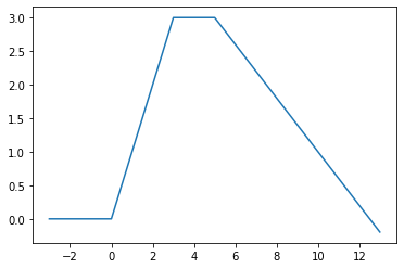
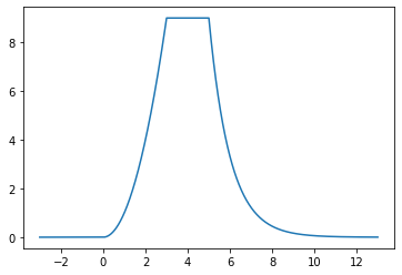
We also compare numerically the approximation properties of deep quadratic neural networks, which is not considered theoretically here. We have chosen two simple test cases of one-dimensional functions (see Figure 3) to approximate, for which we analyze the approximation properties of different neural networks numerically.

Finally, our goal is to extend the basic proof-of-concept examples to some clusterization problems and discuss some real world application examples.

5.1. Proof-of-concept example

5.1.1 Ground Truth Data

We study the numerical approximation of two simple test-data, which are analytically given by

f_{1}(x)=\begin{cases}0&x\leq 0\\ x&0<x\leq 3\\ 3&3<x\leq 5\\ -0.4x+5&5<x\\ \end{cases}\qquad f_{2}(x)=\begin{cases}0&x\leq 0\\ x^{2}&0<x\leq 3\\ 9&3<x\leq 5\\ 9\mathrm{e}^{-(x-5)}&5<x\\ \end{cases}

(5.1)

5.1.2 Generation of training data and initialization

The functions from above were evaluated in $1600$ uniformly distributed points in $[-3,13]$ . The pairs $(x,y)$ of generated data were then randomly split into $1072$ training pairs and $528$ test pairs. In the rest of the paper $f_{2}$ is observed, but the analysis has also been conducted for $f_{1}$ , where the results are similar.

5.1.3 Implementation details

The implementation is based on already implemented methods of TensorFlow [1] and Keras [4], with adaptations - where necessary - to resemble the structure of the decision functions from (3.2). The following pseudocode illustrates the general procedure and highlights custom implemented features.

Structure of an elliptical layer

Inputs:

inputs

\leftarrow

function values of ground truth data

input_dimension

\leftarrow

numer of neurons of input

output_dimension

\leftarrow

number of neurons of output

Variables:

\sigma_{i}

\leftarrow

weights for the ’elliptical’ part (dim of matrix: input dimension

\times

number of neurons)

{\bf{w}}_{1..n}

\leftarrow

weights for the ’affine linear’ part (dim of matrix: input_dimension

\times

number of neurons)

{\bf{w}}_{n+1}

\leftarrow

weight that is multiplied with ’elliptical part’ for each neuron (dim of matrix: 1

\times

number of neurons)

\theta

\leftarrow

bias for each neuron to add to ’affine linear part’ (dim of matrix: 1

\times

number of neurons)

Initialize:

\sigma_{i}

{\bf{w}}_{1..n}

{\bf{w}}_{n+1}

\leftarrow

random gaussian distribution (mean=1.0, stddev=0, seed=None)

\theta

\leftarrow

class Elliptical_layer(input_dimension, output_dimension)

function call(inputs)

outputs

\leftarrow

{\bf{w}}_{1..n}

\cdot

inputs +

{\bf{w}}_{n+1}

\cdot

\sigma_{i}^{2}

\cdot

inputs² +

\theta

store outputs

return outputs

end function

function backprop(labels):

update weights with Adam optimizer

end function

end class

Stacking together different layers and training (Example for a deep neural network)

Initialize:

x_{train},y_{train}

\leftarrow

training data

test_{epochs}

\leftarrow

number of complete pass throughs of the training data

layer_in

\leftarrow

Object of Elliptic class with 1 input,

X_{1}

outputs

layer_hidden_1

\leftarrow

Object of Elliptic class with

X_{1}

input,

Y_{n}

outputs

\vdots

layer_hidden_n

\leftarrow

Object of Elliptic class with

X_{n}

input,

Y_{n}

outputs

layer_out

\leftarrow

Object of Elliptic class with

Y_{n}

input, 1 outputs

network = List(layer_in, layer_hidden_1,

\,\ldots\,

,layer_hidden_n, layer_out)

Output:

\mathrm{network}_{loss}=\textrm{network}.fit(x_{train},y_{train},epochs=test_{epochs})

The implementation in our specific setting has been done for one, three and four hidden layers, but, as the pseudocode demonstrates, it can easily be adapted to neural networks with any number of hidden layers. The Adam optimizer with a learning rate of $0.001$ has been selected as the optimization method of choice. If we determine a bad initialization, it randomly chooses another one and starts again.

The following results shown in the next subsections have all been performed on a 2,4 GHz 8-Core Intel Core i9 processor with 32 GB RAM.

5.1.4 Convergence rates of shallow elliptic networks

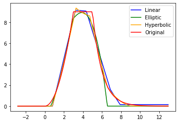
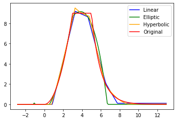
We have varied the number of neurons $N$ to evaluate the convergence rates proven in Section 4.1, which shows the predicted convergence rates of elliptic neural networks (generalization of circular decision functions, which lead to more stable results). The results can be observed in Figure 4.

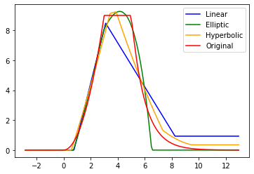
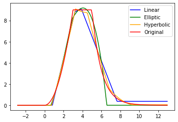
In a next step, the convergence rates of elliptic neural networks should be compared with those of affine linear and hyperbolic ones. The following graph shows the development of the reconstruction each adding up 50 epochs. One epoch describes one complete pass through the training data, as in the Keras library. During each epoch, the weights (including $\sigma_{i}$ ) are updated.

The images in Figure 5 show us, that when one considers training for 50 epochs, only approximation via elliptic (generalization of circular) decision functions performs reasonably well. When using more epochs, hyperbolic and affine linear catches up with elliptic and have a similar approximation error (see also Table 1). Figure 6 provides us with the error function, where it is clearly observable that the elliptic layers converge faster than the affine linear and hyperbolic ones.

The MSE error corresponds with the ${L^{2}}$ -norm from the theoretical section.

Type of network	Training epochs	Hidden layers	Units per hidden layer	Test MSE	Test MAE
Elliptic	250	1	[5]	0.0731	0.2592
Elliptic	140	1	[5]	0.08795	0.25975
Affine Linear	250	1	[5]	0.2008	0.2102
Affine Linear	140	1	[5]	0.47645	0.30545
Hyperbolic	250	1	[5]	0.0574	0.2977
Hyperbolic	140	1	[5]	0.2164	0.3281

Table 1: Overview of the result of the numerical experiments for shallow networks.

Please note, that the approximation with hyperbolic and affine linear layers do not satisfy all proposed conditions on $\sigma$ (see Lemma 4.3).

5.1.5 Deep networks

In this section, we present the error functions for deep neural networks with multiple hidden layers, associated to the pseudocode presented before.

The following results (both in Figure 7 and Figure 8) confirm our hypothesis, that the deep elliptic neural networks converge faster than the affine linear ones. Full results can be observed in Table 2.

Type of network	Training epochs	Hidden layers	Units per hidden layer	Test MSE	Test MAE
Elliptic	140	3	[5, 5, 5]	0.0106	0.1752
	140	3	[30, 30, 30]	0.0014	0.0404
	140	4	[5, 5, 5, 5]	0.0528	0.0767
Affine Linear	140	4	[5,5,5,5]	0.0105	0.2074
Affine Linear	140	4	[30,30,30,30]	0.0453	0.0618

Table 2: Overview of the result of the numerical experiments for deep networks.

5.2. Clusterization examples

In this subsection, we are going to look at a more "applied setting", in detail classification problems.

We will start with the well-known MNIST dataset (see [9]), which is a database consisting out of 60,000 examples of training data as well as 10,000 examples as test data of handwritten digits. The images which were used are size-normalized and centered in a fixed-size image.

Out of these images a t-distributed stochastic neighbour embedding (t-SNE) was generated. This procedure is a machine learning algorithm for dimensionality reduction and often used for visualization purposes. t-SNE preserves local structures of the dataset by letting the distances between points stay the same.

The use case for the quadratic neural networks would be the following: By only having the different clusters, the goal would now be to correctly classify MNIST images of which only the t-SNE embedding is known.

5.2.1 Generation of training data and initialization

The training data is generated via the t-distributed stochastic neighbour of the 60,000 examples - in the following one can see a visualization of it. One sees the clear groups of the different digits. For the test data set, we have generated $10,000$ data points, where the correct classification shall be determined. For means of simplicity, this paper observes the correct clustering of e.g. digit 8.

To determine the correct clustering for the other digits as well, one simply generates additional networks for the classification of the other numbers. When having conducted these experiments, this has increased the performance for the other digits as well. For the generation of the neighbour clustering, we have used code available on Kaggle for the t-sne-visualization.

5.2.2 Results

The following table indicates the advantage of using elliptic (generalization of circular) decision functions and not linear ones. When using more epochs, hyperbolic and affine linear catches up with elliptic and have a similar approximation error (see also Table 3).

We have used different combinations to observe the different outcomes (see Figure 10).

Type	Epochs	H. layers	Units per hidden layer	S. C. Crossentropy
Elliptic	10	1	[5]	0.9515
Elliptic	10	3	[5,5,5]	0.9757
Elliptic	30	3	[20,20,20]	0.9770
Affine Linear	10	1	[5]	0.9033
Affine Linear	10	3	[5,5,5]	0.9570
Affine Linear	30	3	[20,20,20]	0.973

Table 3: Overview of the result of the numerical experiments for deep networks.

5.2.3 Summary and possible extensions

Having also performed other experiments, we can clearly state that there are several cases, under which the use of elliptical layers practically makes sense. Especially, when one is interested into convergence rates, one is obliged to use a small neural network structure (or even shallow neural networks). In such cases, these specially constructed decision functions clearly have an advantage.

In the following analysis, we will discuss the classification on Figure 11 (B) when one sole layer (shallow neural network structure) is used. Via those two "relatively simple" examples, it lets us understand which effect the different layers particularly have from a geometrical point of view. This we will compare with the usage of e.g. classical linear layers. The setting was done similarly as above, we have used for the experiments a shallow neural network structure with 20 epochs of training.

We remember: The subpopulation should be identified out of a much bigger population. As already performed in the previous experiment, one has specific data points given in both the populations.

One sees that the classification via an elliptical layer leads to a loss of 0.004 and an accuracy of 0.998. Therefore this structure can very well classify elliptical data points.

When one e.g. observes the classification via one parabolic layer, the following phenomena occurs:

This is why it makes definite sense to choose a specific layer for a specific application case. This also comes into play when one uses a shallow linear network, which does not lead to reasonably well results.

When using more epochs and more hidden layers, hyperbolic and affine linear catches up with elliptic and have a similar approximation error. A similar result has been observed in the previous experiment.

Figure 15provides us with the accuracy of the elliptic model and Figure 16 the development of the loss function.

6. Conclusion

In this paper we suggested the use of new types of neurons in fully connected neural networks. We proved a universal approximation theorem, which is applicable to such novel networks. Furthermore, we give the explicit convergence rates for the case of circular neurons, which has the same order as the classical affine linear neurons, but with vastly reduced number of neurons (in particular is spares one layer).

Additionally, the numerical results have confirmed the improved convergence for quadratic neural network functions when compared with affine linear ones, not only for three-layer networks, but also for deep neural networks. Potential next steps involve similar analysis for higher order polynomials, as only quadratic neural network functions have been covered in this paper. Furthermore, higher dimension problems are a potential matter of interest in a follow-up paper.

Appendix A Approximation to the identity (AtI)

Definition A.1 (Approximation to the identity [8]).

A sequence of symmetric kernel functions $(S_{k}:\mathbb{R}^{n}\times\mathbb{R}^{n}\to\mathbb{R})_{k\in\mathbb{Z}}$ is said to be an approximation to the identity (AtI) if there exist a quintuple $(\epsilon,\zeta,C,C_{\rho},C_{A})$ of positive numbers satisfying the additional constraints

0<\epsilon\leq\frac{1}{n},0<\zeta\leq\frac{1}{n}\text{ and }C_{A}<1

(A.1)

the following three conditions are satisfied for all $k\in\mathbb{Z}$ :

(i)

$\left|S_{k}({\vec{x}},{\vec{y}})\right|\leq C\frac{2^{-k\epsilon}}{\left(2^{-k}+C_{\rho}\left\|{\vec{x}}-{\vec{y}}\right\|^{n}\right)^{1+\epsilon}}$ for all ${\vec{x}},{\vec{y}}\in\mathbb{R}^{n}$ ;

(ii)

$\left|S_{k}({\vec{x}},{\vec{y}})-S_{k}({\vec{x}}^{\prime},{\vec{y}})\right|\leq C\left(\frac{C_{\rho}\left\|{\vec{x}}-{\vec{x}}^{\prime}\right\|^{n}}{2^{-k}+C_{\rho}\left\|{\vec{x}}-{\vec{y}}\right\|^{n}}\right)^{\zeta}\frac{2^{-k\epsilon}}{\left(2^{-k}+C_{\rho}\left\|{\vec{x}}-{\vec{y}}\right\|^{n}\right)^{1+\epsilon}}$
for all triples $({\vec{x}},{\vec{x}}^{\prime},{\vec{y}})\in\mathbb{R}^{n}\times\mathbb{R}^{n}\times\mathbb{R}^{n}$ which satisfy

C_{\rho}\left\|{\vec{x}}-{\vec{x}}^{\prime}\right\|^{n}\leq C_{A}\left(2^{-k}+C_{\rho}\left\|{\vec{x}}-{\vec{y}}\right\|^{n}\right);

(A.2)

(iii)

$\int_{\mathbb{R}^{n}}S_{k}({\vec{x}},{\vec{y}})d{\vec{y}}=1$ for all ${\vec{x}}\in\mathbb{R}^{n}$ .

Moreover, we say that the AtI satisfies the double Lipschitz condition if there exist a triple $(\tilde{C},\tilde{C}_{A},\zeta)$ of positive constants satisfying

\tilde{C}_{A}<\frac{1}{2},

(A.3)

such that for all $k\in\mathbb{Z}$

		$\displaystyle\left\|S_{k}({\vec{x}},{\vec{y}})-S_{k}({\vec{x}}^{\prime},{\vec{y}})-S_{k}({\vec{x}},{\vec{y}}^{\prime})+S_{k}({\vec{x}}^{\prime},{\vec{y}}^{\prime})\right\|$		(A.4)
	$\displaystyle\leq$	$\displaystyle\tilde{C}\left(\frac{C_{\rho}\left\\|{\vec{x}}-{\vec{x}}^{\prime}\right\\|^{n}}{2^{-k}+C_{\rho}\left\\|{\vec{x}}-{\vec{y}}\right\\|^{n}}\right)^{\zeta}\left(\frac{C_{\rho}\left\\|{\vec{y}}-{\vec{y}}^{\prime}\right\\|^{n}}{2^{-k}+C_{\rho}\left\\|{\vec{x}}-{\vec{y}}\right\\|^{n}}\right)^{\zeta}\frac{2^{-k\epsilon}}{(2^{-k}+C_{\rho}\left\\|{\vec{x}}-{\vec{y}}\right\\|^{n})^{1+\epsilon}}$		(A.4)

for all quadruples $({\vec{x}},{\vec{x}}^{\prime},{\vec{y}},{\vec{y}}^{\prime})\in\mathbb{R}^{n}\times\mathbb{R}^{n}\times\mathbb{R}^{n}\times\mathbb{R}^{n}$ which satisfy

C_{\rho}\max\left\{\left\|{\vec{x}}-{\vec{x}}^{\prime}\right\|^{n},\left\|{\vec{y}}-{\vec{y}}^{\prime}\right\|^{n}\right\}\leq\tilde{C}_{A}\left(2^{-k}+C_{\rho}\left\|{\vec{x}}-{\vec{y}}\right\|^{n}\right).

(A.5)

The conditions item (ii) and Equation A.5 are essential for our analysis. We characterize now geometric properties of these constrained sets:

Lemma A.2.

Let $C_{\rho}=1$ , $C_{A}=2^{-n}$ and $\tilde{C}_{A}=3^{-n}$ .

•

Then set of triples $({\vec{x}},{\vec{x}}^{\prime},{\vec{y}})$ which satisfy Equation A.2 and for which $\left\|{\vec{x}}-{\vec{y}}\right\|^{n}\geq 2^{-k}$ and all $t\in[0,1]$ satisfy

\left\|{\vec{x}}+t({\vec{x}}^{\prime}-{\vec{x}})-{\vec{y}}\right\|^{n}\geq 2^{-n}\left\|{\vec{x}}-{\vec{y}}\right\|^{n}-2^{-n}2^{-k}.

(A.6)

•

The set of quadrupels $({\vec{x}},{\vec{x}}^{\prime},{\vec{y}},{\vec{y}}^{\prime})$ which satisfy Equation A.5 and for which $\left\|{\vec{x}}-{\vec{y}}\right\|^{n}\geq 2^{-k}$ satisfy

\left\|{\vec{x}}+t_{\vec{x}}({\vec{x}}^{\prime}-{\vec{x}})-{\vec{y}}-t_{\vec{y}}({\vec{y}}^{\prime}-{\vec{y}})\right\|^{n}\geq 3^{-n}\left\|{\vec{x}}-{\vec{y}}\right\|^{n}-3^{-n}2^{1-k}

(A.7)

for all $t_{\vec{x}},t_{\vec{y}}\in[0,1]$ .

Proof.

•

With the concrete choice of parameters $C_{A}$ , $C_{\rho}$ Equation A.2 reads as follows

\left\|{\vec{x}}-{\vec{x}}^{\prime}\right\|^{n}\leq 2^{-n}\left(2^{-k}+\left\|{\vec{x}}-{\vec{y}}\right\|^{n}\right).

(A.8)

Since we assume that $\left\|{\vec{x}}-{\vec{y}}\right\|^{n}\geq 2^{-k}$ it follows from Equation A.8 that

\left\|{\vec{x}}-{\vec{x}}^{\prime}\right\|\leq 2^{-1}\left\|{\vec{x}}-{\vec{y}}\right\|.

In particular $\left\|{\vec{x}}-{\vec{y}}\right\|-\left\|{\vec{x}}-{\vec{x}}^{\prime}\right\|\geq 0$ .

We apply Jensen’s inequality, which states that for $a,b\geq 0$

a^{n}+b^{n}\geq 2^{1-n}(a+b)^{n}.

(A.9)

We use $a=\left\|{\vec{x}}+t({\vec{x}}^{\prime}-{\vec{x}})-{\vec{y}}\right\|$ and $b=\left\|t({\vec{x}}^{\prime}-{\vec{x}})\right\|$ , which then (along with the triangle inequality) gives

\left\|{\vec{x}}+t({\vec{x}}^{\prime}-{\vec{x}})-{\vec{y}}\right\|^{n}+\left\|t({\vec{x}}^{\prime}-{\vec{x}})\right\|^{n}\geq 2^{1-n}\left(\left\|{\vec{x}}-{\vec{y}}\right\|\right)^{n}.

In other words, it follows from Equation A.8 that

	$\displaystyle\left\\|{\vec{x}}+t({\vec{x}}^{\prime}-{\vec{x}})-{\vec{y}}\right\\|^{n}$	$\displaystyle\geq 2^{1-n}\left\\|{\vec{x}}-{\vec{y}}\right\\|^{n}-t^{n}\left\\|{\vec{x}}^{\prime}-{\vec{x}}\right\\|^{n}$
		$\displaystyle\geq 2^{1-n}\left\\|{\vec{x}}-{\vec{y}}\right\\|^{n}-\left\\|{\vec{x}}^{\prime}-{\vec{x}}\right\\|^{n}$
		$\displaystyle\geq 2^{1-n}\left\\|{\vec{x}}-{\vec{y}}\right\\|^{n}-2^{-n}\left(2^{-k}+\left\\|{\vec{x}}-{\vec{y}}\right\\|^{n}\right)$
		$\displaystyle=2^{-n}\left\\|{\vec{x}}-{\vec{y}}\right\\|^{n}-2^{-n}2^{-k}.$

•

With the concrete choice of parameters $\tilde{C}_{A}$ , $C_{\rho}$ Equation A.5 reads as follows

\max\left\{\left\|{\vec{x}}-{\vec{x}}^{\prime}\right\|^{n},\left\|{\vec{y}}-{\vec{y}}^{\prime}\right\|^{n}\right\}\leq 3^{-n}\left(2^{-k}+\left\|{\vec{x}}-{\vec{y}}\right\|^{n}\right).

(A.10)

Since we assume that $\left\|{\vec{x}}-{\vec{y}}\right\|^{n}\geq 2^{-k}$ it follows from Equation A.10 that

\max\left\{\left\|{\vec{x}}-{\vec{x}}^{\prime}\right\|,\left\|{\vec{y}}-{\vec{y}}^{\prime}\right\|\right\}\leq 3^{-1}\left\|{\vec{x}}-{\vec{y}}\right\|.

This in particular shows that

\left\|{\vec{x}}-{\vec{y}}\right\|-\left\|{\vec{x}}-{\vec{x}}^{\prime}\right\|-\left\|{\vec{y}}-{\vec{y}}^{\prime}\right\|\geq 0.

We apply Jensen’s inequality, which states that for $a,b,c\geq 0$

a^{n}+b^{n}+c^{n}\geq 3^{1-n}(a+b+c)^{n}.

(A.11)

We use $a=\left\|{\vec{x}}+t_{\vec{x}}({\vec{x}}^{\prime}-{\vec{x}})-{\vec{y}}-t_{\vec{y}}({\vec{y}}^{\prime}-{\vec{y}})\right\|$ , $b=\left\|t_{\vec{x}}({\vec{x}}^{\prime}-{\vec{x}})\right\|$ and $c=\left\|t_{\vec{y}}({\vec{y}}^{\prime}-{\vec{y}})\right\|$ , which then (along with the triangle inequality) gives

\left\|{\vec{x}}+t_{\vec{x}}({\vec{x}}^{\prime}-{\vec{x}})-{\vec{y}}-t_{\vec{y}}({\vec{y}}^{\prime}-{\vec{y}})\right\|^{n}+\left\|t_{\vec{x}}({\vec{x}}^{\prime}-{\vec{x}})\right\|^{n}+\left\|t_{\vec{y}}({\vec{y}}^{\prime}-{\vec{y}})\right\|^{n}\geq 3^{1-n}\left\|{\vec{x}}-{\vec{y}}\right\|^{n}.

In other words, it follows from Equation A.10 that

	$\displaystyle\left\\|{\vec{x}}+t_{\vec{x}}({\vec{x}}^{\prime}-{\vec{x}})-{\vec{y}}-t_{\vec{y}}({\vec{y}}^{\prime}-{\vec{y}})\right\\|^{n}$	$\displaystyle\geq 3^{1-n}\left\\|{\vec{x}}-{\vec{y}}\right\\|^{n}-t_{\vec{x}}^{n}\left\\|{\vec{x}}^{\prime}-{\vec{x}}\right\\|^{n}-t_{\vec{y}}^{n}\left\\|{\vec{y}}^{\prime}-{\vec{y}}\right\\|^{n}$
		$\displaystyle\geq 3^{1-n}\left\\|{\vec{x}}-{\vec{y}}\right\\|^{n}-\left\\|{\vec{x}}^{\prime}-{\vec{x}}\right\\|^{n}-\left\\|{\vec{y}}^{\prime}-{\vec{y}}\right\\|^{n}$
		$\displaystyle\geq 3^{1-n}\left\\|{\vec{x}}-{\vec{y}}\right\\|^{n}-3^{-n}2\left(2^{-k}+\left\\|{\vec{x}}-{\vec{y}}\right\\|^{n}\right)$
		$\displaystyle=3^{-n}\left\\|{\vec{x}}-{\vec{y}}\right\\|^{n}-3^{-n}2^{1-k}.$

$\square$

The approximation to the identity in Appendix A can be used to construct wavelet frames that can approximate arbitrary functions in $\mathcal{L}^{1}(\mathbb{R}^{n})$ , as shown in the theorem below.

Remark 5.

When $\left\|{\vec{x}}-{\vec{y}}\right\|^{n}<2^{-k}$ , Equation A.6 also holds since the right hand side of Equation A.6 is negative, so this inequality is trivial.

Theorem A.3 ([23]).

Let $(S_{k}:\mathbb{R}^{n}\times\mathbb{R}^{n}\to\mathbb{R})_{k\in\mathbb{Z}}$ be a symmetric AtI which satisfies the double Lipschitz condition (see Equation A.4). Let

\psi_{k,{\vec{y}}}({\vec{x}}):=2^{-\frac{k}{2}}\left(S_{k}({\vec{x}},{\vec{y}})-S_{k-1}({\vec{x}},{\vec{y}})\right)\text{ for all }{\vec{x}},{\vec{y}}\in\mathbb{R}^{n}\text{ and }k\in\mathbb{Z}.

(A.12)

The the set of functions

\mathcal{F}:=\left\{{\vec{x}}\to\psi_{k,b}({\vec{x}}):k\in\mathbb{Z},b\in 2^{-\frac{k}{d}}\mathbb{Z}\right\},

(A.13)

is a frame and for every function $f\in\mathcal{L}^{1}(\mathbb{R}^{n})$ there exists a linear combination of $N$ elements of $\mathcal{F}$ , denoted by $f_{N}$ , satisfying

\left\|f-f_{N}\right\|_{L^{2}}\leq\left\|f\right\|_{\mathcal{L}^{1}}(N+1)^{-1/2}.

Acknowledgements

OS is supported by the Austrian Science Fund (FWF), with SFB F68, project F6807-N36 - Tomography with Uncertainties. LF is supported by the Austrian Science Fund (FWF) with SFB F68, project F6807-N36 (Tomography with Uncertainties). CS is supported by the Austrian Science Fund (FWF), with project AT0116011 (Photoacoustic tomography: analysis and numerics). The financial support by the Austrian Federal Ministry for Digital and Economic Affairs, the National Foundation for Research, Technology and Development and the Christian Doppler Research Association is gratefully acknowledged.

References

[1] M. Abadi et al. “TensorFlow: Large-Scale Machine Learning on Heterogeneous Systems” In arXiv, 2021 URL: https://arxiv.org/abs/1603.04467
[2] A.. Barron “Universal approximation bounds for superpositions of a sigmoidal function” In IEEE Transactions on Information Theory 39.3, 1993, pp. 930–945 DOI: 10.1109/18.256500
[3] A.. Barron, A. Cohen, W. Dahmen and R.. DeVore “Approximation and learning by greedy algorithms” In Annals of Statistics 36.1, 2008 DOI: 10.1214/009053607000000631
[4] F. Chollet “Keras”, 2015 URL: https://keras.io
[5] O. Christensen “An Introduction to Frames and Riesz Bases” Springer International Publishing, 2016 DOI: 10.1007/978-3-319-25613-9
[6] G. Cybenko “Approximation by superpositions of a sigmoidal function” In Mathematics of Control, Signals, and Systems 2.4, 1989, pp. 303–314 DOI: 10.1007/bf02551274
[7] K. Deimling “Nonlinear Functional Analysis”, 1985 DOI: 10.1007/978-3-662-00547-7
[8] D. Deng and Y. Han “Harmonic Analysis on Spaces of Homogeneous Type” Springer Berlin Heidelberg, 2009 DOI: 10.1007/978-3-540-88745-4
[9] Li Deng “The mnist database of handwritten digit images for machine learning research” In IEEE Signal Processing Magazine 29.6 IEEE, 2012, pp. 141–142
[10] J. Dugundji “Topology” Reprinting of the 1966 original AllynBacon, Inc., 1978
[11] F. Fan, J. Xiong and G. Wang “Universal approximation with quadratic deep networks” In Neural Networks 124, 2020, pp. 383–392 DOI: 10.1016/j.neunet.2020.01.007
[12] E. Gelenbe, Zhi-Wong Mao and Yan-Da Li “Approximation by random networks with bounded number of layers” In Neural Networks for Signal Processing IX: Proceedings of the 1999 IEEE Signal Processing Society Workshop (Cat. No.98TH8468), 1999 DOI: 10.1109/nnsp.1999.788135
[13] B. Hammer “Learning with Recurrent Neural Networks”, Lecture Notes in Control and Information Sciences Springer London, 2000 URL: https://books.google.li/books?id=8IjKhLs8siwC
[14] K. Hornik, M. Stinchcombe and H. White “Multilayer feedforward networks are universal approximators” In Neural Networks 2.5, 1989, pp. 359–366 DOI: 10.1016/0893-6080(89)90020-8
[15] B. Igelnik and Y. Pao “Stochastic choice of basis functions in adaptive function approximation and the functional-link net” In IEEE Transactions on Neural Networks 6.6, 1995, pp. 1320–1329 DOI: 10.1109/72.471375
[16] J.. Kelley “General Topology” Toronto-New York-London: D. Van Nostrand Company, 1955
[17] M. Leshno, V.. Lin, A. Pinkus and S. Schocken “Multilayer feedforward networks with a nonpolynomial activation function can approximate any function” In Neural Networks 6.6, 1993, pp. 861–867 DOI: 10.1016/s0893-6080(05)80131-5
[18] O. Manita et al. “Universal Approximation in Dropout Neural Networks” In Journal of Machine Learning Research 23.19, 2022, pp. 1–46 URL: http://jmlr.org/papers/v23/20-1433.html
[19] H.. Mhaskar “Approximation properties of a multilayered feedforward artificial neural network” In Advances in Computational Mathematics 1.1 Springer US, 1993, pp. 61–80 DOI: 10.1007/bf02070821
[20] Y.-H. Pao, G.-H. Park and D.. Sobajic “Learning and generalization characteristics of the random vector functional-link net” In Neurocomputing 6.2, 1994, pp. 163–180 DOI: 10.1016/0925-2312(94)90053-1
[21] A. Pinkus “Approximation theory of the MLP model in neural networks” In Acta Numerica 8, 1999, pp. 143–195 DOI: 10.1017/s0962492900002919
[22] A. Sch\"afer and H. Zimmermann “Recurrent Neural Networks are universal approximators” In International Journal of Neural Systems 17.04, 2007, pp. 253–263 DOI: 10.1142/S0129065707001111
[23] U. Shaham, A. Cloninger and R.. Coifman “Provable approximation properties for deep neural networks” In Applied and Computational Harmonic Analysis 44.3, 2018, pp. 537–557 DOI: 10.1016/j.acha.2016.04.003
[24] N. Tsapanos, A. Tefas, N. Nikolaidis and I. Pitas “Neurons With Paraboloid Decision Boundaries for Improved Neural Network Classification Performance” In IEEE Transactions on Neural Networks and Learning Systems 30.1, 2019, pp. 284–294 DOI: 10.1109/TNNLS.2018.2839655
[25] S Wager, S Wang and P Liang “Dropout Training as Adaptive Regularization” In Proceedings of the 26th International Conference on Neural Information Processing Systems - Volume 1 Curran Associates Inc., 2013, pp. 351–359
[26] White “An additional hidden unit test for neglected nonlinearity in multilayer feedforward networks” In International Joint Conference on Neural Networks, 1989 DOI: 10.1109/ijcnn.1989.118281
[27] D.-X. Zhou “Deep distributed convolutional neural networks: Universality” In Analysis and Applications 16.6, 2018, pp. 895–919 DOI: 10.1142/s0219530518500124
[28] D.-X. Zhou “Universality of deep convolutional neural networks” In Applied and Computational Harmonic Analysis 48.2, 2020, pp. 787–794 DOI: 10.1016/j.acha.2019.06.004

	$\displaystyle\left\\|\nabla_{\vec{x}}(S_{k}({\vec{x}},{\vec{y}}))\right\\|$	$\displaystyle=\left\\|\nabla_{\vec{x}}(2^{k}\varphi(2^{\frac{k}{n}}({\vec{x}}-{\vec{y}})))\right\\|=2^{k}\left\\|\nabla_{\vec{x}}S_{0}(2^{\frac{k}{n}}{\vec{x}},2^{\frac{k}{n}}{\vec{y}})\right\\|=2^{k+\frac{k}{n}}F_{2^{\frac{k}{n}}{\vec{y}}}(2^{\frac{k}{n}}{\vec{x}})$		(4.7)
		$\displaystyle\leq 2^{-\frac{k}{n}}C_{d}C_{\sigma}(2^{-k}+\left\\|{\vec{x}}-{\vec{y}}\right\\|^{n})^{-1-\frac{2}{n}}.$		(4.7)

$\displaystyle\frac{\left\|S_{k}({\vec{x}},{\vec{y}})-S_{k}({\vec{x}}^{\prime},{\vec{y}})\right\|}{\left\\|{\vec{x}}-{\vec{x}}^{\prime}\right\\|}$	$\displaystyle\leq\max_{\left\{\vec{z}=t{\vec{x}}^{\prime}+(1-t){\vec{x}}:t\in[0,1]\right\}}\left\\|\nabla_{\vec{x}}(S_{k}(\vec{z},{\vec{y}}))\right\\|$	(4.8)
	$\displaystyle\leq 2^{-\frac{k}{n}}C_{d}C_{\sigma}\max_{\left\{\vec{z}={\vec{x}}+t({\vec{x}}^{\prime}-{\vec{x}}):t\in[0,1]\right\}}(2^{-k}+\left\\|\vec{z}-{\vec{y}}\right\\|^{n})^{-1-\frac{2}{n}}$
	$\displaystyle=2^{-\frac{k}{n}}C_{d}C_{\sigma}\left(2^{-k}+\min_{\left\{\vec{z}={\vec{x}}+t({\vec{x}}^{\prime}-{\vec{x}}):t\in[0,1]\right\}}\left\\|\vec{z}-{\vec{y}}\right\\|^{n}\right)^{-1-\frac{2}{n}}.$

	$\displaystyle\frac{\left\|S_{k}({\vec{x}},{\vec{y}})-S_{k}({\vec{x}}^{\prime},{\vec{y}})\right\|}{\left\\|{\vec{x}}-{\vec{x}}^{\prime}\right\\|}$	$\displaystyle\leq 2^{-\frac{k}{n}}C_{d}C_{\sigma}\left((1-2^{-n})2^{-k}+2^{-n}\left\\|{\vec{x}}-{\vec{y}}\right\\|^{n}\right)^{-1-\frac{2}{n}}$
		$\displaystyle\leq 2^{-\frac{k}{n}}\left(2^{-n}\right)^{-1-\frac{2}{n}}C_{d}C_{\sigma}\left(\frac{(1-2^{-n})}{2^{-n}}2^{-k}+\left\\|{\vec{x}}-{\vec{y}}\right\\|^{n}\right)^{-1-\frac{2}{n}}$
		$\displaystyle\leq 2^{-\frac{k}{n}}2^{n+2}C_{d}C_{\sigma}\left(2^{-k}+\left\\|{\vec{x}}-{\vec{y}}\right\\|^{n}\right)^{-1-\frac{2}{n}}.$

	$\displaystyle\left\\|\nabla^{2}_{{\vec{x}}{\vec{y}}}S_{k}(\vec{z}^{\prime},\vec{z})\right\\|\leq$	$\displaystyle 2^{2}2^{k+2\frac{k}{n}}C_{d}C_{\sigma}\max\left\{2\left\\|\vec{\omega}\right\\|^{2}(1+\left\\|\vec{\omega}\right\\|^{n})^{-1-\frac{5}{n}},(1+\left\\|\vec{\omega}\right\\|^{n})^{-1-\frac{3}{n}}\right\}$
	$\displaystyle\leq$	$\displaystyle 2^{3}2^{k+2\frac{k}{n}}C_{d}C_{\sigma}(1+\left\\|\vec{\omega}\right\\|^{n})^{-1-\frac{3}{n}}$
	$\displaystyle\leq$	$\displaystyle 2^{-\frac{k}{n}}2^{3}C_{d}C_{\sigma}(2^{-k}+\left\\|\vec{z}^{\prime}-\vec{z}\right\\|^{n})^{-1-\frac{3}{n}}.$

		$\displaystyle\frac{\left\|S_{k}({\vec{x}},{\vec{y}})-S_{k}({\vec{x}}^{\prime},{\vec{y}})-S_{k}({\vec{x}},{\vec{y}}^{\prime})+S_{k}({\vec{x}}^{\prime},{\vec{y}}^{\prime})\right\|}{\left\\|{\vec{x}}-{\vec{x}}^{\prime}\right\\|\left\\|{\vec{y}}-{\vec{y}}^{\prime}\right\\|}$
	$\displaystyle\leq$	$\displaystyle 2^{-\frac{k}{n}}2^{3}C_{d}C_{\sigma}\left((1-3^{-n}2)2^{-k}+3^{-n}\left\\|{\vec{x}}-{\vec{y}}\right\\|^{n}\right)^{-1-\frac{3}{n}}$
	$\displaystyle\leq$	$\displaystyle 2^{-\frac{k}{n}}2^{3}(3^{-n})^{-1-\frac{3}{n}}C_{d}C_{\sigma}\left(\frac{1-3^{-n}2}{3^{-n}}2^{-k}+\left\\|{\vec{x}}-{\vec{y}}\right\\|^{n}\right)^{-1-\frac{3}{n}}$
	$\displaystyle\leq$	$\displaystyle 2^{-\frac{k}{n}}2^{3}3^{n+3}C_{d}C_{\sigma}\left(2^{-k}+\left\\|{\vec{x}}-{\vec{y}}\right\\|^{n}\right)^{-1-\frac{3}{n}}.$

Approximation properties of shallow quadratic neural networks and clustering applications

Abstract

1. Introduction

2. Generalized universal approximation theorem

Notation 2.1 (Vectors).

Notation 2.2 (ℒ1\mathcal{L}^{1} space).

Definition 2.3 (Discriminatory function).

Example 2.4.

Theorem 2.5 ([6]).

Definition 2.6 (mm-dimensional universal approximation functions).

Theorem 2.7 (Generalized universal approximation theorem).

Proof.

3. Universal approximation theorem with quadratic functions

Example 3.1 (Affine linear decision functions).

Definition 3.2 (Quadratic decision functions).

Remark 1.

Corollary 3.3 (Universal approximation of quadratic decision functions).

4. Convergence rates for universal approximation of circular decision functions

Definition 4.1 (Circular wavelet frame).

Remark 2.

4.1. Convergence rates of nets of circular decision function

Lemma 4.2.

Proof.

Lemma 4.3.

Proof.

Remark 3.

Theorem 4.4 (ℒ1\mathcal{L}^{1}-convergence).

Proof.

Remark 4.

5. Numerical experiments

5.1. Proof-of-concept example

5.1.1 Ground Truth Data

5.1.2 Generation of training data and initialization

5.1.3 Implementation details

5.1.4 Convergence rates of shallow elliptic networks

5.1.5 Deep networks

5.2. Clusterization examples

5.2.1 Generation of training data and initialization

5.2.2 Results

5.2.3 Summary and possible extensions

6. Conclusion

Appendix A Approximation to the identity (AtI)

Definition A.1 (Approximation to the identity [8]).

Lemma A.2.

Proof.

Remark 5.

Theorem A.3 ([23]).

Acknowledgements

References

References

Notation 2.2 ( $\mathcal{L}^{1}$ space).

Definition 2.6 ( $m$ -dimensional universal approximation functions).

Theorem 4.4 ( $\mathcal{L}^{1}$ -convergence).