3LegRace: Privacy-Preserving DNN Training over TEEs and GPUs

Based on the capabilities of common TEE platforms such as Intel SGX [6], we consider the following threat model. 1) An adversary may compromise the OS where the TEE is running. However, it cannot breach the TEE environment, 2) the adversary may access hardware disk, runtime stack, memory outside TEEs and communication between trusted and untrusted environments, 3) the adversary may obtain the model parameters and the gradients during training and then analyze underlying relations with the training data, 4) the adversary may obtain data in untrusted environments and infer information in training data, and 5) the adversary may gain some knowledge of the training dataset (e.g., labels), and use public/online resources to improve its attack performance.

AsymML decomposes compute-intensive and memory-intensive modules, especially convolutional layers in modern DNNs [1, 2], and then assigns each part to a suitable platform. At a high level, AsymML starts with decomposing a convolutional layer such that the computation involving privacy-sensitive information is performed in TEEs while the residual part is offloaded to GPUs. Specifically, the input of a convolutional layer denoted by $X$ is decomposed into a low-rank part $X^{\text{(T)}}$ and a residual part $X^{\text{(U)}}$ as shown in Fig. 2. The residual part $X^{\text{(U)}}$ is then protected by adding a small noise as we discuss in Section 4 to ensure privacy.
When the convolutions in GPUs and TEEs are completed, outputs from GPUs denoted by $Y^{\text{(U)}}$ are merged into TEEs denoted by $Y^{\text{(T)}}$, and then followed by a non-linear layer (a pooling layer might be also needed). Outputs after a non-linear layer will be then re-decomposed before proceeding to the next convolution layer. During the whole forward/backward pass, the low-rank part in TEEs is never exposed, which effectively prevents crucial parts of data from being leaked.

We now explain the decomposition in detail. For a convolutional layer with input $X\in\mathbb{R}^{N\times h\times w}$ and kernels $W\in\mathbb{R}^{M\times N\times k\times k}$, where $N$ and $M$ are the number of input and output channels, and $h,w$ and $k$ are the size of inputs and kernels respectively, the $i$-th output channel is computed as follows¹¹ 1 The batch size and the bias are omitted here for simplicity.

By splitting the input $X$ into $X^{\text{(T)}}$ and $X^{\text{(U)}}$, AsymML decomposes the convolution into a trusted convolution $\text{Conv}_{\text{T}}$ and an untrusted convolution $\text{Conv}_{\text{U}}$ as follows

• –

  Forward. During a forward pass, the outputs in TEEs are calculated as follows

  $$\begin{split}Y^{\text{(T)}}_{i}&=\sum_{j=1}^{N}X^{\text{(T)}}_{j}\circledast W_{i,j}=\sum_{j=1}^{N}\sum_{p=1}^{\mathcal{R}}a_{j,p}X^{{}^{\prime}}_{p}\circledast W_{i,j}\\ &=\sum_{p=1}^{\mathcal{R}}X^{{}^{\prime}}_{p}\circledast\sum_{j=1}^{N}a_{j,p}W_{i,j}\equiv\sum_{p=1}^{\mathcal{R}}X^{{}^{\prime}}_{p}\circledast W_{i,p}^{{}^{\prime}},\end{split}$$

  (7)

  where $W_{i,p}^{{}^{\prime}}=\sum_{j=1}^{N}a_{j,p}W_{i,j}$. According to Eq. (7), $\text{Conv}_{\text{T}}$ essentially is a convolution operation with $\mathcal{R}$ input channels, and the kernels $W^{{}^{\prime}}$ that are obtained by regrouping $W$.

• –

  Backward. During a backward pass, given gradient $\nabla_{Y}\mathcal{L}$, $\nabla_{W_{i,j}}^{\text{(T)}}\mathcal{L}$ in TEEs is computed as

  $$\begin{split}\nabla_{W_{i,j}}^{\text{(T)}}\mathcal{L}&=X^{\text{(T)}}_{j}\circledast\nabla_{Y_{i}}\mathcal{L}=\sum_{p=1}^{\mathcal{R}}a_{j,p}\cdot X^{{}^{\prime}}_{p}\circledast\nabla_{Y_{i}}\mathcal{L},\end{split}$$

  (8)

  where $X^{{}^{\prime}}_{p}\circledast\nabla_{Y_{i}}\mathcal{L}$ for $p=1,2,\cdots,\mathcal{R}$ are first computed. $\nabla_{W_{i,j}}^{\text{(T)}}\mathcal{L}$ is obtained by a simple linear transformation with $a_{j,p}$. Hence, the computation complexity of backward passes also depends on $\mathcal{R}$.
  On the other hand, the untrusted forward output $Y^{\text{(U)}}_{i}$ and the backward gradient $\nabla_{W_{i,j}}^{\text{(U)}}\mathcal{L}$ in GPUs are the same as in the classical convolutional layers but with a different input $\mathcal{M}(X^{\text{(U)}})$. The final result $Y_{i}$ and $\nabla_{W_{i,j}}\mathcal{L}$ are obtained by simply adding the results of the TEEs and the GPUs. In addition, as computing $\nabla_{X}\mathcal{L}$ does not involve the input $X$, it is offloaded onto GPUs.

Performing exact SVD on $X\in\mathbb{R}^{N\times h\times w}$ incurs a significant complexity of $O(Nh^{2}w^{2}+N^{2}hw)$, which goes against our objective of reducing the complexity in TEEs. To reduce the complexity, we propose a lightweight SVD approximation that reduces complexity to only $O(\mathcal{R}Nhw)$.

SVD essentially is an algorithm that finds two vectors $\bm{u}^{(i)}$ and $\bm{v}^{(i)}$ to minimize $\left\|\overline{X}^{(i-1)}-\bm{u}^{(i)}\cdot{\bm{v}^{(i)}}^{*}\right\|_{F}$, where $\overline{X}^{(i-1)}$ is the remaining $\overline{X}$ with $i-1$ most principal components extracted. $\left\{\bm{u}^{(i)}\right\}_{i=1}^{hw}$ and $\left\{\bm{v}^{(i)}\right\}_{i=1}^{N}$ are both orthogonal set of vectors. AsymML, however, does not require such orthogonality. Therefore, SVD can be then relaxed as

The computation and memory costs in TEEs are of great concern as they decide AsymML’s performance in a heterogeneous system. In this section, we break down these costs and compare the costs in TEEs and GPUs.

Figure 3 shows computation and memory costs in TEEs and GPUs for the case where $\mathcal{R}/N=1/16$. As described in Section 3.2, the computation complexity of $\text{Conv}_{\text{T}}$ in TEEs increases with the number of principal channels $\mathcal{R}$, while the complexity of $\text{Conv}_{\text{U}}$ in GPUs is the same as that of the original convolutional layer. In addition to $\text{Conv}_{\text{T}}$, all element-wise operations (ReLU, Pooling, etc) and the lightweight SVD are performed in TEEs. As for the memory cost, the inputs and outputs of all element-wise operations are stored in TEEs, together with the inputs $X^{\text{(T)}}$ and the outputs of the convolution $\text{Conv}_{\text{T}}$, $Y^{\text{(T)}}$. On the other hand, inputs $\mathcal{M}(X^{\text{(U)}})$, outputs $Y^{\text{(U)}}$ of $\text{Conv}_{\text{U}}$ and the corresponding gradients $\nabla_{X}\mathcal{L}$ and $\nabla_{Y}\mathcal{L}$ are stored in GPUs.

We first define a metric termed as SVD-channel entropy to formally quantify the low-rank structure in the intermediate features. Then, we show how the SVD-channel entropy changes in a DNN model after each layer. Inspired by SVD entropy [18] and Rényi entropy [19], we define SVD-channel entropy based on singular values obtained in (3). Given the singular values $\left\{s_{p}(X)|\ p=1,\cdots,N\right\}$ of an input matrix $X$ with $N$ channels, the SVD-channel entropy of $X$, denoted by $\mu_{X}$, is defined as follows.

SVD-Channel Entropy in CNNs – In DNNs, given input data with low-rank structure, it is crucial to measure how such structure (measured using SVD-channel entropy) changes after every layer so that we can systematically set the number of principal channels in TEEs. In CNNs, convolutional, batch normalization, pooling and non-linear layers such as ReLU are the basic layers. In this section, we mainly analyze how these basic operators change the structure of the data. All proofs are provided in Appendix A.

For a convolutional layer with a $k\times k$ kernel, it can be viewed as a $1\times 1$ convolutional layer with $k^{2}$ different “input channels". Each “input channel" is a patch of $X_{j}$, denoted as $\left\{\hat{X}_{j,q,r}|1\leq q,r\leq k\right\}$, as shown in Figure 4. Given $X\in R^{N\times h\times w}$, $W\in R^{M\times N\times k\times k}$, the $i$-th output channel can be rewritten as follows

where $W_{i,j,q,r}$ is a $1\times 1$ kernel after this conversion.
Therefore, a $k\times k$ convolution with $N$ input channels is equivalent to a $1\times 1$ convolution with $N\cdot k^{2}$ “input channels": $\left\{\hat{X}_{j,q,r}|1\leq j\leq N,1\leq q,r\leq k\right\}$. To simplify the notation, we denote $\hat{X}_{:,q,r}$ as the $(q,r)$-th patch of all channels, and $\hat{X}_{j,:,:}$ as all patches of the $j$-th channel.

We now show in Theorem 3 that, knowing the SVD-channel entropy of $\hat{X}_{j,:,:}$ for $j=1,\cdots,N$, the SVD-channel entropy of the outputs with $k\times k$ convolution can be accordingly bounded.

Based on Theorem 3, with $k\times k$ kernels, the SVD-channel entropy of the outputs increases with $\mu_{\hat{X}_{j,:,:}}$ for $j=1,\cdots,\mathcal{R}$. Intuitively, if $k$ is larger, more patches are included, then $\mu_{\hat{X}_{j,:,:}}$ will be higher. More numerical analyses are presented in Section 6.2.

BatchNorm layer – Batch normalization is commonly used in CV models to reduce the internal covariate shift. According to Theorem 4, the SVD-channel entropy of outputs is almost the same as that of inputs in a BatchNorm layer.

Hence, the low-rank structure of inputs is still preserved after batch normalization.

ReLU layer – As a non-linear layer, ReLU is the most commonly used operator in DNNs. Theoretically bounding the SVD-channel entropy after ReLU is infeasible. Instead, we empirically measure the SVD-channel entropy after a ReLU in Appendix C and show that the ReLU layers also preserve the low-rank structure.

Pooling layer – Pooling operations include max and average pooling. Max pooling is a also non-linear operator. Similarly, we provide an empirical experiment that shows that a max pooling layer does not greatly change the low-rank structure either (See Appendix C). Besides, the max and the average pooling layers usually deliver similar performance. As stated in Theorem 5, the SVD-channel entropy after an average pooling layer is less than the one before pooling. Therefore, pooling layers still preserve the low-rank structure.

We now provide the DP guarantee of AsymML. AsymML adds a small Gaussian noise to $X^{\text{(U)}}$ to ensure privacy. While the data stored in TEEs are protected by a secure hardware, the Gaussian mechanism further protects the information in the GPUs.

First, for a dataset $\mathcal{X}=\left\{X^{1},X^{2},\cdots,X^{i},\cdots,X^{B}\right\}$, we define the neighboring dataset $\mathcal{X}^{{}^{\prime}}=\left\{X^{1},X^{2},\cdots,0,\cdots,X^{B}\right\}$ for any possible $i$-th record removed [4]. During training, we sample a batch $\mathcal{S}\in\mathcal{X}$ with size $b$. The $\ell_{2}$-sensitivity of the lightweight SVD is given by $\Delta_{2}=\sup_{\mathcal{X},\mathcal{X}^{{}^{\prime}}}\left\|\mathcal{X}^{(U)}-\mathcal{X}^{{}^{\prime}(U)}\right\|\leq\xi\sup_{i}\left\|X^{i}\right\|$, where $\xi$ is the upper bound of the ratio between the Frobenius norms of $X^{\text{(U)}}$ and $X$. Theorem 6 states that AsymML is $(\epsilon,\delta)$-differentially private when a Gaussian noise $\mathcal{N}(0,2\Delta^{2}_{2}\ln{(1.25q/\delta)}/\epsilon^{2}.I)$ is added, where $q=b/B$ is the sampling probability and $I$ is the identity matrix.

We now consider the model inversion attack.

Assumptions – We assume that the attacker has access to the target model $\mathcal{M}_{\text{t}}$. Further, the attacker uses the noisy residuals $\mathcal{M}(\mathcal{X}^{(U)})$ as prior information to help reconstruct the training dataset $\mathcal{X}_{\text{t}}$. In addition, the attacker knows general information such as label information. Therefore, it can find relevant resources (e.g. online images) to learn the target data distribution.

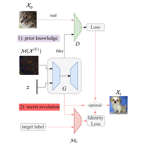
We design the attacker as shown in Fig. 5(a) and Fig. 5(b). Specifically, the attack has two stages as follows.

1. 1.

   Prior Knowledge Distillation. In this stage, the attacker trains a generative adversarial network (GAN) with the public prior knowledge $\mathcal{Z}_{\text{p}}$.

   Fig. 5(b) shows the generator $G$ architecture. It consists of two branches. The first branch B1 is used for learning features from the residual noisy data $\mathcal{M}(\mathcal{X}^{(U)})$. The second branch B2 is used for generating latent features. On the other hand, the discriminator $D$ is a classical CNN. The detailed architectures are provided in Appendix B. The Wasserstein-GAN loss function is used during training as follows

   	$\displaystyle\min_{G}\max_{D}L(G,D)$	$\displaystyle=E_{x\in\mathcal{X}_{\text{p}}}[D(x)]-$
   		$\displaystyle E_{z}[D(G(z,\mathcal{M}(\mathcal{X}^{(U)})))].$		(12)

2. 2.

   Secret Revelation. In this stage, with the noisy residual data $\mathcal{M}(\mathcal{X}^{(U)})$ from the target dataset $\mathcal{X}_{\text{t}}$ along with the labels, the attacker uses the generator to reconstruct images that achieve the highest accuracy in the target model $\mathcal{M}_{\text{t}}$.

   We find the optimal latent vector $z$ that generates an almost-real image to the discriminator, while achieving the lowest identity loss in the target model $\mathcal{M}_{\text{t}}$, namely

   $\displaystyle\hat{z}=\arg\min_{z}L_{\text{prior}}+\lambda L_{\text{id}},$

   (13)

   where $L_{\text{prior}}$ is the loss in the discriminator, $L_{\text{id}}$ is the loss in the target model, and $\lambda$ controls the weight between $L_{\text{prior}}$ and $L_{\text{id}}$. These losses are given by

   $$L_{\text{prior}}=-D(G(z)),\quad L_{\text{id}}=-\log[\mathcal{M}_{t}(G(z))],$$

   (14)

   where $\mathcal{M}_{t}(G(z))$ is the output probability from the target model.

Next, we consider a gradient version attack.

Assumptions – We assume the attacker has access to the gradients in the untrusted GPUs, $\nabla_{W_{i,j}}^{\text{(U)}}\mathcal{L}$, as well as the gradients on the inputs $\nabla_{X}\mathcal{L}$. Similar to the model inversion attack, the attacker can use $\mathcal{M}(\mathcal{X}^{(U)})$ as prior knowledge to help reconstruct synthetic images with similar gradients as the target dataset.

Figure 6 shows the procedures used in conducting a gradient inversion attack. Knowing the gradients $\nabla_{W}^{(U)}\mathcal{L}$ and $\nabla_{X}\mathcal{L}$ from target images, the attack first feeds $\mathcal{M}_{\text{t}}$ with the noisy residual data $\mathcal{M}(\mathcal{X}^{(U)})$. After obtaining the gradients $\nabla_{W}^{(U)}\mathcal{L}^{{}^{\prime}},\nabla_{X}\mathcal{L}^{{}^{\prime}}$, the $\ell_{2}$ distance between the gradients is computed as follows

Based on $L$, the attacker computes the gradients on $\mathcal{M}(X^{\text{(U)}})$, and optimizes inputs using a common gradient descent method.

During training, SGX and GPU contexts are created for the trusted and the untrusted operations. We use PyTorch as a high-level coordinator to distribute the computations, activate GPU/SGX context, compute loss, and update the model parameters (See the forward and backward control in Figure 7).

During a forward pass, outputs of a convolutional layer in GPUs and TEEs will be merged in the following ReLU (and Pooling) layer in TEEs. A lightweight SVD is then applied to decompose the output activations into low-rank and residual parts, which are then fed into the next convolution layer.

During a backward pass, computing $\nabla_{X}\mathcal{L}$ for ReLU and Pooling layers is performed in TEEs, while computing $\nabla_{X}\mathcal{L}$ for convolutional layers is performed in GPUs. The partial gradients $\nabla_{W_{i,j}}^{\text{(T)}}\mathcal{L}$ and $\nabla_{W_{i,j}}^{\text{(U)}}\mathcal{L}$ in a convolutional layer are computed in GPUs and TEEs respectively and merged into TEEs.

In this subsection, we investigate the effect of the kernel size on the SVD-channel entropy. As Theorem 3 states, the upper bound of the SVD-channel entropy of outputs in a convolutional layer increases with the kernel size. More patches are generated with large kernels in each channel (See Fig. 4), therefore this leads to increasing SVD-channel entropy along the patches ($\mu_{\hat{X}_{j,:,:}}$).

We present an empirical result on the SVD-channel entropy $\mu_{\hat{X}_{j,:,:}}$ with kernel sizes ranging from $1$ to $11$. In this experiment, the input data $X$ are randomly sampled from ImageNet. As detailed in Section 4.1, for $k\times k$ kernels, $k^{2}$ input patches are generated. We compute the SVD-channel entropy along all patches. Fig. 8 shows the SVD-channel entropy across $10$K randomly sampled images with different kernel size. The line plot indicates the mean value, while the violin plots show the distribution. With $3\times 3$ kernels, the SVD-channel entropy increases by around $1$, which implies that given $\mathcal{R}$ principal channels in inputs, $2\mathcal{R}$ principal channels are sufficient for outputs after a convolution layer with $3\times 3$ kernel. Although it is noted that the SVD-channel entropy increases with the kernel size, small kernel sizes are commonly used in modern DNNs such as VGG and ResNet. Therefore, the SVD-channel entropy increment is well-managed.

Next, we investigate the training performance. In the experiments, we follow standard data preprocessing procedure. The training hyperparameters are as follows: weight decay is $0.0005$, momentum is $0.9$, the maximum number of epochs is $200$ for CIFAR-10 and $100$ for ImageNet. The initial learning rate ($\mathrm{lr}$) is $0.1$. We use the cosine annealing learning rate decay strategy.
We consider the following four schemes.

Similar results are also observed on ImageNet. While Low-Rank training incurs a slightly larger accuracy drop, AsymML achieves almost the same accuracy as the original models. DP-X still fails to preserve accuracy under the same privacy budget.

We conduct training and inference on ImageNet and compare the runtime with two baselines: GPU-only, TEE-only. Following the standard data pre-processing procedure, we resize each image into $3\times 224\times 224$. The batch size is set to $32$. We compute the runtime as the average time of a forward and backward pass. Computing the number of principal channels $\mathcal{R}$ is TEEs is similar as in Section 6.3.

Training Runtime. For training, we compare the runtime performance with the TEE-only and the GPU-only executions. Fig. 10(a) shows the actual runtime (red plots) and the relative slowdowns (bar plots) compared to the GPU-only execution. Compared to the TEE-only method, AsymML achieves $7.5-7.6\times$ speedup on VGG-16/VGG-19, and up to $5.8-5.8\times$ speedup on ResNet-18/34. By encoding most information in TEEs with very low-rank representations, AsymML achieves significant performance gains compared to TEE-only executions. Although AsymML shows around $15\times$ slowdown compared to untrusted GPU-only execution, AsymML protects the privacy of the training datasets unlike the GPU-only execution.

Inference Runtime. We also compare AsymML to Slalom [7] in terms of inference time. While a part of the convolution is performed in TEEs, inference using AsymML is just slightly slower than Slalom. Therefore, the low-rank representation in TEEs does not incur significant additional costs.

Runtime Breakdown. To better identify the main bottlenecks on a heterogeneous platform, we profile the running time of the forward and backward passes in AsymML. We break down the running time into computation time and communication time. We show the runtime breakdown for VGG-16 and ResNet-18 in Fig. 11. More results are provided in Appendix E.

• –

  Forward Pass. For the forward pass, the blue bars show the time spent in TEEs, while the red bars show CPU-GPU communication. In the early convolutional layers, due to the large number of features, the communication from GPUs to CPUs brings notable costs, which then becomes marginal in later layers.

• –

  Backward Pass. For the backward pass, the green bars show the time in TEEs, and the red bars show CPU-GPU communication. The additional cost for CPU-GPU communication is much more dominant, especially in early convolution layers. The reason is that during the backward pass, not only are input gradients $\nabla_{X}\mathcal{L}$ but also parameter gradients $\nabla_{W_{i,j}}\mathcal{L}$ transferred between CPUs and GPUs.

In this subsection, we evaluate AsymML’s privacy protection against the two attacks of Section 5: the model inversion attack and the gradient inversion attack. We use CIFAR-$10$ to demonstrate the performance of AsymML under such attacks in all experiments. We use the same noise in Table 1. We first list the metrics used to evaluate the performance of AsymML and then we discuss detailed results.

Metrics. We consider the following metrics: peak signal-to-noise ratio (PSNR), structural similarity index (SSIM), and the accuracy under the target model ($\mathrm{Acc}_{\mathcal{M}}$). PSNR is used to measure the pixel-wise similarity between two samples, while SSIM is used to measure the visual quality of a human visual system [49]. They are both widely used in image quality assessment. Large PSNR ($\leq\infty$) and SSIM ($\leq 1$) indicate more similarity between original and the reconstructed images. Finally, we also report accuracy on the target model $\mathcal{M}_{\text{t}}$ to test how it recognizes the reconstructed data.

In the first stage of training the attack model, we train the GAN model using an Adam optimizer with weight decay $0.0005$ and momentum $0.5/0.999$ for both the generator $G$ and the discriminator $D$. The batch size is set as $64$. We set the learning rate as $0.0025$ for $G$ and as $0.01$ for $D$ to achieve the best training performance. In the second stage, we optimize the latent vector $z$ using an SGD optimizer with learning rate $0.01$. Each batch of latent vectors is optimized for $200$ iterations.

Table 2 lists the performance of the model inversion attack using different metrics. Based on PSNR and SSIM, the reconstructed images using $\mathcal{M}(\mathcal{X}^{(U)})$ as prior knowledge share very few similarities with the original ones. Furthermore, as reported in $\mathrm{Acc}_{\mathcal{M}}$ for target models VGG-16 and ResNet-18, with the $\mathcal{M}(\mathcal{X}^{(U)})$ as prior information, the target models still fail to match the reconstructed images with their true labels (low $\mathrm{Acc}_{\mathcal{M}}$). Fig. 12 further presents some reconstructed data samples (Fig. 12(c)) compared to the original ones (Fig. 12(a)). The target model is ResNet-18. Based on Fig. 12(b), it is observed that the residual $\mathcal{M}(\mathcal{X}^{(U)})$ reveals little feature information about a specific class. As a result, even though it is used as prior knowledge when training GAN models in the MI attack, the reconstructed and original images still share few common features. Therefore, AsymML can effectively defend against this MI attack.

We further conduct a model inversion reconstruction using $\mathcal{X}^{(U)}$ as prior knowledge, as shown in Fig. 12(d). It is interesting to observe that $\mathcal{X}^{(U)}$ without noise does provide a little useful information that helps reconstruct slightly better synthetic images. Therefore, adding small noise to $\mathcal{X}^{(U)}$ as in AsymML is very critical to further hide such information.

Gradient Inversion Attack. In the experiments, we use $\mathcal{M}_{\text{t}}$ with random initialized values as in [50]. $\mathcal{X}^{(U)}$ of the inputs (perturbed by small noise) is used as initial synthetic images.

During optimization, we use an L-BFGS optimizer with an initial learning rate of $0.1$. The history vector size in L-BFGS is $100$. The batch size is $64$. The maximum number of iterations for one optimization is $200$. $\lambda$ is Eq (15) is $0.5$. Fig 13 shows the original images and the reconstructed ones using this gradient inversion attack. It it observed that given $\mathcal{M}(X^{\text{(U)}})$ as initial value (Fig 13(b)), the gradient attack fails to generate similar images as the original ones (Fig 13(c)), even though the optimization loss is very small (Fig. 13(e)). It is worth noting that the original gradient attack method [50] achieves good reconstruction only on a single image, rather than on large batches. Such an observation is also aligned with our results.

We also use $\mathcal{X}^{(U)}$ without noise to perform a gradient inversion attack. As shown in Fig 13(b), the reconstructed images are still very noisy, and share very few features with original ones.

This material is based upon work supported by Defense Advanced Research Projects Agency (DARPA) under Contract No. FASTNICS HR001120C0088, NSF grants CCF-1703575, CCF-1763673, CNS-2002874, and a gift from Intel/Avast/Borsetta via the PrivateAI institute. We would like to also acknowledge the valuable feedback and discussions by Dr. Matthias Schunter from Intel.

References

- [1] Simonyan, K., Zisserman, A., Very deep convolutional networks for large-scale image recognition, arXiv:1409.1556 (2014)
- [2] He, K., Zhang, X., Ren, S. and Sun, J., Deep residual learning for image recognition, IEEE CVPR (2016)
- [3] Devlin, J., Chang, M.W., Lee, K., Toutanova and K., Bert: Pre-training of deep bidirectional transformers for language understanding, arXiv:1810.04805 (2018)
- [4] Abadi, M., Chu, A., et al, Deep learning with differential privacy, ACM SIGSAC conference on computer and communications security (2016).
- [5] Papernot, N., Song, S., et al, Scalable private learning with pate, arXiv:1802.08908 (2018)
- [6] Costan, V. and Devadas, S., 2016. Intel sgx explained, IACR Cryptol, ePrint Arch (2016)
- [7] Tramer, F. and Boneh, D., Slalom: Fast, Verifiable and Private Execution of Neural Networks in Trusted Hardware, International Conference on Learning Representations (2018)
- [8] Shokri, R., Stronati, M., Song, C. and Shmatikov, V., Membership inference attacks against machine learning models, IEEE Symposium on Security and Privacy (2017)
- [9] Fredrikson, M., Jha, S. and Ristenpart, T., Model inversion attacks that exploit confidence information and basic countermeasures, ACM SIGSAC CCS (2015)
- [10] Wang, J., Zhang, J., et al, Not just privacy: Improving performance of private deep learning in mobile cloud, ACM SIGKDD International Conference on Knowledge Discovery and Data Mining (2018)
- [11] Lee, J. and Kifer, D., Scaling up Differentially Private Deep Learning with Fast Per-Example Gradient Clipping. Proc. Priv. Enhancing Technol (2021).
- [12] Mireshghallah, F., et al, Shredder: Learning noise distributions to protect inference privacy, International Conference on Architectural Support for Programming Languages and Operating Systems (2020)
- [13] Bonawitz, K., Ivanov, V., Kreuter, B., et al, Segal, A. and Seth, K., Practical secure aggregation for privacy-preserving machine learning, ACM SIGSAC Conference on Computer and Communications Security (2017)
- [14] Alves, T. and Felton, D., TrustZone: Integrated Hardware and Software Security, White Paper, ARM (2004)
- [15] Konečný, J., McMahan, B. and Ramage, D., Federated optimization: Distributed optimization beyond the data center, arXiv:1511.03575 (2015)
- [16] Wu, X., Fredrikson, M., Jha, S. and Naughton, J.F., A methodology for formalizing model-inversion attacks. In IEEE Computer Security Foundations Symposium (2016).
- [17] Bezdek, J.C. and Hathaway, R.J., Convergence of alternating optimization, Neural, Parallel and Scientific Computations (2003)
- [18] Alter, O., Brown, P.O. and Botstein, D., Singular value decomposition for genome-wide expression data processing and modeling, Proceedings of the National Academy of Sciences (2000)
- [19] Jizba, P. and Arimitsu, T., Observability of Rényi’s entropy. Physical Review E (2004)
- [20] So, J., Güler, B. and Avestimehr, A.S., CodedPrivateML: A fast and privacy-preserving framework for distributed machine learning. IEEE Journal on Selected Areas in Information Theory (2021).
- [21] Gao, X., Gao, F., Tao, D. and Li, X., Universal blind image quality assessment metrics via natural scene statistics and multiple kernel learning. IEEE Transactions on neural networks and learning systems (2013).
- [22] Harchaoui, Z., Douze, M., et al, Large-scale image classification with trace-norm regularization. In IEEE Conference on Computer Vision and Pattern Recognition (2012).
- [23] Graepel, T., Lauter, K. and Naehrig, M., ML confidential: Machine learning on encrypted data. In International Conference on Information Security and Cryptology (2012).
- [24] Sun, X., Zhang, P., et al, Private machine learning classification based on fully homomorphic encryption. IEEE Transactions on Emerging Topics in Computing (2018).
- [25] Bagdasaryan, E., Poursaeed, O. and Shmatikov, V., Differential privacy has disparate impact on model accuracy. Advances in Neural Information Processing Systems (2019).
- [26] McMahan, B., Moore, et al, Communication-efficient learning of deep networks from decentralized data. In Artificial intelligence and statistics (2017).
- [27] Zhao, Y., Li, M., et al, Federated learning with non-iid data. arXiv preprint arXiv:1806.00582 (2018).
- [28] Wei, K., Li, J., et al, Federated learning with differential privacy: Algorithms and performance analysis. IEEE Transactions on Information Forensics and Security (2020).
- [29] Jin, C., Al Badawi, A., et al, CareNets: Efficient homomorphic CNN for high resolution images. In NeurIPS Workshop on Privacy in Machine Learning (2019).
- [30] Knott, B., Venkataraman, S., Hannun, A., Sengupta, S., Ibrahim, M. and van der Maaten, L., CrypTen: Secure multi-party computation meets machine learning. Advances in Neural Information Processing Systems (2021).
- [31] Ma, X., Zhang, F., Chen, X. and Shen, J., Privacy preserving multi-party computation delegation for deep learning in cloud computing. Information Sciences (2018).
- [32] Kunkel, R., Quoc, D.L., et al, Tensorscone: A secure tensorflow framework using intel sgx. arXiv preprint arXiv:1902.04413 (2019).
- [33] Quoc, D.L., Gregor, F., et al, secureTF: a secure TensorFlow framework. In Proceedings of the 21st International Middleware Conference (2020).
- [34] Volos, S., Vaswani, K. and Bruno, R., Graviton: Trusted execution environments on gpus. In 13th USENIX Symposium on Operating Systems Design and Implementation (OSDI 18) (2018).
- [35] Hanzlik, L., Zhang, Y., et al, Mlcapsule: Guarded offline deployment of machine learning as a service. In Proceedings of the IEEE/CVF Conference on Computer Vision and Pattern Recognition (2021).
- [36] Zhang, C., Xia, J., et al, Citadel: Protecting Data Privacy and Model Confidentiality for Collaborative Learning with SGX. arXiv preprint arXiv:2105.01281 (2021).
- [37] Yuhala, P., Felber, P., Schiavoni, V. and Tchana, A., Plinius: Secure and Persistent Machine Learning Model Training. arXiv preprint arXiv:2104.02987 (2021).
- [38] Hashemi, H., Wang, Y. and Annavaram, M., DarKnight: An accelerated framework for privacy and integrity preserving deep learning using trusted hardware. In MICRO-54: 54th Annual IEEE/ACM International Symposium on Microarchitecture (2021).
- [39] Ng, L.K., Chow, S.S., et al, Goten: GPU-Outsourcing Trusted Execution of Neural Network Training. In Proceedings of the AAAI Conference on Artificial Intelligence (2021).
- [40] Zhang, Y., Jia, R., et al, The secret revealer: Generative model-inversion attacks against deep neural networks. In Proceedings of the IEEE/CVF Conference on Computer Vision and Pattern Recognition (2021).
- [41] Krizhevsky, A., Hinton, G. et al. Learning multiple layers of features from tiny images (2009).
- [42] Deng, J., Dong, W., et al, Imagenet: A large-scale hierarchical image database. In 2009 IEEE conference on computer vision and pattern recognition (2009).
- [43] Paszke, A., Gross, S., et al, Pytorch: An imperative style, high-performance deep learning library. Advances in neural information processing systems (2019).
- [44] Chu, H., AMD heterogeneous uniform memory access. Proceedings of the APU 13th Developer Summit (2013).
- [45] Apple Inc., Apple at Work M1 Overview (2021).
- [46] Standaert, F.X., Introduction to side-channel attacks. In Secure integrated circuits and systems (2010).
- [47] Chen, G., Chen, S., et al, Sgxpectre attacks: Leaking enclave secrets via speculative execution. arXiv preprint arXiv:1802.09085 (2018).
- [48] Costan, V., Lebedev, I. and Devadas, S., Sanctum: Minimal hardware extensions for strong software isolation. In 25th USENIX Security Symposium (2016).
- [49] Wang, Z., Bovik, A.C., et al, Image quality assessment: from error visibility to structural similarity. IEEE transactions on image processing (2004).
- [50] Zhu, L., Zhijian L., and Song H., Deep leakage from gradients. Advances in Neural Information Processing Systems (2019).
- [51] Tang, Tingting, Ali, Ramy E, et al, Verifiable coded computing: Towards fast, secure and private distributed machine learning. arXiv preprint arXiv:2107.12958 (2021).
- [52] Dwork, C. and Roth, A., The algorithmic foundations of differential privacy. Found. Trends Theor. Comput. Sci., (2014).
- [53] Gilad-Bachrach, R., Dowlin, N., et al, Cryptonets: Applying neural networks to encrypted data with high throughput and accuracy. In International conference on machine learning (2016).
Appendix A Proofs of All Lemmas and Theorems
In this appendix, we provide the proofs of all lemmas and theorems as follows.
- 1.
- 2.
- 3.
- 4.
- 5.
- 6.
- 7.
A.1 Proof of Lemma 1
Let and , in which . We note that satisfies