Age of Changed Information: Content-Aware Status Updating in the Internet of Things

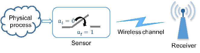
As shown in Fig. 1, we consider a status update system consisting of a sensor and a destination, where the sensor performs simple monitoring tasks, such as reading temperature, and the destination could be a monitor or an actuator. The status update system is assumed to be time-slotted. The sensor may produce a status update about the underlying time-varying process (a.k.a. generate-at-will) in each time slot and send it over an unreliable wireless channel to the destination. The sensor could also remain idle in one time slot. Let $a_{t}\in\{0,1\}$ be the action of the sensor in the $t$-th slot, where $a_{t}=1$ indicates that the sensor samples and transmits an update, and $a_{t}=0$, otherwise. Any update’s transmission time is assumed to be equal to one slot length. Moreover, the slot length is normalized to unity, without loss of generality. In general, each update would entail a cost $C_{u}$, including the sampling cost and the transmission cost, where the cost for sampling is assume to be negligible compared to that of transmission.

Assume that the underlying time-varying physical process is modeled by a $M$-state discrete time Markov chain $\{X_{t};t\in\mathbb{N}\}$ with $X_{t}\in\{1,2,...,M\}$, where $M\geq 2$. The period of each state is equal to the length of one slot, and the transition occurs at the beginning of each slot just before the sampling decision. We assume that all the state of the Markov chain have have uniform stationary distribution.

We assume that the fading of channels in each slot stays constant but varies independently over various slots. We also assume that an update is transmitted by the sensor at a fixed rate, and channel state information is only available at destination. As such, the transmission in each time slot may fail because of an outage and thus the loss of the packet could be described by a memoryless Bernoulli process. Specifically, let $h_{t}\in\{0,1\}$ denote whether the transmission succeeds or fails, where $h_{t}=1$ indicates that the transmission is successful, and $h_{t}=0$, otherwise. We define the success probability as $\Pr\{h_{t}=1\}=p_{s}$ and the failure probability as $\Pr\{h_{t}=0\}=p_{f}=1-p_{s}$. After the destination receives the update packet, a single-bit acknowledgement is fed back instantaneously without error. We assume that the failed update will be discarded, and if the sensor decides to transmit in the next slot, a new status update will be generated.¹¹ 1 The reason why we sample and transmit a new status update rather than retransmit a failed update lies in two aspects. On the one hand, according to the studies in [13], in the context of AoI, it is better not to retransmit an undecoded packet with the classical ARQ protocol, where failed transmissions are discarded at the destination and the receiver tries to decode each retransmission as a new message. This is because the probability of a successful transmission is the same for a retransmission and for the transmission of a new update. On the other hand, in this work we focus on the scenario that the sensor performs simple monitoring tasks, such as reading temperature, and hence, the cost for generating status packets is assumed to be negligible compared to that of transmission. Then, the energy costs for transmitting a new update and retransmitting a failed update are almost the same. Altogether, we choose to transmit a new update when the transmission failure occurs.

We assume that at the beginning of a slot a status update is generated and transmitted, and the destination will receive it at the end of the slot if the transmission succeeds. The AoI, commonly used to quantify the freshness of the information, is specified as the time elapsed since the generation of the latest status update received by the destination. Suppose that the latest status update successfully received by the destination was generated at the time instants $U(t)$, i.e., $U(t)=\max\{g_{i}\mid d_{i}\leq t\}$, where $g_{i}$ and $d_{i}$ represent the time instants when the update $i$ is generated and delivered, respectively. Then, the AoI at the beginning of slot t is given by

The proposed metric, AoCI, is different from the AoI in that the AoCI not only captures the time lag of the update received at the destination, but also includes variations in the information content of these updates. In particular, the AoCI only declines when the newly received update content differs from the previous one, and boosts otherwise. Let us denote by $n(t)=\max\{i|d_{i}\leq t\}$ the index of the latest update the destination receives at the end of slot $t$. We let $Y_{j}$ denote the information content of update $j$. It is worth noting that $Y_{j}$ is equal to the state of the physical process in the slot when update $j$ was generated, e.g., $Y_{n(t)}=X_{U(t)}$. Let us denote by $m(t)=\max\{j|Y_{j}\neq Y_{n(t)},d_{j}\leq d_{n(t)}\}$ the index of the most recently update which has different content from the latest update $n(t)$ got. Then, we can define the AoCI at the beginning of slot $t$ as

where $U^{\prime}(t)=\min\{g_{k}|d_{m(t)}<d_{k}\leq d_{n(t)}\}$ represents the generation time of the next successfully received update after $m(t)$. Noting that all the update packets that have been successfully received after $m(t)$ have the same content as the latest one received. We set the upper limits to the AoCI and the AoI, which are denoted by $\hat{\Delta}$ and $\hat{\delta}$, respectively.

In slot $t$ where a status update is received successfully, we denote by $D_{t}\in\{0,1\}$ an indicator for whether the content of the newly received update varies from that of the previously received update. If $D_{t}=1$, then the newly received update has different content. Otherwise, it has the same content. Particularly, the content change probability is defined as

where $p_{r}(\delta_{t})=\Pr(X_{U(t)}=X_{U(t)-\delta_{t}})$ is the return probability that the state of the physical process remains the same after $\delta_{t}$ steps. In the above equation, (a) holds due to the definition of $D_{t}$, and (b) holds because of the fact that $Y_{n(t)}=X_{U(t)}$ and $Y_{n(t)-1}=X_{U(t)-\delta_{t}}$.²² 2 Note that the time difference between two consecutive samples at the sensor is $\delta_{t}$. Therefore, the update $n(t)-1$ was generated at $U(t)-\delta_{t}$, and its content $Y_{n(t)-1}$ is the same as the state of the physical process at $U(t)-\delta_{t}$, i.e., $X_{U(t)-\delta_{t}}$. According to (2), if a new status update generated by the sensor is received successfully by the destination (i.e., $a_{t}=1,h_{t}=1$) and it contains different content from the update previously received (i.e., $D_{t}=1$), then the AoCI decreases to one; otherwise, the AoCI increases by one. Then, the dynamics of the AoCI is given by

For ease of exposition, we demonstrate how the AoCI and the AoI evolve over time in Fig. 2, where the dotted line represents the AoI and the solid line represents the AoCI.

The aim of this paper is to find an update policy $\pi=(a_{0},a_{1},\ldots)$ that minimizes the total average cost, which is defined as the weighted sum of the AoCI and the update cost. By defining $\Pi$ as a set of stationary and deterministic policies,³³ 3 A policy is said to be stationary and deterministic if it is time invariant and chooses an action with probability one. our problem is formulated as follows:

where $\omega$ is the weighting factor and the expectation is taken with respect to the distribution over trajectories induced by $\pi$ together with the transition probabilities.

The optimization problem in (5) can be cast into an infinite horizon average cost Markov decision process $(\mathcal{S},\mathcal{A},\Pr(\cdot|\cdot,\cdot),C(\cdot,\cdot))$, where each element is described as follows:

• •

  States: The state of the MDP at time slot $t$ is defined to be the tuple of the AoCI and the AoI, i.e., $\bm{s}_{t}\triangleq\left(\Delta_{t},\delta_{t}\right)$. Since both the AoCI and the AoI are bounded by their upper limits, the state space $\mathcal{S}$ is finite.

• •

  Actions: The action at time slot $t$ is $a_{t}$ and the action set is $\mathcal{A}=\{0,1\}$.

• •

  Transition Probability: Let $\Pr(\bm{s}_{t+1}|\bm{s}_{t},a_{t})$ denote the transition probability that state transits from $\bm{s}_{t}$ to $\bm{s}_{t+1}$ by taking action $a_{t}$ at slot $t$. Because the event of packet transmission and that of content change are independent, according to the AoCI evolution dynamics (4), the transition probability is represented as in (6) and $\Pr(\bm{s}_{t+1}|\bm{s}_{t},a_{t})=0$ otherwise.

• •

  Cost: We let $C(\bm{s}_{t},a_{t})=\Delta_{t}+\omega a_{t}C_{u}$ denote the instantaneous cost at state $\bm{s}_{t}$ given action $a_{t}$.

The above MDP is a finite-state finite-action average-cost MDP. According to [24, Theorem 8.4.5], there exists a deterministic stationary average optimal policy for the finite-state finite-action average-cost MDP if the cost function is bounded and the MDP is unichain, i.e., the Markov chain corresponding to every deterministic stationary policy consists of a single recurrent class plus a possibly empty set of transient states. Below, we examine these two conditions. First, the cost of the above MDP is bounded since the instantaneous cost is defined as the weighted sum of the AoCI and the energy consumption. Second, since the state $(\hat{\Delta},\hat{\delta})$ is reachable from all other states, the induced Markov chain has a single recurrent class. Hence, the MDP is unchain. Altogether, there exists a stationary and deterministic optimal policy. The optimal policy $\pi^{*}$ to minimize the total average cost can be obtained by solving the following Bellman equation [25]:

where $\theta$ is the optimal value to (5) for all initial state and $V(\bm{s})$ is the value function which is a mapping from $\bm{s}$ to real values. Moreover, for any $\bm{s}\in\mathcal{S}$, the optimal policy can be given by

We can seen from (8) that the optimal policy $\pi^{*}$ depends on the value function $V(\cdot)$. Unfortunately, there is usually no closed-form solution for $V(\cdot)$ [25]. Therefore, numerous numerical algorithms have been proposed in the literature, such as policy iteration and value iteration. Nonetheless, owing to the curse of dimensionality these approaches are typically computationally exhausting, and few insights can be leveraged for optimal policy. Hence, in the sequel, we study the structural properties of the optimal updating policy.

To analyze the structure of $\pi^{*}$, we introduce the state-action value function $Q(\bm{s},a)$, which is defined as

for all $\bm{s}\in\mathcal{S}$ and $a\in\mathcal{A}$. Note that $Q(\bm{s},a)$ is related to the RHS of the Bellman equation in (7). The optimal policy can also be expressed in terms of $Q(\bm{s},a)$, i.e.,

Before we present the main theorem, we first show the key properties of the value function $V(\Delta,\delta)$ in the following lemmas.

We first consider a special case where the return probability $p_{r}(\delta)$ is irrespective of $\delta$, i.e., $p_{r}(\delta_{1})=p_{r}(\delta_{2})\neq 0$ for any $\delta_{1}\neq\delta_{2}$. It is easy to see that the condition in Theorem 1 is satisfied in this special case and the optimal updating policy has a threshold structure with respect to the AoCI.

One example for this special case is that the state of the underlying physical process transits with equiprobability. The one-step state transition probability matrix for $M$-state discrete time Markov chain is given by

where $p_{c}=\frac{1}{M}$. Since the $\delta$-step state transition probability matrix $\Pr(X_{t+\delta}|X_{t})$ is the same with $\Pr(X_{t+1}|X_{t})$ for all $\delta$, we have $p_{r}(\delta)=1/M$.

In this case, we can simplify the MDP formulated in Section III.A. In particular, the state at slot $t$ is only the AoCI, i.e., $s_{t}=\Delta_{t}$, and the state transition probability in (6) can be simplified as

and $\Pr(s_{t+1}|s_{t},a_{t})=0$ otherwise.

Based on the simplified state and transition probability, we present the monotonicity property of $V(s)$ in the following lemma.

In this case, we consider that $p_{r}(1)=0$ and $p_{r}(\delta)\geq 0$ for $\delta>1$. It is also easy to see that the condition in Theorem 1 is satisfied in this special case and the optimal updating policy has a special structure with respect to the AoCI as given in Theorem 1. The optimal updating policy can also be obtained via Algorithm 1.

The example for this case is the physical process modeled by periodic Markov chain. For instance, the Markov model could be a $M$-state one-dimensional random walk with the state transition probability matrix given by

where $p_{c}\in(0,1)$ and $M$ is even. Every state of this Markov chain is periodic with period 2. Hence, the return probability $p_{r}(\delta)$ is $0$ when $\delta$ is odd, and is positive when $\delta$ is even.

In Figs. 5 and 6, we illustrate the analytical results of Theorem 1 when Markov model of the physical process is a one-dimensional random walk with 4-state and 6-state, respectively. The period of both Markov chain is 2. In both figures, the optimal updating policy is shown to have a special structure with respect to the AoCI for any $\delta$. In fact, the structure of the optimal policy unveils a tradeoff between the AoCI and the update cost. Particularly, if the AoCI is small, it is not efficient for the sensor to send the status update to the destination due to the update cost. It can also be seen that the optimal action $\pi^{*}=0$ does not appear in the whole state space of the AoCI if the AoI is high. This is due to the fact that the AoCI is always no less than the AoI and it is more efficient to generate a new status update due to the outdated information at the destination with the high AoI.

In Fig. 7, we compare the total average cost of the optimal policy and two baseline policies with respect to $p_{s}$. It can be observed in Fig. 7 (a) that the optimal policy outperforms the zero-wait policy. Moreover, as $p_{s}$ increases, there is a larger reduction in the total average cost. The reason can be explained with the aid of Fig. 7 (b). Although the zero-wait policy gains a smaller AoCI, it bears a constant update cost. In contrast, the optimal policy can trade off the AoCI for the update cost. Particular, in the optimal policy, the sensor remains idle until the AoCI is larger than a threshold, thereby inducing a large AoCI. However, the optimal policy has a smaller update cost than the zero-wait policy. We also observe that the sample-at-change policy outperforms the optimal policy at first. As $p_{s}$ increases, the optimal policy beats the sample-at-change policy, because the update cost of the optimal policy declines as $p_{s}$ increases. Hence, the optimal policy is more cost-efficient.

In Fig. 8, we compare the total average cost of the optimal policy and two baseline policies with respect to $M$, where $p_{c}$ is set to be $1/M$. We can see in Fig. 8 (a) that the optimal policy outperforms both baseline policies. Moreover, for both the optimal policy and the zero-wait policy, when $M$ grows, the total average cost decreases. As shown in Fig. 8 (b), the average AoCI of the optimal policy is larger than that of the zero-wait policy, whereas the average update cost of the optimal policy is smaller than that of the zero-wait policy. The average AoCI decreases with the increasing of $M$ because the received status update is more likely to have a new content with a large $M$. The average update cost is affected by $M$ and the optimal threshold simultaneously. The increase of the average update cost when $M=4$ is due to the decrease of the optimal threshold as shown in Fig. 4. When the optimal threshold is fixed, the average update cost decreases as $M$ increases. We also observe that the total average cost of the sample-at-change policy increases with $M$. This is because the return probability decreases with $M$ and the sample-at-change policy approaches the zero-wait policy as $M$ increases.

In Fig. 9, we compare the total average cost of the optimal policy and two baseline policies with respect to $p_{s}$. It can be observed that the optimal policy outperforms both two baseline policies. As $p_{s}$ increases, both the AoCI and the update cost of the optimal policy decline. This is because the AoCI can be reset with fewer transmission when $p_{s}$ is large. The AoCI of both baseline policy decreases with the increase of $p_{s}$. However, the update cost of the zero-wait policy remains constant and the update cost of the sample-at-change policy increases with $p_{s}$. In particular, the sample-at-change policy degenerates to zero-wait policy when $p_{s}=1$. As a result, the performance gain of the optimal policy is larger when $p_{s}$ is larger.

In Fig. 10, we compare the total average cost of the optimal policy and two baseline policies with respect to $\omega$. From Fig. 10 (a), we can observe that the total average cost of three policies increase with the weighting factor $\omega$. The three policies are coincident when $\omega=0$, which implies that the sensor under the optimal policy would sample and transmit in each time slot. As $\omega$ increases, the total average cost of the zero-wait policy and the sample-at-change policy grow linearly. This is because these two baseline policies cannot adapt to the weighting factor and its average AoCI and average update cost are constant, as shown in Fig. 10 (b). On the contrary, the optimal policy is able to adjust according to $\omega$. When $\omega$ grows larger, the AoCI is traded off to obtain a smaller update cost. Therefore, the optimal policy can strike a balance between the AoCI and the update cost.

We prove Lemma 1 through mathematical induction and the value iteration algorithm (VIA) [25]. We first briefly introduce VIA. For each state $\bm{s}$, let $V_{k}(\bm{s})$ be the value function at iteration $k$. In VIA, the value function can be updated as follows:

Under any initialization of the initial value $V_{0}(\bm{s})$, the sequence $\{V_{k}(\bm{s})\}$ converges to the value function in the Bellman equation (7) [25], i.e.,

Therefore, the monotonicity of $V(\bm{s})$ in $\mathcal{S}$ can be guaranteed by proving that for any $\bm{s}_{1},\bm{s}_{2}\in\mathcal{S}$, such that $\bm{s}_{1}\leq\bm{s}_{2}$,

According to (19), the monotonicity of $V(\bm{s})$ with respect to the AoCI can be guaranteed by proving that for any $\bm{s}_{1}=(\Delta_{1},\delta),\bm{s}_{2}=(\Delta_{2},\delta)\in\mathcal{S}$, such that $\Delta_{1}\leq\Delta_{2}$,

Then, we prove (21) via mathematical induction. Without loss of generality, we initialize $V_{0}(\bm{s})=0$ for all $\bm{s}\in\mathcal{S}$. Thus, (21) holds for $k=0$. Next, we assume that (21) holds up till $k>0$ and we examine whether it holds for $k+1$.

When $a=0$, we have $Q_{k}(\bm{s}_{1},0)=\Delta_{1}+\mathop{V_{k}(\bm{s}^{\prime}_{1})}$ and $Q_{k}(\bm{s}_{2},0)=\Delta_{2}+\mathop{V_{k}(\bm{s}^{\prime}_{2})}$, where $\bm{s}^{\prime}_{1}=(\Delta_{1}+1,\delta+1)$ and $\bm{s}^{\prime}_{2}=(\Delta_{2}+1,\delta+1)$. Since $\Delta_{1}+1\leq\Delta_{2}+1$ and $V_{k}(\bm{s}^{\prime}_{1})\leq V_{k}(\bm{s}^{\prime}_{2})$, we can easily see that $Q_{k}(\bm{s}_{1},0)\leq Q_{k}(\bm{s}_{2},0)$.

When $a=1$, we have

and

Since $V_{k}(\Delta_{1},\delta)\leq V_{k}(\Delta_{2},\delta)$ for any $\delta$, we can also verify that $Q_{k}(\bm{s}_{1},1)\leq Q_{k}(\bm{s}_{2},1)$.

Altogether, we can assert that $V_{k+1}(s_{1})\leq V_{k+1}(s_{2})$ for any $k$. By taking limits on both sides of (21) and by (19), we complete the proof of Lemma 1.

Let $\bm{s}_{1}=(\Delta_{1},\delta)$ and $\bm{s}_{2}=(\Delta_{2},\delta)$. Based on Lemma 1, we have

and

Since $V({\bf s})=\underset{a}{\min}Q({\bf s},a)$, we can prove $V(\bm{s}_{2})-V(\bm{s}_{1})\geq\Delta_{2}-\Delta_{1}$ in four cases as follows:

• •

  Case 1: If $V(\bm{s}_{1})=Q(\bm{s}_{1},0)$ and $V(\bm{s}_{2})=Q(\bm{s}_{2},0)$, then $V(\bm{s}_{2})-V(\bm{s}_{1})=Q(\bm{s}_{2},0)-Q(\bm{s}_{1},0)\geq\Delta_{2}-\Delta_{1}$.

• •

  Case 2: If $V(\bm{s}_{1})=Q(\bm{s}_{1},1)$ and $V(\bm{s}_{2})=Q(\bm{s}_{2},1)$, then $V(\bm{s}_{2})-V(\bm{s}_{1})=Q(\bm{s}_{2},1)-Q(\bm{s}_{1},1)\geq\Delta_{2}-\Delta_{1}$.

• •

  Case 3: If $V(\bm{s}_{1})=Q(\bm{s}_{1},0)\leq Q(\bm{s}_{1},1)$ and $V(\bm{s}_{2})=Q(\bm{s}_{2},1)$, then $V(\bm{s}_{2})-V(\bm{s}_{1})=Q(\bm{s}_{2},1)-Q(\bm{s}_{1},0)\geq Q(\bm{s}_{2},1)-Q(\bm{s}_{1},1)\geq\Delta_{2}-\Delta_{1}$.

• •

  Case 4: If $V(\bm{s}_{1})=Q(\bm{s}_{1},1)\leq Q(\bm{s}_{1},0)$ and $V(\bm{s}_{2})=Q(\bm{s}_{2},0)$, then $V(\bm{s}_{2})-V(\bm{s}_{1})=Q(\bm{s}_{2},0)-Q(\bm{s}_{1},1)\geq Q(\bm{s}_{2},0)-Q(\bm{s}_{1},0)\geq\Delta_{2}-\Delta_{1}$.

This completes the proof of Lemma 2.

Let $\bm{s}_{1}=(\Delta,\delta_{1})$ and $\bm{s}_{2}=(\Delta,\delta_{2})$. We use mathematical induction and the VIA to prove Lemma 3. Specifically, we need to prove that for any $\delta_{1}\leq\delta_{2}$

if $p_{r}(\delta_{1})-p_{r}(\delta_{2})\leq\frac{\delta_{2}-\delta_{1}}{\mathop{V_{k}(\Delta+1,1)}-V_{k}(1,1)}$ for any $k$.

Without loss of generality, we initialize $V_{0}(\bm{s})=0$ for all $\bm{s}\in\mathcal{S}$. Thus, (26) holds for $k=0$. Next, we assume that (26) holds up till $k>0$ and we examine whether it holds for $k+1$.

When $a=0$, we have

When $a=1$, we have

References

- [1] W. Lin, X. Wang, C. Xu, X. Sun, and X. Chen, “Average Age Of Changed Information In The Internet Of Things,” in Proc. IEEE WCNC, May 2020, pp. 1–6.
- [2] M. R. Palattella, M. Dohler, A. Grieco, G. Rizzo, J. Torsner, T. Engel, and L. Ladid, “Internet of Things in the 5G Era: Enablers, Architecture, and Business Models,” IEEE J. Sel. Areas Commun., vol. 34, no. 3, pp. 510–527, Mar. 2016.
- [3] P. Schulz, M. Matthe, H. Klessig, M. Simsek, G. Fettweis, J. Ansari, S. A. Ashraf, B. Almeroth, J. Voigt, I. Riedel, A. Puschmann, A. Mitschele-Thiel, M. Muller, T. Elste, and M. Windisch, “Latency Critical IoT Applications in 5G: Perspective on the Design of Radio Interface and Network Architecture,” IEEE Commun. Mag., vol. 55, no. 2, pp. 70–78, Feb. 2017.
- [4] M. A. Abd-Elmagid, N. Pappas, and H. S. Dhillon, “On the Role of Age-of-Information in Internet of Things,” IEEE Commun. Mag., vol. 57, no. 12, pp. 72–77, 2019.
- [5] S. Kaul, R. Yates, and M. Gruteser, “Real-time status: How often should one update?” in Proc. IEEE INFOCOM, Orlando, FL, USA, Mar. 2012, pp. 2731–2735.
- [6] S. K. Kaul, R. D. Yates, and M. Gruteser, “Status updates through queues,” in Proc. CISS, Mar. 2012, pp. 1–6.
- [7] A. Kosta, N. Pappas, A. Ephremides, and V. Angelakis, “Age of Information Performance of Multiaccess Strategies with Packet Management,” http://arxiv.org/abs/1812.09201, Dec. 2018.
- [8] C. Xu, H. H. Yang, X. Wang, and T. Q. S. Quek, “Optimizing Information Freshness in Computing-Enabled IoT Networks,” IEEE Internet Things J., vol. 7, no. 2, pp. 971–985, Feb. 2020.
- [9] Y.-P. Hsu, E. Modiano, and L. Duan, “Scheduling Algorithms for Minimizing Age of Information in Wireless Broadcast Networks with Random Arrivals,” IEEE Trans. Mob. Comput., vol. 19, no. 12, pp. 2903–2915, 2020.
- [10] Y. Sun, E. Uysal-Biyikoglu, R. D. Yates, C. E. Koksal, and N. B. Shroff, “Update or Wait: How to Keep Your Data Fresh,” IEEE Trans. Inf. Theory, vol. 63, no. 11, pp. 7492–7508, Nov. 2017.
- [11] A. M. Bedewy, Y. Sun, S. Kompella, and N. B. Shroff, “Age-optimal Sampling and Transmission Scheduling in Multi-Source Systems,” http://arxiv.org/abs/1812.09463, Dec. 2018.
- [12] J. Liu, P. Tong, X. Wang, B. Bai, and H. Dai, “UAV-Aided Data Collection for Information Freshness in Wireless Sensor Networks,” IEEE Trans. Wirel. Commun., pp. 1–1, 2020.
- [13] E. T. Ceran, D. Gündüz, and A. György, “Average Age of Information With Hybrid ARQ Under a Resource Constraint,” IEEE Trans. Wirel. Commun., vol. 18, no. 3, pp. 1900–1913, Mar. 2019.
- [14] H. Tang, J. Wang, L. Song, and J. Song, “Minimizing Age of Information With Power Constraints: Multi-User Opportunistic Scheduling in Multi-State Time-Varying Channels,” IEEE J. Sel. Areas Commun., vol. 38, no. 5, pp. 854–868, May 2020.
- [15] B. Zhou and W. Saad, “Joint Status Sampling and Updating for Minimizing Age of Information in the Internet of Things,” IEEE Trans. Commun., vol. 67, no. 11, pp. 7468–7482, Nov. 2019.
- [16] S. Leng and A. Yener, “Age of Information Minimization for an Energy Harvesting Cognitive Radio,” IEEE Trans. Cogn. Commun. Netw., vol. 5, no. 2, pp. 427–439, Jun. 2019.
- [17] M. A. Abd-Elmagid, H. S. Dhillon, and N. Pappas, “A Reinforcement Learning Framework for Optimizing Age of Information in RF-Powered Communication Systems,” IEEE Trans. Commun., vol. 68, no. 8, pp. 4747–4760, Aug. 2020.
- [18] ——, “AoI-Optimal Joint Sampling and Updating for Wireless Powered Communication Systems,” IEEE Trans. Veh. Technol., vol. 69, no. 11, pp. 14 110–14 115, Nov. 2020.
- [19] Y. Sun and B. Cyr, “Sampling for data freshness optimization: Non-linear age functions,” J. Commun. Netw., vol. 21, no. 3, pp. 204–219, Jun. 2019.
- [20] C. Kam, S. Kompella, G. D. Nguyen, J. E. Wieselthier, and A. Ephremides, “Towards an effective age of information: Remote estimation of a Markov source,” in IEEE INFOCOM WKSHPS, Honolulu, HI, USA, Apr. 2018, pp. 367–372.
- [21] J. Zhong, R. D. Yates, and E. Soljanin, “Two Freshness Metrics for Local Cache Refresh,” in Proc. IEEE ISIT, Vail, CO, Jun. 2018, pp. 1924–1928.
- [22] H. Tang, J. Wang, Z. Tang, and J. Song, “Scheduling to Minimize Age of Synchronization in Wireless Broadcast Networks With Random Updates,” IEEE Trans. Wirel. Commun., vol. 19, no. 6, pp. 4023–4037, Jun. 2020.
- [23] A. Maatouk, S. Kriouile, M. Assaad, and A. Ephremides, “The Age of Incorrect Information: A New Performance Metric for Status Updates,” IEEEACM Trans. Netw., vol. 28, no. 5, pp. 2215–2228, Oct. 2020.
- [24] M. L. Puterman, Markov Decision Processes: Discrete Stochastic Dynamic Programming, ser. Wiley Series in Probability and Statistics. Hoboken, NJ: Wiley-Interscience, 2005.
- [25] Dimitri P. Bertsekas, Dynamic Programming and Optimal Control-II, 3rd ed. Athena Scientific, 2007, vol. II.
- [26] M. L. Littman, T. L. Dean, and L. P. Kaelbling, “On the complexity of solving Markov decision problems,” in Proceedings of the Eleventh Conference on Uncertainty in Artificial Intelligence, ser. UAI’95. San Francisco, CA, USA: Morgan Kaufmann Publishers Inc., Aug. 1995, pp. 394–402.