Domain walls in the coupled Gross–Pitaevskii equations with the harmonic potential

Let $\varepsilon>0$ be a small parameter for the semi-classical (Thomas–Fermi) limit. We consider a real-valued solution $\Psi=(\psi_{1},\psi_{2})$ to the following coupled system of Gross–Pitaevskii equations with the harmonic potential and the cubic nonlinear terms:

where $\gamma>0$ is the coupling parameter. The Thomas-Fermi limit corresponds to the asymptotic regime with $\varepsilon\to 0$.

System (1.1) is the Euler–Lagrange equation for the following energy functional

for $\Psi=(\psi_{1},\psi_{2})$ defined in the energy space $\mathcal{E}:=H^{1}({\mathbb{R}};\mathbb{R}^{2})\cap L^{2,1}({\mathbb{R}};\mathbb{R}^{2})$, where $L^{2,1}({\mathbb{R}}):=\{f\in L^{2}({\mathbb{R}}):\;|x|f\in L^{2}({\mathbb{R}})\}$.

In order to introduce the steady states of the coupled system of Gross–Pitaevskii equations, let us first describe the ground state of the scalar Gross–Pitaevskii equation with the harmonic potential.

Let $\eta_{\varepsilon}\in H^{1}({\mathbb{R}};\mathbb{R})\cap L^{2,1}({\mathbb{R}};\mathbb{R})$ be the positive solution of the differential equation

The positive solution shown on Fig. 1 has been studied in the literature in many details [15, 21, 22]. The formal limit $\varepsilon\to 0$ corresponds to the so-called Thomas-Fermi cloud $\eta_{0}$ of the form

By Proposition 2.1 in [21], the positive solution $\eta_{\varepsilon}$ satisfies

and

moreover, $\eta_{\varepsilon}$ converges to $\eta_{0}$ in the sense that for every compact subset $K$ of $\{\left|{x}\right|<1\}$, there exists a constant $C_{K}>0$ such that

Refined asymptotic properties of $\eta_{\varepsilon}$ were further obtained in [15], where existence of $\eta_{\varepsilon}$ was obtained from the Hasting–McLeod solution of the Painlevé-II equation. By Theorem 1 in [15], there exists a constant $C>0$ such that

Equation (1.3) is the Euler–Lagrange equation for the following energy functional

By using the transformation

and making the change of variables $x\to z:=x/\varepsilon$, we obtain $G_{\varepsilon}(\Psi)=F_{\varepsilon}(\eta_{\varepsilon})+\varepsilon J_{\varepsilon}(\Phi)$, where

for $\Phi=(\phi_{1},\phi_{2})$ defined in $H^{1}_{\rm loc}({\mathbb{R}};{\mathbb{R}}^{2})$ for which $J_{\varepsilon}(\Phi)<\infty$.

Since $\lim\limits_{\varepsilon\to 0}\eta_{\varepsilon}(\varepsilon z)=\eta_{0}(0)=1$ for every $z\in{\mathbb{R}}$, the formal limit of (1.11) is the energy functional studied in [5]:

The Euler–Lagrange equations for $J_{0}(\Phi)$ is the coupled system of homogeneous Gross–Pitaevskii equations without the harmonic potential:

A symmetric pair of domain wall solutions exists for $\gamma>1$ as minimizers of $J_{0}$ by Theorem 1.1 in [5] (see [39] for earlier mathematical results and [31] for the first fundamental result in physics literature). One particular domain wall solution $\Phi=(\phi_{1},\phi_{2})$ to the system (1.13) satisfies the following boundary conditions:

whereas the other domain wall can be obtained by the transformation $\phi_{1}\leftrightarrow\phi_{2}$.

Theorems 2.1, 2.4, and 3.1 in [5] state that $(\phi_{1},\phi_{2})$ for the domain wall solution with the boundary conditions (1.14) satisfies the following properties:

• (a)

  $\phi_{2}(z)=\phi_{1}(-z)$ for all $z\in\mathbb{R}$;

• (b)

  $\phi_{1}^{2}(z)+\phi_{2}^{2}(z)\leq 1$ for all $z\in\mathbb{R}$;

• (c)

  $\phi_{1}^{\prime}(z)>0$ and $\phi_{2}^{\prime}(z)<0$ for all $z\in\mathbb{R}$.

Uniqueness of domain walls with properties (a)–(c) was shown in [4] and more generally in [13]. Orbital stability of domain walls in the coupled system of Gross–Pitaevskii equations was established in a weighted Hilbert space in [9].

We introduce three steady state solutions to system (1.1) that will be studied in this work.

1. (S1)

   For every $\gamma>0$, there exist uncoupled states

   $$\psi_{1}(x)=\eta_{\varepsilon}(x),\quad\psi_{2}(x)=0,\quad\mbox{\rm and}\quad\psi_{1}(x)=0,\quad\psi_{2}(x)=\eta_{\varepsilon}(x).$$

   (1.15)

2. (S2)

   For every $\gamma>0$, there exists the symmetric state

   $$\psi_{1}(x)=\psi_{2}(x)=(1+\gamma)^{-1/2}\eta_{\varepsilon}(x).$$

   (1.16)

3. (S3)

   We say that the solution is the domain wall state if $\psi_{1}(x)=\psi_{2}(-x)$ for all $x\in\mathbb{R}$ but $\psi_{1}(x)\not\equiv\psi_{2}(x)$.

Both the symmetric state (S2) and the domain wall state (S3) are defined in the energy space with the symmetry given by

One domain wall state (S3) with the property $\psi_{1}(x)>\psi_{2}(x)>0$ for $x>0$ is shown on Fig. 2. Another domain wall state can be obtained by the transformation $\psi_{1}\leftrightarrow\psi_{2}$. Existence, variational characterization, and bifurcations of the domain wall state (S3) are the main subjects of this work.

Our first theorem establishes a rigorous connection between problems (1.1) and (1.13). Recall the product form (1.10) which reduces the minimization problem for $G_{\varepsilon}$ to one for $J_{\varepsilon}$. A consequence of Lemma 2.1 below is that $\Psi\in\mathcal{E}$ minimizes $G_{\varepsilon}$ if and only if $\Phi\in H^{1}_{\rm loc}({\mathbb{R}};{\mathbb{R}}^{2})$ minimizes $J_{\varepsilon}$. Furthermore, we prove that $J_{\varepsilon}$ converges to $J_{0}$ in the sense of $\Gamma$-convergence [11].

In view of the decomposition $G_{\varepsilon}(\Psi)=F_{\varepsilon}(\eta_{\varepsilon})+\varepsilon J_{\varepsilon}(\Phi)$, Theorem 1 establishes a relation between minimizers of $G_{\varepsilon}$ for small $\varepsilon>0$ and those of the limiting functional $J_{0}$. This relation was one of the motivations for studying domain walls in [5, 9] as minimizers of $J_{0}$ for $\gamma>1$ with prescribed limits at infinity.

The functional $J_{0}$ also possesses critical points $(1,0)$, $(0,1)$, and $(1+\gamma)^{-1/2}(1,1)$, which correspond to the steady states (S1) and (S2) in the limit $\varepsilon\to 0$. The question of their variational characterization for $\gamma>1$ was left open in [5]. The case $0<\gamma<1$ was not considered in [5]. The following two theorems clarify the variational characterization of the three steady states (S1), (S2), and (S3) as critical points of the energy $G_{\varepsilon}$.

The bifurcation curve $\gamma=\gamma_{0}(\varepsilon)$ is shown on Fig. 3 on the $(\varepsilon,\gamma)$ plane. Domain wall states (S3) are global minimizers of the energy $G_{\varepsilon}$ in $\mathcal{E}_{s}$ above the bifurcation curve. The blue dotted curve shows the straight line $\gamma=1$. The magenta dotted curve shows the approximation of the bifurcation curve explained below.

It follows from the exponential decay of the domain wall states of the homogeneous system (1.13) to the boundary conditions (1.14) that the domain wall states without the harmonic potential only exist for $\gamma>1$, where they are minimizers of the energy $J_{0}$ [5]. It is surprising that we are not able to derive a similar result for the domain wall states (S3) in the case of the harmonic potential. By uniqueness of positive solutions of the coupled system (1.1) in Theorem 2, the domain wall do not exist for $\gamma\in(0,1)$, but we do not have a similar non-existence result for $\gamma\in[1,\gamma_{0}(\varepsilon)]$. By Theorem 3, the domain wall states exist and are minimizers of the energy $G_{\varepsilon}$ if $\gamma\in(\gamma_{0}(\varepsilon),\infty)$.

In order to understand more properties in the construction of the domain wall states (S3), we introduce the Dirichlet condition $\psi_{1}(0)=\psi_{2}(0)=\alpha$ and define the energy space on the half-line:

The following theorem states that if $\alpha>0$ is fixed and the non-symmetric critical points of $G_{\varepsilon}$ exist in $D_{\alpha}$, they are minimizers of $G_{\varepsilon}$ in $D_{\alpha}$. Unfortunately, this result does not eliminate the domain wall states in $\mathcal{E}_{s}$ for $\gamma\in[1,\gamma_{0}(\varepsilon)]$ since such states could be saddle points of $G_{\varepsilon}$ with respect to varying $\alpha$.

Next, we study bifurcations of the steady states. The exceptional case $\gamma=1$ in Theorem 2 is special since the nonlinear system (1.1) with $\gamma=1$ has an additional rotational symmetry which results in the existence of the following one-parameter family of solutions:

where $\theta\in[0,\frac{\pi}{2}]$ is required for positivity of solutions. The family of solutions (1.21) recovers (S1) if $\theta=0$ or $\theta=\frac{\pi}{2}$ and (S2) if $\theta=\frac{\pi}{4}$. The following theorem suggests that the domain wall state (S3) does not bifurcate from the one-parameter family (1.21), in agreement with Theorem 3.

When $\gamma=1$ and $\varepsilon=0$ (black dot on Fig. 3), the energy $J_{0}$ ceases to impose segregation of the two components and hence, a natural question is to identify the valid asymptotic behavior of the domain walls in the limit $(\varepsilon,\gamma)\to(0,1)$. We do so by using the rescaling

where

Since $\varepsilon=\mu\sqrt{\gamma-1}$ and $\mu>0$ is fixed, the formal limit of (1.22) as $\gamma\to 1^{+}$ is

where ${\mathcal{I}_{\mu}}:=(-\frac{1}{\mu},\frac{1}{\mu})$.

Minimizers of $I_{\mu,1}$ in (1.23) are shown on Fig. 4 by dashed line together with the numerical approximation of the domain wall state shown by the solid line for $\varepsilon=0.1$ and $\gamma=1.2$. Both solutions are shown versus the original coordinate $x$. The agreement implies the relevance of the asymptotic approximation found from $I_{\mu,1}$.

A rigorous connection between the two energy functionals $I_{\mu,\gamma}$ and $I_{\mu,1}$ given by (1.22) and (1.23) is established in Lemma 4.1 below, where $\Gamma$ convergence of $I_{\mu,\gamma}$ to $I_{\mu,1}$ is shown for fixed $\mu>0$.

The following theorem states the existence of a special $\mu_{0}\in(0,\infty)$ separating the symmetric state (S2) and the domain wall state (S3) as minimizers of $I_{\mu,1}$ in the energy space with symmetry $\mathcal{E}_{s}$. The curve $\varepsilon=\mu_{0}\sqrt{\gamma-1}$ is shown on Fig. 3 by the magenta dotted line, illustrating a good approximation for the bifurcation curve $\gamma=\gamma_{0}(\varepsilon)$.

If we wish to set $\mu=0$ in $I_{\mu,1}$, we obtain the limiting energy for the energy functional $J_{0}$ in the sense of $\Gamma$-convergence:

The domain wall state (S3) can be found explicitly as a minimizer of $I_{0,1}$ since the symmetric state (S2) corresponding to $\theta_{1}=\theta_{2}=\frac{1}{\sqrt{2}}$ is a saddle point by Theorem 6. Using the representation $(\theta_{1},\theta_{2})=(\sin(u),\cos(u))$ on the circle $\theta_{1}^{2}+\theta_{2}^{2}=1$ yields $I_{0,1}(\Theta)$ rewritten as $I_{0,1}(u)$ in the form:

with the corresponding Euler–Lagrange equation given by

The domain wall state in $\mathcal{E}_{s}$ corresponds to the restriction $\theta_{1}(y)=\theta_{2}(-y)$ for $y\in\mathbb{R}$. In particular, $\theta_{1}(0)=\theta_{2}(0)=\frac{1}{\sqrt{2}}$ which yields the condition $u(0)=\frac{\pi}{4}$. The boundary conditions $\theta_{1}(y)\to 0$ as $y\to-\infty$ and $\theta_{1}(y)\to 1$ as $y\to+\infty$ yields the conditions $u(y)\to 0$ as $y\to-\infty$ and $u(y)\to\frac{\pi}{2}$ as $y\to+\infty$. The unique solution of the differential equation (1.25) satisfying these requirements is found in the form:

This solution is the asymptotic approximation as $\gamma\to 1$ of the domain walls of the coupled system (1.13) without the harmonic potential. This explicit approximation was not obtained in [5].

By Theorem 2, the domain wall states (S3) are not global minimizers of $G_{\varepsilon}$ in $\mathcal{E}$ in their range of existence. In [5], domain walls were obtained variationally as heteroclinics to specific limits at infinity. Another approach to constructing domain walls is to consider a problem in the energy space with a spatial symmetry denoted by $\mathcal{E}_{s}$ and defined in (1.17). By Theorem 3, the domain wall states (S3) are global minimizers of $G_{\varepsilon}$ in $\mathcal{E}_{s}$ for $\gamma\in(\gamma_{0}(\varepsilon),\infty)$.

The effective numerical method for computation of domain walls is developed by working in the energy space $\mathcal{D}_{\alpha}$ on the half-line defined in (1.20) subject to the Dirichlet condition $\psi_{1}(0)=\psi_{2}(0)=\alpha$ with $\alpha>0$. The symmetric state in $\mathcal{D}_{\alpha}$ corresponds to the reduction $\psi_{1}(x)=\psi_{2}(x)$ for $x>0$. In addition, there may exist two non-symmetric states in $\mathcal{D}_{\alpha}$: one satisfies $\psi_{1}(x)>\psi_{2}(x)>0$ for $x>0$ and the other one is obtained by the transformation $\psi_{1}\leftrightarrow\psi_{2}$. By Theorem 4, if the non-symmetric states exist, they are global minimizers of the energy $G_{\varepsilon}$ in $\mathcal{D}_{\alpha}$.

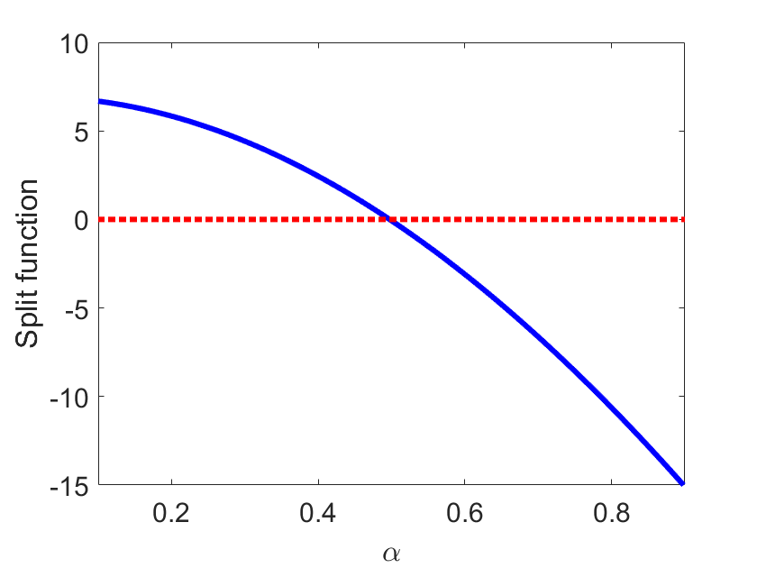
Non-symmetric minimizers of $G_{\varepsilon}$ in $\mathcal{D}_{\alpha}$ depend on $\alpha$ and recover the domain wall states (S3) on the half-line if the split function $S_{\varepsilon}(\alpha)$ vanishes, where

and the derivatives are well-defined because minimizers of $G_{\varepsilon}$ in $\mathcal{D}_{\alpha}$ are smooth on $\mathbb{R}_{+}$. Another criterion to identify the domain wall state (S3) as the global minimizers of $G_{\varepsilon}$ in $\mathcal{E}_{s}$ is to plot the energy level $G_{\varepsilon}(\Psi_{\alpha})$ versus $\alpha$, where $\Psi_{\alpha}$ is the non-symmetric minimizer of $G_{\varepsilon}$ in $\mathcal{D}_{\alpha}$, and to find the values of $\alpha$ for which $G_{\varepsilon}(\Psi_{\alpha})$ is minimal.

We have implemented both ways to find the domain wall states (S3) numerically. Non-symmetric minimizers of $G_{\varepsilon}$ in $\mathcal{D}_{\alpha}$ were approximated numerically with a second-order central-difference relaxation method. Fig. 5 shows how $S_{\varepsilon}(\alpha)$ and $G_{\varepsilon}(\Psi_{\alpha})$ depend on $\alpha$ for $\varepsilon=0.1$ and $\gamma=3$. Zero of $S_{\varepsilon}$ corresponds to the minimum of $G_{\varepsilon}(\Psi_{\alpha})$ and appears at $\alpha_{0}\approx 0.5$. The corresponding domain wall state extended from $\mathcal{D}_{\alpha_{0}}$ by the symmetry condition in space $\mathcal{E}_{s}$ is shown on Fig. 2.

Performing numerical approximations in the range of values of $\gamma$, we can obtain a family of domain wall states by using this method. Fig. 6 shows the dependence of the optimal value of $\alpha=\psi_{1}(0)=\psi_{2}(0)$ found from the root of $S_{\varepsilon}$ versus $\gamma$ by solid line. Iterations of the numerical method do not converge near $\gamma=1$ since the domain wall states are minimizers of $G_{\varepsilon}$ in $\mathcal{E}_{s}$ only for $\gamma\in(\gamma_{0}(\varepsilon),\infty)$ by Theorem 3 with $\gamma_{0}(\varepsilon)>1$ for $\varepsilon>0$. The dashed line shows the linear interpolation between the limiting value $\alpha_{0}=\frac{1}{\sqrt{2}}$ found from the limiting energy (1.23) shown by the blue dot and the last numerical data point at $\gamma=1.2$.

Fig. 4 (solid line) shows the domain wall state at $\varepsilon=0.1$ and $\gamma=1.2$. In order to find the minimizer of $I_{\mu,1}$ in (1.23), we write $(\theta_{1},\theta_{2})=(\sin(u),\cos(u))$ and solve the corresponding Euler–Lagrange equation

The Euler–Lagrange equation (1.27) is solved numerically subject to the conditions $u(0)=\frac{\pi}{4}$ and $u^{\prime}(y)>0$ for $y\in(-\mu^{-1},\mu^{-1})$. The solution is concatenated with the constant solution $u(y)=u(\mu^{-1})$ for $y\in(\mu^{-1},\infty)$ and $u(y)=u(-\mu^{-1})$ for $y\in(-\infty,-\mu^{-1})$. The second-order central-difference relaxation method is used to obtain the numerical approximation of $u(y)$, which is then plotted versus the original coordinate $x$.

Fig. 1 is obtained by using the same relaxation method for the stationary equation (1.3) on $\mathbb{R}_{+}$ subject to the conditions $\eta_{\varepsilon}^{\prime}(0)=0$ and $\eta_{\varepsilon}(x)\to 0$ as $x\to\infty$.

The bifurcation curve $\gamma=\gamma_{0}(\varepsilon)$ on Fig. 3 is obtained by numerical approximation of eigenvalues of the Hessian operator at the symmetric state (S2) in the proof of Theorem 3. Eigenvalues of the Dirichlet problem for the Schrödinger operator

are shown on Fig. 7. They are monotonically decreasing in $\gamma$ and the crossing point of the first (smallest) eigenvalue of $L_{\gamma}$ gives the bifurcation curve $\gamma=\gamma_{0}(\varepsilon)$. The same second-order central-difference method is applied to approximate derivatives of the Schrödinger operator $L_{\gamma}$ on $\mathbb{R}_{+}$ subject to the Dirichlet condition at $x=0$. The spatial domain is truncated on $[0,3]$ similar to Fig. 1.

The magenta dotted curve on Fig. 3 is obtained from the first (smallest) eigenvalue $\nu_{0}:=\mu_{0}^{-2}$ of the boundary-value problem

arising in the proof of Theorem 6. With the transformation $x=\tanh(\xi)$ which maps $[0,1]$ to $\mathbb{R}_{+}$, the boundary-value problem (1.29) is rewritten in the form

The spatial domain of this boundary-value problem is truncated on $[0,10]$ resulting in the lowest eigenvalue at $\nu_{0}\approx 7.29$. The asymptotic approximation on Fig. 3 corresponds to $\gamma=1+\nu_{0}\varepsilon^{2}$.

The remainder of this paper contains proofs of the main theorems.

Section 2 gives the proof of the splitting formula $G_{\varepsilon}(\Psi)=F_{\varepsilon}(\eta_{\varepsilon})+\varepsilon J_{\varepsilon}(\Phi)$ (Lemma 2.1) and the proof of Theorem 1 about $\Gamma$ convergence of $J_{\varepsilon}$ to $J_{0}$.

Section 3 gives proofs of Theorems 2 and 3 and identify the parameter ranges for which the uncoupled, symmetric, and domain wall states are the global minimizers of the energy $G_{\varepsilon}$ in the energy space $\mathcal{E}$ and in the energy space with symmetry $\mathcal{E}_{s}$. The bifurcation at $\gamma=\gamma_{0}(\varepsilon)$ and the Schrödinger operator $L_{\gamma}$ in (1.28) arise in the proof of Theorem 3. Existence of minimizers of $G_{\varepsilon}$ in $\mathcal{E}$ is given by Lemma 3.1. Lemma 3.2 describes properties of the domain wall states (S3) as minimizers of $G_{\varepsilon}$ in $\mathcal{E}_{s}$. Lemma 3.3 gives uniqueness of the symmetric state (S2) as the positive solution of the coupled system (1.1) if $\gamma\in(0,1)$. Finally, we prove Theorem 4 about the non-symmetric minimizers of $G_{\varepsilon}$ in $\mathcal{D}_{\alpha}$ with fixed $\alpha>0$.

Section 4 investigates bifurcations from the one-parameter family of solutions (1.21) at $\gamma=1$ establishing the proof of Theorem 5. Lemma 4.1 gives $\Gamma$-convergence of the energy functional $I_{\mu,\gamma}$ to $I_{\mu,1}$ as $\gamma\to 1^{+}$. The bifurcation $\mu=\mu_{0}$ and the boundary-value problem (1.29) arise in the proof of Theorem 6 from analysis of $I_{\mu,1}$ at the symmetric state. Lemma 4.2 gives uniqueness of the symmetric state if $\mu\in[\mu_{0},\infty)$. Lemma 4.3 reports computations of the normal form for bifurcation of domain wall states and shows that the domain wall states bifurcate to $\mu<\mu_{0}$, where they are characterized as minimizers of $I_{\mu,1}$ if $\mu\in(0,\mu_{0})$.

As we have pointed out previously, the proof that the domain wall states (S3) only exist if $\gamma>\gamma_{0}(\varepsilon)$, where they are characterized as minimizers of $G_{\varepsilon}$, is open for further studies.

Acknowledgements. The work of A.C. was partially supported by a grant from the Simons foundation # 426318. V. S. acknowledges support by Leverhulme grant RPG-2018-438. D. P. is supported by the NSERC Discovery grant.

References

• [1] A. Aftalion and R. Rodiac. “One dimensional phase transition problem modeling striped spin orbit coupled Bose-Einstein condensates”, J. Differ. Equ. 269 (2020) 38–81.
• [2] A. Aftalion, J. Royo-Letelier. “A minimal interface problem arising from a two component Bose-Einstein condensate via Γ\Gamma-convergence”, Calc. Var. 52 (2015) 165–197.
• [3] A. Aftalion and E. Sandier. “Vortex patterns and sheets in segregated two component Bose-Einstein condensates”, Calc. Var. 59 (2020) 19 (38 pages).
• [4] A. Aftalion and C. Sourdis. “Interface layer of a two-component Bose–Einstein condensate”, Commun. Contemp. Math 19 (2017) 1650052 (46 pages).
• [5] S. Alama. L. Bronsard, A. Contreras, and D. Pelinovsky, “Domain walls in the coupled Gross-Pitaevskii equations” Arch. Rat. Mech. Appl. 215 (2015) 579–615.
• [6] P. Ao and S. T. Chui. “Binary Bose-Einstein condensate mixtures in weakly and strongly segregated phases”, Phys. Rev. A 58 (1998) 4836–4840.
• [7] R. A. Barankov. “Boundary of two mixed Bose-Einstein condensates”, Phys. Rev. A 66 (2002) 013612.
• [8] R. N. Bisset, R. M. Wilson, and C. Ticknor, “Scaling of fluctuations in a trapped binary condensate”, Phys. Rev. A 91 (2015), 053613 (6 pages).
• [9] A. Contreras, D.E. Pelinovsky, and M. Plum, “Orbital stability of domain walls in coupled Gross–Pitaevskii systems”, SIAM J. Math. Anal. 50 (2018) 810–833.
• [10] M.G. Crandall, and P.H. Rabinowitz, “Bifurcation from simple eigenvalues”, J. Funct. Anal. 8 (1971) 321–340.
• [11] G. Dal Maso, An Introduction to Γ\Gamma-Convergence, Progress in Nonlinear Differential Equations and Their Applications, Birkhäuser, Boston, 1993
• [12] N. Dror, B.A. Malomed, J. Zeng. “Domain walls and vortices in linearly coupled systems”, Phys. Rev. E 84 (2011) 046602.
• [13] A. Farina, B. Sciunzi, and N. Soave, “Monotonicity and rigidity of solutions to some elliptic systems with uniform limits”, Commun. Contemp. Math. 22 (2020) 1950044 (24 pages).
• [14] C. Gallo and D.E. Pelinovsky, “Eigenvalues of a nonlinear ground state in the Thomas-Fermi approximation”, J. Math. Anal. Appl. 355 (2009) 495–5261.
• [15] C. Gallo and D. Pelinovsky, “On the Thomas-Fermi ground state in a harmonic potential”, Asymptotic Analysis 73 (2011) 53–96.
• [16] M. Goldman and J. Royo-Letelier. “Sharp interface limit for two components Bose-Einstein condensates”, ESAIM: COCV 21 (2015) 603-624.
• [17] M. Goldman and B. Merlet. “Phase Segregation for Binary Mixtures of Bose-Einstein Condensates”, SIAM J. Math. Anal. 49 (2017) 1947-1981.
• [18] Q. Han, FH. Lin, Elliptic Partial Differential Equations, (1997), Courant Lecture Notes.
• [19] W. Han, S. Zhang, J. Jin and W. M. Liu. “Half-vortex sheets and domain-wall trains of rotating two-component Bose-Einstein condensates in spin-dependent optical lattices”, Phys. Rev. A 85 (2012) 043626.
• [20] I. Ianni and S. Le Coz. “Multi-speed solitary wave solutions for nonlinear Schrödinger systems”, J. London Math. Soc. 89 (2014) 623–639.
• [21] R. Ignat, V. Millot, “The critical velocity for vortex existence in a two-dimensional rotating Bose-Einstein condensate”, J. Funct. Anal. 233 (2006) 260–306.
• [22] R. Ignat, V. Millot, “Energy expansion and vortex location for a two-dimensional rotating Bose-Einstein condensate”, Rev. Math. Phys. 18 (2006) 119–162.
• [23] R. Ignat, L. Nguyen, V. Slastikov, A. Zarnescu, “Stability of the melting hedgehog in the Landau–de Gennes theory of nematic liquid crystals”, Archive for Rational Mechanics and Analysis, 215 (2015) 633–673.
• [24] R. Ignat, L. Nguyen, V. Slastikov, A. Zarnescu, On the uniqueness of minimisers of Ginzburg-Landau functionals, Annales Scientifiques de l’École Normale Supérieure. Quatrième Série, 53 (2020) 589–613.
• [25] K. Kasamatsu, H. Takeuchi, M. Tsubota and M. Nitta. Wall-vortex composite solitons in two-component Bose-Einstein condensates. Phys. Rev. A 88 (2013) 013620.
• [26] D. K. Maity, K. Mukherjee, S. I. Mistakidis, S. Das, P. G. Kevrekidis, S. Majumder, and P. Schmelcher, “Parametrically excited star-shaped patterns at the interface of binary Bose-Einstein condensates”, Phys. Rev. A 102 (2020), 033320 (13 pages)
• [27] L. Lassoued, P. Mironescu, “Ginzburg-Landau type energy with discontinuous constraint”, J. Anal. Math. 77 (1999) 1–26.
• [28] K. Law, P. G. Kevrekidis and L. S. Tuckerman. “Stable Vortex–Bright-Soliton Structures in Two-Component Bose-Einstein Condensates”, Phys. Rev. Lett. 105 (2010) 160405.
• [29] B. A. Malomed, “Past and present trends in the development of the pattern-formation theory: domain walls and quasicrystals”, Physics (2021), in print.
• [30] M. I. Merhasin, B. A. Malomed, and R. Driben, “Transition to miscibility in a binary Bose-Einstein condensate induced by linear coupling”, J. Physics B 38 (2005), 877–892.
• [31] V. M. Mineev, “The theory of the solution of two near-ideal Bose gases”, Sov. Phys. JETP 40 (1974), 132–136.
• [32] R. Navarro, R. Carretero–Gonzalez, and P.G. Kevrekidis, “Phase separation and dynamics of two-component Bose–Einstein condensates”, Phys. Rev. A 80 (2009) 023613 (14 pages).
• [33] N. V. Nguyen and Z. Wang. “Existence and stability of two-parameter family of solitary waves for a 2-coupled nonlinear Schrödinger system”, Discr. Cont. Dynam. Syst. 36 (2016) 1005–1021.
• [34] S. Pal, J.K. Bhattacharjee. “Dynamics of binary Bose–Einstein condensate via Ehrenfest like equations: appearance of almost shape invariant states”, Eur. Phys. J. D 71 (2017) 291.
• [35] J. Sabbatini, W. H. Zurek and M. J. Davis. “Phase separation and pattern formation in a binary Bose-Einstein condensate”, Phys. Rev. Lett. 107 (2011) 230402.
• [36] H. Takeuch, K. Kasamatsu, M. Nitta and M. Tsubota.“Vortex formations from domain wall annihilations in two-component Bose-Einstein condensates”, J. Low Temp. Phys. 162 (2011) 243–249.
• [37] G. Teschl, Ordinary Differential Equations and Dynamical Systems, Graduate Studies in Mathematics 140 (AMS, Providence RI, 2012).
• [38] M. Trippenbach, K. Goral, K. Rzazewski, B.A. Malomed, Y.B. Band. “Structure of binary Bose-Einstein condensates”, J. Phys. B: At. Mol. Opt. Phys. 33 (2000) 4017–4031.
• [39] G. Van den Berg and R. Van der Vorst, “A domain-wall between single-mode and bimodal states”, Diff. Integr. Eqs 13 (2000) 369–400.